Article

The Validation of a New GSTA Case in a Dynamic Coastal Environment Using Morphodynamic Modelling and Bathymetric Monitoring

1
Career Training & Planning Consultancy Ltd., Waterville, County Kerry 066 9474650, Ireland
2
MaREI, University College Cork, Ringaskiddy, Co.Cork T12 YN60, Ireland
*
Author to whom correspondence should be addressed.
J. Mar. Sci. Eng. 2016, 4(1), 27; https://doi.org/10.3390/jmse4010027
Submission received: 6 July 2015 / Revised: 26 February 2016 / Accepted: 2 March 2016 / Published: 17 March 2016
(This article belongs to the Special Issue Sediment Transport Modeling)

Abstract

:
Several methods of monitoring sediment transport exist and have varying degrees of success depending on the study sites characteristics. Grain Size Trend Analysis (GSTA) is an experimental method based on identifying transport trends from the variation of sediment grain characteristics within a defined study area. The parameters examined when performing GSTA are mean grain size, sorting coefficient and skewness, the most common cases found in field studies being; finer, better sorted and negatively skewed (FB−) or coarser, better sorted and positively skewed (CB+), as most transport trends follow one or the other trend. However, on Rossbeigh beach, Co. Kerry, Ireland, a coarser poorer and more negatively skewed (CP−) trend case gave the most realistic plot of sediment transport trend when compared with sediment transport calculation, bathymetry surveys, hydrodynamic monitoring and morphological modelling.

1. Introduction

Tracking sediment transport in the coastal zone has traditionally proven a difficult task due to the dynamic action of waves and tidal currents combined with large volumes of entrained sediment. Issues with equipment reliability and survivability have usually prevented comprehensive investigation, particularly in the surf zone. The need for data in this area is often critical to erosion and beach evolution studies, as most of the initial movement occurs in this zone. This was the case when undertaking a morphodynamic study of the breached barrier dune system in Dingle Bay, Co. Kerry, Ireland.
The barrier dunes protect Castlemaine Harbour, which is a brackish low-lying area of approximately 5300 Ha. Protection of the harbour is vital as it is both commercially and environmentally significant. It is a designated Special Area of Conservation (SAC) and wildfowl reserve as well as being a valuable clam, mussel, and salmon fishery. The beaches, which are both blue flag status, are an important tourist resource for the local economy.
The dune system had been in a state of dynamic equilibrium with shorelines eroding and prograding seasonally; however, a breach in the Rossbeigh dunes occurred in the winter of 2008 and has since widened to over 900 m. The impact this breaching has on the surrounding environment is multifaceted and potentially of significant economic impact. The loss of amenity and habitats is already occurring with the removal of protected dune; the change in sediment transport patterns is increasing sedimentation in the back barrier area and affecting aquaculture.
It is the reported [1] increase in flooding since the breaching event, however, that is potentially the greatest impact of the erosion in Rossbeigh. Approximately 100 homes and businesses are located on the low-lying (ground level, <10 m OD Malin) coastline directly behind the barrier beach. Anecdotal evidence [2] suggests that recent storm surge flooding corresponds to the emergence of the breach in the barrier beach. If present erosion trends continue, it is feared that flood risk in the back barrier will increase, thus increasing the potential economic loss.
A comprehensive examination of the entire coastal cell of Inner Dingle Bay was undertaken required before the extreme erosion occurring on Rossbeigh and consequently the morphodynamics of the barrier beach system could be understood. This included:
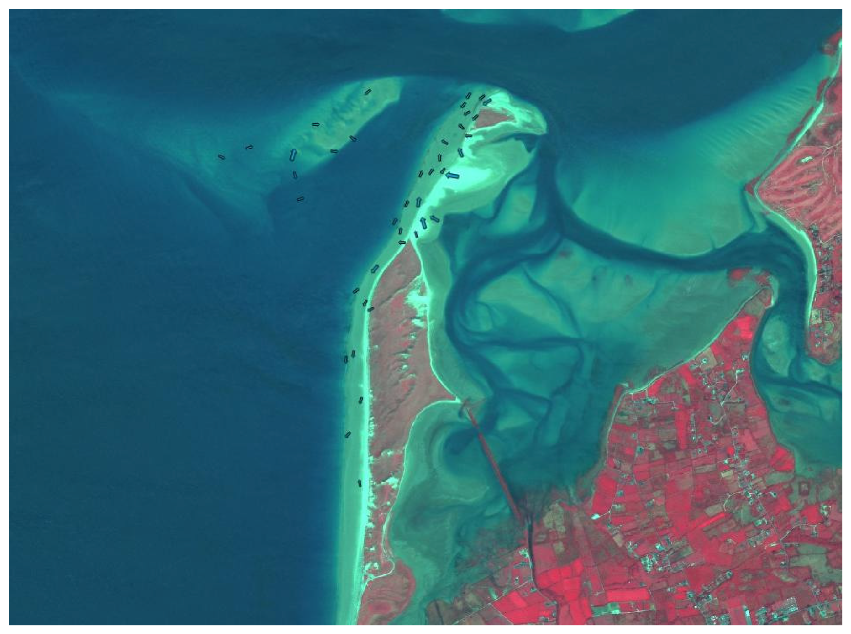
  • Gaining a deeper understanding of shoreline changes on Rossbeigh and Inch by examining alternative data sources including satellite imagery.
  • Undertaking regular topographic surveys to document the evolution of the breach area and Rossbeigh.
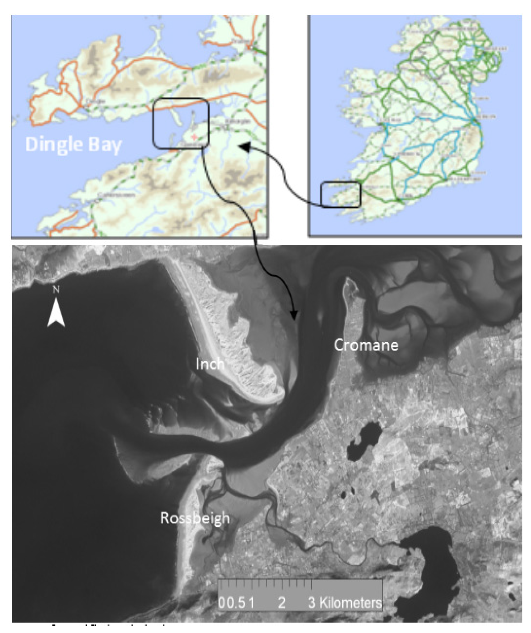
  • Characterising the wave climate and tidal current regime of Dingle Bay.
  • Conducting seasonal bathymetry surveys to identify where sediment is being transported to.
  • Investigate the applicability of novel and experimental methods on Inner Dingle Bay’s Barriers such as Grain Size Trend Analysis, Surface Wave Radar Monitoring and Sediment Dye Testing
Considering the other forms of analysis undertaken as part of the overall morphology study, results from GSTA on this site could be critically analysed and validated. Such case studies are in short supply. The main aims of undertaking GSTA on Rossbeigh were:
(1)
Establishing tangible sediment pathways to provide another insight into the morphology of Rossbeigh.
(2)
Provide a case study into the accuracy and applicability of the GSTA method in inlet-ebb tidal bar scenario.

2. Background

The basic theory behind grain size trend analysis (GSTA) is inferring sediment transport pathways from variations in sediment grain size characteristics sampled within the study area. The assumption is that the difference in grain size characteristics from one location to the next is due to the action of sediment transport in that direction.
Deriving sediment transport pathway trends by analysing sediment grain characteristics was initially investigated by Krumbein et al. [3]. They looked at the geographic variation of mean grain size of sediment samples and related it to a sediment transport pathways. This was improved upon by McLaren [4] who added skewness and sorting. These parameters are statistically derived from the grain size distribution curve of a sediment sample. Sorting is a function of the second moment and skewness a function of the third moment.
McLaren [4] suggested that although 8 cases are possible the trend analysis should only consider 2 cases, those being; finer, better sorted and negatively skewed (FB−) or coarser, better sorted and positively skewed (CB+), as most transport trends follow one or the other trend. Gao and Collins [5] suggested that all 8 cases could be analysed:
  • Finer, Better Sorted, Positively Skewed (FB+)
  • Finer, Poorer Sorted, Negatively Skewed (FP−)
  • Finer, Better Sorted, Negatively Skewed (FB−)
  • Finer, Poorer Sorted, Positively Skewed (FP+)
  • Coarser, Better Sorted, Positively Skewed (CB+)
  • Coarser, Poorer Sorted, Negatively Skewed (CP−)
  • Coarser, Better Sorted, Negatively Skewed (CB−)
  • Coarser, Poorer Sorted, Positively Skewed (CP+)
Gao and Collins [5] proposed method a two dimensional vectorial method expanding on the point to point 1-dimensional method of McLaren [4]. This method includes the filtering of noise by specifying a characteristic distance, Dcr. The points within this distance are used in the analysis of each point. Trend vectors are summed to produce a single vector then this is averaged to form a residual pattern. If patterns are similar then a pathway is defined.
LeRoux [6] argued against the filtering step and developed a method using trend analysis from the 4 closest neighbours. Since then, studies have used both methods with the Gao and Collins [5] method proving the more popular. The majority of trends on beaches have coincided with the original cases specified by McLaren [4] (FB− and CB+). These trends are usually supported by other monitoring activities in the coastal zone such as dye testing, bed form surveying and morphological modelling.
Poulos et al. [7] utilised the Gao and Collins [5] method to examining the effect of a dredged pit had on the sediment transport regime on the Kwinte Bank, southern North Sea. Sediment samples were taken pre and post dredging, and sediment trend analysis conducted. The results show a by-passing effect caused by the dredging.
However, other cases have also been identified such as FB+, by Poizot & Mear [8], in Cadiz Spain. This work goes further and suggests that two cases can occur on the same beach. A conceptual model was developed based on this theory proposing that FB+ dominates in the upper foreshore and FB− case is the dominant trend in the lower foreshore.
Poizot and Mear [9], have recently developed a GIS based GSTA tool called Gis Sed trend. This tool incorporates all of the various GSTA methodologies and the 8 different case tests previously mentioned. It allows the user to input data and vary parameters such as Dcr. There is also a facility to statistically test each result and display the trend vectors in a GIS format.

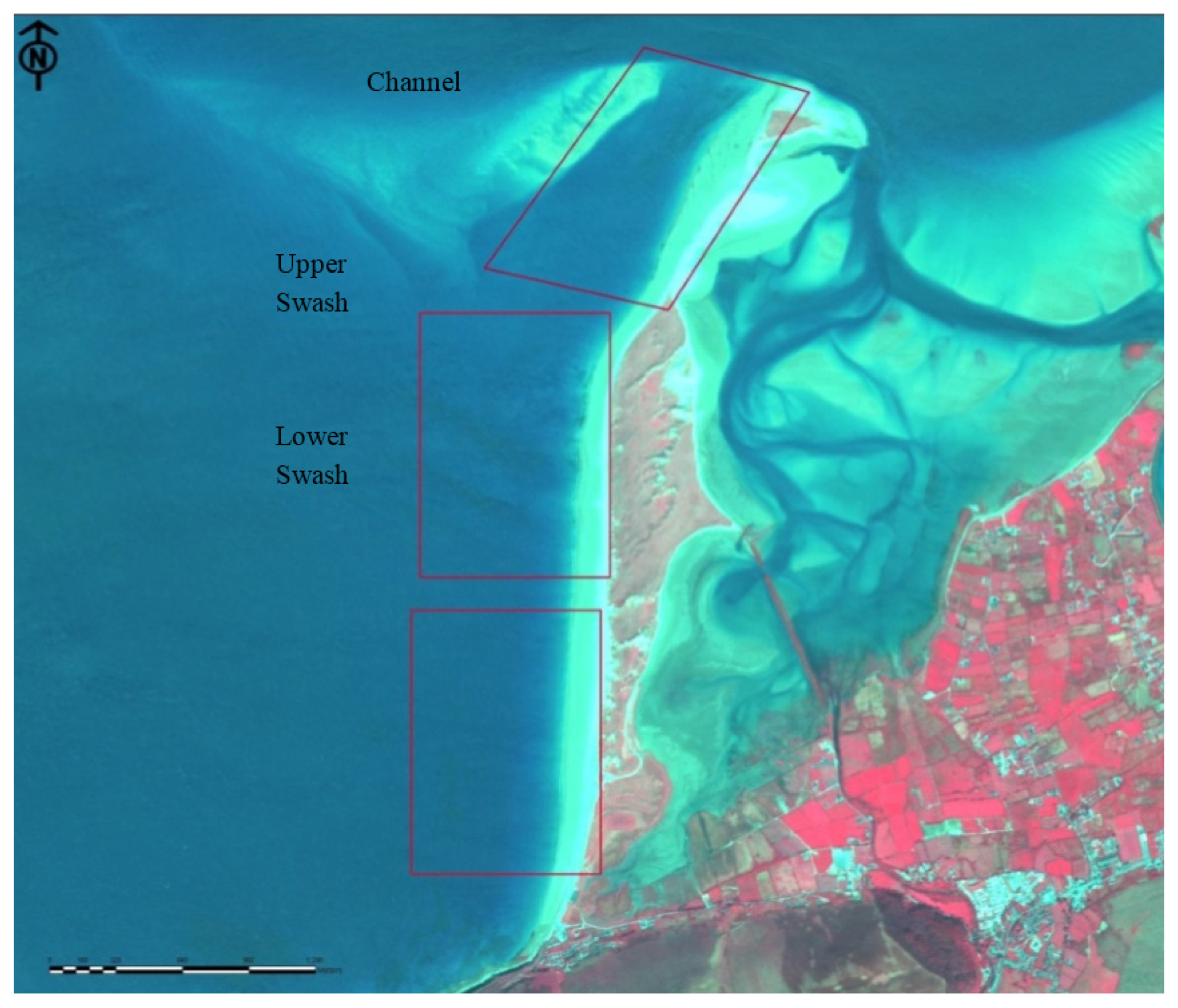
3. Environmental Setting

Dingle Bay, County Kerry, Ireland contains three barriers, Figure 1. The two outer barriers, Inch and Rossbeigh, extend across the bay divided by a tidal inlet. The low-lying barrier, Cromane, is located further inshore in the estuarine Castlemaine Harbour. The mean spring tidal range is approximately 3.2 m. The mean significant wave height (Hs) is 2.8 m and an average wave period (Tz) is 7 s based on 50 years of storm data analysis [10]. Dingle Bay incident wave directionality is narrow banded, as a result the inner bay can be classed as a self-contained coastal cell i.e., sediment transport is conserved within the bay [11]. The tidal inlet that separates Inch and Rossbeigh acts as an important sediment transport driver with tidal currents reaching over 1.0 m·s−1 at peak flood. It has been classified as mixed wave/tide dominated to tide dominated.

4. Experimental Setup

The study site was subject to a GSTA analysis to ascertain the suitability of such methods in calculating sediment transport pathways. The intertidal locations are suitable for such analysis given the sediment transport activity inherent in regular water level variation. Sixty samples were taken altogether, 18 on the ebb tidal bar and 42 along Rossbeigh beach. The sampling locations can be seen in Figure 2.
The sampling took place in April 2013 with wave conditions of between 0.25–0.50 m (Hs) in the previous week and a tidal range of 3.2 m. To ascertain correct sampling methodology, in particular the correct sample depth, consideration had to be given to the prevailing hydrodynamics that control sediment transport. In the present paper, disturbance depth is determined using the Saini et al.’s [12] formula which take into account wave conditions prior sampling:
Zm = 0.22 Hb
where
  • Zm = Depth of Disturbance
  • Hb = Breaking wave height
Defining a time period for the recent wave activity, in turn defines the time period related to the represented sediment pathway analysis. It is important to differentiate between recent and older sediment sorting patterns as confusion between the two is easily achieved through incorrect sample depth.
In the highly dynamic climate of Dingle Bay dye testing results, showed sample depths of 0.10 m were removed even in mild wave conditions on the drift aligned zone. This is more related to tidal current driven sediment transport which was not factored into established depth of disturbance formulae, such as Saini et al.’s [12] and others. The samples taken for GSTA were at 0.11 m deep.

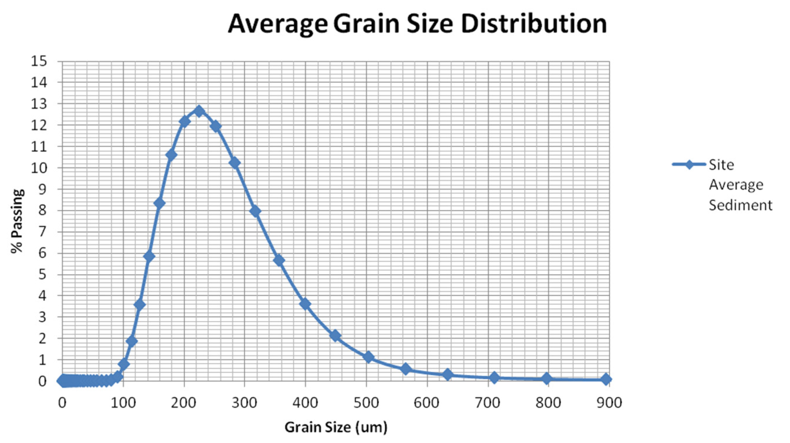
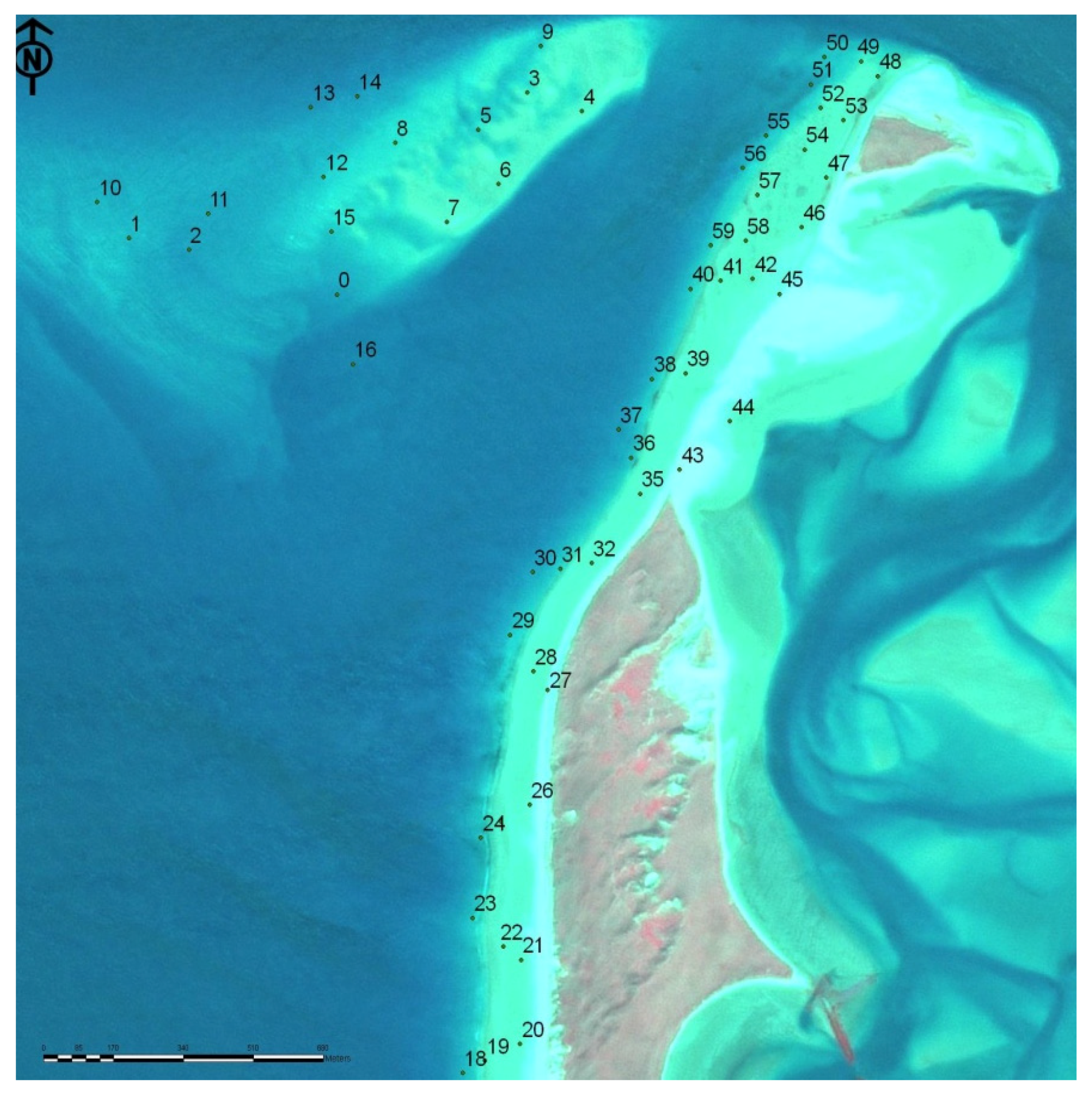
4.1. Sediment Sieving Analysis

Sediment samples were left to dry for one week. The samples were checked for shell and other erroneous elements before being processed for sieving. The sieving was undertaken by a Malvern Mastersizer Laser Diffractomer. The Malvern uses laser diffraction to measure the size of particles. A laser beam is passed through a sample and the intensity of light scattered was measured. This was then analysed to calculate the size of the particles that created the scattering pattern.
Five sub samples from each sample location were placed in the Laser diffractometer and an average sediment distribution for each location was calculated. Statistical analysis on the sample distributions was then undertaken. This involves calculating the three parameters necessary for GSTA; mean grain size, sorting and, skewness. A specific program called Gradistat, developed by Blott and Pye [13] was utilised to calculate the statistics for each sample location. The results of this are shown in Table 1.
The sediment statistics summarised by region are presented in Table 2. All three locations have similar averages except for the ebb tidal bar skewness. It is apparent that the swash aligned and the drift aligned zone share similar sorting statistics. The average granulometric curve is presented in Figure 3.

4.2. Numerical Model Set up

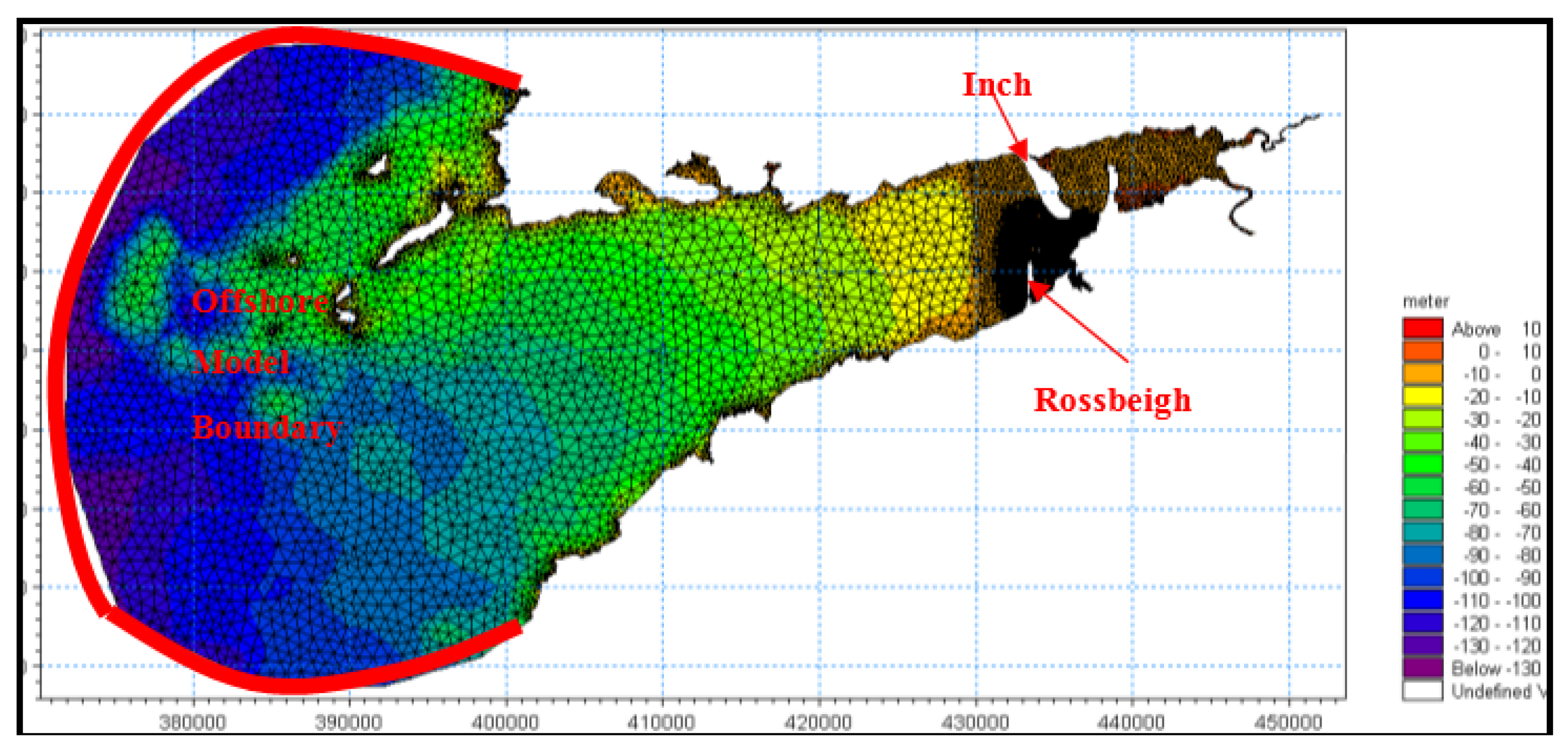
4.2.1. Model Domain and Boundary Conditions

A numerical model of Dingle Bay was created to simulate Wave, Tidal, Wind, Sediment transport and morphology within the study area. The model was developed to predict sediment transport trends on the barrier beaches.
The numerical model used was DHI Mike 21 [14] modelling software package consists of separate modules that compute wave forcings (SW), hydrodynamics (HD), sediment transport and morphology (ST) combined into one coupled model. The bathymetry of the model domain is represented on an unstructured mesh of quadrilateral and triangular shaped cells. The various model outputs are calculated at nodes in the centre of these cells.
The SW module calculates wave forcings based on the wave action conservation Formula (2) and solves the wave energy transfer function from initial boundary condition across the mesh using a finite volume method at the cell centers. Wind swell can also be incorporated in this module. This method is similar to the one used for the Delft 3D wave module SWAN (SWAN User Manual). Detailed information on the driving equations can be found in the manual [14]:
N t + V . ( v N ) = S σ
where N(x,σ,θ,t) = action density
  • t = time
  • x = (x, y) Cartesian co = ordinates
  • v = (cx, cy, cσ, cθ) the propagation velocity of a wave group in four dimensional space
  • S = the source term for energy balance equation
  • V = is the four dimensional operator in the x, σ,θ-space
The HD module calculates hydrodynamic forcings (tidal elevation and currents) utilising Navier stokes equations and applying a finite volume method similar to the SW module to solve the boundary condition of a tidal signal across the mesh. The coupling of these modules on the same mesh enables the simulation of current and wave interactions on the sediment transport and ultimately the morphology.
The sediment transport and morphology module (ST) applies the wave and hydrodynamic forcings generated at each node to drive sediment transport formulae [15]. The ST module requires several key inputs such as sediment particle size and morphological update frequency. The ST Module updates the bathymetry based on the sediment transport calculations in the model domain and effectively feeds back into the HD and SW modules during a simulation. To reduce computation time and increase model time scale a morphological speed up factor can be applied.
The Van Rijn Formula (3) predicts along shore transport rates including tidal current forcing, beach slope and grain size characteristics. The formula contains several coefficients empirically derived during beach studies and flume tests. This formula was chosen over others due to its relative success in describing sediment transport on Rossbeigh in O’Shea & Murphy [16].
Q t = K 0 K s w e l l K g r a i n K s l o p e ( H b ) 2.5 V e f f , L
where:
  • K0 = 42
  • Kswell = swell correction factor for swell waves <2 m, Kswell = Tswell/Tref
  • Kgrain = particle size correction factor
  • Kslope = bed slope correction factor
  • Veff.L = effective longshore velocity for tidal velocity component and wave induced velocity component.
The model domain, Figure 4, covered Dingle Bay extending from Castlemaine Harbour in the east to the open ocean beyond the mouth of Dingle Bay in the west. The model domain was represented on an unstructured mesh. The mesh cell density was varied, based on the complexity of the bathymetry, with density increasing moving from the open ocean in the west to Castlemaine Harbour beyond Rossbeigh in the east. The Dingle Bay model domain had three distinct levels of mesh density, an outer bay mesh, an intermediate density mesh in the middle of the bay and a high density mesh covering the area around the tidal inlet channel and Rossbeigh.
The wave and tidal input data were applied at the offshore model boundary. This model boundary encompassed the entrance to Dingle Bay in an arc shape. It was designed to ensure every possible wave direction incident in Dingle Bay could be simulated. A time series of water level elevation was applied at this boundary to simulate the tidal forcings in the bay. Likewise a time series of offshore wave data was applied at the offshore boundary to generate wave forcings incident in the bay.
A land boundary of the domain was also required to be defined. This process involved several iterations due to instabilities in the model at locations of sharp change in bathymetry/topography. Areas of the coastline on the northern shore of Dingle Bay were particularly susceptible to convergence errors. Reducing the severity of change in the land boundary and increasing the mesh density at these locations enabled the formulation of a stable model domain.

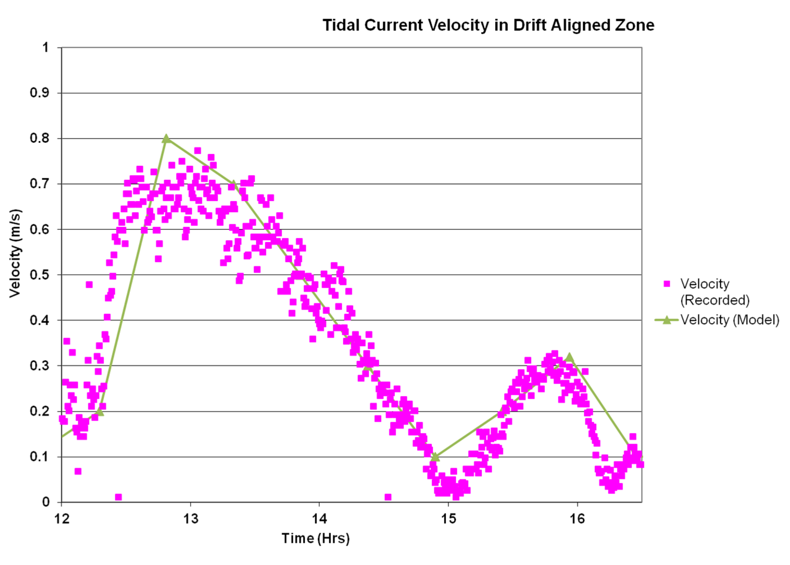
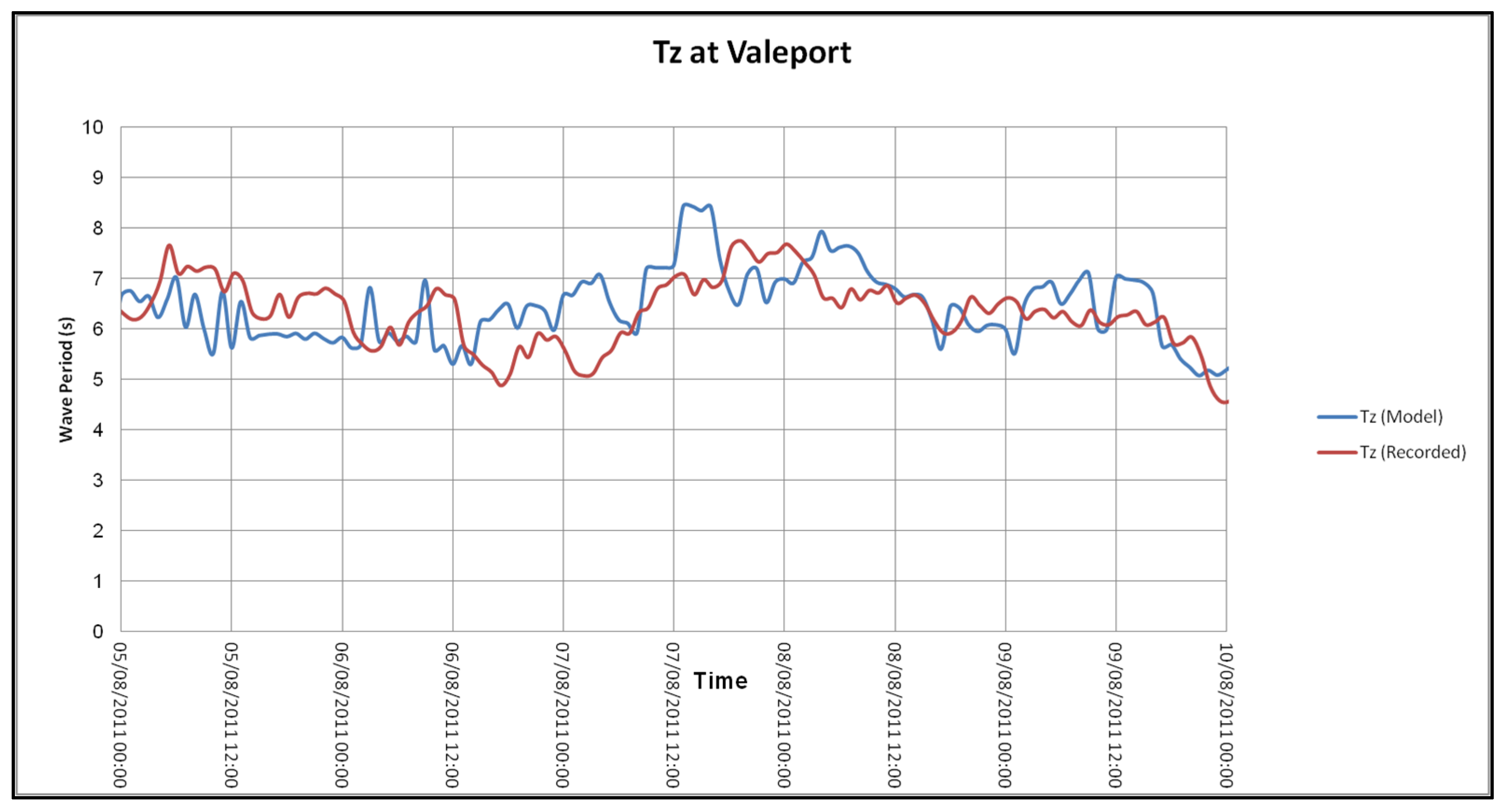
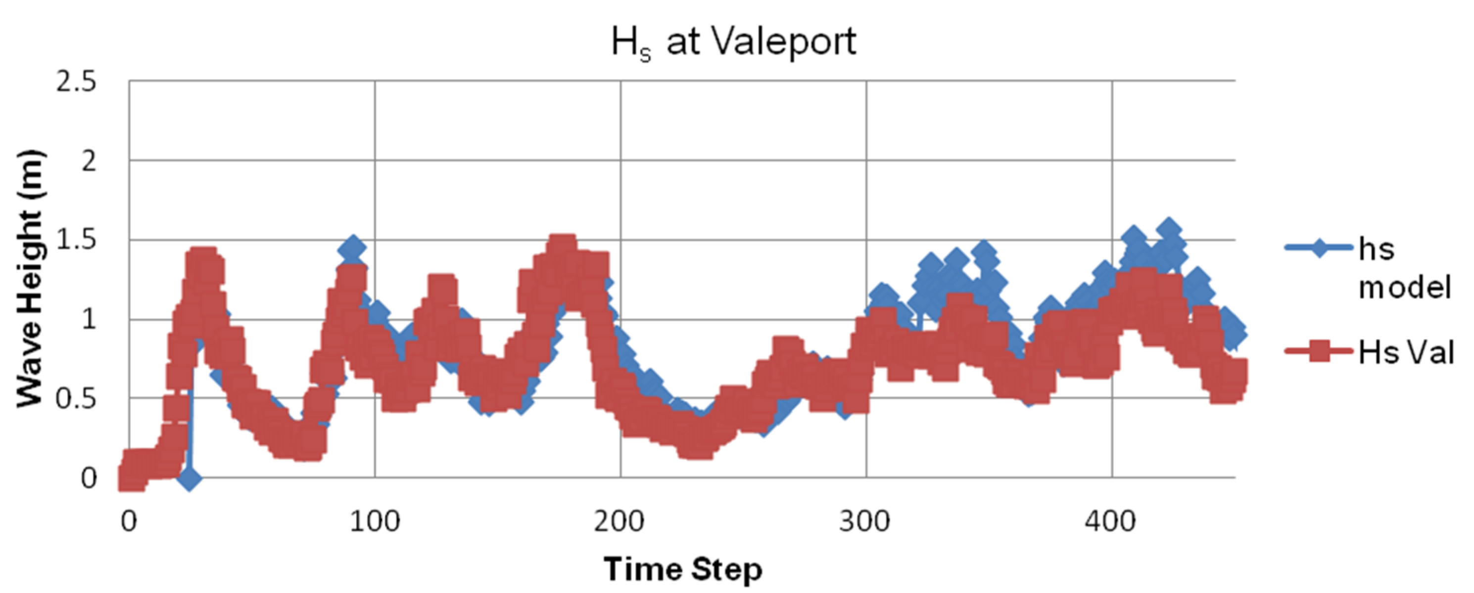
4.2.2. Model Validation

Validation of hydrodynamics and wave modules was necessary before morphodynamic modelling of Dingle Bay can be undertaken. The coupled HD and SW models were run with several parameters changed including bed roughness and diffraction coefficients and wave spreading before model results reproduced recorded data records. The following table, Table 3, details the final values of the critical model parameters.
The water surface elevation was validated against the recorded levels from a deployed gauge. The modelled tidal current velocity on the drift aligned zone of Rossbeigh beach, Figure 5 was compared with recorded current velocity measured during a field monitoring campaign as described [16].
The recorded peak flood velocity of 0.8 m·s−1 correlated well with the simulated velocities. The recorded secondary peak ebb velocity 0.3 m·s−1 in the diurnal tidal cycle also agreed with the simulated results.
The wave height and wave period was validated against a month of recorded data collected in 2011. The Wave data was recorded by a bottom mounted pressure sensor called a Valeport. The modelled wave period Tz shows good agreement with the period recorded at the wave gauge (Valeport) location, Figure 6. The recorded wave period displays less variability than the modelled period and has slightly larger peaks and greater minimum values.
The significant wave height, Hs also showed good correlation as can be seen in Figure 7.

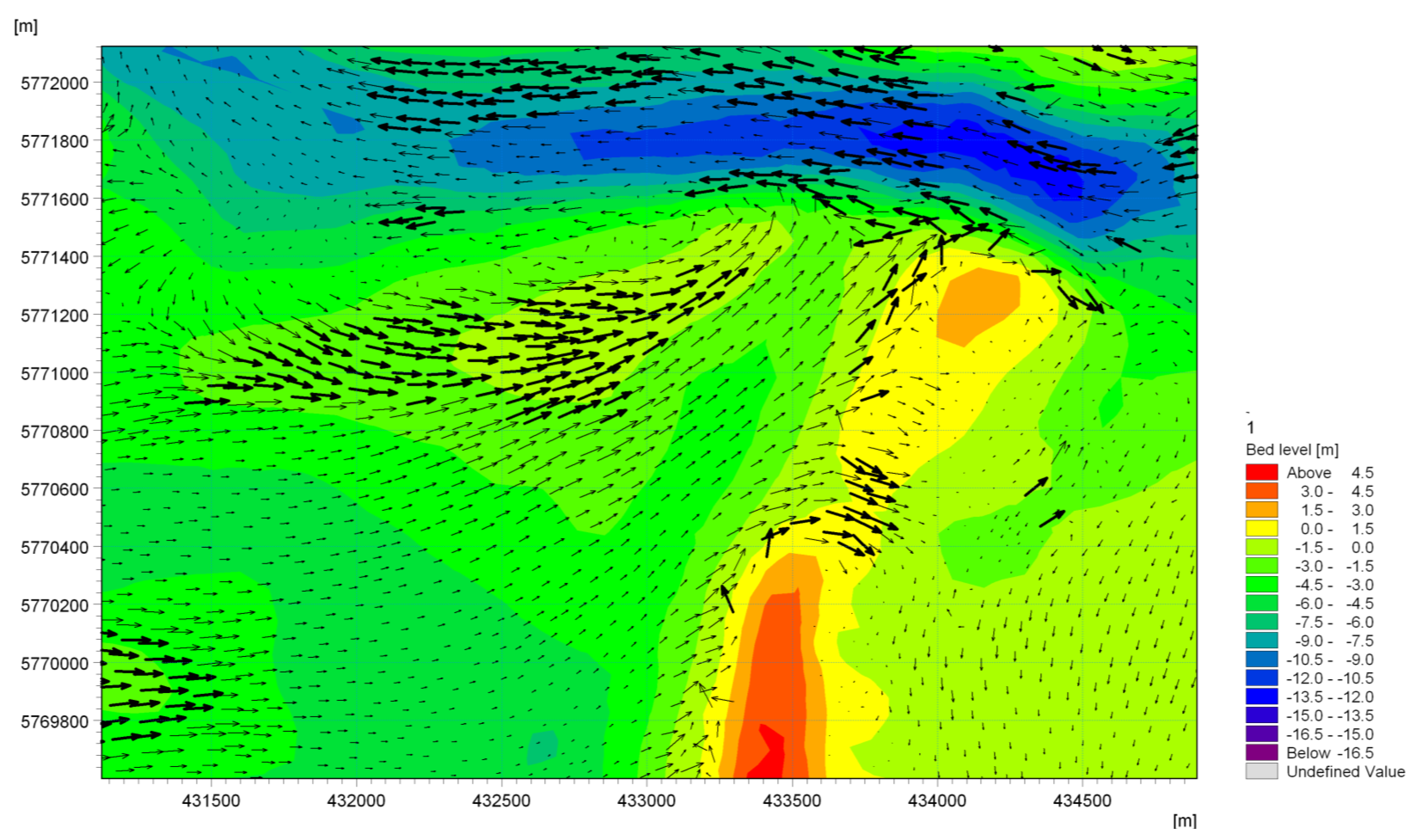
4.2.3. Sediment Transport and Morphology

To determine the accuracy of sediment transport and sediment transport modelling, a simulation of 6 months equivalent duration was run. The bed level volume changes were compared with the results of volume changes in bathymetric surveys over a 6 month period, from March 2013 to September 2013. The wave data time series of 1 month duration was used in the model. This data was representative of a mild climate and detailed previously [16].
In order to reduce computational runtime a morphological scale factor was applied to account for the acceleration of bed-level changes during updates at each hydrodynamic timestep. A morphological acceleration factor (Morfac) of 6 is applied to the model, simulating morphological changes that occurred over approximately 6 months utilising only 1 month of wave data.
The channel location, Figure 8, was selected to validate the sediment transport behavior as it had the highest density of recorded data points in the domain. Table 4 details the amount of sediment removed from the channel by using cut and fill volumes extracted from digital elevation models of the start and end bathymetry. The volume results from the model are similar to the surveyed volume changes. The cut volumes were within 15% of the survey while the fill volumes were within 5% of each other. The model over estimates the erosion rate but underestimates the fill rates slightly.

5. Results and Discussion

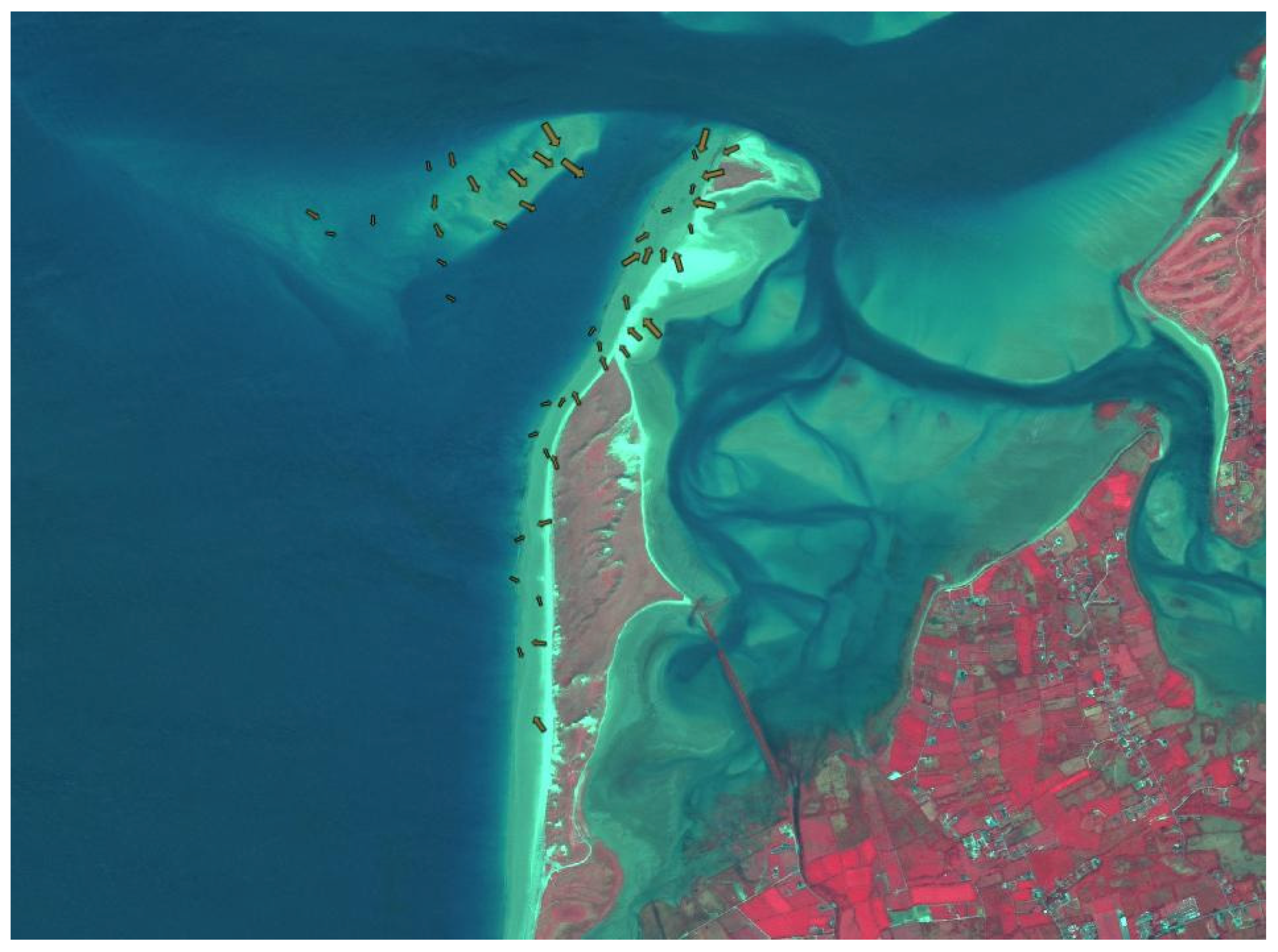
5.1. Grain Size Trend Analysis Results

Establishing a characteristic distance (Dcr) is the first step in GSTA. The Dcr calculated for the Rossbeigh site was 1050 m, this was achieved iteratively. Firstly an arbitrary distance, the average distance between points was chosen, this was then varied incrementally to establish the characteristic distance that gave the most suitable vector plots to the site. There are 8 different cases for GSTA, these relate to the various permutations of the three parameters, mean grain size, sorting and skewness. All eight permutations were tested using the GiSedTrend tool. It was evident that after initial visual analysis of the 8 cases only 4 resembled coastal sediment transport behaviour, CB+, FP−, CP− and FB+.
The analysis was initially split over two datasets, the beach of Rossbeigh and the ebb tidal bar. However, no difference in correlation of trends discussed below on the beach were observed. The results below discuss the analysis of a combined data set of Ebb tidal bar and Rossbeigh beach.
The Coarser Poorer and more negatively skewed (CP−) trend case gave the most realistic plot of sediment transport trend when compared with sediment transport calculation, bathymetry surveys, hydrodynamic monitoring and morphological modelling.
The results of this case are shown in Figure 9 along with 3 other test cases, CB+, FP− and FB+. The CB+, Figure 10 and FB+, Figure 11, both displayed some agreement with the sediment transport trends observed/calculated. The FP− case (Figure 12) showed the least correlation with other methods with very small vector magnitudes and negligible variation in direction.
However, the strongest correlation in terms of trends and vector magnitude was the CP− case. The trend vectors of the CP− case showed strong onshore pathways on the ebb tidal delta. This was in agreement with the results of both tidal current monitoring and bathymetry surveys. The direction of the pathways was also significant, as it follows the pattern of the high tide wave direction. The majority of the vector arrows on the bar are in agreement with the drift aligned shore normal wave that occurs at high tide. As the bar is only covered and influenced by waves and tidal current at the upper stages of the tide, this reinforces both the validity of the trend analysis and also the influence of a dual directional wave climate at high tide in Rossbeigh drift aligned zone.
The results of the pathway analysis onshore at the drift aligned section of Rossbeigh were also pertinent. The trends show a strong offshore trend at both the island dune line and the distal edge. This was in agreement with the erosion trends shown on surveys [16]. Further south along the shore in the drift aligned zone the trend vectors are running shore parallel or slightly angled to the shore. This conforms to the theory that the drift aligned zone sediment transport is dominated by shore parallel currents, documented by sediment formula comparison in O’Shea & Murphy [16].
In the swash aligned zone the trends show vectors running perpendicular to the shoreline both offshore and onshore. This result gives confidence to the theory that the sediment transport in the swash aligned zone in predominantly cross shore.
There were also previously undocumented trends observed, for example, at the very edge of the island section a sediment pathway trend is running south in direction and is in contrast to the general trends. This trend may be caused by localised wave effects, by edge effects of the computation grid. It could also be a real trend as the bathymetry survey analysis shows this area to be morphological distinct. The neck of the channel does not erode like the entrance or middle section of the channel. There was very little change in bed level over the survey periods. There is a possibility that this trend vector identifies a sediment pathway previously not described.
As discussed earlier, the most common trends on beaches similiar to Rossbeigh are CB+ and FB−. Only several other cases have been validated including one case of FB+. However, until the present study there has been no CP− shown to be the dominant trend case. This was the first documented and validated case of CP− in a case study.
The coarser and poorer combination trend in the drift aligned zone it could be attributed to the intermitent dominance of wave and tidal forcings on sediment transport during the tidal cycle. However, for the trend case to be accurately sediment pathways on the swash aligned is unusual.

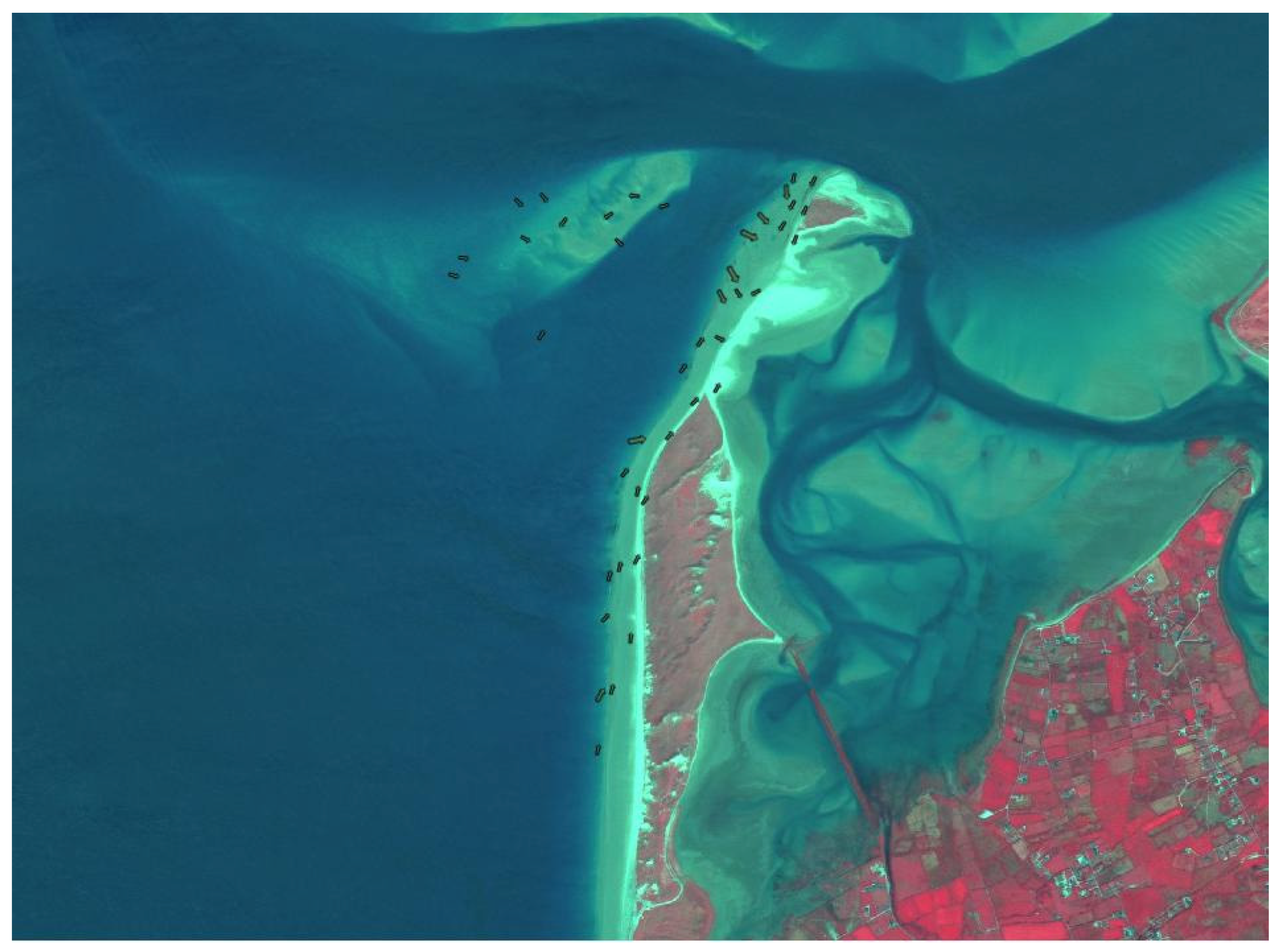
5.2. Comparison with Sediment Transport Simulations

As the GSTA sampling was undertaken during the modeling time period, direct comparisons of sediment transport results from both methods were possible. This presented a rare opportunity to assess the suitability of the GSTA method against a fully validated numerical morphodynamic model.
The modelled sediment transport regime was compared to the GSTA best case, CP−, Figure 9. A corresponding plot of modelled accumulated sediment transport over the same time period as the GSTA is represented in Figure 13.
Along the drift aligned dune section both GSTA and modelled sediment transport displayed alongshore and offshore wave dominated transport vectors. Although magnitude was notional in the GSTA analysis, the CP− case tended to display wave driven sediment transport as the dominant mode along the entire dune line of the drift aligned beach where as the modelled transport vectors displayed intermittent wave dominant sediment transport.
An interesting feature was the agreement at the Island terminus, where the sediment transport vectors appeared to be acting against the flood tidal current patterns and moving in an ebb tidal direction. Given the agreement of both numerical modelling derived sediment transport vectors and the GSTA trends, it was possible that this location may be ebb tidally dominated. This was a significant finding; given the nature of the bar migration described in O’Shea & Murphy [16]. The large sediment transport vectors explain why the ebb tidal bar migration was fastest at this location.
Comparing the trend analysis plot, it was evident that there were discrepancies between the two in certain areas of the coastal cell. The direction of accumulated sediment transport on the ebb tidal bar differs in direction with the modelled. The modelled sediment transport vectors appeared to be driven in the same direction as peak tidal flood currents while the GSTA trend vectors follow a direct shore normal route. This suggests that the GSTA method showed a bias for wave dominated sediment transport in this area.
The other area of disagreement was at the breached inlet on the drift aligned beach. The model results show strong sediment transport going east wards through the breach but the GSTA trends were in the opposite direction showing sediment transport moving offshore in a westerly direction. This can be explained again by the mode of dominant sediment transport the GSTA method was biased towards. The GSTA adopted a wave dominant transport mode for this location, describing the sediment transport driven by wave erosive at the breach, while the model shows tidal current sediment transport through the breach was dominant.

6. Further Work

While this study focused on Rossbeigh beach, it is acknowledged that further sampling over a larger regular grid to investigate fully the nature of Inner Dingle Bay pathway trends would be beneficial. A follow-up larger scale, multi seasonal sediment sampling and analysis campaign is recommended.

7. Conclusions

It was evident from the analysis in the previous section that the simulated and GSTA derived plots show good agreement. While discrepancies exist between the two the general trend of sediment transport in the study area described by numerical modelling results was reproduced by the GSTA method. This result provided further evidence there is merit in applying trend based methodologies to coastal sediment transport scenarios.

Acknowledgments

The authors would like to thank the CMRC and the Department of Geography in U.C.C., and in particular Jeremy Gault for the use of equipment during this research. They would also like to acknowledge the advice received from Max Kozyachenko and Emmanuel Poizot, on sediment analysis.

Author Contributions

Michael O’Shea and Jimmy Murphy conceived and designed the experiments; Michael O’Shea performed the experiments; Michael O’Shea analyzed the data; Michael O’Shea wrote the paper.

Conflicts of Interest

The authors declare no conflict of interest.

References

  1. December Ordinary Meeting Minutes; Kerry County Council: County Kerry, Ireland, 2009; p. 58.
  2. High Tides Bring Food Threat. The Kerrys Eye, 11 November 2010; 8.
  3. Krumbein, W.C.; Pettijohn, F.J. Manual of Sedimentary Petrography; Appleton-Century-Crofts: New York, NY, USA, 1938. [Google Scholar]
  4. McLaren, P. An interpretation of trends in grain size measures. J. Sediment. Res. 1981, 51, 611–624. [Google Scholar]
  5. Gao, S.; Collins, M. Net sediment transport patterns inferred from grain-size trends, based upon definition of “transport vectors”. Sediment. Geol. 1992, 80, 47–60. [Google Scholar] [CrossRef]
  6. LeRoux, J.P. An alternative approach to the identification of the end sediment transport paths based on grain size trends. Sediment. Geol. A 1994, 94, 97–107. [Google Scholar] [CrossRef]
  7. Poulos, S.; Ballay, A. Grain-size trend analysis for the determination of non-biogenic sediment transport pathways on the Kwinte Bank (southern North Sea), in relation to sand dredging. J. Coast. Res. 2010, 51, 87–92. [Google Scholar]
  8. Poizot, E.; Méar, Y. ECSedtrend: A new software to improve sediment trend analysis. Comput. Geosci. 2008, 34, 827–837. [Google Scholar] [CrossRef]
  9. Poizot, E.; Méar, Y. Using a GIS to enhance grain size trend analysis. Environ. Model. Softw. 2010, 25, 513–525. [Google Scholar] [CrossRef]
  10. Sala, P. Morphodynamic Evolution of a Tidal Inlet Mid-bay Barrier System. Master’s Thesis, University College Cork, Cork, Ireland, 2010. [Google Scholar]
  11. Vial, T. Monitoring the Morphological Response of an Embayed High Energy Beach To Storms and Atlantic Waves. Master’s Thesis, University College Cork, Cork, Ireland, 2008. [Google Scholar]
  12. Saini, S.; Jackson, N.L.; Nordstrom, K.F. Depth of activation on a mixed sediment beach. Coast. Eng. 2009, 56, 788–791. [Google Scholar] [CrossRef]
  13. Blott, S.J.; Pye, K. GRADISTAT: A grain size distribution and statistics package for the analysis of unconsolidated sediments. Earth Surf. Process. Landf. 2001, 26, 1237–1248. [Google Scholar] [CrossRef]
  14. DHI. MIKE 21: Sediment Transport and Morphological Modelling—User Guide; DHI Water and Environment: Hørsholm, Denmark, 2007; p. 388. [Google Scholar]
  15. Van Rijn, L.C. Principles of Coastal Morphology; Aqua Publications: Amsterdam, The Netherlands, 1998. [Google Scholar]
  16. O’Shea, M.; Murphy, J. Predicting and Monitoring the Evolution of a Coastal Barrier Dune System Postbreaching. J. Coast. Res. 2013, 29, 38–50. [Google Scholar] [CrossRef]
Figure 1. Study Area.
Jmse 04 00027 g001
Figure 2. Sediment sample locations.
Jmse 04 00027 g002
Figure 3. Average Grainsize Distribution of Site.
Jmse 04 00027 g003
Figure 4. Model Domain.
Jmse 04 00027 g004
Figure 5. Recorded and simulated tidal current velocity in drift aligned zone.
Jmse 04 00027 g005
Figure 6. Modelled vs. recorded Tz in Dingle Bay.
Jmse 04 00027 g006
Figure 7. Modelled vs. recorded Hs in Dingle Bay.
Jmse 04 00027 g007
Figure 8. Volume comparison locations.
Jmse 04 00027 g008
Figure 9. CP− trend.
Jmse 04 00027 g009
Figure 10. CB+ trend.
Jmse 04 00027 g010
Figure 11. FB+ trend.
Jmse 04 00027 g011
Figure 12. FP− trend.
Jmse 04 00027 g012
Figure 13. Simulated Accumulated Sediment transport vectors for Grain Size Trend Analysis (GSTA) comparison.
Jmse 04 00027 g013
Table 1. Sediment Sample Statistics.
LocationEastingNorthingMean ( x ¯ φ ) Sorting (σɸ)Skewness (SKɸ)
04641915944261.8610.411−0.028
14636855945561.9560.406−0.020
24638315945301.9060.413−0.033
34646535948932.2060.407−0.013
44647875948512.0220.370−0.013
54645355948072.0500.369−0.013
64645835946821.9590.405−0.023
74644585945932.0060.367−0.020
84643335947772.0200.369−0.008
94646865950012.1590.365−0.009
104636075946401.9940.404−0.015
114638775946142.1090.382−0.006
124641585946992.0510.383−0.013
134641275948602.2340.368−0.013
144642405948852.2290.369−0.019
154641775945712.0090.365−0.004
164642305942652.0110.613−0.600
17464484.6592379.52.0150.607−0.640
18464496.9592623.32.0060.516−0.148
19464551.4592652.22.1470.410−0.009
20464636.15926901.9770.492−0.052
21464638.2592885.31.3100.7360.040
22464596592915.82.0700.486−0.044
23464520.1592982.31.8960.537−0.146
24464540.8593167.81.8320.593−0.282
25464589.6593205.32.1110.406−0.013
26464659.6593243.81.9200.445−0.011
27464703.3593510.71.8690.483−0.050
28464668.2593553.91.8550.512−0.066
29464612.2593637.61.9270.515−0.130
30464666.8593782.71.8470.471−0.041
31464734.2593791.22.0850.441−0.007
32464809.7593804.11.7440.662−0.256
33464578.3592351.62.0550.450−0.030
34464630.9592321.41.9120.450−0.015
35464928.4593964.51.8690.445−0.019
36464906.4594048.31.8290.533−0.139
37464875.5594113.21.7140.559−0.158
38464957.2594230.41.9000.445−0.019
39465038.2594243.71.9650.447−0.033
40465050.7594439.21.8830.453−0.037
41465124.4594457.51.9030.481−0.050
42465201.9594462.51.8970.453−0.012
43465024.3594020.21.9110.404−0.001
44465146.6594132.21.8760.406−0.012
45465266.6594427.51.8790.409−0.010
46465320.9594581.31.7620.498−0.015
47465380.5594697.21.9180.409−0.009
48465505.65949321.8080.451−0.019
49465465.9594966.41.7810.529−0.256
50465376.7594976.21.9660.427−0.029
51465343.1594912.41.8440.513−0.101
52465367594857.71.7280.574−0.120
53465423594829.41.9150.446−0.022
54465328.4594761.71.7590.505−0.058
55465234.4594793.41.8030.578−0.366
56465177.4594719.71.8790.587−0.318
57465213.4594656.91.7870.455−0.042
58465184.55945501.6800.467−0.044
59465099.8594539.72.0170.475−0.049
Table 2. Summary stats by location.
Dmean (µm)
TotalBarSwashDrift
Max297287274297
Min210220210220
Avg255252243260
Sorting (σ)
TotalBarSwashDrift
Max150140137150
Min57576068
Avg88739292
Skewness (SKa)
TotalBarSwashDrift
Max4.164.094.162.89
Min0.660.660.730.71
Avg1.10.91.391.11
Table 3. Final model parameter values.
ModuleParameterValue
HDEddy Viscosity—Smagorinsky0.28
Bed Resistance (Manning)32 m3·s−1
STPorosity0.4
grain size0.25
Bank erosion slope failure30 Deg angle of repose
SWSpectralFully spectral
TimeInterstationary
Spectral discretisation25 frequencies, min of 0.055 Hz
Directional discretisation16 over 360 Deg rose
Wave breakingGamma of 0.8 Alpha 1
White capping4.5—constant
Directional Spreading Index4
Table 4. Volume comparison of morphodynamic simulations.
LocationCut (m3)Fill (m3)Balance (m3)
ChannelSurvey
−6021212010659894
Model
−6921011469745487

