
Modeling Storm Surge and Inundation in Washington, DC, during Hurricane Isabel and the 1936 Potomac River Great Flood

Abstract
:1. Introduction
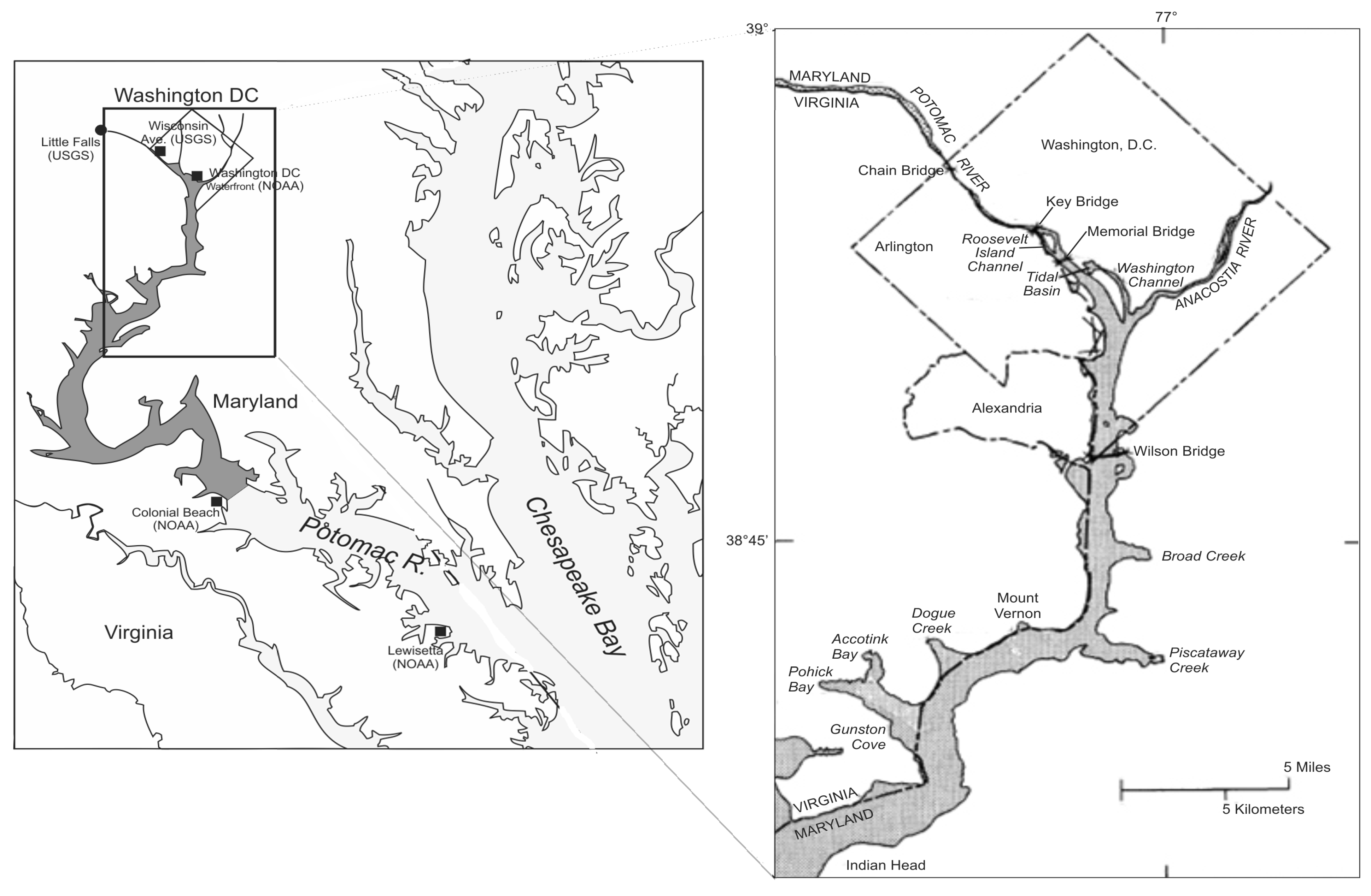
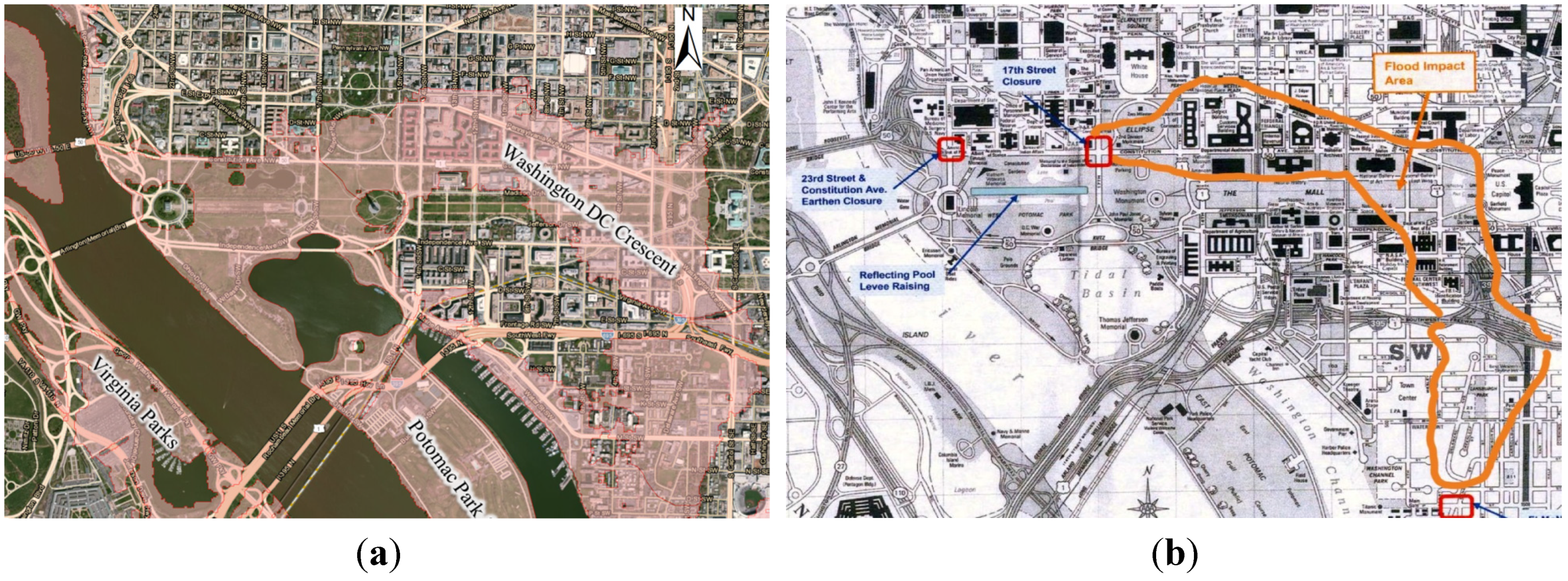
2. Study Area
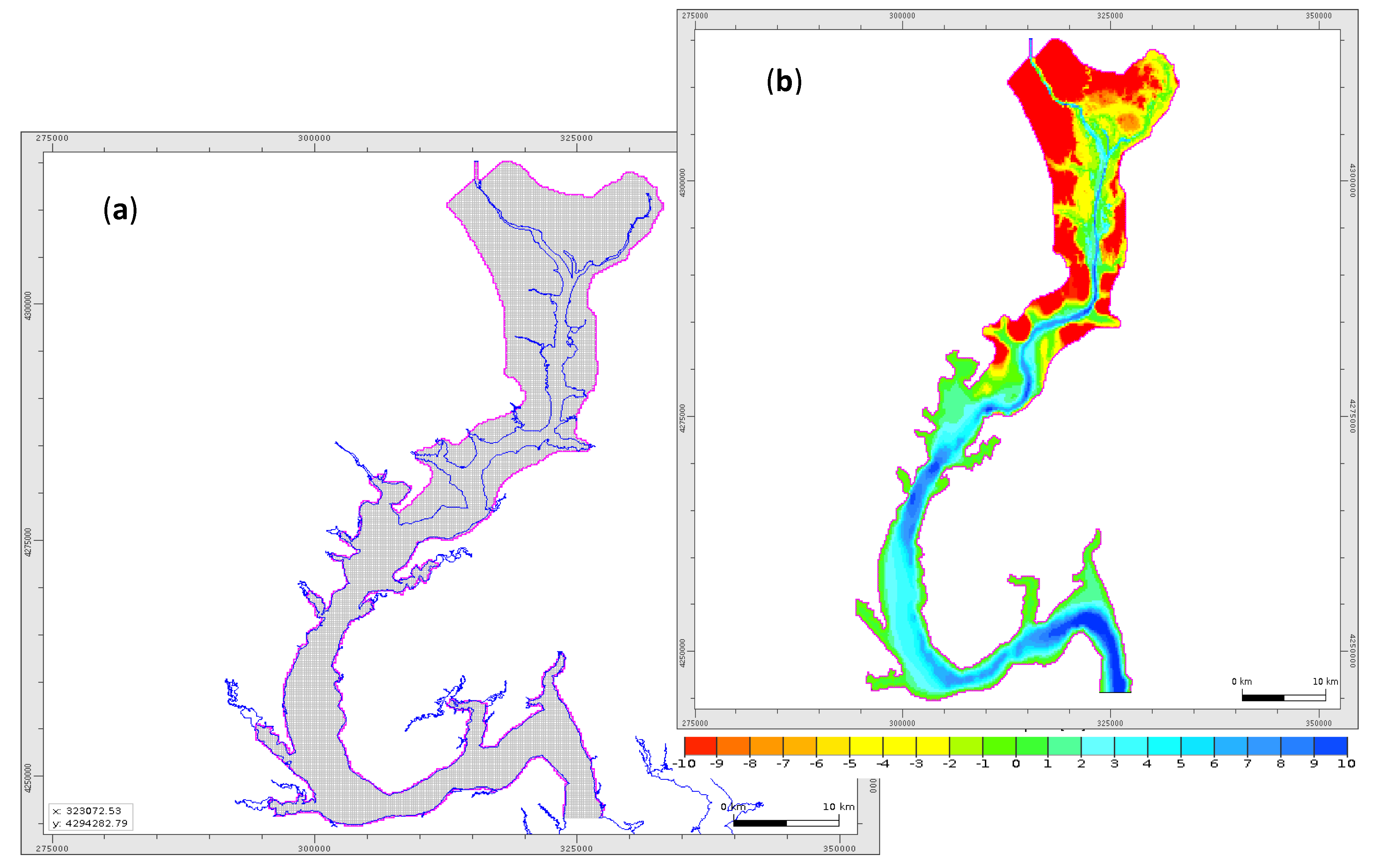
3. Storm Surge and Inundation Model Incorporating Sub-Grids in the Upper Tidal Potomac River
3.1. Model Description
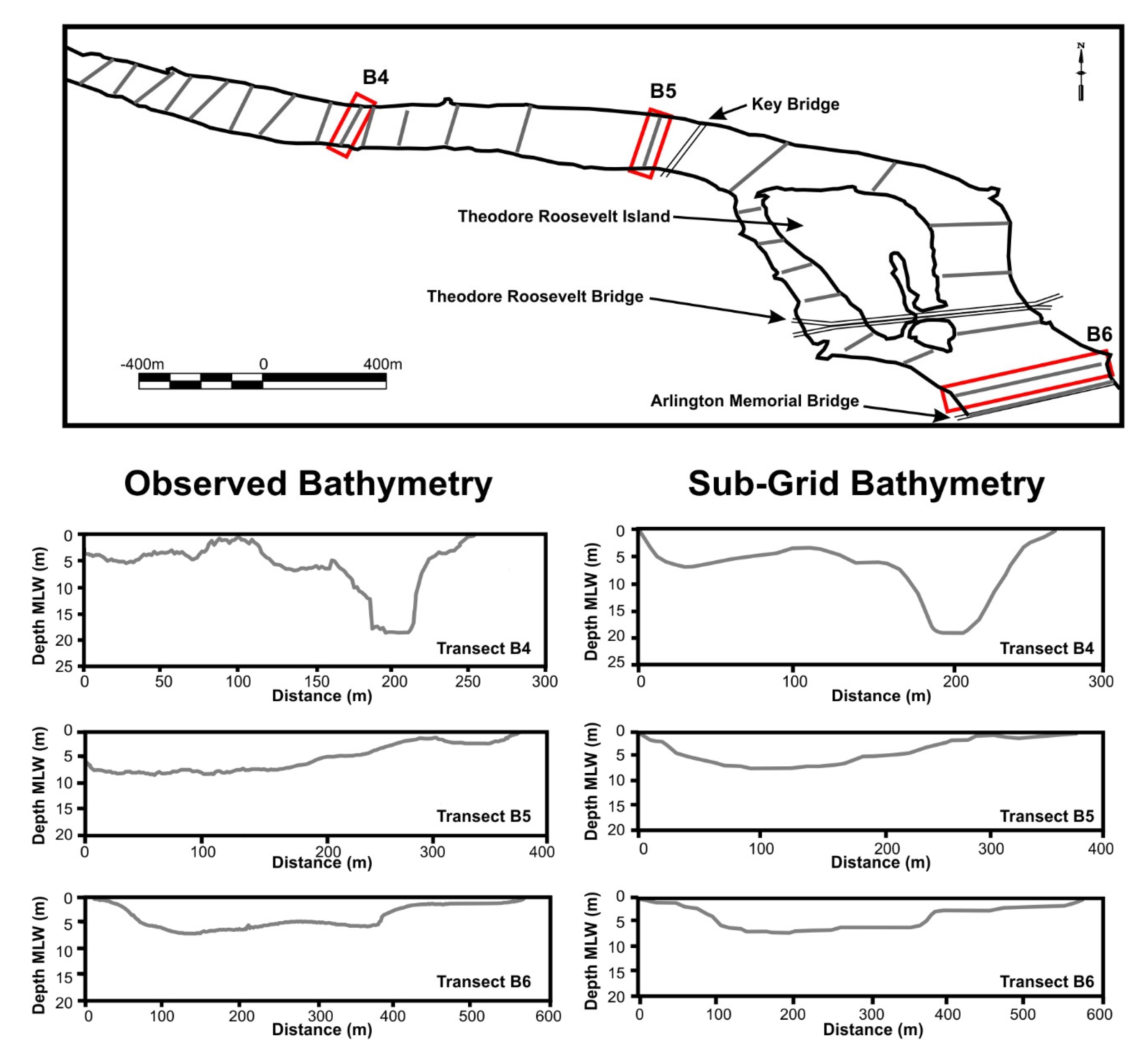
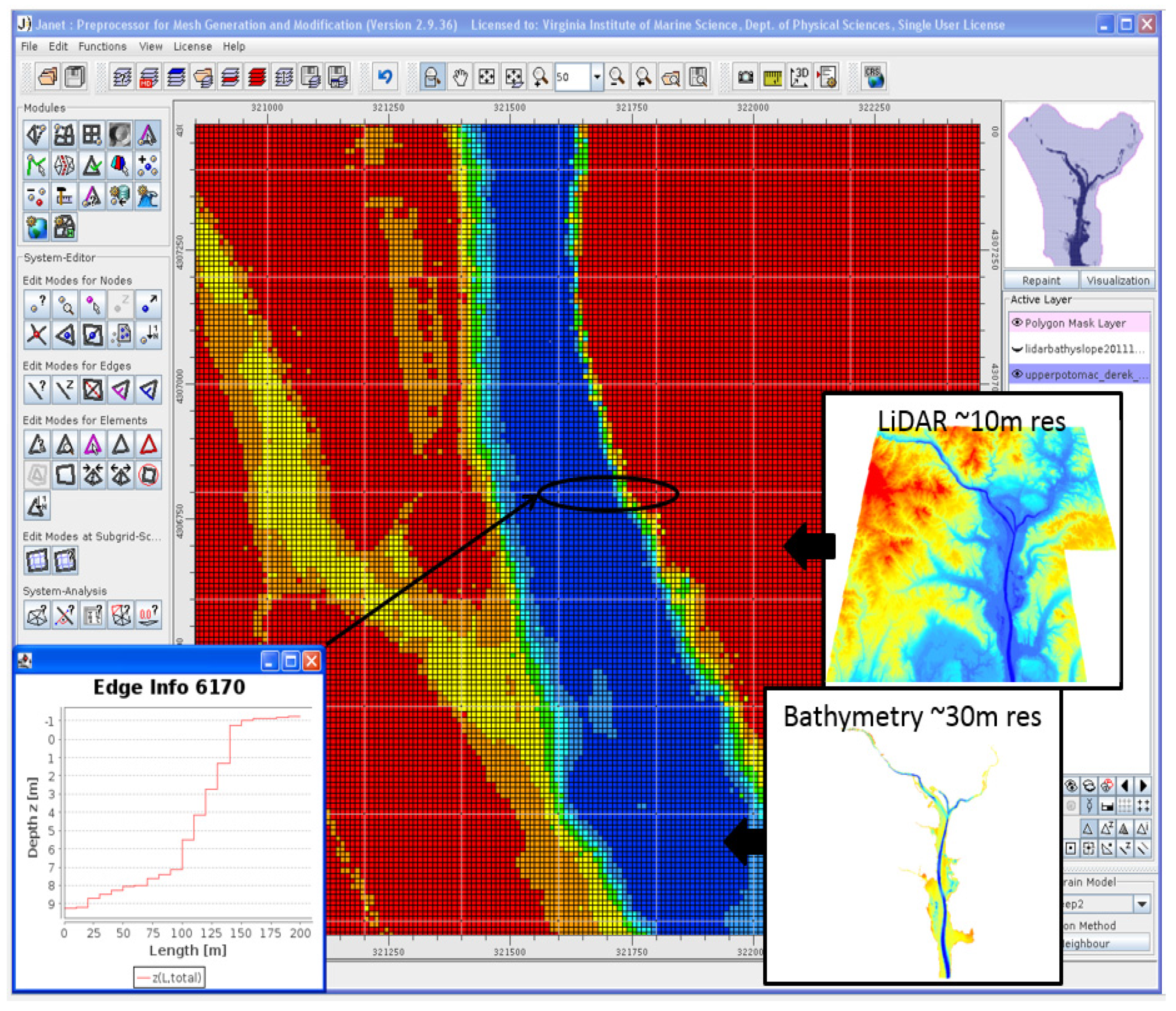
3.2. Incorporation of LiDAR-Derived DEM into the Sub-Grid Model Domain


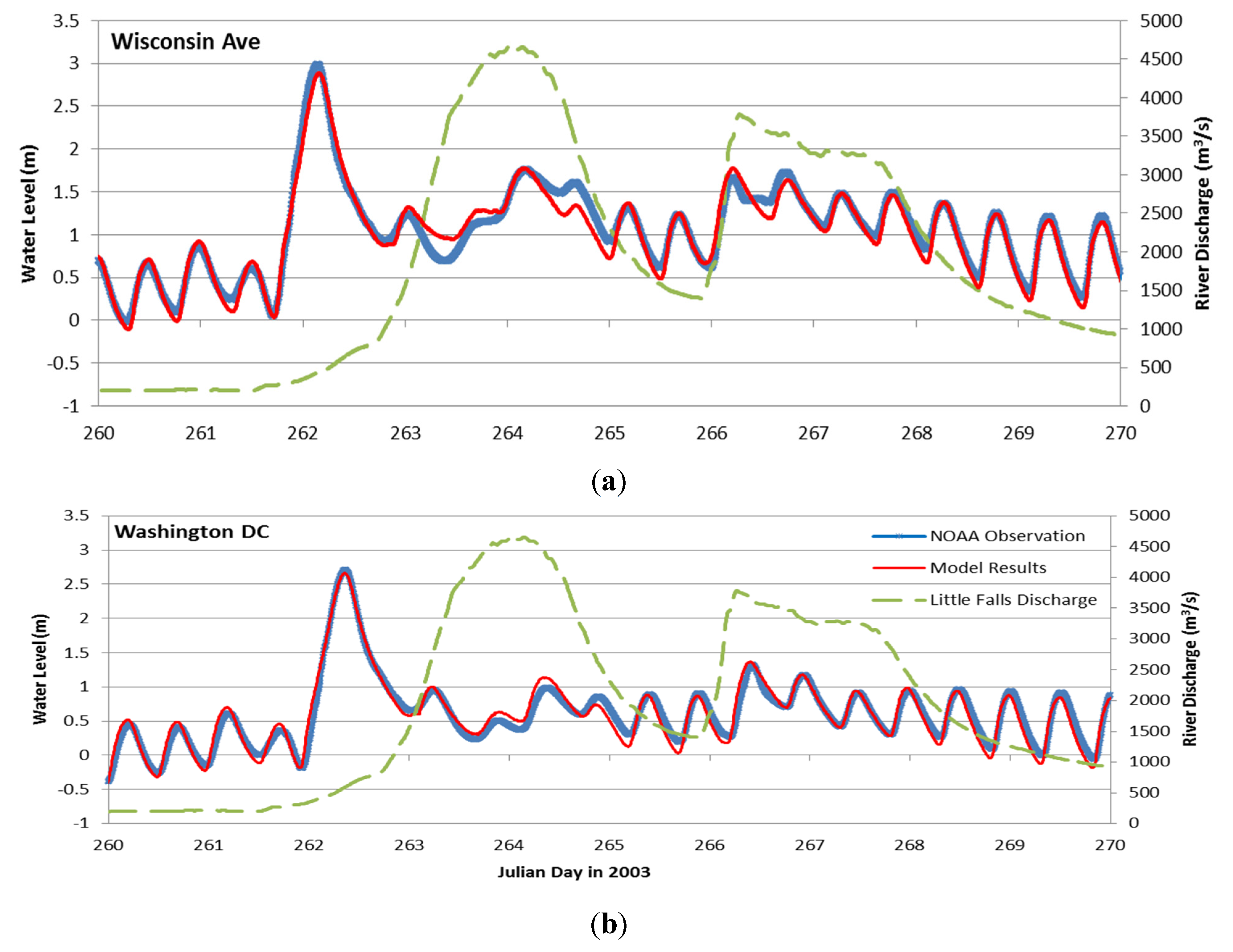
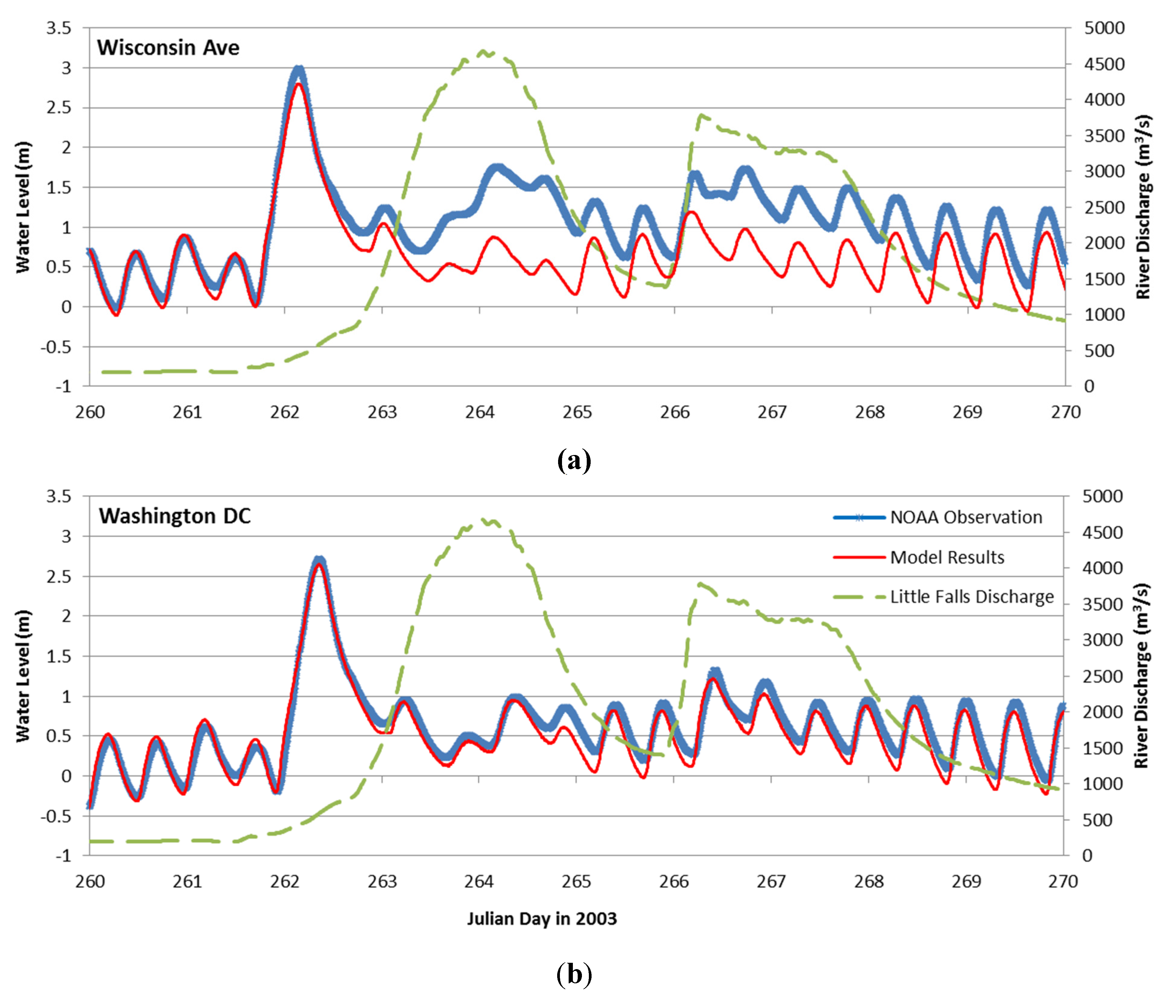
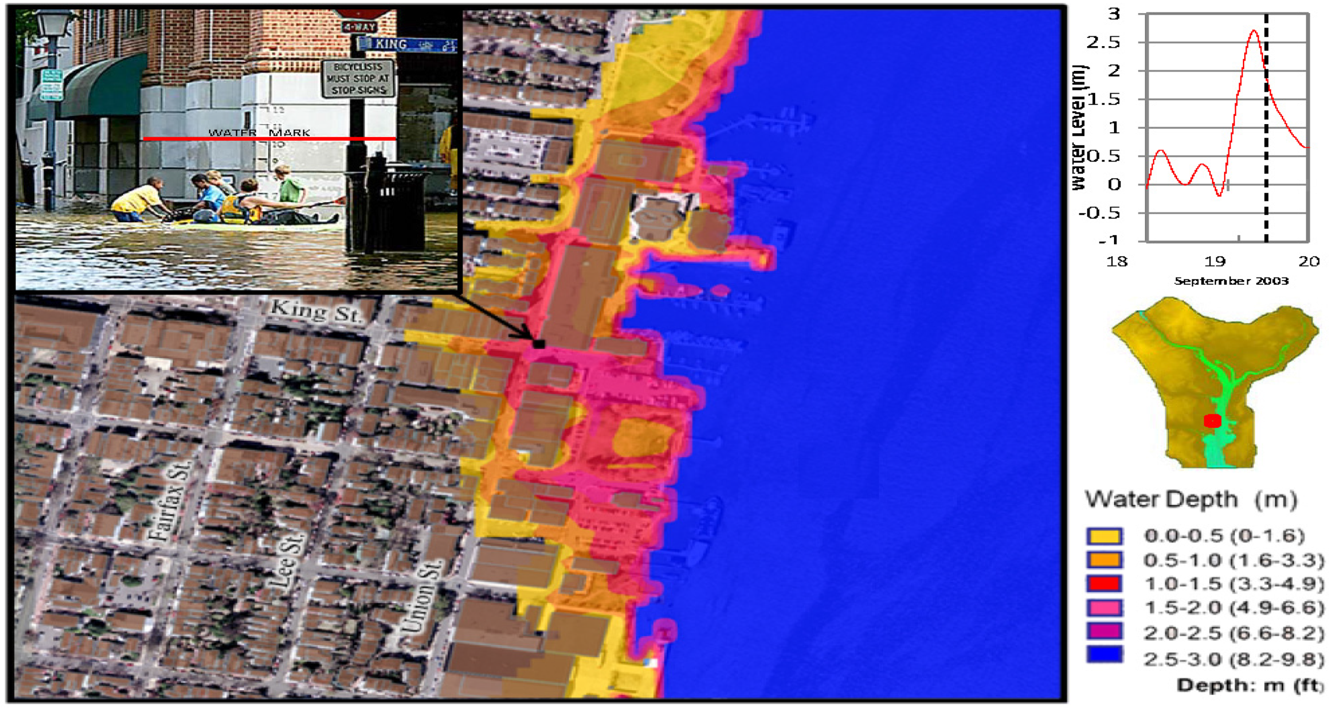
4. Modeling the 2003 Hurricane Isabel Event
4.1. Model Setup
4.2. Results

| Statistic | Wisconsin Ave. | Washington, DC |
|---|---|---|
| R² | 0.94 | 0.98 |
| RMS | 14.3 cm | 7.3 cm |
| MAE | 11.4 cm | 4.8 cm |
| Peak Difference | 9.2 cm | 2.4 cm |

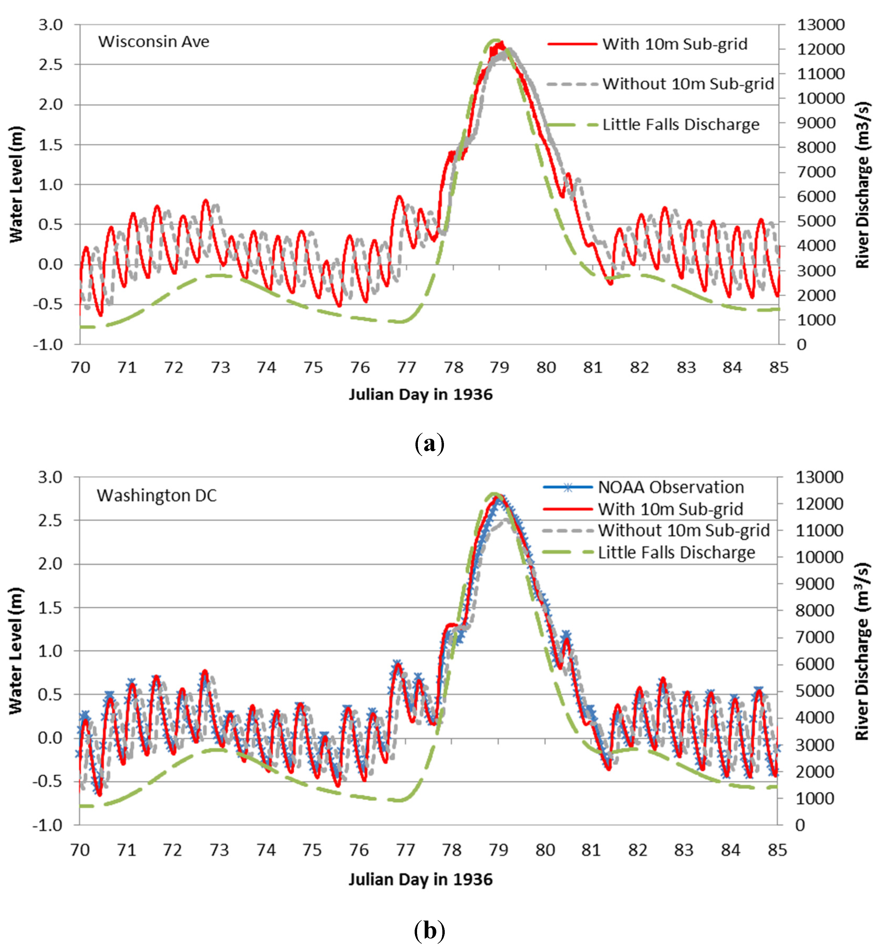
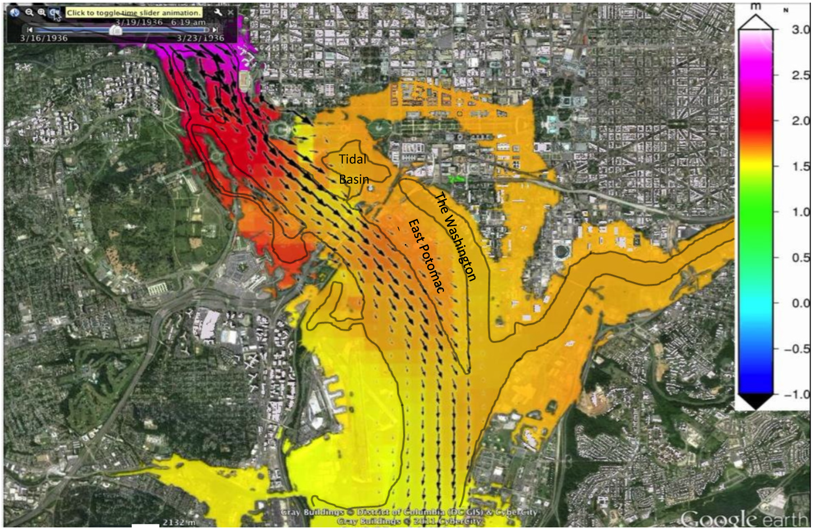
5. Inundation Simulation for the Potomac River Great Flood of 1936
5.1. Model Setup
5.2. Results

| Statistic | “With” Sub-Grid | “Without” Sub-Grid |
|---|---|---|
| R2 | 0.98 | 0.77 |
| RMS | 5.8 cm | 41.0 cm |
| MAE | 3.7 cm | 36.0 cm |
| Peak Difference | 2.9 cm | 23.8 cm |

| Modeled Flood Area | m2 | km2 | mi2 |
|---|---|---|---|
| Potomac Park & Golf Course | 3,118,210.81 | 3.12 | 1.20 |
| Washington DC Crescent * | 2,466,778.05 | 2.47 | 0.95 |
| Washington Harbor | 1,167,493.83 | 1.17 | 0.45 |
| DC Naval Yard | 633,843.92 | 0.63 | 0.24 |
| Reagan Airfield | 1,819,267.96 | 1.82 | 0.70 |
| Virginia Parks | 1,778,806.55 | 1.78 | 0.69 |
| Anacostia-Bolling Base & Park | 1,632,464.54 | 1.63 | 0.63 |
| Total | 12,616,865.65 | 12.62 | 4.87 |
| * DC Crescent Modeled Flood Area | m2 | km2 | mi2 |
| Upper Crescent | 1,815,294.67 | 1.82 | 0.70 |
| Lower Crescent | 651,483.375 | 0.65 | 0.25 |
| Total | 2,466,778.05 | 2.47 | 0.95 |
6. Discussion and Conclusions
Acknowledgments
Author Contributions
Conflicts of Interest
Abbreviations
| USACE | US Army Corps of Engineers, Department of Defense |
| NOAA Co-OPS | National Oceanic and Atmospheric Administration, Center for Operational Oceanographic Products and Services |
| NAVD88 | North America vertical datum of 1988 |
| NAD83 CORS96 | North America datum of 1983, readjusted based on the Continuous Operating Reference Stations (CORS) |
References
- Heaps, N.S. On the numerical solution of the three-dimensional hydrodynamic equations for tides and storm surge. Mem. Soc. R. Soc. Sci. Liėge Coll Huit 1972, 2, 143–180. [Google Scholar]
- Reid, R.O.; Bodin, R.O. Numerical model for storm surges in Galveston Bay. J. Waterw. Harbor Div. 1968, 94, 33–57. [Google Scholar]
- Davis, A.M. Three-dimensional modelling of surge. In Flood due to High Winds and Tides; Peregrine, D.H., Ed.; Academic Press: London, UK, 1981; pp. 45–74. [Google Scholar]
- Jelesnianski, C.P.; Chen, J.; Shaffer, W.A. SLOSH: Sea, Lake, and Overland Surges from Hurricanes; National Weather Service: Silver Spring, MD, USA, 1992. [Google Scholar]
- Kerr, P.C.; Donahue, A.S.; Westerink, J.J.; Luettich, R.A., Jr.; Zheng, L.Y.; Weisberg, R.H.; Huang, Y.; Wang, H.V.; Teng, Y.; Forrest, D.R.; et al. US IOOS coastal and ocean modeling testbed: Inter-model evalulation of tides, waves, and hurricane surge in the Gulf of Mexico. J. Geophys. Res. 2013, 118, 5129–5172. [Google Scholar]
- Chen, C.; Beardsley, R.C.; Luettich, R.A., Jr.; Westerink, J.J.; Wang, H.; Perrie, W.; Xu, Q.; Donahue, A.S.; Qi, J.; Lin, H.; et al. Extratropical storm inundation testbed: Intermodel comparisons in Situate, Massachusetts. J. Geophys. Res. Oceans 2013, 118, 5054–5073. [Google Scholar]
- Roland, Aron; Zhang, Y.; Wang, H.V.; Meng, Y.; Teng, Y.; Maderichd, V.; Brovchenkod, I.; Dutour-Sikirice, M.; Zankea, U. A fully coupled 3D wave-current interaction model on unstructured grids. JGR Oceans 2012, 117, C00J33. [Google Scholar] [CrossRef]
- Neelz, S.; Pender, G. Sub-gird scale parameterisation of 2D hydrodynamic models of inundation in the urban area. Acta Geophys. 2007, 55, 65–72. [Google Scholar] [CrossRef]
- Casas, A.S.; Lane, N.; Yu, D.; Benito, G. A method for parameterizing roughness and topographic sub-grid scale effects in hydraulic modelling from LiDAR data. Hydrol. Earth Syst. Sci. Discuss. 2010, 7, 2261–2299. [Google Scholar]
- Wang, H.V.; Loftis, J.D.; Liu, Z.; Forrest, D.; Zhang, J. The storm surge and sub-grid inundation modeling in New York City during Hurricane Sandy. J. Mar. Sci. Eng. 2014, 2, 226–246. [Google Scholar]
- United States Geological Survey (USGS). Part3. Potomac, James, and Upper Ohio Rivers (Water-Supply Paper 800). In The floods of March 1936; United States Geological Survey: Denver, CO, USA, 1937. [Google Scholar]
- Schaffranek, R. A Flow Simulation Model of the Tidal Potomac River—A Water-Quality Study of the Tidal Potomac River and Estuary; United States Geological Survey: Denver, CO, USA, 1987; p. 2234-D. [Google Scholar]
- Mashriqui, H.S.; Halgren, J.S.; Reed, S.M. Toward Modeling of river-estuary-ocean interactions to enhance operational river forecasting in the NOAA National Weather Service. In Proceedings of the 2nd Joint Federal Interagency Conference, Las Vegas, NV, USA, 27 June–1 July 2010.
- EA Engineering, Science, and Technology, Inc. Water Quality Studies in the Vicinity of the Washington Aqueduct; Baltimore District, US Army Corps of Engineers, Washington Aqueduct Division: Washington, DC, USA, October 2001. [Google Scholar]
- Casulli, V. A semi-implicit finite difference method for non-hydrostatic, free-surface flows. Int. J. Numer. Methods Fluids 1999, 30, 425–440. [Google Scholar] [CrossRef]
- Casulli, V.; Walters, R.A. An unstructured grid, three-dimensional model based on the shallow water equations. Int. J. Numer. Methods Fluids 2000, 32, 331–348. [Google Scholar] [CrossRef]
- Casulli, V.; Zanolli, P. High resolution methods for multidimensional advection-diffusion problems in free-surface hydrodynamics. Ocean Model. 2005, 10, 137–151. [Google Scholar] [CrossRef]
- Casulli, V. A high-resolution wetting and drying algorithm for free-surface hydrodynamics. Int. J. Numer. Methods Fluid Dyn. 2009, 60, 391–408. [Google Scholar] [CrossRef]
- Casulli, V.; Stelling, G. Semi-implicit sub-grid modeling of three-dimensional free-surface flows. Int. J. Numer. Methods Fluid Dyn. 2011, 67, 441–449. [Google Scholar] [CrossRef]
- Loftis, J.D.; Wang, H.V.; Hamilton, S.E.; Forrest, D.R. Combination of LiDAR Elevations, Bathymetric Data, and Urban Infrastructure in a Sub-Grid Model for Predicting Inundation in New York City during Hurricane Sandy. Comput. Environ. Urban Syst. 2015. under review. [Google Scholar]
- Casulli, V.; Zanolli, P. A three-dimensional semi-implicit algorithm for environmental flows on unstructured grids. In Proceedings of the Conference on Methods for Fluid Dynamics, University of Oxford, Oxford, UK; 1998; pp. 57–70. [Google Scholar]
- Hederson, F.M. Open Channel Flow. 1996; The Macmillan Company: New York, NY, USA; p. 522.
- Garratt, J.R. Review of drag coefficients over oceans and continents. Mon. Weather Rev. 1977, 105, 915–929. [Google Scholar] [CrossRef]
- Powell, M.D.; Vickery, P.J.; Reinhold, T.A. Reduced drag coefficient for high wind speeds in tropical cyclones. Nature 2003, 422, 279–283. [Google Scholar] [CrossRef] [PubMed]
- Stamey, B.; Wang, H.V.; Koterba, M. Predicting the Next Storm Surge Flood. Sea Technol. 2007, 48, 10–15. [Google Scholar]
- Arnold, J.L. The Evolution of the Flood Control Act of 1936; United States Army Corps of Engineers: Fort Belvoir, VR, USA, 1988. [Google Scholar]
- VIMS Physical Science. 1936 Potomac River flood simulation. Available online: http://web.vims.edu/physical/3DECM/DC19360301/ (accessd on 11 July 2015).
- National Capital Planning Commission (NCPC). Flooding and Stormwater in Washington, DC, 2008. Available online: http://www.ncpc.gov/DocumentDepot/Publications/FloodReport2008.pdf (accessed on 17 January 2008).
- Loftis, J.D.; Wang, H.V.; DeYoung, R.J.; Ball, W.B. Integrating LiDAR Data into a High-Resolution Topo-bathymetric DEM for Use with Sub-Grid Inundation Modeling at NASA Langley Research Center. J. Coast. Res. 2015, in press. [Google Scholar]
- Loftis, J.D. Development of a Large-Scale Storm Surge and High-Resolution Sub-Grid Inundation Model for Coastal Flooding Applications: A Case Study during Hurricane Sandy. Ph.D. Thesis, College of William & Mary, Williamsburg, VA, USA, 2014. [Google Scholar]
- Smith, W. Climate Change Symposium, Washington Metropolitan Council of Governments, May 21, 2012. Available online: http://www.mwcog.org/environment/climate/adaptation/Presentations/5-%20Smith.pdf (accessed on 22 May 2012).
© 2015 by the authors; licensee MDPI, Basel, Switzerland. This article is an open access article distributed under the terms and conditions of the Creative Commons Attribution license ( http://creativecommons.org/licenses/by/4.0/).
Share and Cite
Wang, H.V.; Loftis, J.D.; Forrest, D.; Smith, W.; Stamey, B. Modeling Storm Surge and Inundation in Washington, DC, during Hurricane Isabel and the 1936 Potomac River Great Flood. J. Mar. Sci. Eng. 2015, 3, 607-629. https://doi.org/10.3390/jmse3030607
Wang HV, Loftis JD, Forrest D, Smith W, Stamey B. Modeling Storm Surge and Inundation in Washington, DC, during Hurricane Isabel and the 1936 Potomac River Great Flood. Journal of Marine Science and Engineering. 2015; 3(3):607-629. https://doi.org/10.3390/jmse3030607
Chicago/Turabian StyleWang, Harry V., Jon Derek Loftis, David Forrest, Wade Smith, and Barry Stamey. 2015. "Modeling Storm Surge and Inundation in Washington, DC, during Hurricane Isabel and the 1936 Potomac River Great Flood" Journal of Marine Science and Engineering 3, no. 3: 607-629. https://doi.org/10.3390/jmse3030607
APA StyleWang, H. V., Loftis, J. D., Forrest, D., Smith, W., & Stamey, B. (2015). Modeling Storm Surge and Inundation in Washington, DC, during Hurricane Isabel and the 1936 Potomac River Great Flood. Journal of Marine Science and Engineering, 3(3), 607-629. https://doi.org/10.3390/jmse3030607