
Wind and Wave Setup Contributions to Extreme Sea Levels at a Tropical High Island: A Stochastic Cyclone Simulation Study for Apia, Samoa

Abstract
:
1. Introduction
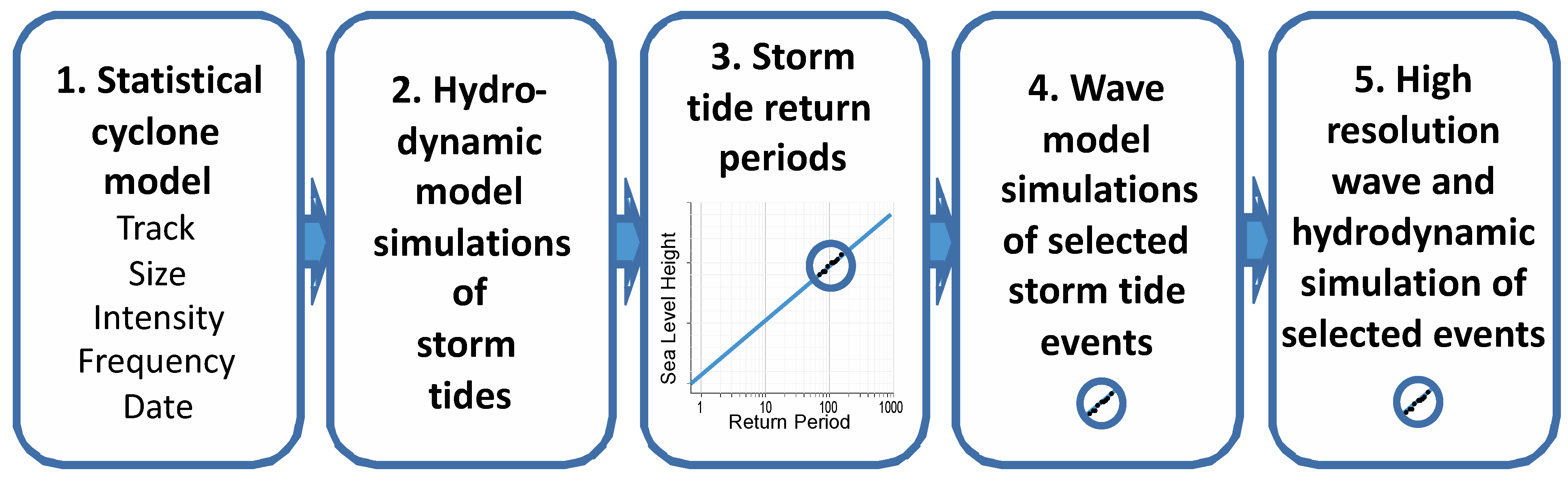
2. Experimental Section
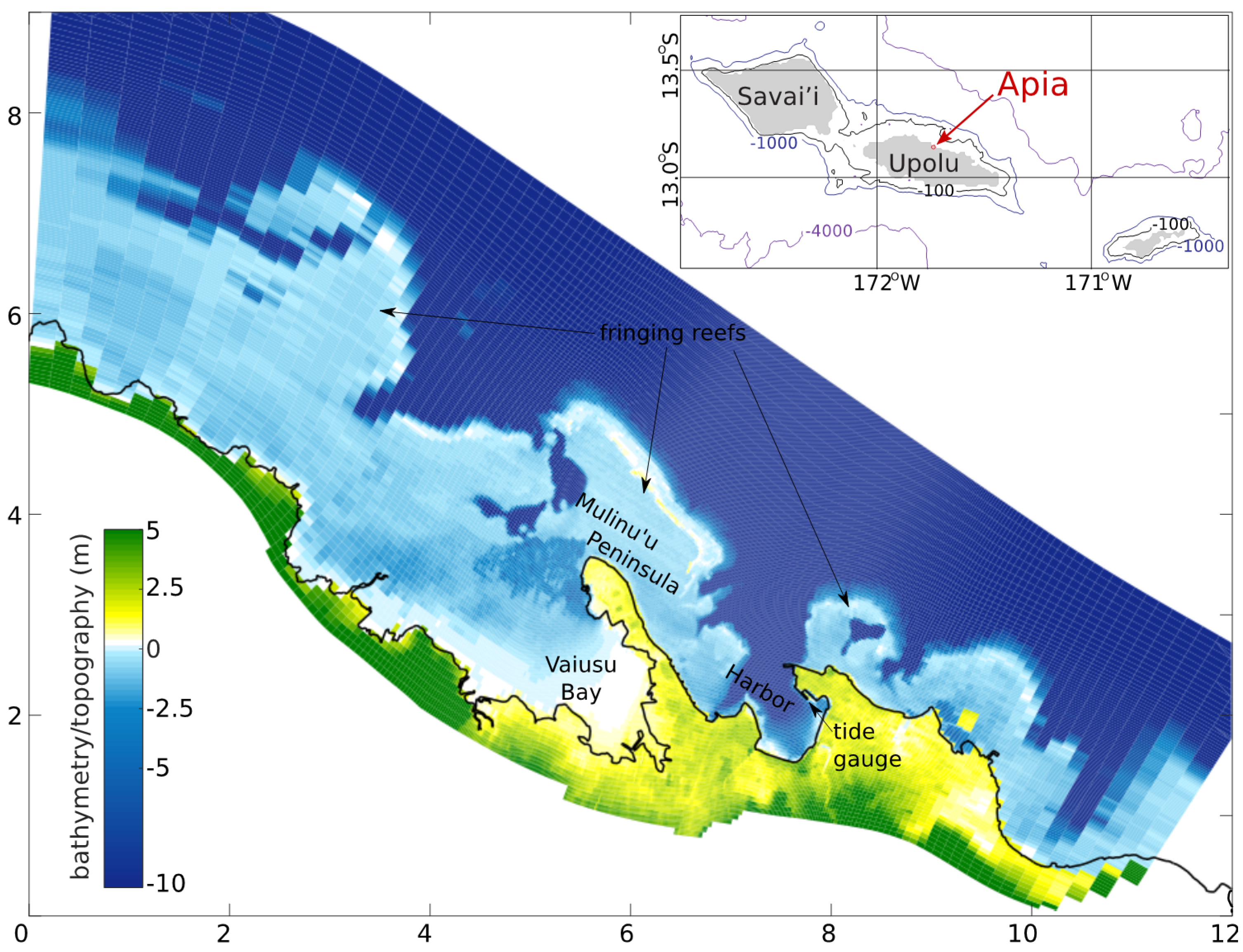
2.1. Study Site and Context
2.2. Ensemble Methodology


2.3. Model Implementation
2.3.1. Archipelago Wave Model
2.3.2. Apia Model
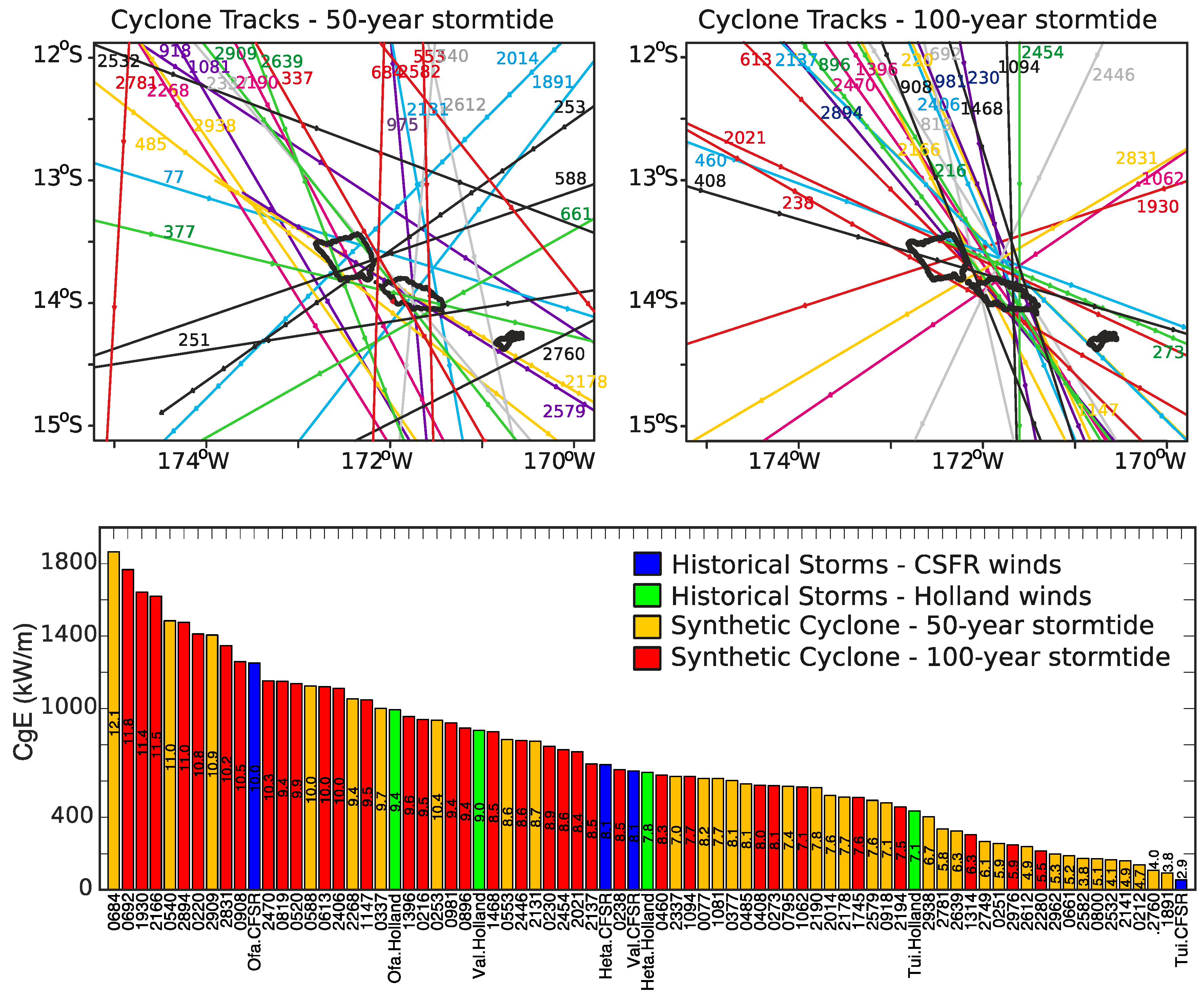
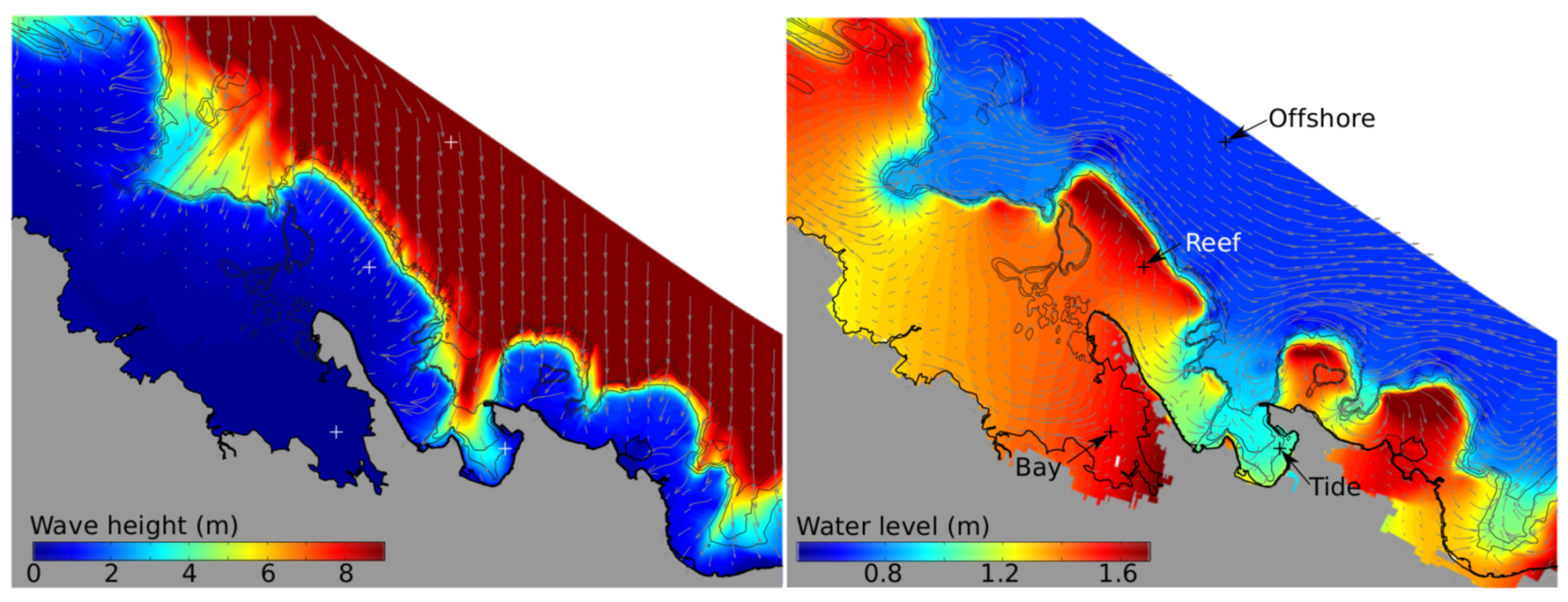
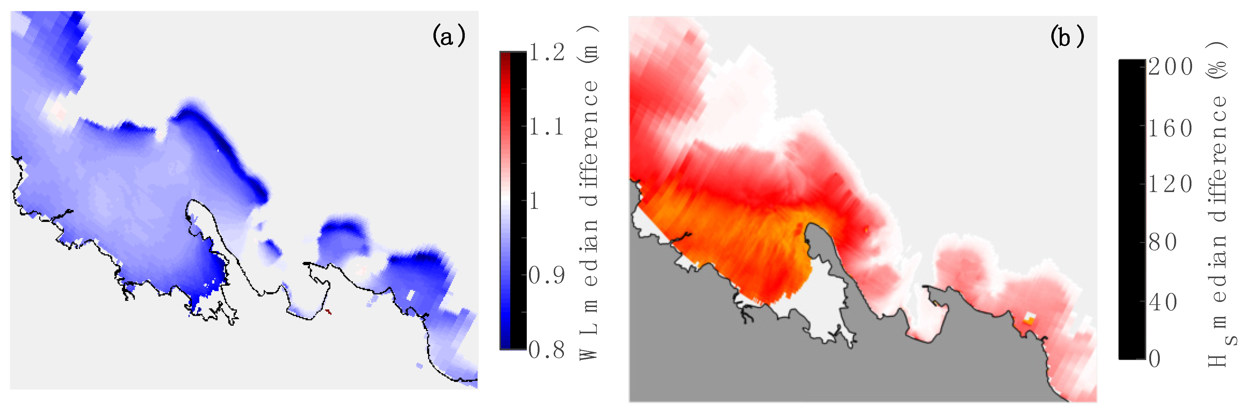
3. Results
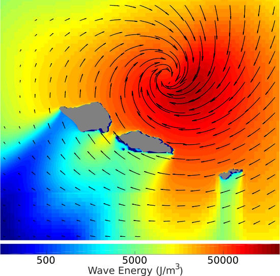
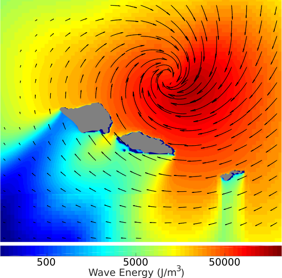
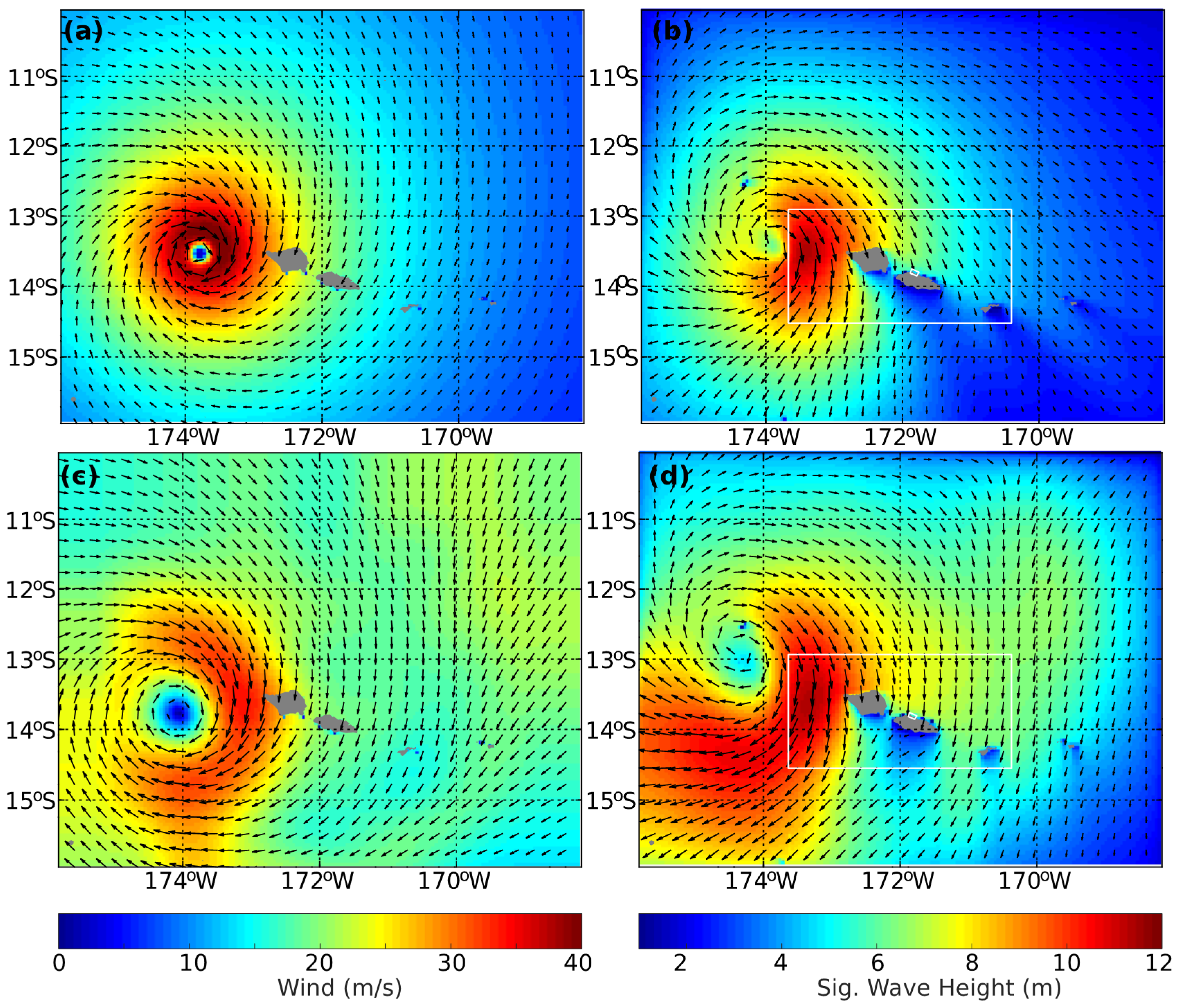
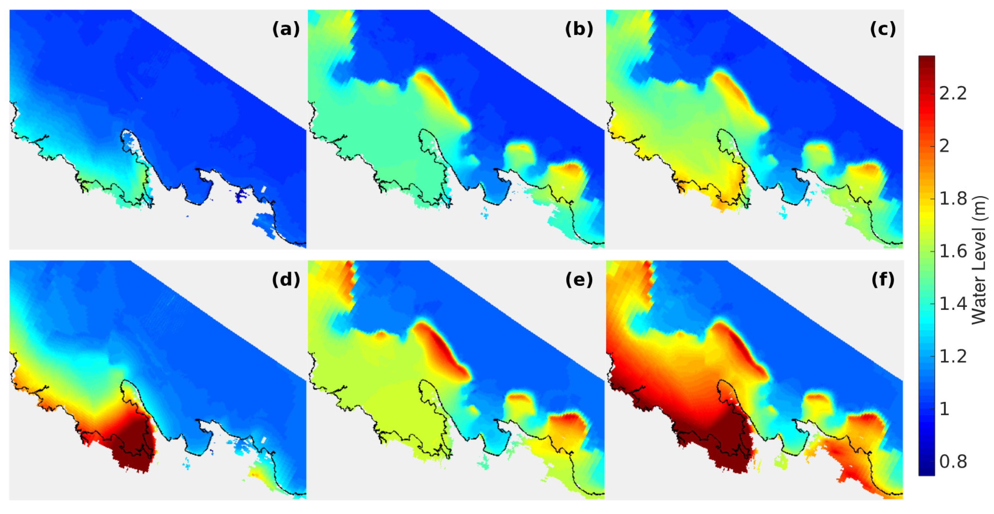
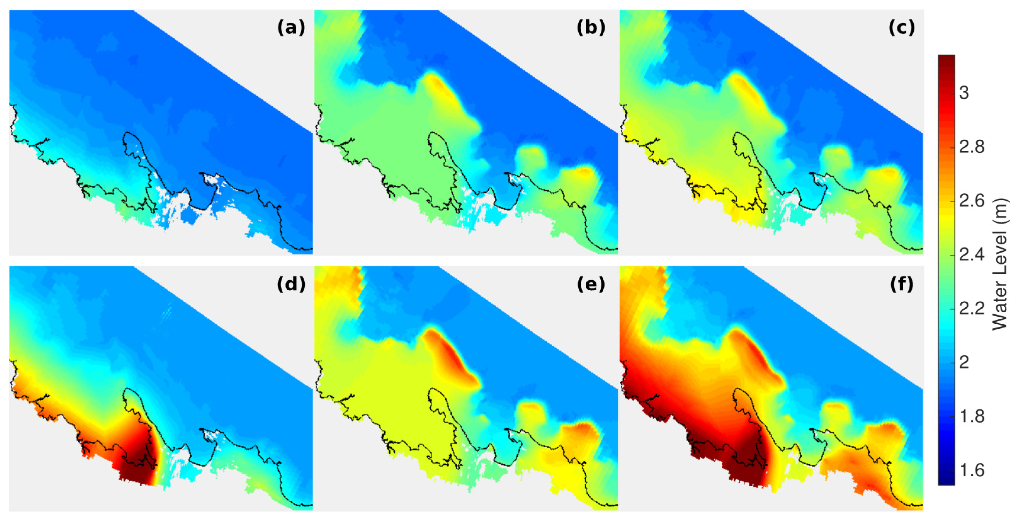
3.1. Archipelago Wave Model Results
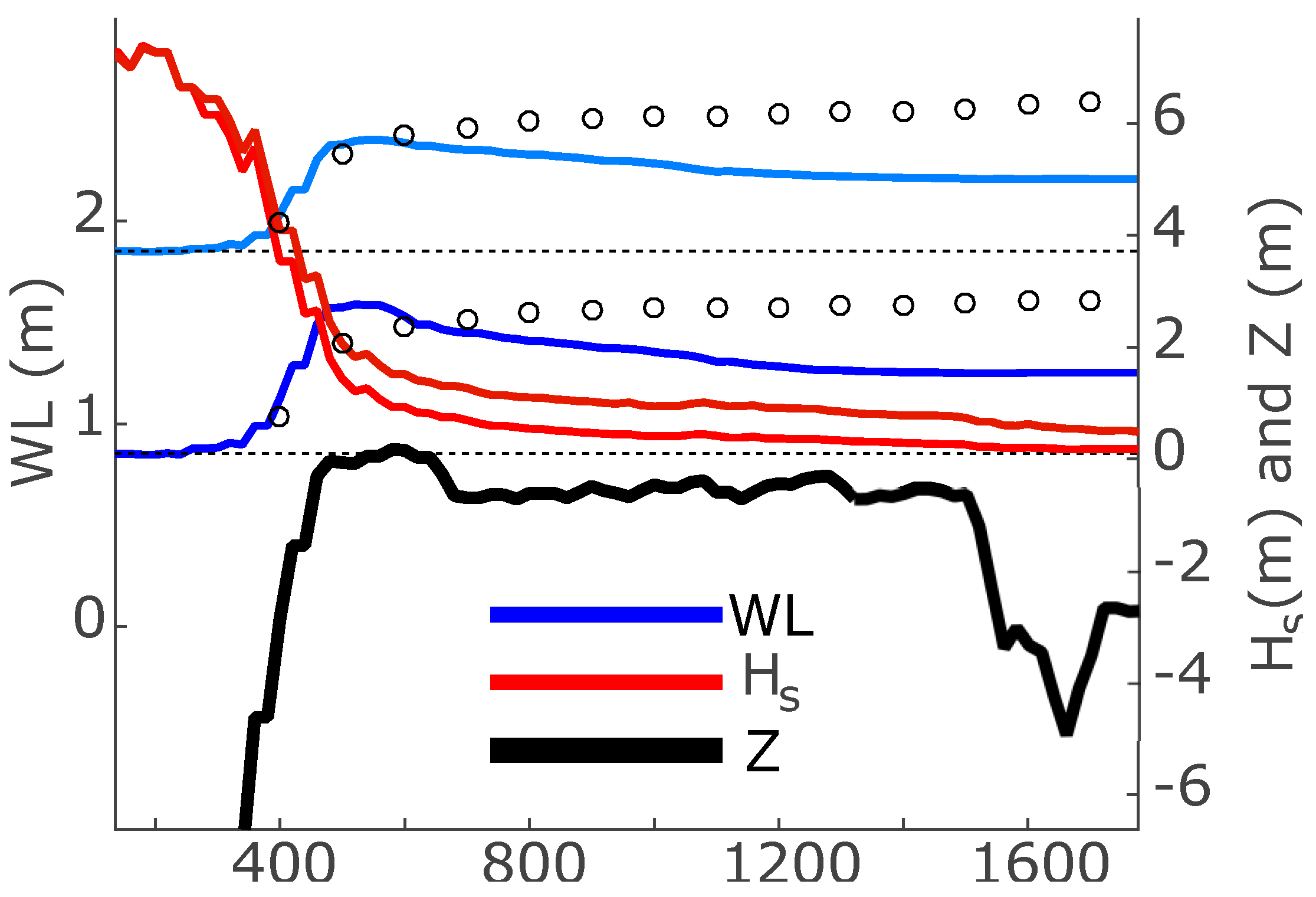
3.2. Apia Model Results


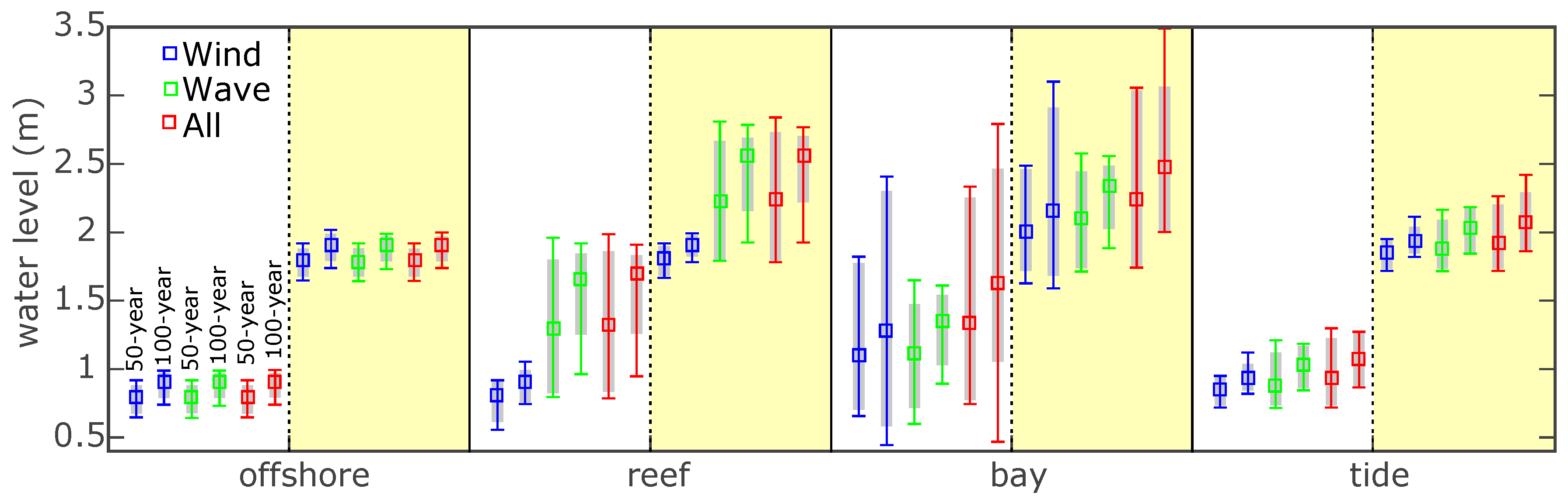
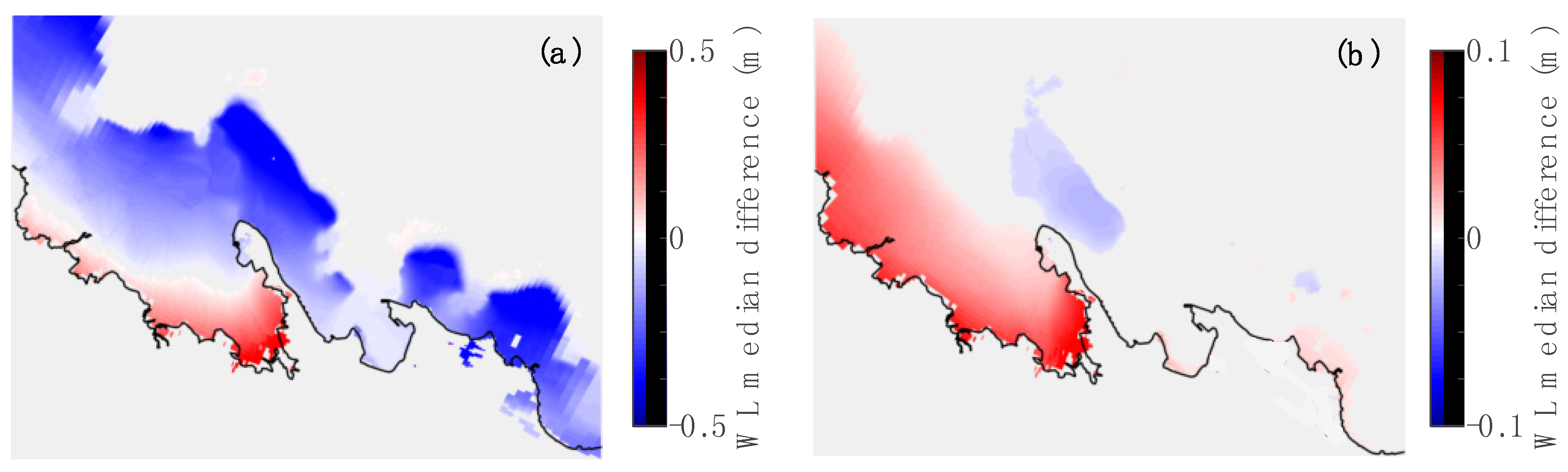
4. Discussion

5. Conclusions
Acknowledgments
Conflicts of Interest
References
- Diamond, H.J.; Lorrey, A.M.; Knapp, K.R.; Levinson, D.H. Development of an enhanced tropical cyclone tracks database for the southwest Pacific from 1840 to 2010. Int. J. Climatol. 2011, 32, 2240–2250. [Google Scholar] [CrossRef]
- Stephens, S.A.; Ramsay, D.L. Extreme cyclone wave climate in the Southwest Pacific Ocean: Influence of the El Niño Southern Oscillation and projected climate change. Glob. Planet Chang. 2014, 123, 13–26. [Google Scholar] [CrossRef]
- McInnes, K.L.; Walsh, K.J.E.; Hoeke, R.K.; O’Grady, J.G.; Colberg, F.; Hubbert, G.D. Quantifying storm tide risk in Fiji due to climate variability and change. Glob. Planet Chang. 2014, 116, 115–129. [Google Scholar] [CrossRef]
- Pugh, D.T. Changing Sea Levels: Effects of Tides, Weather and Climate; Cambridge University Press: Cambridge, UK, 2004. [Google Scholar]
- Hubbert, G.D.; Mclnnes, K.L. A Storm Surge Inundation Model for Coastal Planning and Impact Studies. J. Coast. Res. 1999, 15, 168–185. [Google Scholar]
- Kennedy, A.B.; Westerink, J.J.; Smith, J.M.; Hope, M.E.; Hartman, M.; Taflanidis, A.A.; Tanaka, S.; Westerink, H.; Fai, K.; Smith, T.; et al. Tropical cyclone inundation potential on the Hawaiian Islands of Oahu and Kauai. Ocean Model. 2012, 52–53, 54–68. [Google Scholar] [CrossRef]
- Hoeke, R.K.; Mcinnes, K.L.; Kruger, J.C.; Mcnaught, R.J.; Hunter, J.R.; Smithers, S.G. Widespread inundation of Pacific islands triggered by distant-source wind-waves. Glob. Planet Chang. 2013, 108, 128–138. [Google Scholar] [CrossRef]
- Vetter, O.; Becker, J.; Merrifield, M.; Pequignet, A.; Aucan, J.; Boc, S.; Pollock, C. Wave setup over a Pacific Island fringing reef. J. Geophys. Res. 2010, 115, 1–13. [Google Scholar] [CrossRef]
- Merrifield, M.A.; Becker, J.M.; Ford, M.; Yao, Y. Observations and estimates of wave-driven water level extremes at the Marshall Islands. Geophys. Res. Lett. 2014, 41, 7245–7253. [Google Scholar] [CrossRef]
- Walsh, K.J.E.; McInnes, K.L.; McBride, J.L. Climate change impacts on tropical cyclones and extreme sea levels in the South Pacific—A regional assessment. Glob. Planet Chang. 2012, 80–81, 149–164. [Google Scholar] [CrossRef]
- McInnes, K.L.; Hoeke, R.K.; Walsh, K.J.E.; O’Grady, J.G.; Hubbert, G.D. Application of a Synthetic Cyclone Method for Assessment of Tropical Cyclone Storm Tides in Samoa. Nat. Hazards 2015, 79. [Google Scholar] [CrossRef]
- Hoeke, R.; McInnes, K.; O’Grady, J.; Lipkin, F.; Colberg, F. High Resolution Met-Ocean Modelling for Storm Surge Risk Analysis in Apia, Samoa; CAWCR: Melbourne, Australia, 2014; Volume 71, pp. 1–80. [Google Scholar]
- Mulligan, R.P.; Hay, A.E.; Bowen, A.J. Wave-driven circulation in a coastal bay during the landfall of a hurricane. J. Geophys. Res. 2008, 113. [Google Scholar] [CrossRef]
- Australian Bureau of Meteorology and CSIRO. Climate Variability, Extremes and Change in the Western Tropical Pacific: New Science and Updated Country Reports; Australian Bureau of Meteorology and CSIRO: Melbourne, Australia, 2014.
- Durrant, T.; Greenslade, D.; Hemer, M.; Trenham, C. A Global Wave Hindcast focussed on the Central and South Pacific; CAWCR: Melbourne, Australia, 2014. [Google Scholar]
- Ready, S.; Woodcock, F. The South Pacific and southeast Indian Ocean tropical cyclone season 1989–1990. Aust. Meteorol. Mag. 1992, 40, 111–121. [Google Scholar]
- Gill, J.P. The South Pacific and southeast Indian Ocean tropical cyclone season 1991–1992. Aust. Meteorol. Mag. 1994, 43, 181–192. [Google Scholar]
- Solomon, S.M. A Review of Coastal Processes and Analysis of Historical Coastal Change in the Vinicity of Apia, Western Samoa; South Pacific Applied Geoscience Commission: Suva, Fiji, 1994; Volume 208, p. 62. [Google Scholar]
- Bureau of Meteorology, Samoa. Available online: http://www.bom.gov.au/pacific/samoa (accessed on 18 September 2015).
- Rearic, D.M. Survey of Cyclone Ofa Damage to the Northern Coast of Upolu, Western Samoa; South Pacific Applied Geoscience Commission: Suva, Fiji, 1990; Volume 104, p. 36. [Google Scholar]
- Carter, R. Design of the Seawall for Mulinu’u Point, Western Samoa; South Pacific Applied Geoscience Commission: Suva, Fiji, 1987; Volume 78, p. 30. [Google Scholar]
- Holland, G. A Revised Hurricane Pressure-Wind Model. Mon. Weather Rev. 2008, 136, 3432–3445. [Google Scholar] [CrossRef]
- Booij, N.; Ris, R.C.; Holthuijsen, L.H. A third-generation wave model for coastal regions 1. Model description and validation. J. Geophys. Res. 1999, 104, 7649–7666. [Google Scholar] [CrossRef]
- Wu, J. Wind-stress coefficients over sea surface from breeze to hurricane. J. Geophys. Res. 1982, 87, 9704. [Google Scholar] [CrossRef]
- Huang, Y.; Weisberg, R.H.; Zheng, L.; Zijlema, M. Gulf of Mexico hurricane wave simulations using SWAN: Bulk formula-based drag coefficient sensitivity for Hurricane Ike. J. Geophys. Res. 2013, 118, 3916–3938. [Google Scholar] [CrossRef]
- Zijlema, M.; van Vledder, G.P.; Holthuijsen, L.H. Bottom friction and wind drag for wave models. Coast. Eng. 2012, 65, 19–26. [Google Scholar] [CrossRef]
- Janssen, P.A.E.M. Wave-Induced Stress and the Drag of Air Flow over Sea Waves. J. Phys. Oceanogr. 1989, 19, 745–754. [Google Scholar] [CrossRef]
- Saha, S.; Moorthi, S.; Wu, X.; Wang, J.; Nadiga, S.; Tripp, P.; Behringer, D.; Hou, Y.-T.; Chuang, H.; Iredell, M.; et al. The NCEP Climate Forecast System Version 2. J. Clim. 2014, 27, 2185–2208. [Google Scholar] [CrossRef]
- Lesser, G.R.; Roelvink, J.A.; van Kester, J.A.T.M.; Stelling, G.S. Development and validation of a three-dimensional morphological model. Coast. Eng. 2004, 51, 883–915. [Google Scholar] [CrossRef]
- Mulligan, R.P.; Walsh, J.P.; Wadman, H.M. Storm surge and surface waves in a shallow lagoonal estuary during the crossing of a hurricane. J. Waterw. Port. Coast. Ocean Eng. 2015, 141, A5014001. [Google Scholar] [CrossRef]
- Barnard, P.L.; van Ormondt, M.; Erikson, L.H.; Eshleman, J.; Hapke, C.; Ruggiero, P.; Adams, P.N.; Foxgrover, A.C. Development of the Coastal Storm Modeling System (CoSMoS) for predicting the impact of storms on high-energy, active-margin coasts. Nat. Hazards 2014, 74, 1095–1125. [Google Scholar] [CrossRef]
- Taebi, S.; Pattiaratchi, C. Hydrodynamic response of a fringing coral reef to a rise in mean sea level. Ocean Dyn. 2014, 64, 975–987. [Google Scholar] [CrossRef]
- Hoeke, R.K.; Storlazzi, C.D.; Ridd, P. V Drivers of circulation in a fringing coral reef embayment: A wave-flow coupled numerical modeling study of Hanalei Bay, Hawaii. Cont. Shelf Res. 2013, 58, 79–95. [Google Scholar] [CrossRef]
- Roelvink, J.A.; Walstra, D.-J. Ro keeping it simple bu using complex models. Adv. Hydro-Sci. Eng. 2004, 6, 1–11. [Google Scholar]
- Lowe, R.J.; Falter, J.L.; Bandet, M.D.; Pawlak, G.; Atkinson, M.J.; Monismith, S.G.; Koseff, J.R. Spectral wave dissipation over a barrier reef. J. Geophys. Res. 2005, 110, 1–16. [Google Scholar] [CrossRef]
- Filipot, J.-F.; Cheung, K.F. Spectral wave modeling in fringing reef environments. Coast. Eng. Proc. 2012, 67, 67–79. [Google Scholar] [CrossRef]
- Madsen, O.; Poon, Y.; Graber, H. Spectral Wave Attenuation by Bottom Friction: Theory. Coast. Eng. Proc. 1988, 21, 492–504. [Google Scholar]
- Raubennheimer, B.; Guza, R.T.; Elgar, S. Field observations of wave-driven setdown and setup. J. Geophys. Res. 2001, 106, 4629–4638. [Google Scholar] [CrossRef]
- Murakami, H. Tropical cyclones in reanalysis data sets. Geophys. Res. Lett. 2014, 41, 2133–2141. [Google Scholar] [CrossRef]
- Li, N.; Roeber, V.; Yamazaki, Y.; Heitmann, T.W.; Bai, Y.; Cheung, K.F. Integration of coastal inundation modeling from storm tides to individual waves. Ocean Model. 2014, 83, 26–42. [Google Scholar] [CrossRef]
- Hench, J. Episodic circulation and exchange in a wave-driven coral reef and lagoon system. Limnol. Oceanogr. 2008, 53, 2681–2694. [Google Scholar] [CrossRef]
- Taebi, S.; Lowe, R.J.; Pattiaratchi, C.B.; Ivey, G.N.; Symonds, G.; Brinkman, R. Nearshore circulation in a tropical fringing reef system. J. Geophys. Res. 2011, 116, C02016. [Google Scholar] [CrossRef]
- Gourlay, M.R.; Colleter, G. Wave-generated flow on coral reefs—An analysis for two-dimensional horizontal reef-tops with steep faces. Coast. Eng. 2005, 52, 353–387. [Google Scholar] [CrossRef]
- Becker, J.; Merrifield, M.A.; Ford, M. Water level effects on breaking wave setup for Pacific Island fringing reefs. J. Geophys. Res. 2014, 119, 914–932. [Google Scholar] [CrossRef]
- Andersson, A.J.; Gledhill, D. Ocean acidification and coral reefs: Effects on breakdown, dissolution, and net ecosystem calcification. Ann. Rev. Mar. Sci. 2013, 5, 321–348. [Google Scholar] [CrossRef] [PubMed]
- Grady, A.E.; Moore, L.J.; Storlazzi, C.D.; Elias, E.; Reidenbach, M.A. The influence of sea level rise and changes in fringing reef morphology on gradients in alongshore sediment transport. Geophys. Res. Lett. 2013, 40, 3096–3101. [Google Scholar] [CrossRef]
- Buckley, M.; Lowe, R.; Hansen, J. Evaluation of nearshore wave models in steep reef environments. Ocean. Dyn. 2014, 64, 847–862. [Google Scholar] [CrossRef]
- Pomeroy, A.; Lowe, R. The dynamics of infragravity wave transformation over a fringing reef. J. Geophys. Res. 2012, 117, C11022. [Google Scholar] [CrossRef]
- Péquignet, A.-C.N.; Becker, J.M.; Merrifield, M.A. Energy transfer between wind waves and low-frequency oscillations on a fringing reef, Ipan, Guam. J. Geophys. Res. 2014, 119, 6709–6724. [Google Scholar] [CrossRef]
© 2015 by the authors; licensee MDPI, Basel, Switzerland. This article is an open access article distributed under the terms and conditions of the Creative Commons Attribution license ( http://creativecommons.org/licenses/by/4.0/).
Share and Cite
Hoeke, R.K.; McInnes, K.L.; O’Grady, J.G. Wind and Wave Setup Contributions to Extreme Sea Levels at a Tropical High Island: A Stochastic Cyclone Simulation Study for Apia, Samoa. J. Mar. Sci. Eng. 2015, 3, 1117-1135. https://doi.org/10.3390/jmse3031117
Hoeke RK, McInnes KL, O’Grady JG. Wind and Wave Setup Contributions to Extreme Sea Levels at a Tropical High Island: A Stochastic Cyclone Simulation Study for Apia, Samoa. Journal of Marine Science and Engineering. 2015; 3(3):1117-1135. https://doi.org/10.3390/jmse3031117
Chicago/Turabian StyleHoeke, Ron Karl, Kathleen L. McInnes, and Julian G. O’Grady. 2015. "Wind and Wave Setup Contributions to Extreme Sea Levels at a Tropical High Island: A Stochastic Cyclone Simulation Study for Apia, Samoa" Journal of Marine Science and Engineering 3, no. 3: 1117-1135. https://doi.org/10.3390/jmse3031117
APA StyleHoeke, R. K., McInnes, K. L., & O’Grady, J. G. (2015). Wind and Wave Setup Contributions to Extreme Sea Levels at a Tropical High Island: A Stochastic Cyclone Simulation Study for Apia, Samoa. Journal of Marine Science and Engineering, 3(3), 1117-1135. https://doi.org/10.3390/jmse3031117