1. Introduction
Salt marshes are among the most productive ecosystems on Earth and provide a variety of ecosystem services, such as storm protection of coastal cities, nutrients removal, and carbon storage [
1,
2,
3]. In spite of their important services, salt marshes are continuously threatened by external forcing such as wave action, sea-level rise, decrease in sediment supply, and land reclamation. As a result, large salt marsh losses have been documented worldwide [
4,
5,
6,
7,
8]. Understanding salt marsh dynamics and morphological evolution is, thus, a key issue for society and a critical component for the correct management and preservation of these coastal wetlands.
Salt marshes have been found to be able to keep peace with sea-level rise and to be inherently stable along the vertical direction due to feedbacks between inundation, organic matter production, and vertical accretion [
9,
10]. On the contrary, they appear unstable along the horizontal direction and weak with respect to the action of wind waves due to the lack of feedbacks between processes leading to lateral erosion and those contributing to salt marsh expansion [
11,
12]. Marsh erosion due to wind-waves attack has long been recognized as a mechanism for marsh loss and many studies have focused on the qualitative description of edge erosion and mechanics, and/or quantifying erosion rates through time [
13,
14,
15,
16,
17,
18,
19,
20,
21].
The rate of erosion depends on several parameters, such as soil type, marsh platform elevation, vegetation, and macrofauna. For instance, Leonardi and Fagherazzi [
5,
6] showed that the presence of a local variability in soil resistance affects the shape of marsh boundaries and the large-scale morphodynamic response of salt marshes to wind waves. A field study in Galveston Bay, Texas, indicated that sites with clay soils eroded less than those with loamy soils [
15]. This is in agreement with wave-tank experiments conducted by Feagin
et al. [
22], in which they showed that marsh soils with higher sand content are more erodible, and found that one of the main mechanisms by which vegetation prevents erosion is by modifying soil parameters. Macrofauna can also affect the resistance of marsh boundaries. Vegetation grazing by crabs can trigger vegetation die-off on marsh banks reducing the overall bank stability [
23]. Burrowing by crabs also facilitates sediment removal and localized erosion [
24]. In some instances, lateral erosion of salt marshes has been directly linked to infestation by burrowing crustaceans [
25].
Hall
et al. [
15] also found that the passage of Hurricane Alicia (which made landfall 80 km from their study site) did very little to accelerate erosion, and concluded that high water levels brought by the storm surge protected the shoreline from edge erosion. This process was confirmed by Tonelli
et al. [
26] who demonstrated, using a high-resolution Boussinesq model, that wave forcing at marsh edges increases with water level up to the point when the marsh is submerged, and then it rapidly decreases. Therefore, boundary erosion primarily occurs in period of storminess when water level is around mean sea level and close to the marsh platform elevation.
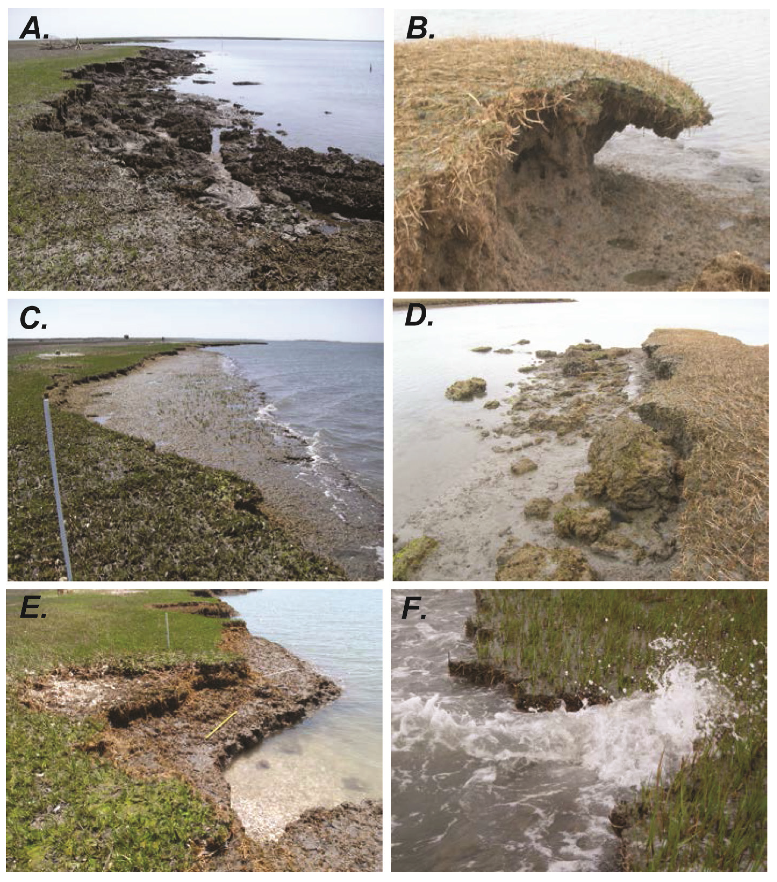
Figure 1.
Degradation of marsh scarps in Hog Island Bay, Virginia. The action of waves at lower water levels can remove previously eroded material (A) and cause undercutting (B); The process of root scalping occurs when waves attack the marsh at water levels approaching the marsh platform elevation (C); toppling is also common (D); Examples of wave gully: at low tide (E) and during a storm with wave energy concentration (F).
The erosion of salt marshes by wind waves can follow different styles, such as undercutting of the marsh scarp and consequent cantilever failure (
Figure 1B,D), as also reported by Allen [
19]. Waves tend to break offshore at low tide while also being small due to the limited water depth, which can result in a local lowering of the intertidal basin by removing previously eroded material (
Figure 1A). Wave-cut gullies [
27] are sub-triangular features that incise the marsh shoreline due to wave impact along scarped edges made of cohesive soils (
Figure 1E,F). These features were previously noted in the literature as “points” and “cuts” by Hall
et al. [
15] and “clefts” and “necks” by Schwimmer [
28]. Analysis of the hydrodynamics within a 10 m gully along the Louisiana coast revealed that run-up velocities increase at the gully head as a result of wave-crest compression owing to the gully’s convergent geometry [
27]. Because of the increased energy by wave concentration, erosion at the gully head is often three to five times greater than that at the shoreline [
27]. When waves occur at water elevations near that of the marsh platform, they may strike against the weak boundary separating the live vegetation root layer from the peat layer, which occurs at about 20 cm depth. The upward force of the impinging waves was observed in the field to torque the root mat upward, which results in uprooting and removal of the active root layer, a process termed “root-scalping” (
Figure 1C). Marsh boundary erosion can also be caused by crabs that excavate burrows in the vegetation substrate, thus, removing material and weakening the bank [
24,
25].
Despite the number of processes that can modify marsh boundary erosion and dynamics, we maintain that direct wave attack is the major driver of erosion in marshes fringing open bays. Therefore, we focus primarily on quantifying the relationship between shoreline retreat, wave energy, and shoreline geometry. Specifically, the goal of this paper is three-fold: (1) to review existing formulations linking salt-marsh erosion to wave power; (2) to investigate the relationship between erosion rates and marsh shoreline geometry; and (3) to quantify seven-year erosion rates as a function of wind-induced wave power and water level.
Our analysis is based on high-resolution data collected at the Virginia Coast Reserve, USA. At this site, McLoughlin
et al. [
7] compared rates of shoreline change determined by aerial photographs between 1957 and 2007 with wave data calculated with the numerical model Simulating WAves Nearshore (SWAN). McLoughlin
et al. [
7] found a relationship between wave energy flux and volumetric erosion rates along the marsh edges. Herein we extend the analysis of McLoughlin
et al. [
7] to a much higher spatial (field measurements of erosion at the sub-meter scale) and temporal resolution (monthly to yearly intervals). We further expand the analysis to the entire bay boundary (33 sites
versus the three sites of McLoughlin
et al. [
7]).
2. Review of Existing Formulations for Wave Erosion of Marsh Boundaries
Schwimmer [
28] quantified marsh boundary retreat rates over a five-year period along sites within Rehoboth Bay, Delaware, USA. Wind, bathymetric, and fetch data were used to hindcast the wave climate from which the total averaged wave power at each site was computed. Based on these data, Schwimmer [
28] derived an empirical time-averaged erosion rate,
R (m/year), as function of wave power,
P (kW per meter of shoreline) expressed as:
Mariotti
et al. [
29] showed that wave energy impacting the marsh shoreline is sensitive to changes in wind direction and sea-level rise since a deeper tidal basin would result in greater wave energy. Additionally, Mariotti and Fagherazzi [
30] modeled the 1-D evolution of a scarped marsh boundary in which the erosion rate,
R, was expressed as:
where β is a constant,
P is the average wave power,
Pcr is a critical threshold below which no erosion occurs. In this case, however, the equation was only used to determine the morphodynamics of the marsh scarp considering waves, tides, sediments, and vegetation, and was not empirically derived; therefore, it has not been tested against field data and may lack predictive power.
Marani
et al. [
31] derived a theoretically based equation for boundary retreat using Buckingham’s theorem of dimensional analysis with five parameters. In this way, they expressed the erosion process as two non-dimensional groups for which they derived the relationship:
where
R is the erosion rate,
h is the scarp height (with respect to the tidal flat),
c is a sediment cohesion factor,
P is the mean power density of the waves,
d is the water depth (with respect to mean sea level), and
f is a function later found to be nearly constant. Therefore, the volumetric erosion rate was expressed as a linear function of mean wave power in contrast to the power law of Schwimmer [
28]:
where
α is a constant of proportionality. By determining the erosion rates along 150 sites of the Venice Lagoon using historical aerial imagery, Marani
et al. [
31] determined the average volumetric erosion rate (m
2·year
-1) for the marshes as:
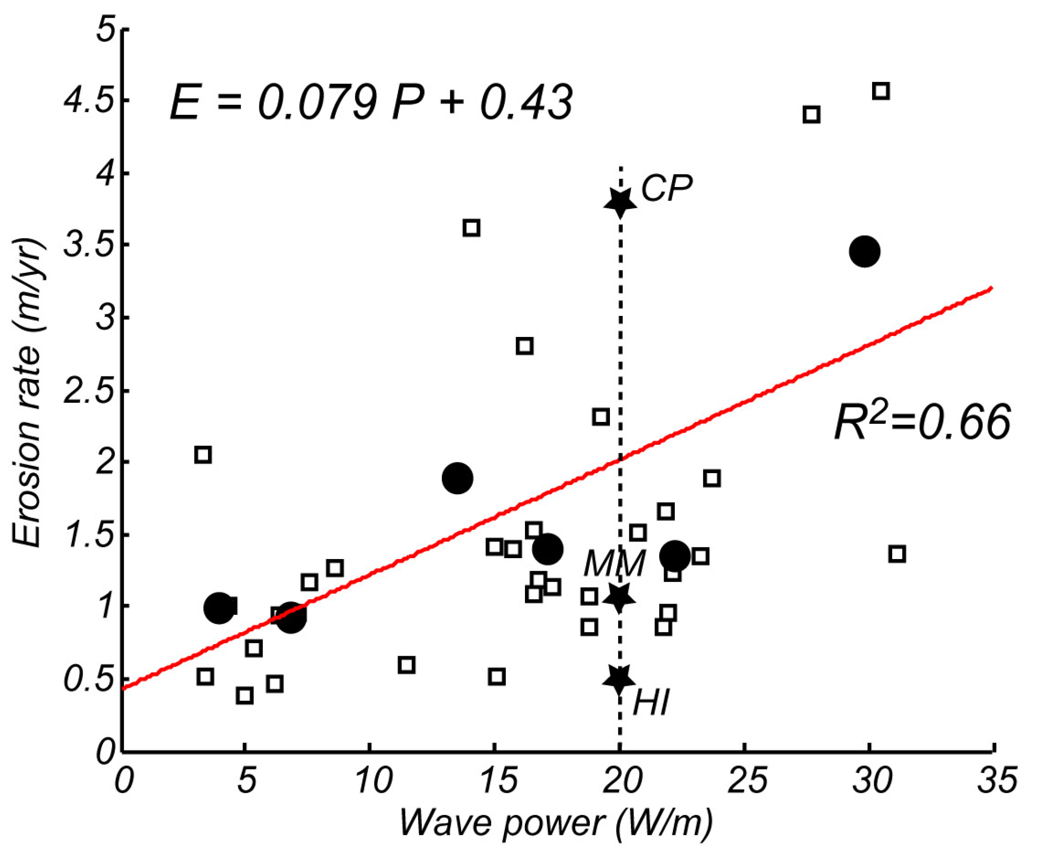
The slope of the relation, and therefore the rate of erosion, likely depends on soil type, water elevation, and possibly other factors, such as vegetation and macrofauna. Leonardi and Fagherazzi [
5,
6] used the formulation:
where
α, and
β are constant coefficients [
28],
P is the wave power, and
H is the wave height. The subscript
i refers to salt marsh portions which are homogeneous in terms of marsh platform erosional resistance,
Ei is the erosion rate of the above mentioned homogeneous marsh portions,
Hci is the critical height for marsh boundary stability and can be calculated from soil shear strength values [
32]. This formulation has been found in agreement with long-term field data of marsh boundary erosion and soil shear strength at five sites along the United States Atlantic Coast. The formula allows taking into account variability in erosional resistance along the marsh platform due to biological and ecological processes, and is suitable to reproduce the frequency-magnitude distribution of erosion events, as well as complex marsh boundary morphological features [
5,
6]. The formulation is such that when wave forces are very high (
H >>
Hci), the exponential goes to one, and every marsh portion looks the same in front of the main external driver with the same erosion probability. On the contrary, when wave energy is very low (
H ≤ Hci), variability in erosional resistance is more important and weakest elements are easily eroded. According to this formulation, different values of marsh boundary sinuosity have been related to different wind wave exposures. Specifically, high wave-power values cause more uniform marsh boundary profiles. On the contrary, salt marshes exposed to low wave-power conditions, and slowly eroding marshes, have been found to display rougher marsh boundary profiles [
5,
6]. Moreover, while rapidly eroding salt marshes display a Gaussian frequency-magnitude distribution of erosion events, slowly eroding salt marshes have been found to be characterized by long tailed frequency-magnitude distribution with a large number of small erosion events and a few number of unpredictable and high magnitude episodes.
Salt marsh lateral retreat has been also related to wave thrust values at the marsh boundary [
26]. Wave thrust is defined as the integral along the vertical of the dynamic pressure of waves. It has been shown that wave thrust is highly dependent on tidal levels. Specifically, wave thrust increases with tidal elevations until the marsh is submerged, and at that point the wave thrust starts to rapidly decrease. Decreasing wave thrust is attributed to wave breaking and wave energy dissipation on the vegetated marsh platform.
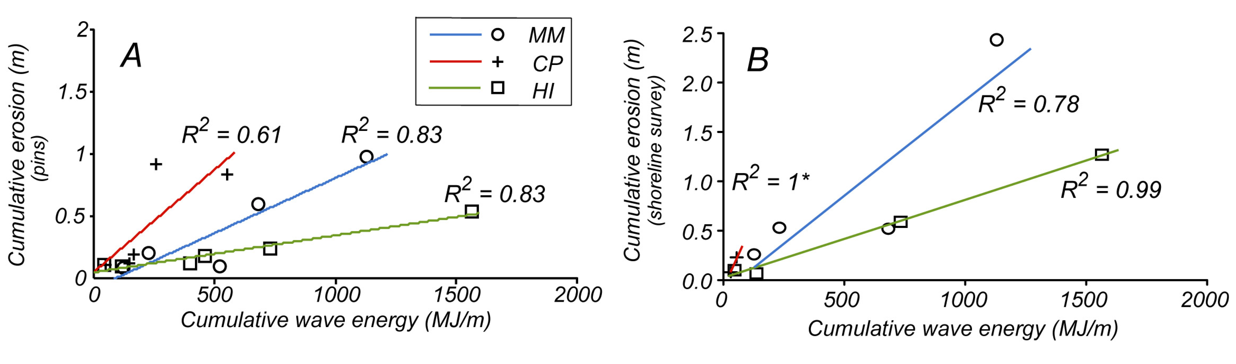
Herein, we will further test the relationship between wind-wave exposure and salt-marsh lateral retreat. We correlate salt-marsh lateral retreat with both wave power and wave thrust values at corresponding locations. The existence of a relationship between wave forcing and salt-marsh lateral retreat has been verified for cumulative values of the mentioned variables, as well as for their annual averages. Cumulative values are cumulative erosion (m), and cumulative wave energy (MJ/m) relative to time spans between field surveys.
3. Study Area
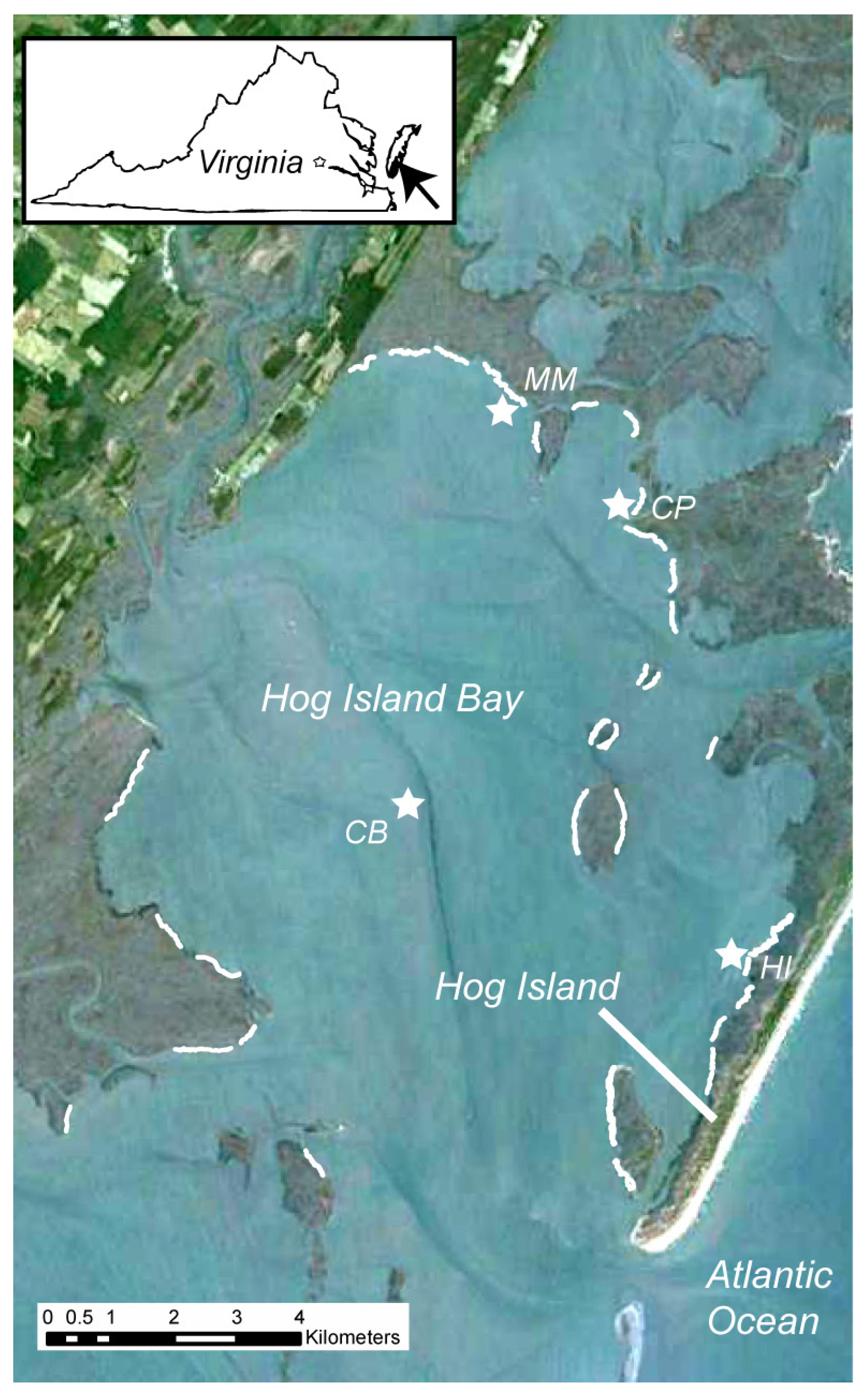
The study area is part of the Virginia Coast Reserve Long-Term Ecological Research network (VCR-LTER), which comprises a 110-km dynamic system of barrier islands, shallow lagoons, and salt marshes separated by deep tidal inlets. Our research is focused within Hog Island Bay, a coastal barrier lagoon located along the Atlantic side of the southern Delmarva Peninsula (
Figure 2). The lagoon is roughly 150 km
2 of predominately open water and is characterized by intertidal and subtidal basins with mainland fringe-marshes to the west, backbarrier-fringe marshes to the east, and platform marshes to the north and south. Vegetation on the salt marshes is dominated by short-form
Spartina alterniflora with an average stem height of 30 cm. The majority of the marshes have a prominent scarp at their seaward edges, which are typically 1.0–1.5 m above the elevations of the adjacent tidal flats.
The average water depth for most of the lagoon is about 2 m with respect to mean low water (MLW) and rarely exceeds 3 m [
33]. Semidiurnal tides have a mean tidal range of about 1.2 m (NOAA station 8631044). Water exchange occurs primarily through the Great Machipongo Inlet, maintained by a submerged deep thalweg that spans the lagoon floor to the mainland [
33].
Local weather patterns are dominated by the Bermuda high-pressure system [
34], giving rise to mostly calm conditions in the lagoon during the summer months, and the passage of cold fronts and Northeasters during winter [
35], which are largely responsible for storm conditions, in addition to occasional hurricanes. The area is highly influenced by storm disturbances, receiving an average of 20 extratropical storms per year [
36]. The distribution of wind speed and direction measured from 1993 to 1996 reveals that the most frequent wind directions originate between 180°–210° N and 330°–60° N with wind speeds usually less than 12 m/s [
29].
4. Methods
4.1. Field Survey of Marsh Shoreline Erosion
Three marsh sites (Matulakin Marsh, MM, Chimney Pole, CP, and Hog Island, HI) were selected in order to encompass different shoreline positions and orientations (white stars in
Figure 2). Retreat rates and morphology of the marsh shorelines were monitored through repeated surveys over a time span of three years from August 2007 to April 2010 (
Figure 3). Shoreline positions were measured using a Topcon laser-surveying total station. The time-spans between successive surveys are the following: 29 days, 6 May 2008 to 6 June 2008; 77 days, 6 June 2008 to 21 August 2008; 202 days, 21 August 2008 to 11 March 2009; 397 days, 11 March 2009 to 13 April 2010.
Figure 2.
Marshes in Hog Island Bay, part of the Virginia Coast Reserve, Virginia, USA. HI is Hog Island Marsh; CP is Chimney Pole Marsh, MM is Matulakin Marsh. Central Bay (CB) is the position where a wave gauge was deployed. White segments indicate marsh boundaries where erosion rates were measured with aerial images.
At each site, direct measurements of edge erosion were also made by using 6–7 erosion pins inserted horizontally into the marsh scarp. Due to the exploratory nature of field observations at the beginning of this research, the start times differ somewhat between sites. The total durations of erosion pin measurements at each site are as follows: MM (824 days, 9 January 2008 to 13 April 2010), CP (959 days, 28 August 2007 to 13 April 2010), HI (959 days, 28 August 2007 to 13 April 2010). Pins were reset after each measurement unless eroded out, in which case they were replaced.
Shoreline surveys yielded three pieces of information: (1) estimation of erosion rates along the length of the boundary; (2) characterization of shoreline morphology changes; and (3) computation of the frequency-magnitude distribution of erosion events and shoreline sinuosity to be related to wind wave exposure.
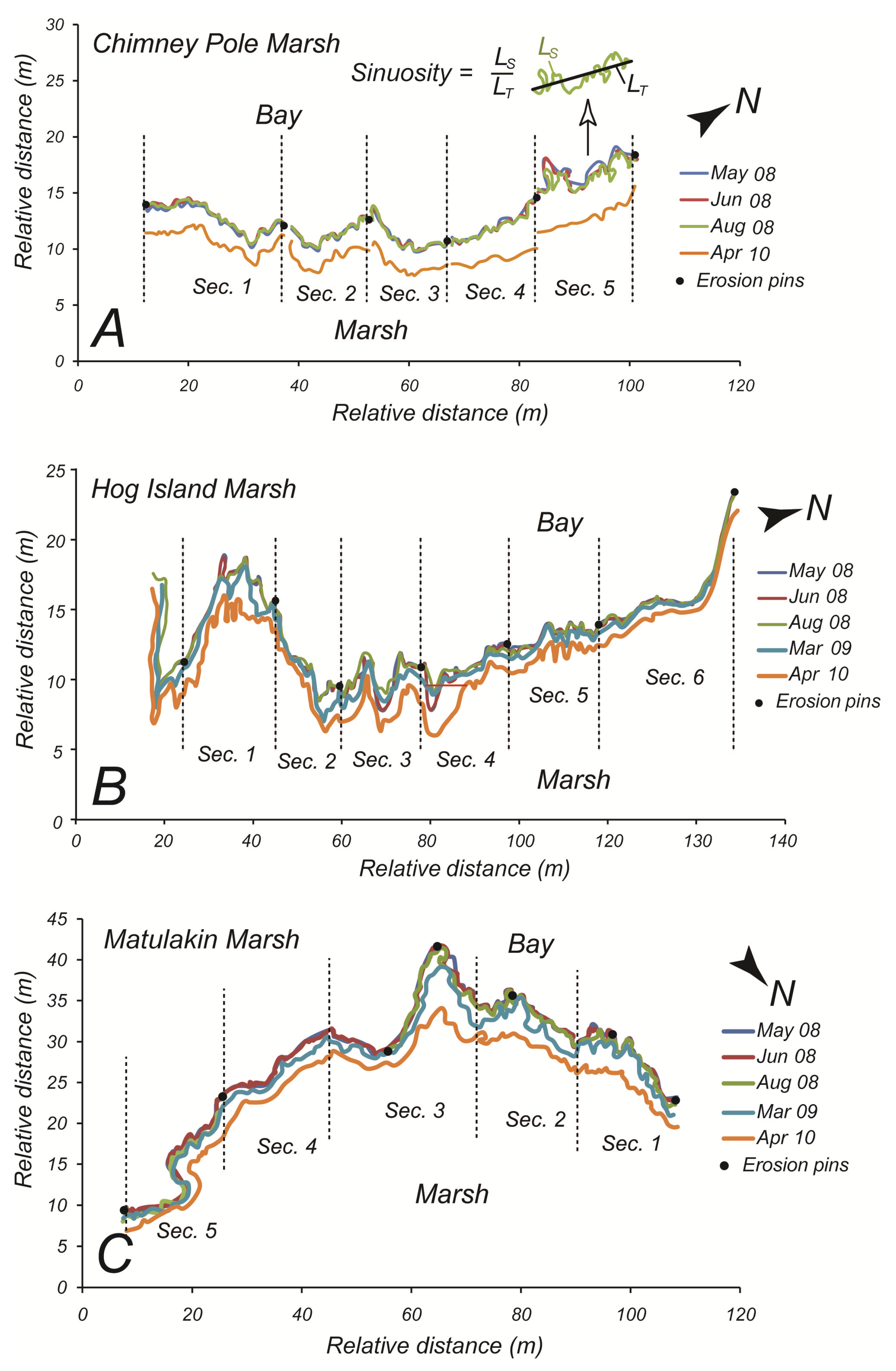
Figure 3.
High resolution surveys of marsh boundaries in Hog Island Bay between 2008 and 2010. (A) Chimney Pole Marsh; (B) Hog Island Marsh; (C) Matulakin Marsh. The vertical scale is distorted to better appreciate variations in boundary sinuosity. An example of boundary sinuosity calculation is reported in (A).
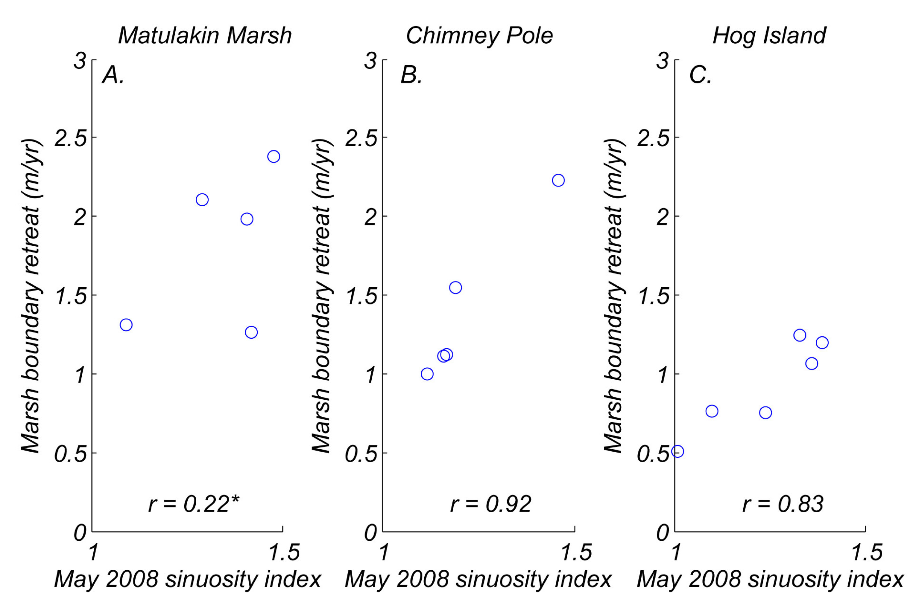
Marsh boundary sinuosity for the three sites has been calculated at two different scales: at the scale of the entire boundary length (order of hundreds of meters), and at a smaller scale (order of tens of meters). We maintain that at the scale of the entire marsh boundary length, variability in erosional resistance is present and there are thus stretches of marsh boundary that are more susceptible to erosion than others. This is due to the variety of biological and ecological mechanisms acting along marsh boundaries. On the contrary, we assume that at smaller scale (tens of meters), corresponding stretches of shoreline are relatively uniform in terms of erosional resistance, while also being sufficiently long to allow reasonable sinuosity calculations.
When calculating the marsh boundary sinuosity at a smaller scale our goal is to separate the influence of variability in erosional resistance along the marsh boundary [
5,
6] from the influence of wind waves on marsh boundary sinuosity, and focus on the latter. Sinuosity values were calculated as the ratio between boundary length and the length of the straight line between the two marsh boundary end points (
Figure 3A). Comparison in time between the same stretches of shoreline (
Figure 3) was used to evaluate the erosion rate between measuring periods.
Measurements of marsh boundary retreat with erosion pins and boundary surveys have limitations which need to be taken into account. For example, erosion pin measurements only provide few data points as representative of the entire marsh boundary. Regarding the surveys, the edge of the marsh scarp was not always well defined and it was assumed that the vegetation front would demarcate the boundary (we thus followed the definition of marsh as vegetated surface). In this situation, erosion rates determined from surveys would sometimes overestimate the total volume of sediment removed, since the root mat of the vegetation can recede faster than the scarp itself at some locations.
4.2. Estimating Marsh Erosion from Aerial Photographs
Field measurements of marsh shoreline erosion have limitations connected to the fact that they are only feasible for relatively small spatial extents. To overcome this limitation, we further determined erosion rates at 33 locations around the lagoon using two ortho-images from 2002 and 2009 (
Figure 2, continuous white lines). The aerial image from 2002 is part of the Virginia Geographic Information Network (VGIN), is available for public download by the GIS Center at Radford University, and was produced by VARGIS LLC of Herndon, Virginia. The acquisition date over the study area was 19 January 2002, the image was developed at a resolution of 2 m (1:400), and referenced in Virginia (south) state plane coordinate system.
The digital orthophotograph from 2009 is part of the National Agriculture Imagery Program (NAIP) and is available through the Aerial Photography Field Office (APFO) of the USDA Farm Service Agency. These images were acquired at a resolution of 1 m (1:200) and were rectified within ±6 m to true ground before being published. The images were then referenced to UTM zone 18 coordinate system using the North American Datum of 1983 (NAD 83). The 2002 and 2009 aerial images for the region were added into ArcMap using APFO’s ArcGIS server, and were then georeferenced in ArcMap to the 2009 imagery.
4.3. Modeling Wind Waves and Determination of Wave Power
4.3.1. Wave Hindcasting
Wave regime in the VCR lagoons was hindcasted using the spectral wave model SWAN, which solves the transport equations for wave action density, and accounts for shoaling, refraction, wind waves generation, wave breaking, bottom dissipation, and non-linear wave interactions [
37,
38,
39]. A rectangular grid with 200 by 300 cells with a resolution of 150 m was used to represent the lagoons’ bathymetry (
Figure 4). For the wind term, the exponential wind input of Yan [
40] and the linear growth of Cavaleri and Malanotte-Rizzoli [
41] were used in the simulations. The process of whitecapping was represented by the van der Westhuysen
et al. [
42] formulation, based on the azimuthal-integrated spectral saturation. Depth induced breaking was described by the physically-based formulation of van der Westhuysen
et al. [
43], which relates the nonlinearity of breaking waves in shallow water to wave asymmetry.
A total of 900 simulations were performed, combining 15 water levels (every 0.2 m, from −0.8 m below M.S.L. to 2 m above M.S.L.), 5 wind speeds (5, 10, 15, 20, 25 m/s) and 12 wind directions (every 30°). In each simulation, water level, wind speed, and direction were imposed uniform throughout the domain. Simulations were performed in steady conditions,
i.e., the wave field was in local equilibrium with the energy sink-source terms. We also assumed that the wave direction is always corresponding to the wind direction, given the small fetch and the absence of waves propagating from offshore. For each simulation, a single value of the significant wave height,
H, and peak wave period,
T, were extracted at each marsh boundary position,
i. We therefore obtained two discrete functional relationships, relating
H and
T to the water level,
y, wind speed,
U, and direction,
α, at each marsh boundary position:
The relationship between Hi and Ti was made continuous through a linear interpolation.
Water-level measurements were retrieved from the Wachapreague NOAA station (ID 8631044). Lawson
et al. [
44] modeled waves in Hog Island Bay with SWAN using the wind speed from the Kiptopeke NOAA station (ID KPTV2), whose record started in 2005. In order to base our results on a longer time series, we instead use the wind speed and direction data from the NOAA station CHLV2-Chesapeake Light, whose record started in 1984. This station is located outside the lagoons, about 10 km from the coastline, and likely overestimates the wind speed within the lagoons.
After comparison, we determined that the wind speed from the Chesapeake Light station is 20% higher than the wind speed at the Kiptopeke station when data are available at both stations, while the wind direction is similar. We hence obtain a time series of hourly water level, wind speed, and direction from 1 April 2002 to 14 April 2010 by reducing of 20% the entire time series of wind speed at the Chesapeake Light. 22% of the time series had missing data on either water level or wind conditions. For each site, the time series Hi and Ti were reconstructed using Equation (7).
4.3.2. Model Validation
The results were validated using two wave events: Period 1, from 31 January to 5 February 2009 and Period 2, from 1 March to 2 March 2009, using wave data collected in the field and reported in Mariotti
et al. [
29]. The performance of SWAN in reproducing wave height and wave period is evaluated using the Root Mean Square Error and the Model Efficiency. The latter measures the ratio of the model error to variability in observational data, and its performance levels are categorized as: >0.65 excellent; 0.65–0.5 very good; 0.5–0.2 good; <0.2 poor [
45]. The performance of SWAN is analogous to the numerical model used in Mariotti
et al. [
29]: the Root Mean Square Error in the wave height is around 10 cm, while the Model Efficiency for the wave height is between −2.1 and 0.4 (
Figure 5).
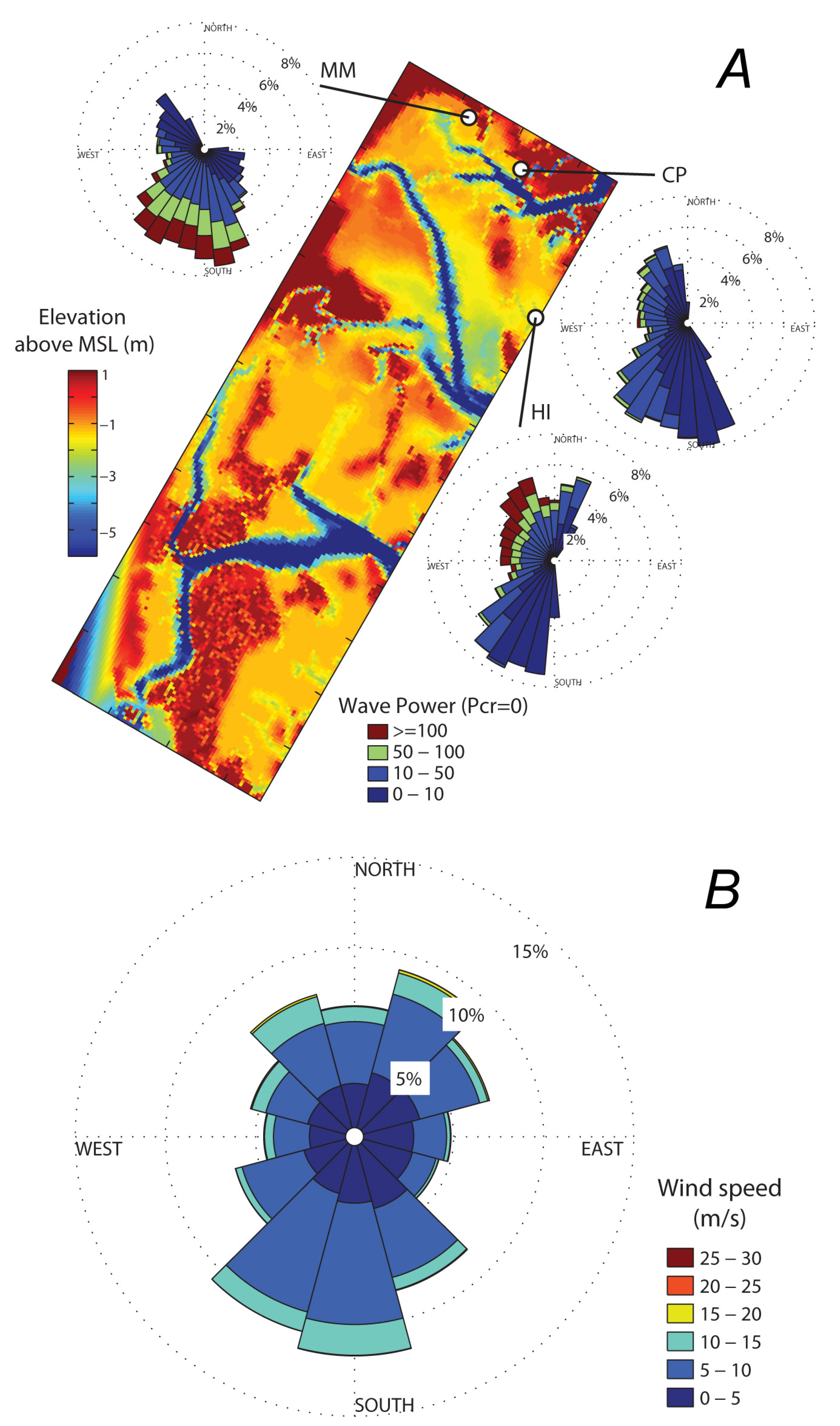
Figure 4.
(A) Digital elevation model of Hog Island Bay used to hindcast wave height and wave period with the SWAN model. The distribution of wave power (W/m) and directions from the model output is shown for each study location; (B) distribution of wind speed (m/s) and directions used to force the model.
Figure 5.
Model simulations of significant wave height and wave period validated against measured data for the three study sites. Wind data from NOAA Wachapreague station 8631044; (A) wind speed and (B) wind direction for period 1. Wave period for (C) Matulakin Marsh; (E) Hog Island Marsh; (G) Chimney Pole; (I) Central Bay. Wave height for (D) Matulakin Marsh; (F) Hog Island Marsh; (H) Chimney Pole; (L) Central Bay. (M) wind speed and (N) wind direction for period 2; (O) Wave period for Central Bay; (P) wave height for Central Bay.
4.3.3. Proxy for Salt Marsh Boundary Erosion
Three proxies for marsh boundary erosion were considered: wave height (m) at the marsh boundary, wave power (W/m) incident to the marsh boundary [
28] and the wave thrust (kN/m) acting on the marsh boundary [
26]. In analogy to erosion of a horizontal bed of sediment (
i.e., the Shields parameter), we hypothesize the existence of a threshold in wave energy below which erosion is zero. Wave erosion thresholds were designed to address the effects on erosion due to differences in wave energy magnitude
versus duration. The goal of this task is to determine whether erosion is predominately a result of low-energy, frequent events, or high-energy infrequent events. We attempt to address this question by computing the wave power using different erosion thresholds and comparing the correlation between results without the threshold.
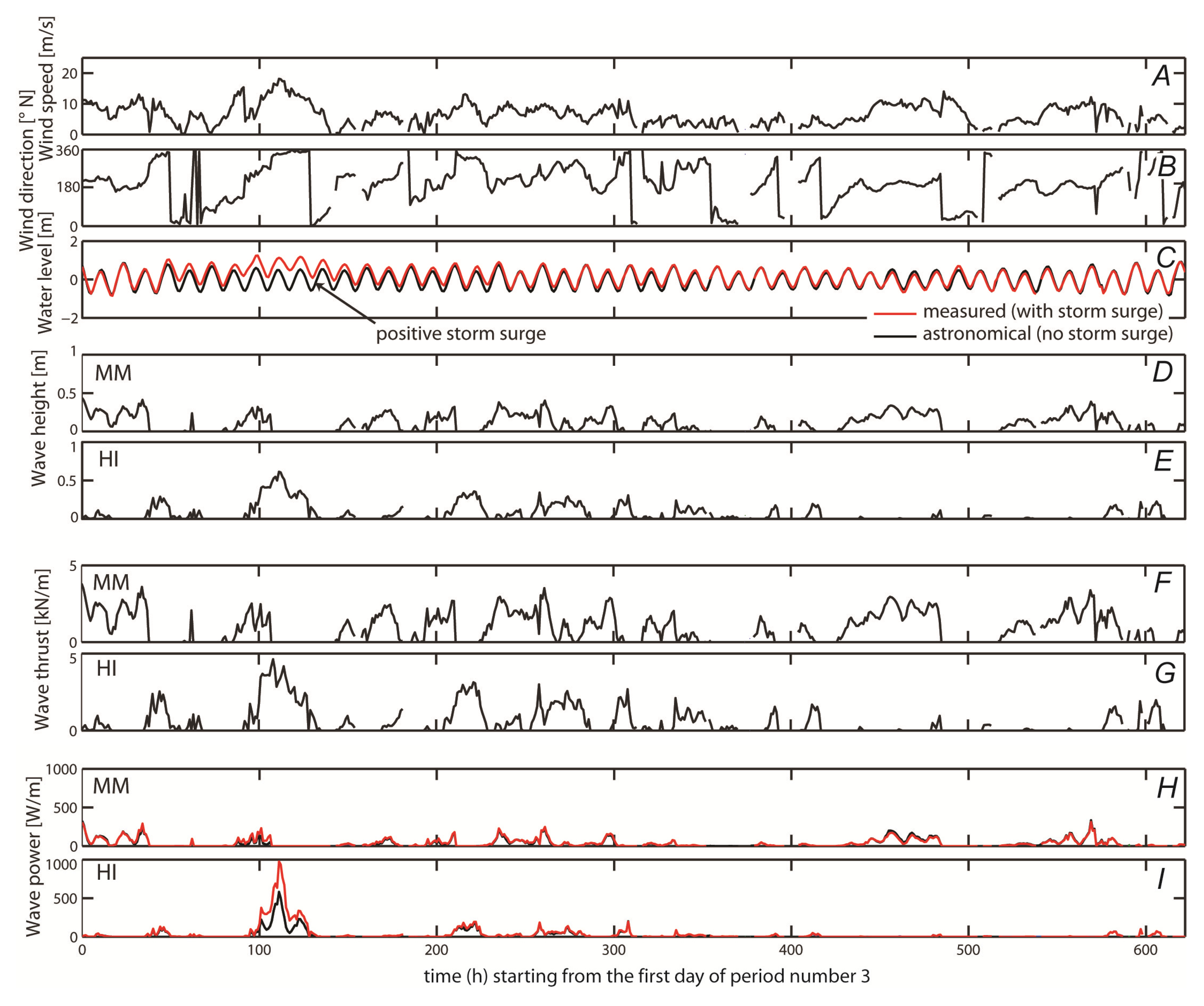
Figure 6.
Sample time series reconstruction (21 August 2008 to 13 April 2010) of modeled wave height, wave thrust, and wave power using measured (with storm surge) and predicted (no storm surge) water levels for two study sites. The full reconstruction for data analysis spans from 1 April 2002 to 19 April 2010 for all three study sites. Note peak wave power at the HI location (t = 110 h) due to the storm surge, which is double the wave power without storm surge.
The excess incident wave power (W/m) was computed as:
where
cg is the group velocity,
E the wave energy (J/m
2), and
θ the angle between the wave direction and the normal to the marsh boundary.
Pcr represents a threshold in marsh boundary erosion [
29,
30], introduced in analogy with the threshold in bottom sediment erosion.
The wave thrust was computed using the results of Tonelli
et al. [
26]. The maximum wave thrust (kN/m) for the case of a vertical bank is approximated as:
where
h is the water depth in front of the marsh boundary and
hb is the height of the marsh platform. The dependence on the period is neglected. Different from wave power, the use of the wave thrust takes into account the effect of reduced marsh boundary erosion when the water level is higher than the marsh top.
Using the time series
Hi,
Ti and
y, we reconstructed the times series
Pi and
Wi, using both the measured and the predicted water levels. A sample from the whole time series is given in
Figure 6. This example clearly shows the effect of storm surges: the maximum wave power (
Figure 6,
t = 110 h) at the HI site computed by considering the measured water level is almost double the maximum wave power computed with the predicted (astronomical) water level.
7. Conclusions
High-resolution measurements of lateral salt marsh erosion at the sub-meter scale were conducted along the boundary between marshes and Hog Island Bay at the Virginia Coast Reserve, USA. These measurements, together with erosion rates estimated from aerial photographs for a seven years period, complemented and expanded a long-term dataset of marsh erosion at this location [
7]. Erosion rates were compared to wind wave characteristics computed with the numerical model SWAN. We confirm the existence of a previously shown relationship between salt-marsh lateral retreat and wave forcing. According to our analysis, salt-marsh erosion is a process continuous in time. This is confirmed by the existence of significant relationships between cumulative wave energy and erosion over sub-periods, as well as between the averages of the same variables.
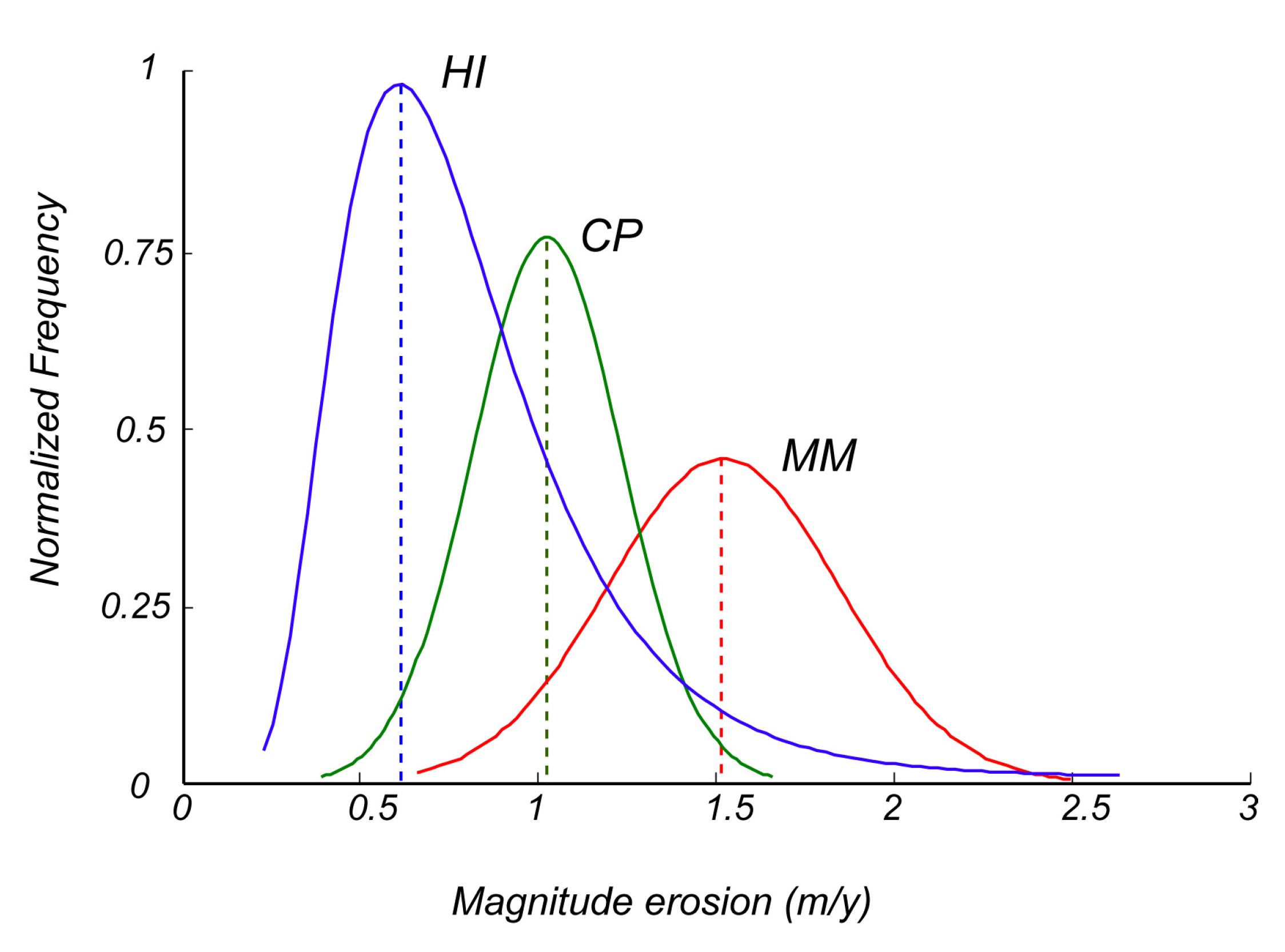
Salt-marsh boundary erosion is primarily a linear function of wave power, the rate of which averages about 1.3 m/year within Hog Island Bay, Virginia, USA. The primary mechanisms of marsh retreat are corrasion, block detachment, root-scalping, and formation of wave-gullies, which greatly depend on the tidal elevation during wave generation. At a given site, short-term erosion data (temporal scale of months) are very similar to medium-term erosion data (temporal scale of years) and to the long-term data (temporal scale of decades) reported in McLoughlin
et al. [
7]. However, erosion rates and their relationship to wave power considerably vary from site to site, possibly due to local morphological, sedimentological, and biological factors affecting the resistance of the marsh boundary. At the scale of tens of meters, we found a positive correlation between sinuosity and erosion rate due to positive feedbacks between the morphology of the marsh boundary and wave action, indicative of the formation of wave-cut gullies. However, at a larger scale this relationship is reversed and high sinuosity corresponds to slowly eroding salt marshes, while low sinuosity corresponds to rapidly eroding boundaries.
Marsh erosion is correlated to wave power and less related to wave height or wave thrust. The introduction of a threshold for wave power below which erosion is negligible does not increase in a significant way the correlation between wave power and erosion rate. Similarly, neglecting storm surges does not decrease the correlation between wave power and erosion rate. We therefore conclude that, at the level of approximation of our study, the inclusion in numerical models of a wave power threshold for erosion or the utilization of astronomic tidal elevations rather than measured water levels do not significantly affect the estimate of marsh erosion.


