
Wind Turbine Blade Life-Time Assessment Model for Preventive Planning of Operation and Maintenance


Abstract
:1. Introduction
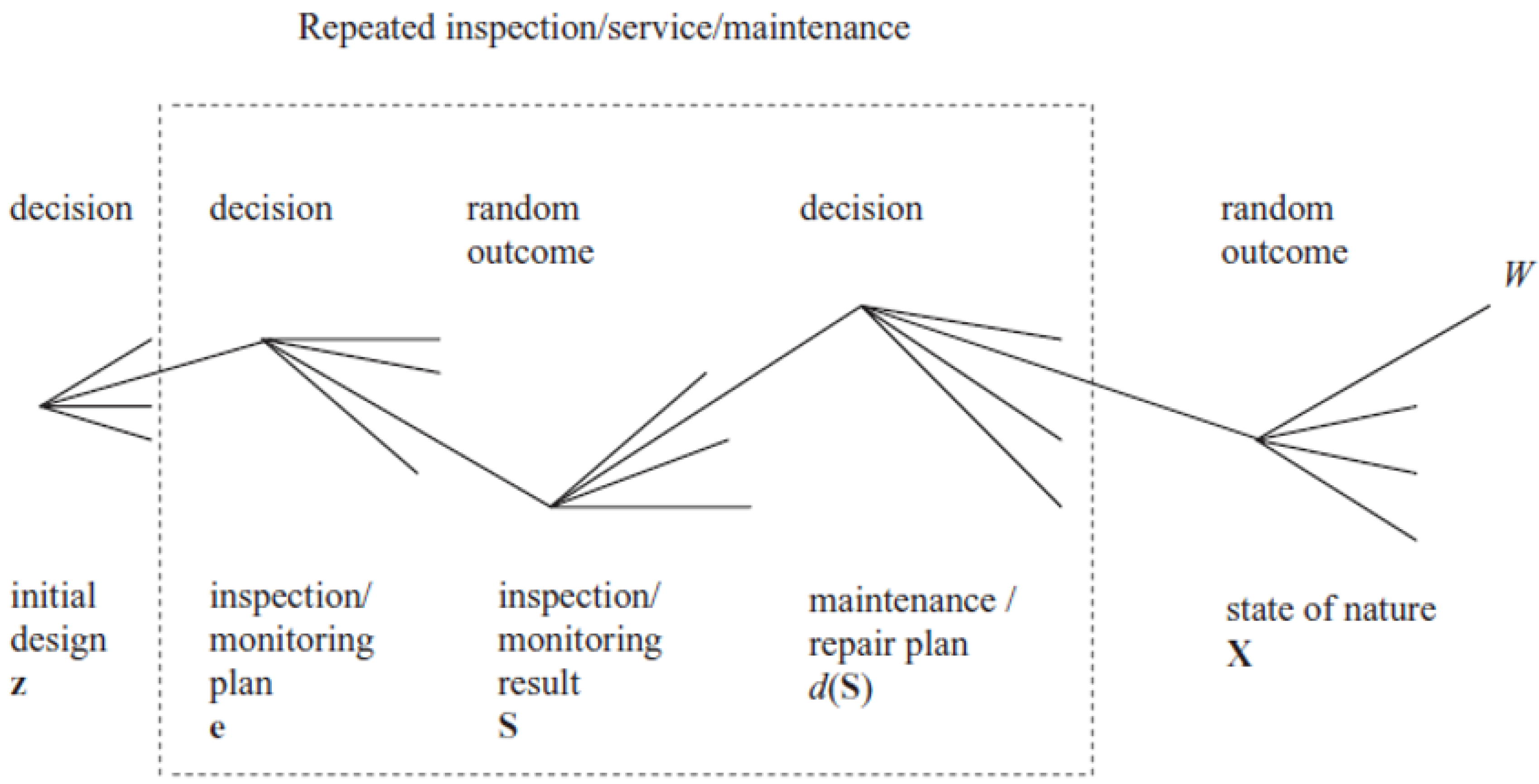
2. Optimal Maintenance and Inspection Planning
3. Model Description
3.1. Weather Conditions
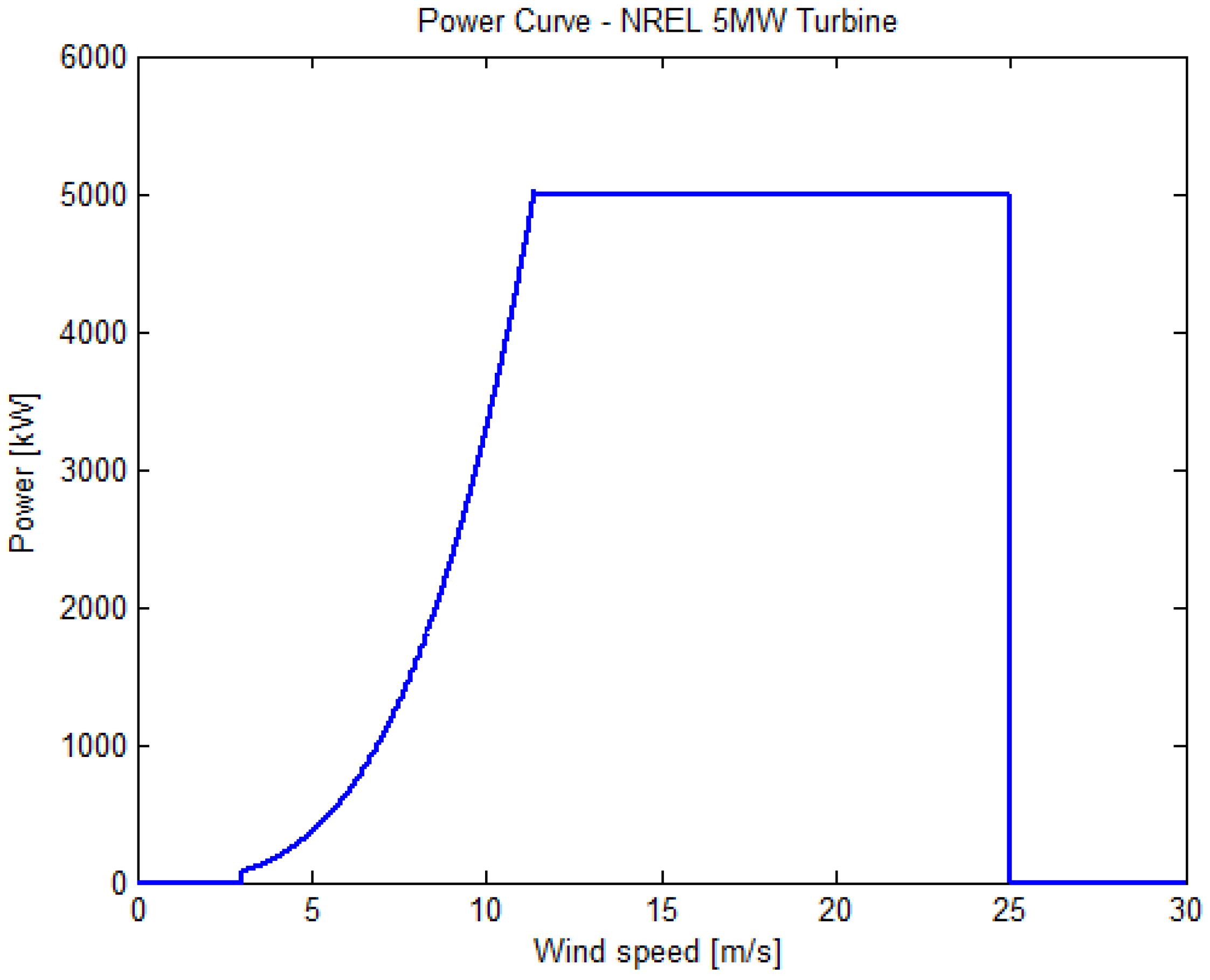
3.2. Power Production
3.3. Transport

| Symbol | Description | Value | Unit |
|---|---|---|---|
| Ulim | Wind limit | 12 | m/s |
| Hs,lim | Wave limit | 1.5 | m |
| Ttr | Transport | 8 | h |
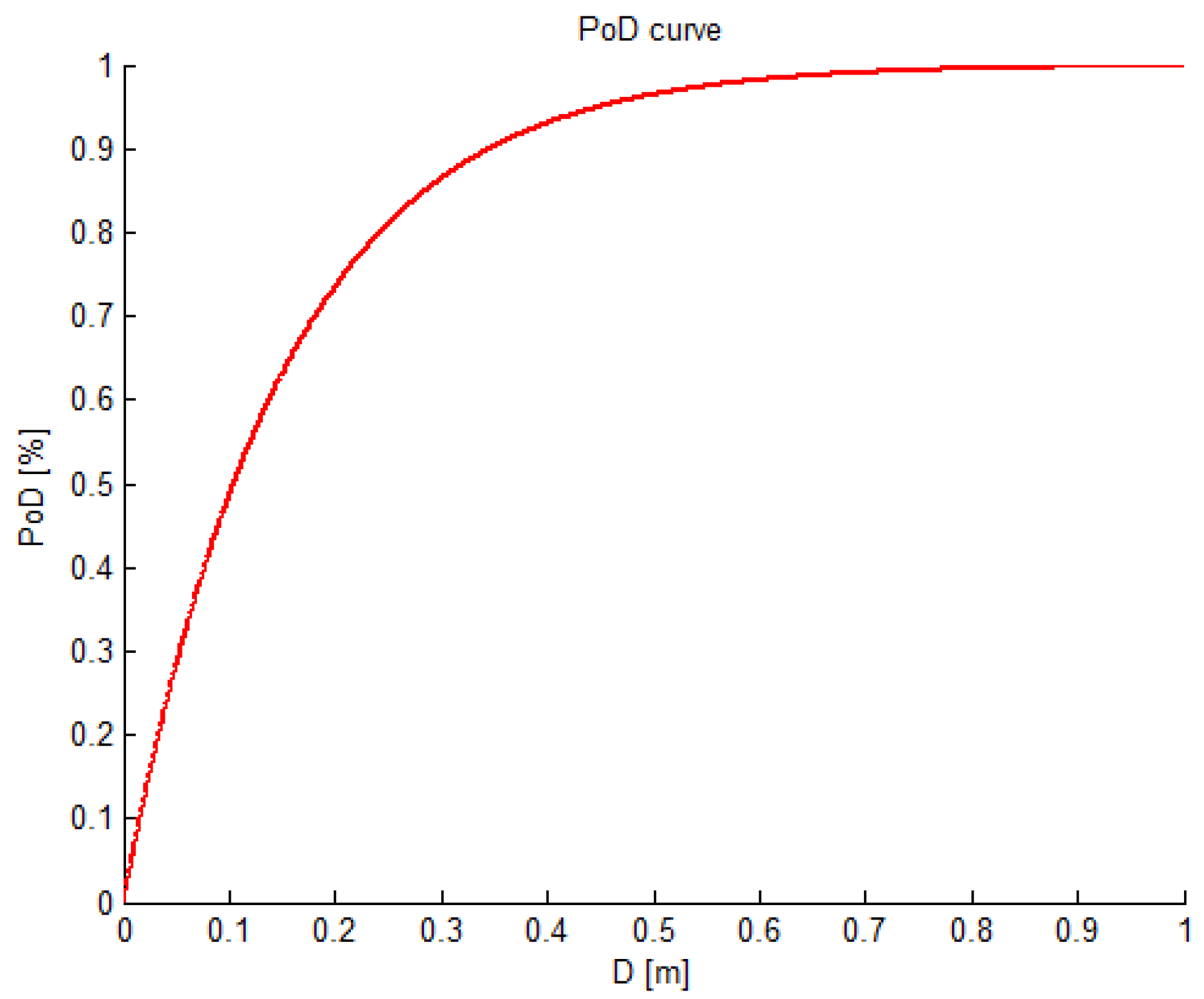
3.4. Inspections
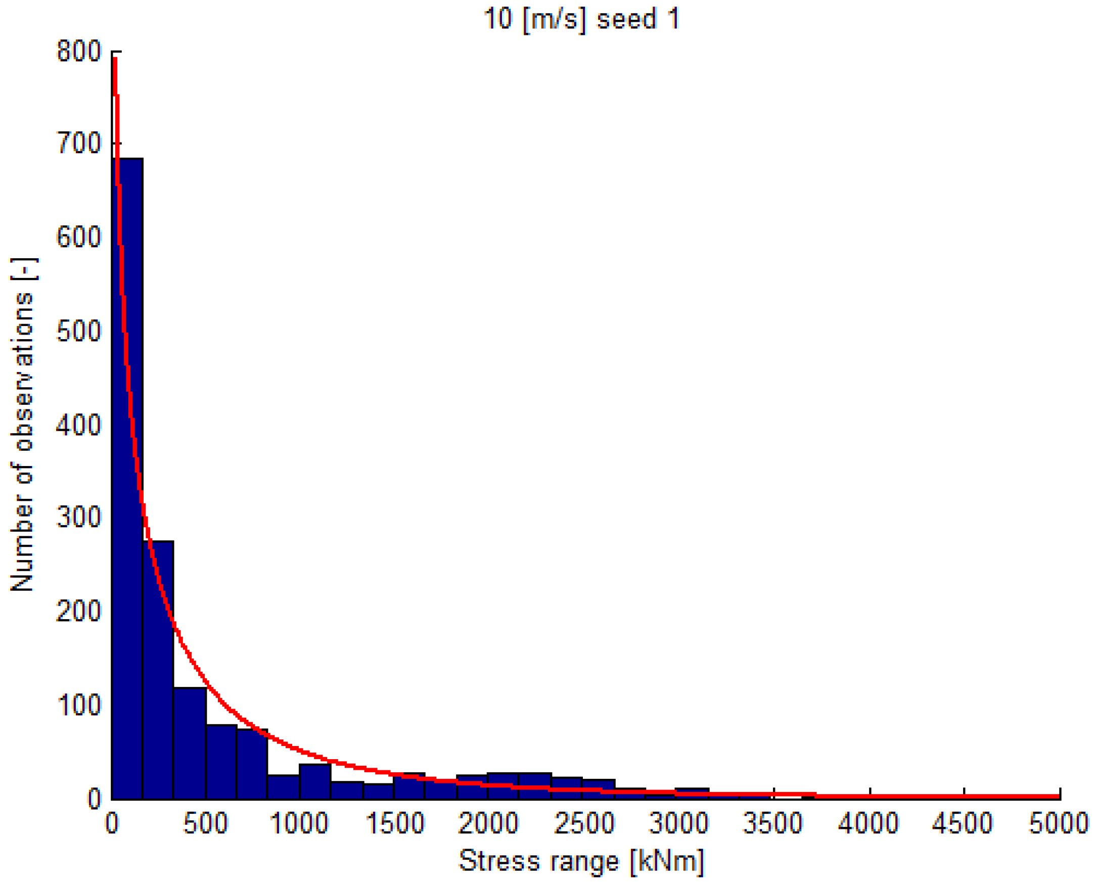
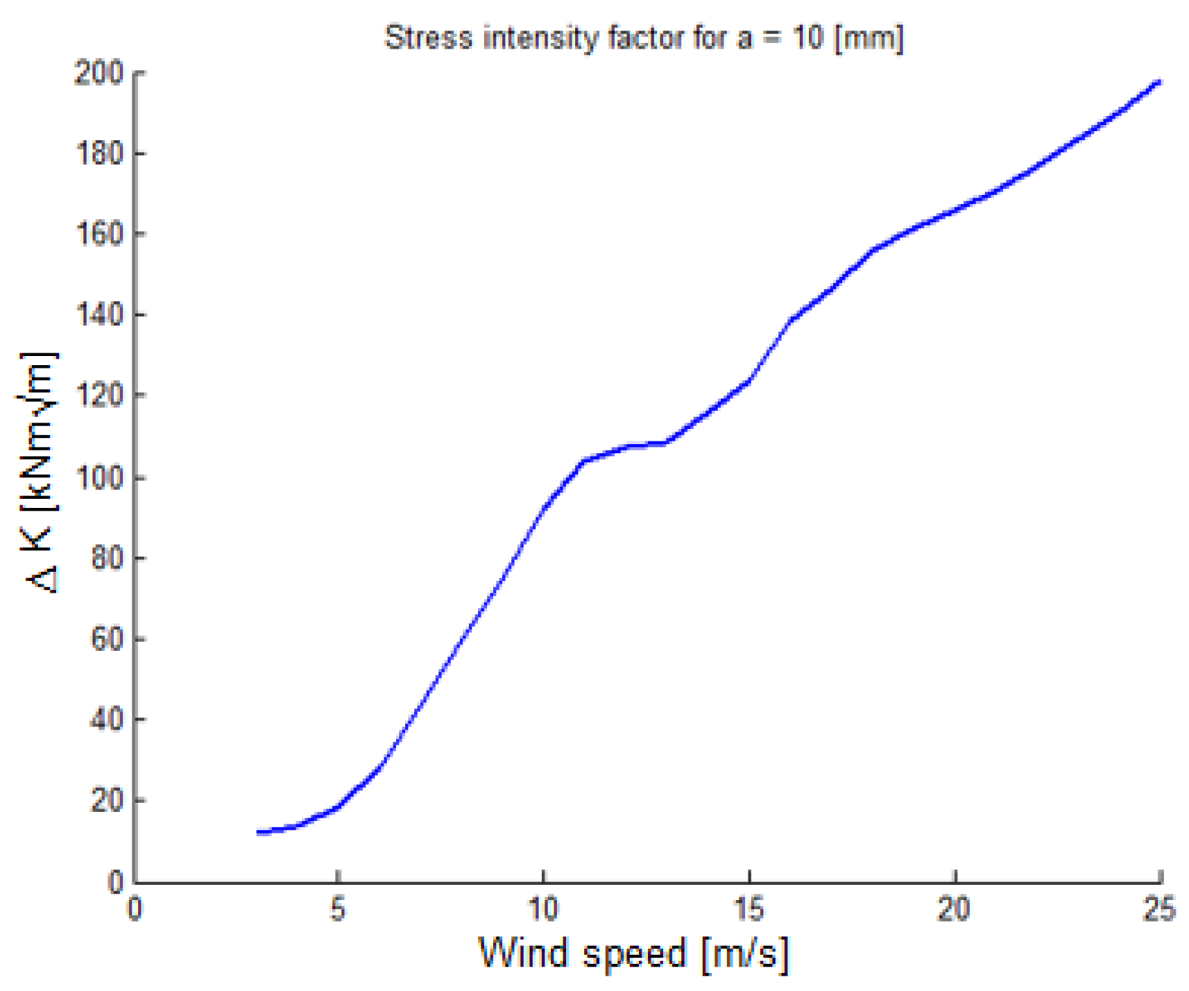
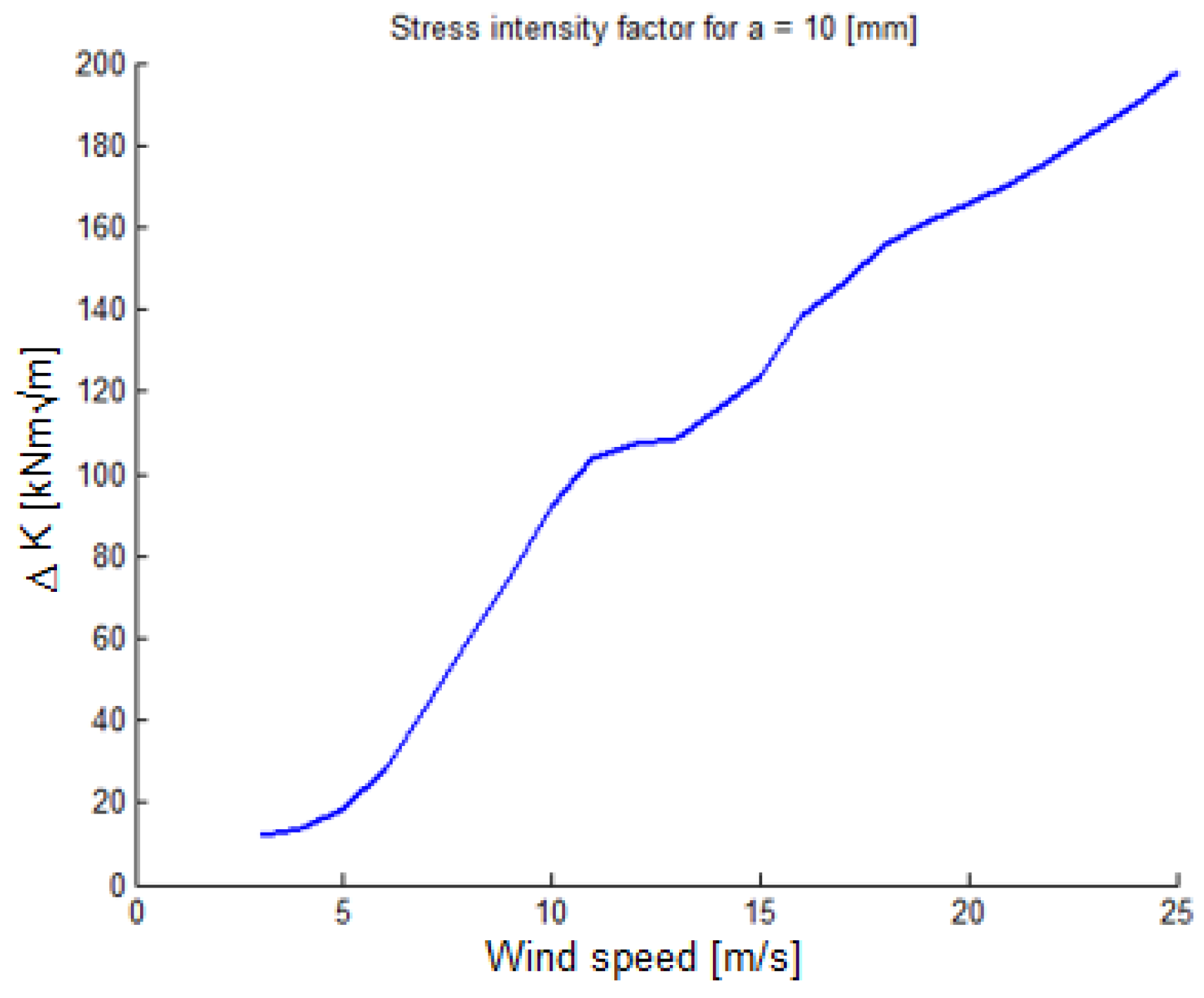
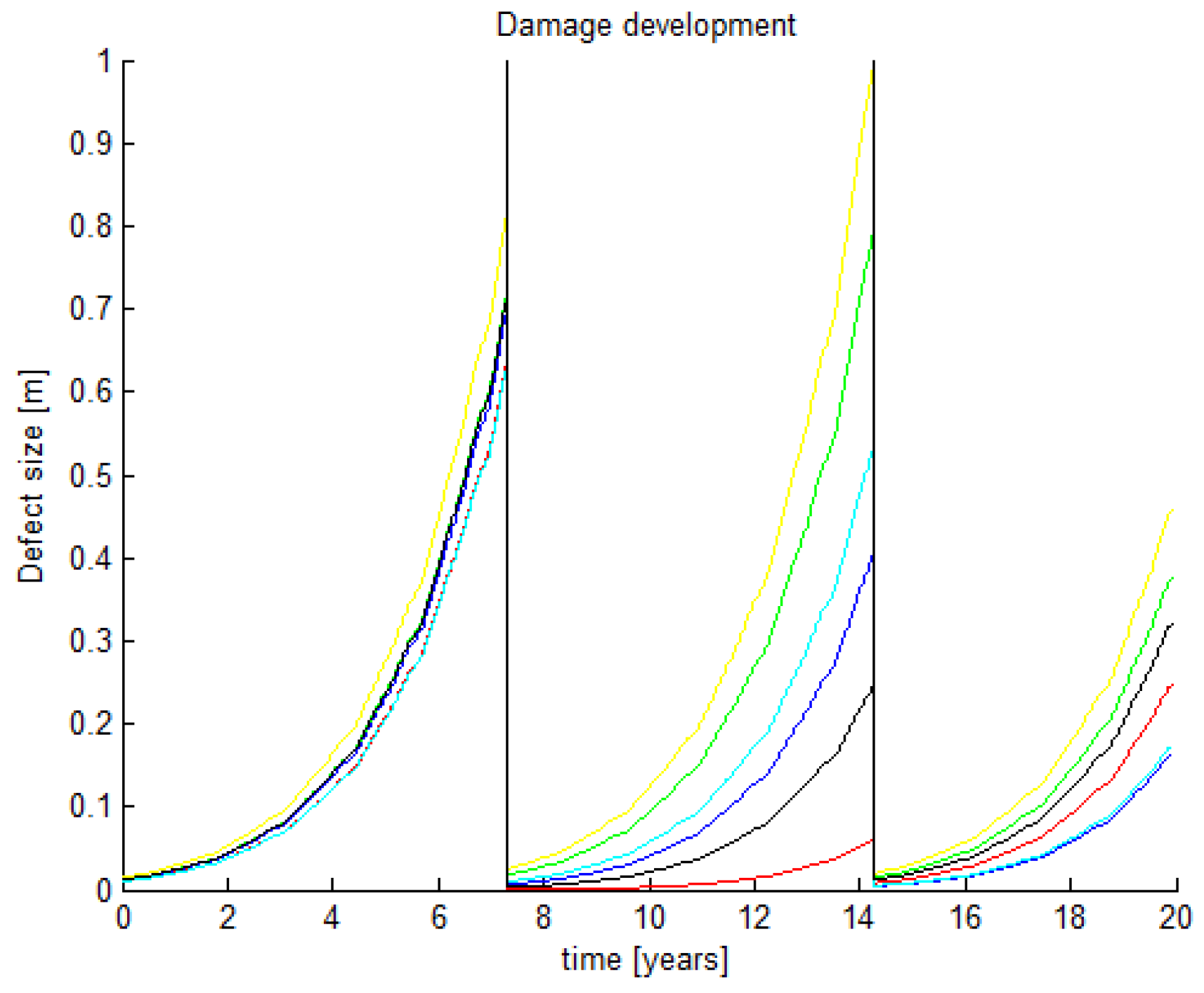
3.5. Damage Model
- crack initiation at the start of the blade’s life
- damage propagation during the blade’s lifetime
- failure is achieved when a crack length reaches afail
- da
- Increase in crack length
- ΔK
- Stress intensity factor
- Δt
- Time period
- A,m,λw
- Material parameters
- R
- Stress ratio
- Δs
- Load range
- a
- Crack length
- f(Δs|u,I)
- Density function of load cycles

3.6. Repair Model
| Preventive | 24 h |
| Corrective | 72 h |
3.7. Cost Model
| Activity | Symbol | Value | Unit |
|---|---|---|---|
| Energy cost | CL | 0.04 | €/kWh |
| Inspection | CIN | 2,500 | € |
| Preventive repair | CREP | 10,000 | € |
| Corrective repair | CF | 100,000 | € |
3.8. Stochastic Model
| Parmeter | Dist | Mean | COV | |
|---|---|---|---|---|
| ain | LN | 10 | 0.15 | mm |
| A | LN | 1.2−9 | 0.05 | |
| m | N | 1.8 | - | - |
| λw | N | 0.8 | 0.05 | - |
4. Results and Discussion
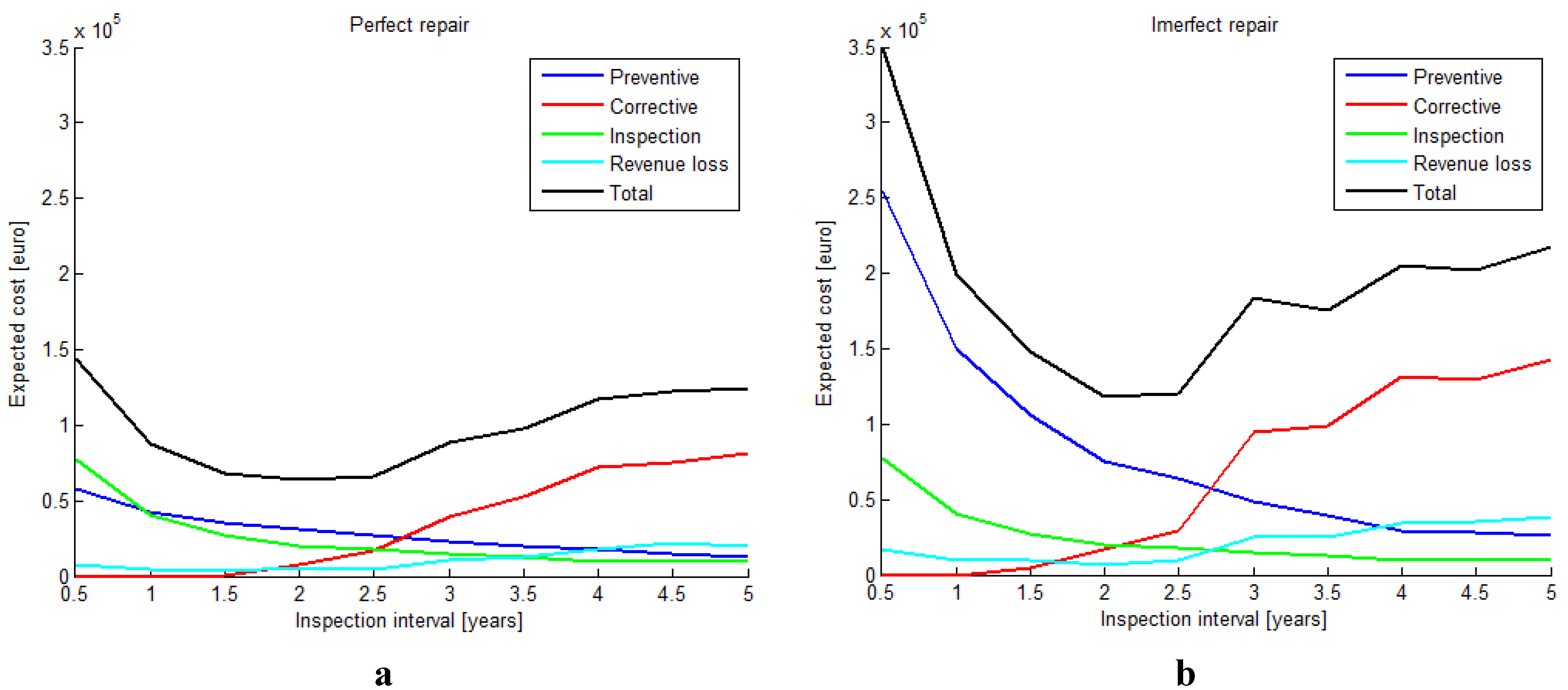
4.1. Inspection Interval

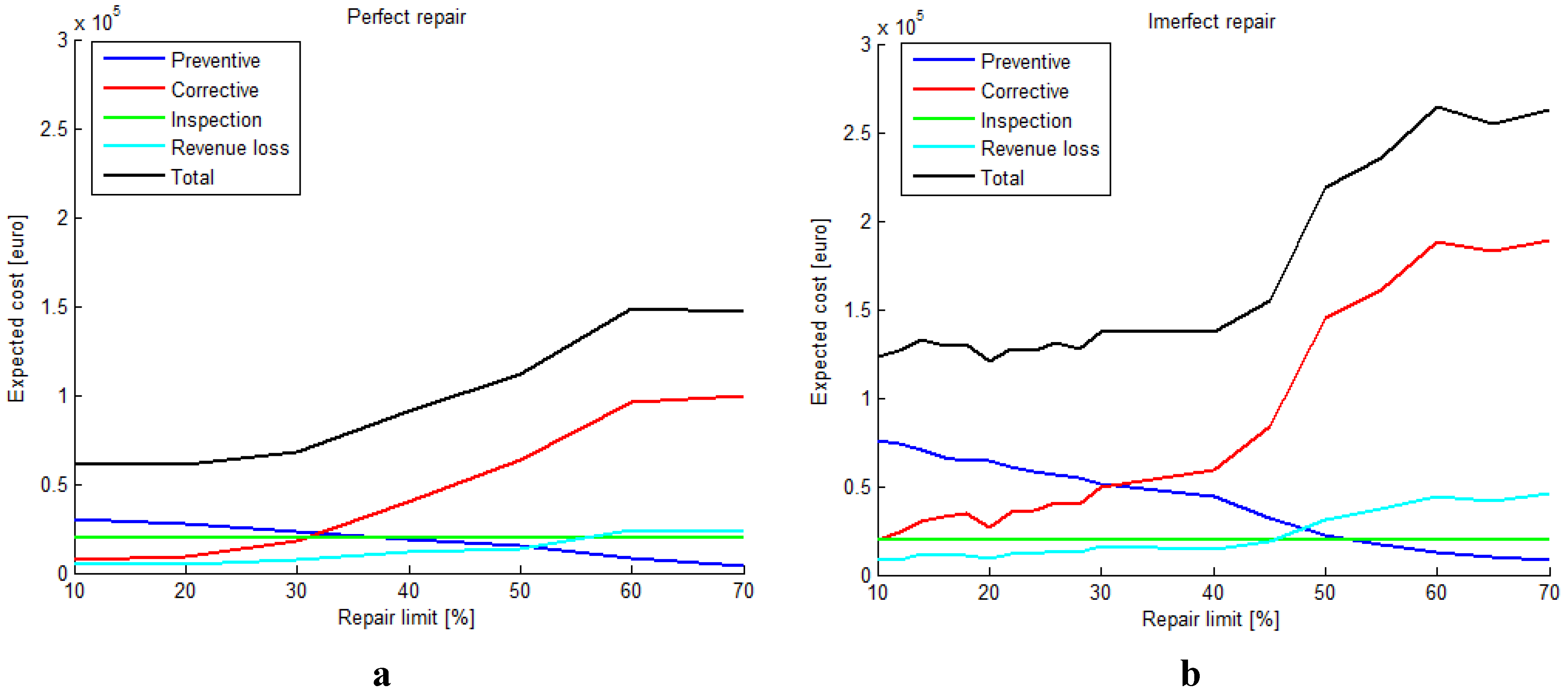
4.2. Repair Limit

5. Conclusions
Acknowledgments
Author Contributions
Conflicts of Interest
References
- Wouter, E.; Obdam, T.; Savenije, F. Current Developments in Wind—2009; Technical Report for Energy Research Centre of The Netherlands: Petten, The Netherlands, 2009. [Google Scholar]
- Chou, J.-S.; Tu, W-T. Failure analysis and risk management of a collapsed large wind turbine tower. Eng. Fail. Anal. 2011, 18, 295–313. [Google Scholar]
- Sørensen, J.D. Framework for risk-based planning of operation and maintenance for offshore wind turbines. Wind Energy 2009, 12, 493–506. [Google Scholar]
- Nielsen, J.J.; Sørensen, J.D. On risk-based operation and maintenance of offshore wind turbine components. Reliab. Eng. Syst. Saf. 2011, 96, 218–229. [Google Scholar]
- Jonkman, J.M.; Buhl, M.L., Jr. FAST User’s Guide; Technical Report for National Renewable Energy Laboratory: Golden, CO, USA, 2005. [Google Scholar]
- Yang, J.; Peng, C.; Xiao, J.; Zeng, J.; Xing, S.; Jin, J.; Deng, H. Structural investigation of composite wind turbine blade considering structural collapse in full-scale static tests. Compos. Struct. 2013, 97, 15–29. [Google Scholar] [CrossRef]
- Stephens, R.I.; Fatemi, A.; Stephens, R.R.; Fuchs, H.O. Metal Fatigue in Engineering; John Wiley & Sons: Hoboken, NJ, USA, 2001. [Google Scholar]
- Sørensen, J.D.; Frandsen, S.; Tarp-Johansen, N.J. Effective turbulence models and fatigue reliability in wind farms. Probab. Eng. Mech. 2008, 23, 531–538. [Google Scholar]
- Faulstich, S.; Hahn, P.; Tavner, P. Wind turbine downtime and its importance importance for offshore deployment. Wind Energy 2011, 14, 327–337. [Google Scholar] [CrossRef]
© 2015 by the authors; licensee MDPI, Basel, Switzerland. This article is an open access article distributed under the terms and conditions of the Creative Commons Attribution license ( http://creativecommons.org/licenses/by/4.0/).
Share and Cite
Florian, M.; Sørensen, J.D. Wind Turbine Blade Life-Time Assessment Model for Preventive Planning of Operation and Maintenance. J. Mar. Sci. Eng. 2015, 3, 1027-1040. https://doi.org/10.3390/jmse3031027
Florian M, Sørensen JD. Wind Turbine Blade Life-Time Assessment Model for Preventive Planning of Operation and Maintenance. Journal of Marine Science and Engineering. 2015; 3(3):1027-1040. https://doi.org/10.3390/jmse3031027
Chicago/Turabian StyleFlorian, Mihai, and John Dalsgaard Sørensen. 2015. "Wind Turbine Blade Life-Time Assessment Model for Preventive Planning of Operation and Maintenance" Journal of Marine Science and Engineering 3, no. 3: 1027-1040. https://doi.org/10.3390/jmse3031027
APA StyleFlorian, M., & Sørensen, J. D. (2015). Wind Turbine Blade Life-Time Assessment Model for Preventive Planning of Operation and Maintenance. Journal of Marine Science and Engineering, 3(3), 1027-1040. https://doi.org/10.3390/jmse3031027