Weak Calibration Cross-Fusion Framework for Multi-Modal 3D Object Detection on Unmanned Surface Vehicles

Abstract

The field of intelligent transportation on inland waterways is experiencing rapid growth, driven by the global pursuit of enhanced waterway safety, operational efficiency, and environmental sustainability. In real-world autonomous operation scenarios of unmanned surface vehicles (USVs), image-based 2D object detection methods are insufficient to meet the demands of 3D environmental modeling and accurate perception of dynamic objects. Existing 3D perception systems for USVs depend heavily on precise sensor calibration. However, projection offsets between point clouds and images—caused by water surface fluctuations and complex outdoor environments—hinder the practical deployment of these methods. To address these limitations, we propose a weak calibration multi-modal 3D object detection algorithm based on cross-view fusion, termed RCF-Free (Radar-Camera Fusion, Free from precise calibration). Inspired by autonomous driving solutions, we design a Triple-Path Cross-View Fusion module that achieves high-quality cross-view feature fusion without requiring accurate calibration parameters, while simultaneously detecting complete bird’s-eye view (BEV) bounding boxes. We further enhance the spatial layout comprehension of the visual branch through a Mobile Self-Attention Module (MAM) and effectively encode sparse point cloud features in BEV space using a dedicated BEV-Point feature encoder. Additionally, we reconstruct and introduce two water-related 3D object detection datasets, FloW-BEV and WaterScenes-BEV. Experimental results demonstrate that RCF-Free achieves $\mathrm{m}\mathrm{A}{\mathrm{P}}_{\mathrm{B}\mathrm{E}\mathrm{V}}50$ scores of 60.5% and 69.3% on the FloW-BEV and WaterScenes-BEV datasets, respectively, showing the effectiveness in water surface object detection. Moreover, on the DAIR-V2X-I dataset for autonomous driving scenarios, the model attains $\mathrm{m}\mathrm{A}{\mathrm{P}}_{3\mathrm{D}}50$ scores of 73.3%, 61.2%, and 61.2% across three task difficulty levels, illustrating strong cross-domain generalization capability.

1. Introduction

Intelligent transportation on inland waterways is an emerging field centered on the development of autonomous Unmanned Surface Vehicles (USVs) for applications in logistics, environmental monitoring, and safety assurance. Unlike open-sea environments, inland waters present unique perceptual challenges including confined channels, complex background clutter, and dynamic wave patterns induced by interactions with riverbanks and structures [1,2,3]. As a fundamental component of such systems, 3D object detection provides USVs with essential spatial information—including precise coordinates, orientation, and dimensions of objects—which is crucial for situational awareness and navigation decision-making [4,5]. However, 3D perception on water surfaces remains highly challenging due to factors such as water surface reflections, wave surges, variable illumination, and the inherent limitations of onboard sensors.

From a sensor perspective, cameras offer rich texture and color information at low cost but are susceptible to optical interference (e.g., lighting variations and reflections) and lack the capability for direct 3D environmental measurement. In contrast, LiDAR can provide dense, high-precision point clouds, but in complex inland water environments, it often fails to distinguish target objects from extensive background clutter and struggles to capture contours of small surface objects such as floating debris. Millimeter-wave radar, while less affected by certain environmental conditions, typically produces sparse and non-uniform point clouds, leading to inaccurate or missed detections of target objects. Nevertheless, in open-water settings with fewer obstacles, radar can still provide relatively reliable point cloud acquisition of surface objects [6].

In the current autonomous driving domain, 3D object detection technology has reached a relatively mature stage, and bird’s-eye view (BEV) approaches have gained widespread attention. However, these methods are predominantly designed for typical vehicle-based perception scenarios. Depth-based methods [7,8,9] infer depth to recover 3D information along the y-axis in BEV coordinates. It should be noted, however, that depth from the camera’s perspective encodes both y and z-axis information in infrastructure-referenced systems and therefore cannot be directly used for BEV detection. Projection-based methods [10,11] leverage calibration parameters to project image features into 3D space prior to detection, making them robust to camera pose variations, but their performance depends heavily on calibration accuracy. Transformer-based techniques [12,13,14] achieve stronger detection performance but at the cost of higher computational complexity, and in many cases, still require calibration parameters for cross-view attention.

Water surface environments differ considerably from typical ground-based autonomous driving settings. Objects are generally smaller, and backgrounds are more cluttered, which results in sparser and more uneven millimeter-wave radar point clouds. These challenges are further compounded by intense clutter noise and projection misalignment due to wave motion. Critically, obtaining and maintaining stable extrinsic calibration is particularly difficult in aquatic environments for two fundamental reasons. First, the dynamic motions of a USV (from waves, wind, and vibration) cause continuous sensor misalignment, rendering any initial calibration prone to rapid drift and invalidation. Second, from a systems engineering perspective, the vision of scalable, cost-effective USV deployment is hindered by reliance on precise per-unit calibration. For compact, potentially mass deployable platforms, requiring meticulous manual calibration for each unit would incur prohibitive labor costs and operational complexity. The process efficiency is highly variable, dependent on field conditions and operator skill, and remains susceptible to human error, introducing inconsistent performance and reliability risks across a fleet.

To overcome these limitations, we introduce RCF-Free (Free from precise calibration), a weak calibration multi-modal 3D object detection network designed for unmanned surface vehicles. Our method avoids dependence on accurate calibration parameters (translation and rotation matrices), i.e., operating under weak calibration, improving the stability of target recognition for unmanned ships in dynamic environments. The model is end-to-end trainable and robust to sparse point clouds. First, we introduce a Triple-Path Cross-View Fusion module that adaptively establishes multi-modal correspondences through multi-scale interactions among image features, BEV point cloud features, and raw point features. This module directly outputs 3D bounding boxes in BEV space without requiring precise calibration parameters. We also propose a BEV-Point feature encoder that efficiently generates a rasterized BEV representation within the radar branch. Compared to traditional PointNet/PointPillars-based approaches, our encoder significantly improves detail recovery from sparse point clouds while maintaining real-time inference speed. Furthermore, to enhance spatial reasoning in the visual branch and inject high-resolution location cues for fusion, we design a Mobile Self-Attention Module (MAM).

The main contributions of this work are summarized as follows:

• We propose the first weak calibration multi-modal 3D detection algorithm for water surfaces, RCF-Free. Based on two inputs, image and point cloud, it utilizes Triple-Path Cross-View Fusion to achieve high-precision detection of water surface targets and generates complete 3D detection boxes in BEV space. The proposed algorithm has demonstrated excellent performance on both ocean object detection datasets and ground autonomous driving benchmarks.
• We design a Similarity-based Cross-Fusion (SCF) module that combines similarity-based global fusion (SGF) with compressed push fusion (CPF). This module effectively bridges orthogonal views and improves geometric consistency without explicit deep supervision.
• We develop a BEV-Point feature encoder that efficiently produces rasterized BEV representations to mitigate the lack of 3D structural detail caused by sparse radar point clouds. We also introduce the Mobile Self-Attention Module (MAM) to enhance the perception of small objects and sparse data.
• We reconstruct the FloW-RI and WaterScenes datasets, resulting in two BEV-labeled multi-modal datasets, FloW-BEV and WaterScenes-BEV, which cover various object sizes, lighting conditions, and sea states. (link: https://github.com/Toshinian/floating-datasets (accessed on 24 April 2026))

2. Related Works

Environmental perception is a critical task for USVs, focusing on detecting, localizing, and classifying objects in real time using sensor data. Existing perception methods can be broadly classified into 2D and 3D approaches based on the dimensionality of information processing. 2D object perception detects and localizes objects within images without estimating depth, making it well-suited for applications such as video surveillance and image analysis [15,16,17]. In contrast, autonomous robotic systems operating in complex environments require a full understanding of 3D spatial information to support downstream decision-making, necessitating models capable of inferring 3D coordinates, orientation, and object dimensions. Within 3D perception, a preliminary environmental representation can be coarsely obtained through 2D detection combined with point cloud extraction algorithms. However, 3D object detection technologies further refine this process by accurately estimating both position and shape in three-dimensional space—for example, by predicting 3D bounding boxes or BEV bounding boxes. A 3D bounding box represents the minimal cuboid enclosing an object in 3D space, while BEV provides a top-down perspective that simulates an overhead view, thereby simplifying spatial layout representation. Although 3D perception has been widely applied in autonomous driving, robotic navigation, and augmented reality, 3D environmental perception for USVs remains particularly challenging [18]. Despite rapid advances in intelligent driving technologies, mature 3D detection systems developed for terrestrial scenarios often perform poorly in water environments due to domain-specific disturbances such as water surface reflections, wave dynamics, and elevated sensor noise. These factors significantly compromise the accuracy and robustness of existing 3D object detection algorithms in maritime settings, highlighting the need for more adaptive and resilient solutions [19,20].

2.1. Single Modal Algorithm Based on Point Cloud

In the domain of 3D object detection, radar-based methods have attracted considerable research attention globally. For instance, Zhang et al. introduced an enhanced Mask R-CNN model for object detection in marine radar imagery [21]. Applied to distance Doppler spectrograms from shipboard ground wave radar, this method integrates a convolutional block attention module (CBAM) to better extract deep echo features, substantially improving detection performance for waterborne targets. Regarding conventional point cloud processing, Shen Yi et al. proposed a quadtree-based sector-layer clustering method for USV obstacle detection [22]. This approach processes LiDAR data using sector-based partitioning, improving both detection efficiency and clustering accuracy while reducing noise. Chen et al. introduced a point cloud grouping and clustering technique that suppresses environmental noise by analyzing intensity variation, thus mitigating interference from waves and bubbles. Several studies have also developed obstacle detection algorithms using LiDAR point clouds over water surfaces, achieving strong performance through object and feature extraction on projected point clouds [9]. To address the adverse impact of water surface clutter on detection performance and enhance autonomous navigation for USVs, Zhou Zhiguo et al. applied deep learning to 3D point cloud detection. Their method first filters noise via point cloud clustering, then voxelizes the remaining points. Using the VoxelNet architecture with sparse 3D convolution, the approach effectively suppresses clutter and achieves high-precision 3D detection [7]. These works demonstrate that radar point clouds can provide accurate 3D information, underscoring their critical role in intelligent USV systems.

2.2. Multimodal Algorithm

In traditional multimodal methods, radar outputs spatial coordinate information in the form of a three-dimensional point cloud, while the camera outputs projected images in a two-dimensional pixel array, with the two data modalities residing in different coordinate systems [23]. Traditional multimodal fusion methods obtain accurate calibration parameters through extrinsic calibration to achieve the fusion of the two modalities [24,25,26,27]. For example, Wang Qing et al. [28] designed a three-dimensional calibration board composed of three checkerboard patterns to estimate the camera’s intrinsic parameters and the extrinsic parameters between the camera and the LiDAR. Taylor and Nieto [29] decomposed sensor motion into translational and rotational components. Based on Lie group theory, they constructed homogeneous transformation equations and optimized the rotational and translational extrinsic parameters stepwise. By fusing data from a laser radar odometer, camera optical flow, and an IMU, their method achieves joint calibration of multi-modal sensor arrays without requiring calibration targets. With the development of deep learning, CalibFormer [30] combines the Transformer architecture to model global feature interaction, improving calibration stability in complex scenes. Shi Pengtao et al. [31] proposed a semantic segmentation-based extrinsic calibration method for LiDAR and camera in autonomous driving environments. This method fully utilizes the semantic information in the scene for calibration based on the characteristics of autonomous driving scenes. In the field of deep learning-based multimodal fusion for 3D detection, the Bird’s-Eye View (BEV) representation has emerged as a dominant paradigm. The seminal work Lift-Splat-Shoot (LSS) [32] proposed a method to “lift” image features into 3D space to generate BEV feature maps, laying the foundation for subsequent vision-centric BEV perception. Building upon this framework, BEVDet [33] achieved high-performance and efficient monocular BEV detection through engineering optimizations and temporal fusion. For fusing LiDAR and camera modalities, BEVFusion [34] proposed a simple yet effective fusion architecture that performs feature-level fusion in BEV space while maintaining modality independence, attaining state-of-the-art performance on multiple benchmarks. However, these advanced deep learning methods typically heavily rely on precise sensor calibration parameters to achieve cross-modal feature alignment and projection. As discussed in the introduction of this work, obtaining and maintaining such precise calibration is difficult and unstable in dynamic aquatic environments, which limits the direct application of the aforementioned methods on USV platforms.

As research progresses, object perception technology for USVs is increasingly emphasizing multi-sensor and multi-modal fusion. Huang et al. introduced a multi-source data fusion approach to mitigate missed detections in maritime object perception [14]. They developed a novel multi-stage detection and tracking framework (MSTrack). Unlike conventional paradigms that process sensor data independently and merge results post-detection, MSTrack incorporates a feedback mechanism that returns fusion outcomes to earlier detection and tracking modules, effectively compensating for potential omissions during the layered processing of radar and visual images. This design fully leverages the complementary nature of multi-source data, enabling more robust and accurate vessel perception in complex marine environments.

Guan et al. proposed a staged heterogeneous modal fusion mechanism [20] that employs adaptive radar weighting to suppress clutter interference in USV autonomous navigation. Their method adaptively extracts object features and optimizes a cross-attention module to efficiently integrate multimodal information with low parametric and computational overhead, ultimately achieving high-precision object localization. Stanislas et al. observed that single-sensor detection algorithms are often susceptible to interference such as sun glare or radar beam scattering [35]. To address this, Stanislas et al. developed a probabilistic multimodal framework by fusing multiple sensor data streams, which substantially enhances the robustness of obstacle perception for USVs. Additional studies have optimized two-stage detection architectures to develop LiDAR-vision fused 3D detection models, markedly improving object recognition in challenging surface settings. To address the environmental perception requirements of USVs, Zou Junjie et al. achieved spatiotemporal synchronization of multi-sensor systems through coordinate transformation and parallel processing operations [36]. This strategy enables adaptive weighted fusion of multi-source sensor data, significantly boosting perceptual capabilities in complex marine conditions.

2.3. Datasets

Research into perception for USVs has been facilitated by the creation of several aquatic datasets. Early efforts, such as TACO [37], TrashNet [38], UAV-BD [39], and FloatingWaste-I [40], provided valuable resources primarily for 2D image-based detection tasks. However, their unimodal (camera-only) nature limits their utility for perceiving the 3D spatial structure of aquatic environments.

A significant step forward was made with the introduction of the FloW-RI dataset by Cheng et al. [2] in 2021. As the first multimodal dataset for aquatic object detection, it comprises 2000 image frames with over 5000 annotated floating object instances, captured from a USV perspective, supporting multi-scale feature learning in inland waters.

Subsequently, the WaterScenes dataset [41] was released as the first multi-task-oriented 4D radar-camera fusion dataset designed for all-weather surface autonomous driving. It contains 54,120 synchronized frames of RGB images and radar point clouds, with over 200,000 annotated objects. Its value lies in covering diverse illumination (normal, low-light, glare) and weather conditions (sunny, overcast, rainy, snowy), and in providing rich radar attributes such as reflectance power and Doppler velocity.

Despite their contributions, a key limitation of these multimodal datasets is the lack of explicit 3D spatial annotations (e.g., 3D bounding boxes). Existing point cloud annotations are often binary (object vs. background), and the inherent sparsity and noise of millimeter-wave radar point clouds make it difficult to infer precise 3D object shapes. This gap in publicly available benchmarks has impeded the development and fair evaluation of 3D object detection algorithms for aquatic scenarios, motivating our work to reconstruct and introduce two new datasets with complete BEV 3D bounding box annotations [42].

3. Methodology

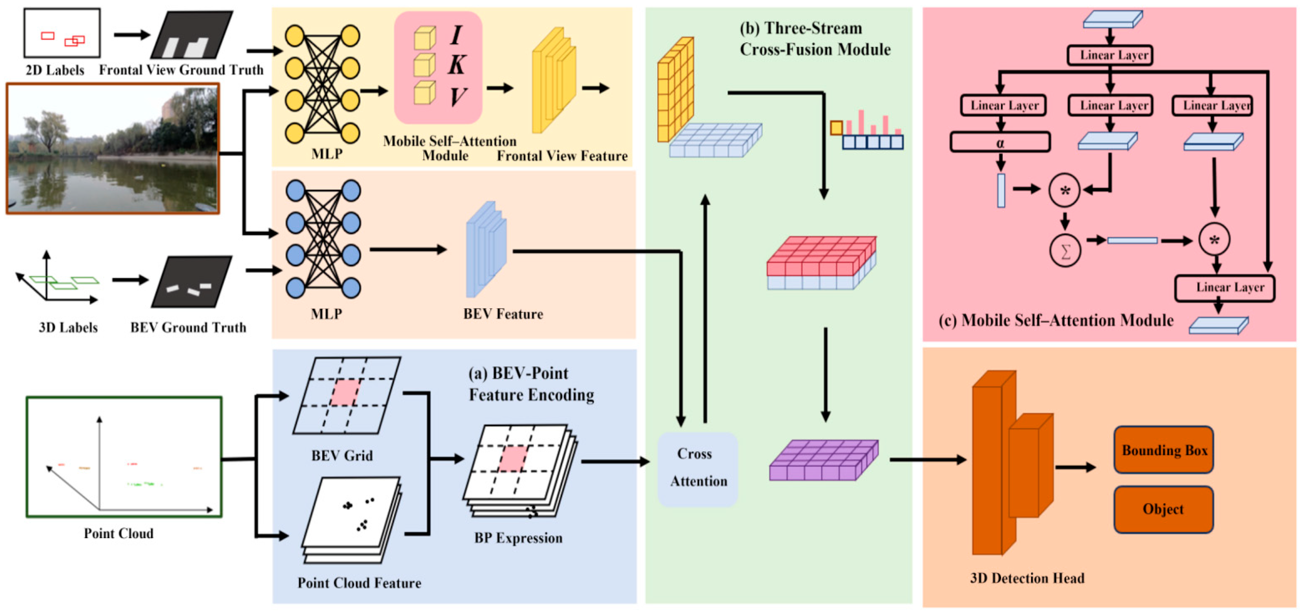
In response to the need for comprehensive 3D object data in USVs operations, the engineering challenges of deploying millimeter-wave imaging systems, and the degradat the production stage. Considering the limitation of multimodal data quality in complex water environments, we propose RCF-Free—a weak-calibration 3D object detection algorithm that fuses millimeter-wave radar and camera data. As illustrated in Figure 1, the overall architecture consists of three core components, shown in subfigures (a), (b), and (c).

The model takes two inputs: images and radar point clouds. The image features are initially processed through two multi-layer perceptron (MLP) networks to obtain the front-view object mask and the BEV mask. The front-view mask is then refined using the Mobile Self-Attention Module (MAM) to extract detailed front-view image features. Simultaneously, the point cloud data is processed by the proposed BEV-Point encoding module to generate the radar feature map in the BEV perspective.

Subsequently, within the Triple-Path Cross-View Fusion module, the initial BEV features derived from images are fused with the radar BEV feature map via a cross-attention mechanism, producing an intermediate BEV representation. This representation is then fused with the refined front-view features through cross-view interaction, yielding the final BEV feature map. The final BEV feature map is fed into a detection head to predict 3D bounding boxes for surface objects.

3.1. Mobile Self-Attention Module

To enhance the perception of 3D structure under sparse and non-uniform point cloud distributions, the RCF-Free method employs a Separable Attention Aggregation module, also referred to as the Mobile Self-Attention Module (MAM). The MAM emphasizes salient regions during front-view feature extraction.

The MAM is built upon the Multi-Head Attention (MHA) mechanism [43]. Unlike conventional self-attention, MHA effectively captures long-range dependencies in image data, enabling it to model semantic relationships between distant regions and better represent spatial correlations among features. This leads to an improved understanding of the overall scene layout. However, due to the high computational cost of MHA, this work adopts a separable attention mechanism as a more efficient alternative [44].

For an input feature $x_o$, the separable attention processes it through three branches: the input branch $I$, the key branch $K$, and the value branch $V$. The input $x_o$ is first processed through a shared-weight linear layer to obtain $x$, after which it enters the three branches, along with an additional residual connection leading to the final output.

Branch I uses a linear layer with weights $W_I\in {\mathrm{R}}^{\mathrm{d}}$ to map each d-dimensional token in $x$ to a scalar. The weights $W_I$ act as latent nodes L in the graph. This linear projection is an inner product operation used to compute the distance between the latent token L and $x$, resulting in a k-dimensional vector. The Softmax function is then applied to this k-dimensional vector to generate context scores $c_s\in {\mathrm{R}}^k$. Unlike the MHA, which computes attention scores for each token relative to all k tokens, the proposed method calculates context scores $c_s$ relative to only one latent token L, reducing the computational cost of calculating attention scores from $O(k^2)$ to $O(k)$. The context scores $c_s$ are used to compute the context vector $c_v$. Specifically, the key branch K, with weights $W_K\in {\mathrm{R}}^{\mathrm{d}\times \mathrm{d}}$, linearly projects the input x into d-dimensional space to produce the output $x_K\in {\mathrm{R}}^{\mathrm{k}\times \mathrm{d}}$. The context vector $c_v\in {\mathrm{R}}^{\mathrm{d}}$ is calculated by weighted summation of $x_K$, as shown below.

$$c_v=\sum _{i=1}^k{c}_s(i)x_K(i)$$

(1)

The contextual information encoded in $c_v$ will be shared with all tokens in x. To achieve this, the value branch V, with weights $W_V\in {\mathrm{R}}^{d\times d}$, linearly projects the input x into d-dimensional space. The output $x_V\in {\mathrm{R}}^{k\times d}$ is then obtained after applying the ReLU activation function. After this step, the contextual information in $c_v$ is propagated to $x_V$ through element-wise broadcasting multiplication. The resulting output is then fed into another linear layer with weights $W_O\in {\mathrm{R}}^{\mathrm{d}\times \mathrm{d}}$ to produce the final output $y\in {\mathrm{R}}^{\mathrm{k}\times \mathrm{d}}$.

In summary, after the first linear layer, the output of MAM can be defined as follows:

$$y=x+\left(\sum \left(\sigma \left(x{W}_I\right)\ast x{W}_K\right)\ast \mathrm{R}\mathrm{e}\mathrm{L}\mathrm{U}\left(x{W}_V\right)\right)W_O$$

(2)

where σ denotes the activation function, and ∗ represents the element-wise multiplication.

3.2. BEV-Point Feature Encoding

On the input side of the algorithm, for image input, we use two MLPs to achieve viewpoint decoupling from perspective view to front view and BEV. In this process, the network learns to decouple the perspective view features into FV and BEV features. The decoupled features are supervised by foreground segmentation labels generated based on 3D bounding box labels, without additional annotation costs, and within the weak calibration setting.

In the common field of unmanned ships, millimeter wave radar and cameras are mostly placed in the same location (or at a small distance) and detect the same direction. Based on this, we assume that the position of the millimeter wave radar and camera is a standard configuration. BEV image grid indexing formulas is as follows:

$$x_{grid}={\displaystyle \frac{x-x_{min}}{x_{max}-x_{min}}}\times N$$

(3)

$$y_{grid}=N-{\displaystyle \frac{y-y_{min}}{y_{max}-y_{min}}}\times N$$

(4)

In our method, N = 256, $y_{min}=x_{min}=-45,y_{max}=x_{max}=45$.

For point clouds input, to fully leverage information from millimeter-wave radar point clouds and efficiently generate BEV representations, this paper introduces the BEV-Point Encoder. This module encodes point cloud data into a grid-structured feature map through BEV projection and multi-modal feature fusion. The encoder consists of three core stages: point cloud rasterization, multi-modal feature encoding, and adaptive normalization, followed by a convolutional neural network (CNN) for deep feature extraction.

The mathematical modeling of each stage is as follows:

(1)

Point Cloud Rasterization Projection

Given the original point cloud data $P=(x_i,y_i,z_i,v_i)\in {\mathrm{R}}^{1\times 4}(i=1,2,3\dots n)$, we first establish the mapping relationship from the BEV coordinate system to the grid coordinates. Let the perception range be $[-R,R]\times [-R,R]$ and the grid resolution be $S\times S$. The spatial resolution is calculated as: $r={\displaystyle \frac{2R}{S}}$. The point cloud coordinates (x, y) are then projected into the grid coordinate system through an affine transformation.

$$\left\{\begin{array}{c}{u}_i=\lfloor {\displaystyle \frac{{\mathrm{C}}_1{x}_i}{r}}+{\displaystyle \frac{S}{2}}\rfloor \\ \begin{array}{c}{v}_i=S-\lfloor {\displaystyle \frac{{\mathrm{C}}_2{y}_i}{r}}+{\mathrm{R}}_1\rfloor \end{array}\end{array}\right.$$

(5)

$u_i,v_i\in [0,S-1]$ are the discrete grid coordinates. The coefficients C1 and C2 are used to adjust the scaling factors along different axes, while the constant R1 is employed to implement a mirror flip of the coordinate axes.

(2)

Multi-Modal Feature Encoding

To fully exploit the geometric and physical properties of the point cloud, the BEV-Point module designs features in the form of a 3D tensor $F\in {\mathrm{R}}^{S\times S\times 3}$, which includes three modalities: height, density, and reflectivity. A sliding window of size 5 × 5 is used to traverse all grid cells. The central grid of the window is updated based on surrounding information to suppress noise caused by outliers. The updated weights are calculated using a Gaussian function:

$$w(\mathsf{\Delta }u,\mathsf{\Delta }v)=\mathit{exp}(-{\displaystyle \frac{{\mathsf{\Delta }u}^2+{\mathsf{\Delta }v}^2}{2{\sigma }^2}})(\sigma =1.5)$$

(6)

w represents the diffusion weight of the surrounding grid cells on the current grid cell, while Δu and Δv are the coordinate offsets. The expression $\mathit{exp}(-{\displaystyle \frac{{\mathsf{\Delta }u}^2+{\mathsf{\Delta }v}^2}{2{\sigma }^2}})(\sigma =1.5)$ (where σ = 1.5) is the exponential part of the Gaussian formula with a standard deviation of 1.5. The closer the nearby point is to the center, the greater the weight.

During the traversal process, features are updated through weighted accumulation. The density feature $G_c$ is initialized with the number of point clouds within the grid; the initial value of the height feature $G_z$ is the z-coordinate of the point; and the initial value of the reflection intensity $G_v$ is the reflection intensity value:

$$G_{\alpha }\left(u,v\right)\leftarrow G_{\alpha }\left(u,v\right)+{\alpha }_{\mathrm{i}}w\left(\mathsf{\Delta }u,\mathsf{\Delta }v\right), \alpha =c, z, v$$

(7)

(3)

Adaptive Normalization

To enhance the robustness of features against dynamic environments, a piecewise normalization strategy is designed. First, the height channel feature Fz is processed:

$$F_{\alpha }^{norm}=\mathrm{C}\mathrm{l}\mathrm{i}\mathrm{p}({\displaystyle \frac{G_{\alpha }(u,v)}{\mu {\alpha }^{98\%}-\mu {\alpha }^{2\%}}},\mathrm{0,1}), \alpha =c, z, v$$

(8)

$F_z^{norm}$ represents the normalized height feature, and ${\mu }_z^{p\%}$ denotes the p-th percentile of the height feature sorted in ascending order. The Clip function restricts the computed result of the first expression within the limits defined by the second expression (in this case, 0) and the third expression (in this case, 1). For the normalization of the density channel and the reflectivity (or velocity), the same processing method is applied.

Here, $F{c}^{norm}$ and $F{v}^{norm}$ represent the normalized density feature and the reflectivity (or velocity) feature, respectively, with ${\mu }_c^{98\%}$ and ${\mu }_v^{98\%}$ defined similarly to ${\mu }_z^{p\%}$.

After the above steps, a 2D format BEV feature map with three channels is finally generated:

$$I_{BEV}=[F_z^{norm},F_c^{norm},F_v^{norm}]\in [\mathrm{0,1}{]}^{S\times S\times 3}$$

(9)

Finally, $I_{BEV}$ passes through a CNN convolutional network structure to generate the final point cloud BEV features.

After acquiring the BEV image features and rasterized point cloud features (at this point, the image perception range is X-axis ± 45 m, Y-axis 0~90 m, with a corresponding raster resolution of 256 × 256; the rasterized point cloud coverage is 40 m × 40 m, combined with a raster resolution of 720 × 720 pixels), the final alignment is performed in the feature space. The radar features are downsampled to a spatial resolution of 16 × 16 through a Convolutional Neural Network (CNN), maintaining the same spatial dimension as the decoupled BEV features from the image, ensuring consistent correspondence at the feature level.

3.3. Triple-Path Cross-View Fusion

To achieve more effective integration of point cloud and image features, we designed a Triple-Path Cross-View Fusion module. This module performs three-way fusion of the front-view feature map, the image-derived BEV feature map, and the point cloud BEV feature map encoded by the BEV-Point encoder. By comprehensively comparing feature discrepancies across these branches and integrating them, the module reconstructs complete 3D object profiles. Inspired by [45], this approach enables 3D object perception without relying on external parameters, thereby avoiding calibration errors that may degrade data quality and network performance.

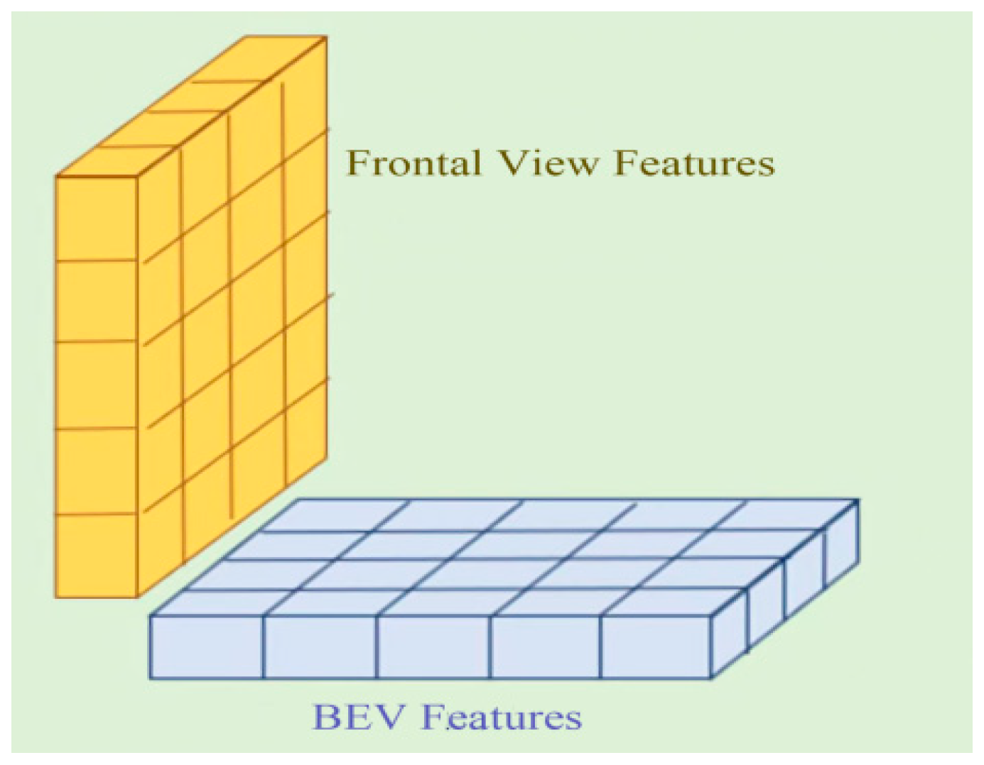
BEV features provide an effective representation of the scene layout from a top-down perspective. However, due to the inherent loss of information along the z-axis—especially under the weak calibration setting—3D detection performance can be limited. Thus, incorporating front-view features is essential for enhancing BEV representations. The primary challenge lies in establishing accurate correspondences between these orthogonal views.

As depicted in Figure 2, the front-view and BEV features exhibit an orthogonal relationship. Fusion of such feature pairs typically follows two paradigms. The first approach, similarity-based global fusion (SGF), operates under the assumption that features corresponding to the same object should be similar across views. While conceptually straightforward, SGF entails high computational costs. The second approach, condense-push fusion (CPF), reduces the matching search space by first compressing front-view features along the z-axis and then employing geometric constraints to propagate the fused features along the y-axis. However, both methods are generally applied to visual-only features and may suffer from unreliable BEV representations under challenging lighting conditions, such as those frequently encountered on water surfaces.

To combine the benefits of both CPF and SGF while overcoming the drawbacks of vision-only methods in complex illumination, we propose a similarity-based fusion module, SCF, which is inspired by [46]. This module employs a cross-attention mechanism to integrate outputs from the BEV-Point encoder and the visual encoder, producing high-quality BEV feature maps. Guided by geometric constraints, it effectively matches BEV and front-view features based on semantic and spatial similarity.

First, the image BEV feature map and the point cloud BP-encoded BEV feature map will be input into the cross-attention module [47]. Given the image BEV feature $F_P\in R^{H\times W\times C}$ and the point cloud BEV feature $F_I\in {\mathrm{R}}^{\mathrm{H}\times \mathrm{W}\times \mathrm{C}}$, the computation process is defined as follows:

$$\mathrm{C}\mathrm{r}\mathrm{o}\mathrm{s}\mathrm{s}\mathrm{A}\mathrm{t}\mathrm{t}\left(F_P,F_I\right)=\mathrm{Softmax}\left({\displaystyle \frac{Q_P{K}_I^T}{\sqrt{d_k}}}\right)V_I$$

(10)

where $Q_P=F_P{W}_P^Q$, $K_I=F_I{W}_I^K$, and $V_I=F_I{W}_I^V$, with $W_P^Q$, $W_I^K\mathrm{and}{W}_I^V$, serving as the parameter matrices for each modality. CrossAtt refers to the cross-attention module [45], and the Softmax function is a common activation function that normalizes the output values to the range of 0–1, ensuring that their sum equals 1. This mechanism allows the point cloud features to adaptively aggregate information from relevant image regions.

In the corresponding process of RCF-Free, the computation of the cross-attention module is executed, and a residual connection is introduced before the feature output to preserve the original point cloud feature information:

$$F_{out}=F_P+\mathrm{C}\mathrm{r}\mathrm{o}\mathrm{s}\mathrm{s}\mathrm{A}\mathrm{t}\mathrm{t}(F_P,F_I)$$

(11)

This residual structure can effectively alleviate the gradient vanishing problem while preserving the rich texture and color information in the image features. Subsequently, the front-view features and BEV features are fused.

To reduce computational costs, the compressed feature $f_c=\mathrm{M}\mathrm{e}\mathrm{a}\mathrm{n}\mathrm{P}\mathrm{o}\mathrm{o}\mathrm{l}\mathrm{i}\mathrm{n}\mathrm{g}(f_{fv})$ is used for feature fusion, where MeanPooling refers to the average pooling operation along the z-axis. The similarity $s_{ij}$ is measured through the dot product:

$$s_{ij}=⟨f_{c_i},f_{be{v}_{ij}}⟩$$

(12)

i is the index along the x-axis, and j is the index along the y-axis. The calculated similarity is used as fusion weights to leverage the compressed front-view features $f_c$ to enhance the BEV features $f_{bev}$:

$$f_e=\mathrm{C}\mathrm{o}\mathrm{n}\mathrm{v}\left(\mathrm{C}\mathrm{o}\mathrm{n}\mathrm{c}\mathrm{a}\mathrm{t}\left(f_{bev},s\ast f_c\right)\right)$$

(13)

Here, Conv and Concat represent convolution and concatenation operations, respectively, with $f_e$ being the output features.

The similarity distribution between orthogonal views along the y-axis implicitly encodes depth information, as features closer to the true depth exhibit higher cross-view similarity. The proposed Similarity-based Cross-Fusion (SCF) module effectively combines similarity-based global fusion (SGF) with compressed push fusion (CPF). This design effectively bridges orthogonal views and improves geometric consistency without relying on explicit depth supervision. Moreover, it facilitates spatial alignment by encouraging corresponding features to reside in the same x-column, thereby improving geometric consistency across views.

3.4. Loss Function

In the loss function setup of this algorithm, the loss functions for generating the front-view and BEV masks using two MLP networks, as well as for performing the 3D object detection task from the BEV perspective, are set as follows:

$$\mathrm{L}\mathrm{o}\mathrm{s}\mathrm{s}=L_{box}+\stackrel{.}{L_{cls}}+L_{obj}$$

(14)

$L_{box}$ is the bounding box localization loss, $L_{cls}$ is the classification loss, and $L_{obj}$ is the confidence loss. The $L_{box}$ primarily calculates the errors in the position and size of the detection box, which can be represented as follows:

$$L_{box}={\lambda }_{coord}\sum _{i=0}^{S^2}\sum _{j=0}^B{1}_{i,j}^{\mathrm{o}\mathrm{b}\mathrm{j}}\cdot {\mathrm{l}}_{i,j}^{\mathrm{b}\mathrm{o}\mathrm{x}}$$

(15)

Here, ${\lambda }_{coord}$ is the weight for the bounding box regression loss, $S^2$ is the total number of anchors, B is the number of bounding boxes for each anchor, and $1_{i,j}^{\mathrm{o}\mathrm{b}\mathrm{j}}$ indicates whether the j-th anchor box at the i-th anchor contains an object. This value is 1 if it contains an object (positive sample) and 0 otherwise (negative sample). The loss ${\mathrm{l}}_{\mathrm{i},\mathrm{j}}^{\mathrm{b}\mathrm{o}\mathrm{x}}$ represents the bounding box loss for the j-th bounding box at the i-th anchor, and can be expressed as the CIOU (Complete Intersection over Union) loss: CIOU [11]. $L_{cls}$ is used to determine the category of the object and can be represented as follows:

$$L_{cls}={\lambda }_{class}\sum _{i=0}^{S^2}\sum _{j=0}^B{1}_{i,j}^{\mathrm{o}\mathrm{b}\mathrm{j}}\cdot \mathrm{B}\mathrm{C}\mathrm{E}(p_{i,j}^{cls},t_{i,j}^{cls})$$

(16)

λ_class is the weight for the classification loss, $t_{i,j}^{cls}$ represents the ground truth probability for the class of the j-th bounding box at the i-th anchor, and $p_{i,j}^{cls}$ is the predicted class probability. BCE denotes the binary cross-entropy loss function. The loss $L_{obj}$ is used to determine whether the detection box contains an object:

$$L_{obj}={\lambda }_{obj}\sum _{i=0}^{S^2}\sum _{j=0}^B\mathrm{B}\mathrm{C}\mathrm{E}(p_{i,j}^{obj},t_{i,j}^{obj})$$

(17)

${\lambda }_{obj}$ is the weight for the confidence loss, $p_{i,j}^{obj}$ represents the confidence of the predicted label, and $t_{i,j}^{obj}$ is the confidence of the ground truth label.

When performing conventional 3D object detection, the following loss function is used to train the algorithm:

$$L_{detect}={\displaystyle \frac{1}{N_s}}[\sum _i{L}_{cls}(p_i,l_i^{\ast }(\mathrm{Io}{\mathrm{U}}_i))+\Gamma (\mathrm{Io}{\mathrm{U}}_i\ge {\vartheta }_{\mathrm{reg} })\sum _i{L}_{reg}({\xi }_i,t_i^{\ast })]$$

(18)

The classification loss $L_{cls}()$ uses Focal Loss, while the regression loss $L_{reg}()$ employs Huber Loss [47]. $p_i^a$ is the output for the classification task, and $c_i^{\ast }$ is the label for the classification task; ${\xi }_i^a$ is the output for the regression task, and $t_i^{\ast }$ is the label for the regression task. The notation $\Gamma (c_i^{\ast }\ge 1)$ means that the regression loss is computed only for foreground anchor boxes.

The term $\mathrm{Io}{\mathrm{U}}_i$ represents the intersection-over-union (IoU) between the i-th proposed box and its corresponding ground truth box. ${\vartheta }_H$ and ${\vartheta }_L$ indicate the upper and lower thresholds for the IoU between foreground and background. $N_s$ denotes the number of proposal boxes sampled during the training phase, and $\Gamma (\mathrm{Io}{\mathrm{U}}_i\ge {\vartheta }_{\mathrm{reg} })$ means that only proposal boxes with an IoU above the threshold are included in the computation of the loss function.

4. Experiments

4.1. Datasets

Our experimental evaluation utilizes the following datasets:

4.1.1. Water Surface Datasets

Since existing multimodal aquatic datasets only provide 3D point clouds without annotations in 3D space, they cannot be directly applied to 3D object detection tasks. To address this limitation, we utilized the point cloud data from two existing datasets and leveraged their projection relationships with corresponding image modalities to generate accurate BEV 3D bounding box annotations. This process led to the construction of two new benchmark datasets: FloW-BEV and WaterScenes-BEV.

(1)

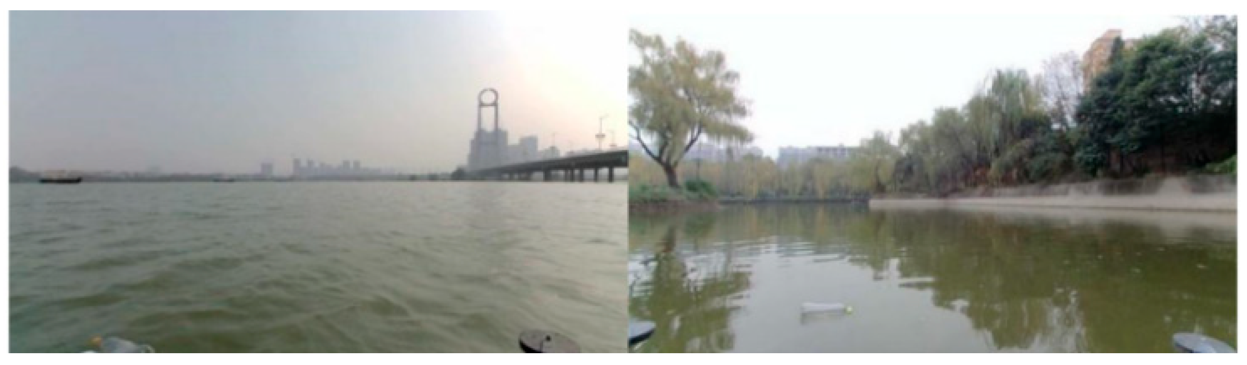
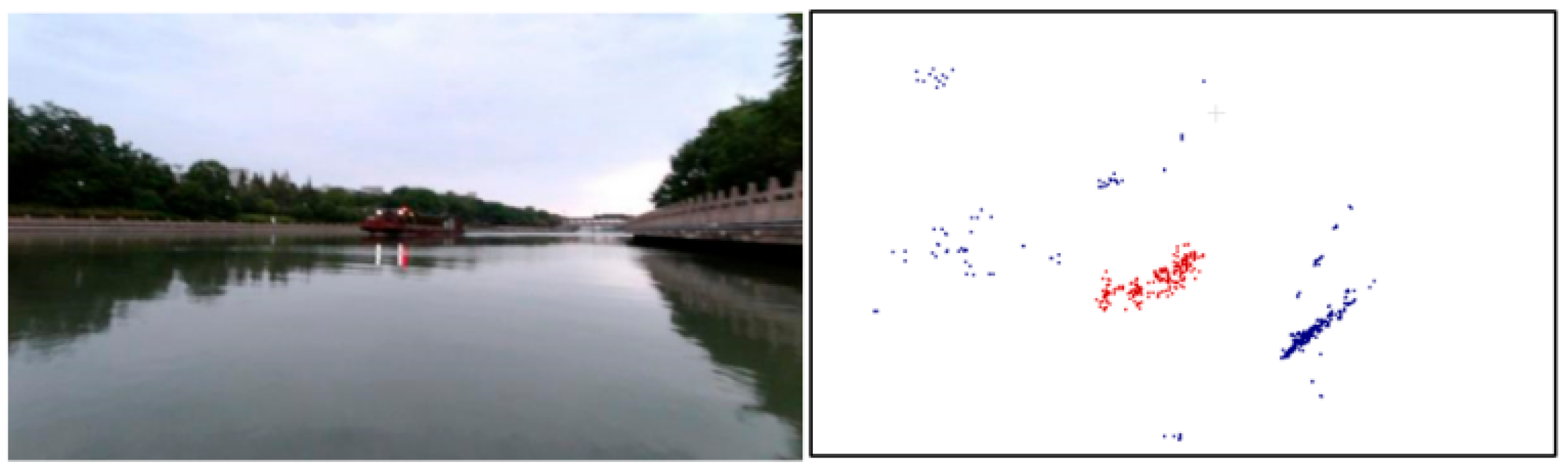
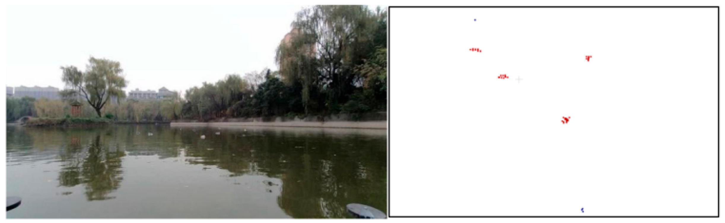
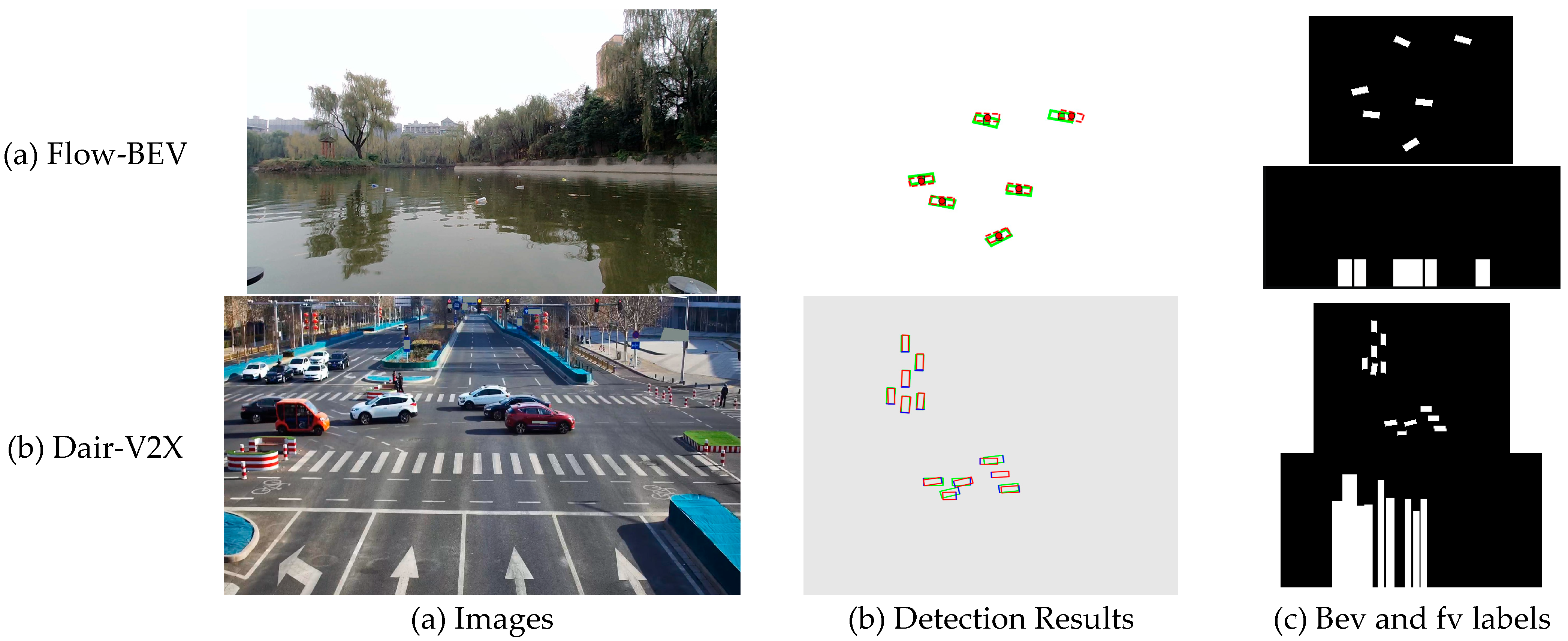
FloW-BEV: Reconstructed from the FloW-RI dataset [6], it provides 3D annotations for its 2000 frames of image and point cloud data. Examples of this dataset are shown in Figure 3 and Figure 4.

(2)

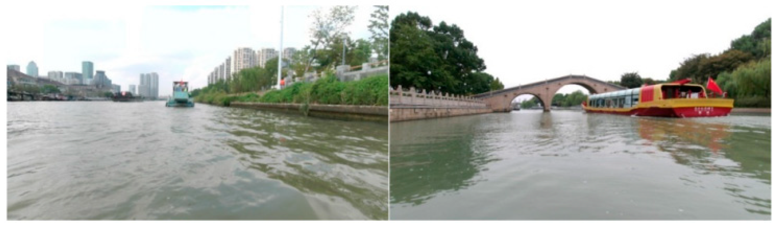
WaterScenes-BEV: Reconstructed from the WaterScenes dataset [24], it provides 3D annotations for a subset of its extensive multimodal data collection. Examples of this dataset are shown in Figure 5 and Figure 6.

To ensure high-quality annotations, our labeling pipeline follows a structured three-stage process comprising initial annotation, image-projection verification, and temporal-context cross-validation. In the initial stage, annotators utilize an enhanced version of the LabelCloud tool, extended with the Qt library to better handle millimeter-wave radar point clouds. Point clouds are stacked along the z-axis to form a BEV representation, and preliminary 3D bounding boxes are drawn based on the shape, density, and contour of point clusters. The enhanced tool assists this process through real-time filtering and cluster visualization, mitigating challenges posed by sparse and noisy radar data.

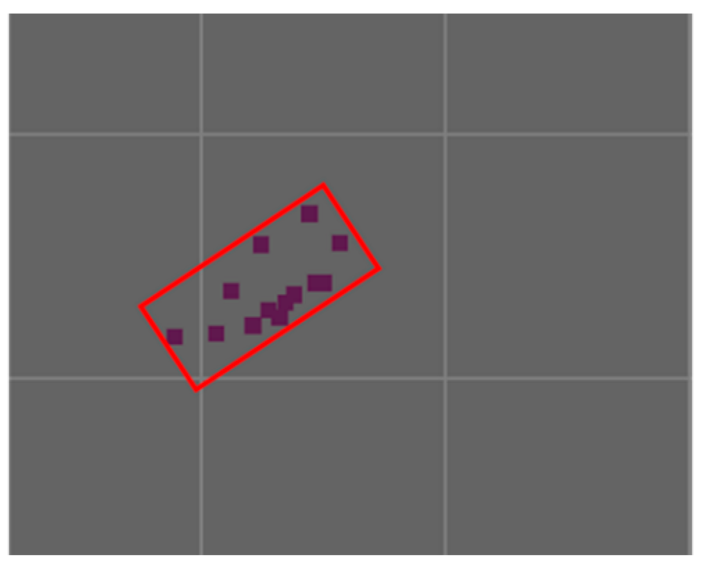
Following the initial placement, each 3D bounding box enters the image-projection verification stage, a critical step for establishing cross-modal alignment. Our tool automatically projects the current BEV box onto the precisely time-synchronized RGB image in a side-by-side interactive panel. Annotators meticulously examine the correspondence between the projected 2D polygon and the visible object’s texture, edges, and overall silhouette in the camera view. Discrepancies often arise from point cloud sparsity or lateral occlusion. When adjustment is needed, annotators can manipulate the 3D box’s parameters—not only its (x, y) center and yaw orientation but also its length and width—directly within the image view via intuitive click-and-drag handles. The system performs real-time inverse projection to update the BEV representation instantly, allowing for an iterative refinement loop. This closed-loop visual verification guarantees that the final 3D annotation is geometrically coherent with the 2D visual evidence, as illustrated in Figure 7 for a representative floating object.

Finally, to ensure temporal smoothness and label integrity across sequences, we employ a targeted multi-frame cross-validation check. For dynamic objects, the tool loads a short sequence (typically 3–5 frames centered on the current frame). Annotators review the object’s trajectory by visualizing the annotated boxes across these frames simultaneously, checking for physical plausibility in motion (consistent velocity, reasonable acceleration) and shape stability. This process identifies and corrects temporal outliers, such as a box that suddenly jumps due to a single-frame point cloud artifact, and ensures that partially occluded objects in one frame are labeled consistently with their visible states in adjacent frames. This three-tiered approach—combining sensor-aware BEV annotation, interactive image-geometry verification, and temporal consistency review—produces a dataset with annotations that are geometrically accurate, visually grounded, and temporally coherent, forming a reliable foundation for training and evaluating perception models.

4.1.2. DAIR-V2X Dataset

To validate the generalization capability of our algorithm, we also evaluated it on the public DAIR-V2X-I dataset [48] from the autonomous driving domain. This dataset provides 10,084 synchronized image-point cloud frames captured in diverse real-world road environments, with comprehensive 2D and 3D annotations. It allows for benchmarking under various conditions (e.g., weather, illumination).

4.2. Experimental Setup and Evaluation Metrics

4.2.1. Experimental Setup

The algorithm training and testing hardware platform is NVIDIA RTX A6000, implemented using the PyTorch 1.13.1 framework. The algorithm training and testing hardware platform is NVIDIA RTX A6000, and the key parameter settings are shown in

Table 1. Some Key Parameters Set during Model Training.

Parameters	Setup
Initial learning rate	2 × 10−5
Weight decay	2 × 10−6
Batch size	6
Input image size	1024 × 1024
Radar mask size	720 × 720
Optimizer	Adam (betas = (0.9, 0.999), eps = 1 × 10−8)

. In this algorithm, the image input is processed using the ResNet-18 backbone pre trained by ImageNet, and the mask image is classified using different grayscale values, where 0 is the background.

Flow-BEV and WaterScenes-BEV correspond to scenarios with floating objects on water and vessels on water, The datasets are divided into training and testing sets at a ratio of 8:2, with a total of 400 iterations. DAIR-V2X-I dataset corresponds to intersection scenarios in autonomous driving, with a training set and testing set divided in a 7:3 ratio and a total of 200 iterations.

For the loss function, during the training and validation on the water surface dataset in the experiment, BEV object detection was performed, thus the loss functions defined in Equations (14)–(17) was adopted. For the Dair-V2x dataset, the loss function of formula 18 was used for conventional 3D detection.

In the related experiments of CBR and RCF-Free, we fixed almost all random numbers, with the random seed of PyTorch set to 42.

Evaluation Metrics: In this paper, we use mean Average Precision mAP, ${\mathrm{m}\mathrm{A}\mathrm{P}}_{\mathrm{B}\mathrm{E}\mathrm{V}}$, ${\mathrm{m}\mathrm{A}\mathrm{P}}_{3\mathrm{D}}$ and ${\mathrm{m}\mathrm{I}\mathrm{O}\mathrm{U}}_{\mathrm{B}\mathrm{E}\mathrm{V}}$ metrics to quantitatively evaluate the performance of the algorithm on the test sets of the datasets. The mean Average Precision (mAP) is the average of the APs for all categories, as shown in Equation (19). Specifically, mAP50 refers to the average AP for all categories when the IoU (Intersection over Union) value between the predicted boxes and the ground truth boxes is greater than 0.5.

$$\mathrm{m}\mathrm{A}\mathrm{P}={\displaystyle \frac{1}{N}}\sum _{i=1}^{N}A P_i$$

(19)

${\mathrm{m}\mathrm{A}\mathrm{P}}_{\mathrm{B}\mathrm{E}\mathrm{V}}$ are defined similarly to Equation (20), but the IoU calculations for the detected samples are extended to the 3D space, and its core lies in the fact that the IoU is computed within the BEV plane. Specifically, for each predicted 3D bounding box and its corresponding ground truth box, they are first projected onto the ground plane (X-Y plane) along the Z-axis (vertical direction), resulting in two 2D rectangles. Subsequently, the Intersection over Union (IoU) between these two 2D rectangles on the BEV plane is calculated. Finally, ${\mathrm{m}\mathrm{A}\mathrm{P}}_{\mathrm{B}\mathrm{E}\mathrm{V}}$ is defined as the mean of the Average Precision (AP) values for all object categories at a specified BEV IoU threshold (typically 0.5). The calculation process can be formalized as follows:

For a matched pair of predicted box $B_{pred}=(x,y,l,w,\theta )$ and ground truth box $B_{gt}=({ x}_{gt},{ y}_{gt},{ l}_{gt},{ w}_{gt},{ \theta }_{gt})$ (containing center location, length, width, and orientation), ignoring their height information, compute the IoU of their 2D projected areas on the X-Y plane:

$${IoU}_{BEV}={\displaystyle \frac{Area(B_{pred}^{2D}\cap B_{gt}^{2D})}{Area(B_{pred}^{2D}\cup B_{gt}^{2D})}}$$

(20)

$${mAP}_{BEV}={\displaystyle \frac{1}{N}}{\displaystyle \sum _{i=1}^N}{AP}_{BEV}^i$$

(21)

$B^{2D}$ represents the rectangular projection of the 3D bounding box onto the BEV plane.

${\mathrm{m}\mathrm{I}\mathrm{O}\mathrm{U}}_{\mathrm{B}\mathrm{E}\mathrm{V}}$ represents the average IoU value between the ground truth boxes and the detected boxes for all samples.

4.2.2. Model Hyperparameter Setup

To determine a robust configuration for the model, this study analyzed several key hyperparameters, primarily including loss function weights, the backbone network, and the BEV spatial resolution.

As shown in Equation (14), the loss function of our method consists of three parts: the bounding box regression loss $L_{box}$, the classification loss $L_{cls}$ and the object confidence loss $L_{obj}$. Experiments on the FloW-BEV dataset indicate that setting the weights for all three parts to 1 allows the model to converge well and achieve excellent performance. To evaluate its sensitivity, we tested different weight combinations. The results show that adjusting the weights has a relatively limited impact on the final performance. Among them, reducing the weight of $L_{obj}$ has the most significant effect, but it only decreases $\mathrm{m}\mathrm{A}{\mathrm{P}}_{\mathrm{B}\mathrm{E}\mathrm{V}}$ and mIOU by approximately 0.4% and 0.3%, respectively. Although increasing the weight of $L_{obj}$ to 3 on the WaterScenes-BEV dataset led to an improvement of about 0.2% in both $\mathrm{m}\mathrm{A}{\mathrm{P}}_{\mathrm{B}\mathrm{E}\mathrm{V}}$ and mIOU, this setting significantly increases the difficulty of model convergence. For instance, on the FloW-BEV dataset, it requires approximately 100 additional training epochs to achieve comparable results to the original weights, with no significant further gains observed. Therefore, considering the trade-off between performance and training stability, this study adopts (1,1,1) as the default loss weight configuration.

For backbone, considering the requirements for computational efficiency and real-time performance on unmanned surface vehicle platforms, this study selects ResNet-18, which has a smaller parameter count, as the image backbone network. Experiments confirm that while using a larger backbone network (e.g., ResNet-34) can bring slight accuracy improvements, it significantly increases computational overhead and latency.

The BEV spatial resolution in the view decoupling module directly affects the granularity of the top-view features decoupled from the image. We compared the detection performance under different resolution settings on the FloW-BEV dataset, as shown in

Table 2. The comparative experiments on the FloW-BEV Dataset under different BEV resolutions.

BEV Resolution	$\mathbf{m}\mathbf{A}{\mathbf{P}}_{\mathbf{B}\mathbf{E}\mathbf{V}}/\%$	$\mathbf{mIOU}/\%$
4	58.0	44.9
8	60.5	47.2
16	59.6	46.8

. Experiments show that setting the resolution to 8 yields the optimal $\mathrm{m}\mathrm{A}{\mathrm{P}}_{\mathrm{B}\mathrm{E}\mathrm{V}}$ and mIOU. When the resolution is reduced to 4, the feature map becomes too coarse, leading to loss of detail and performance degradation. When the resolution is increased to 16, the feature map becomes finer, but it may introduce more irrelevant noise or increase the difficulty of model optimization, preventing further performance gains and even causing a slight decline. Therefore, a resolution of 8 is determined to be the optimal balance between feature representation capability and model robustness.

4.3. Quantitative Analysis

4.3.1. Comparison Experiments

(1)

Comparison Experiments on the Reconstructed Datasets FloW-BEV and WaterScenes-BEV

To evaluate the efficacy of the proposed 3D object detection algorithm RCF-Free in surface environments, a comparative analysis of detection performance was conducted on the self-constructed dataset FloW-BEV. The results are summarized in

Table 3. Comparison of Detection Performance of Different Methods on the FloW-BEV Dataset (IoU = 0.5), the number after ± is the standard deviation. Among these algorithms, FE-YOLOv5n, YOLOv9s-Hungarian and MFNet are decision-level-fusion methods.

Methods	$\mathbf{m}\mathbf{A}{\mathbf{P}}_{\mathbf{B}\mathbf{E}\mathbf{V}}/\%$	$\mathbf{mIOU}/\%$
FE-YOLOv5n [49]	27.4	30.1
YOLOv9s-Hungarian	24.5	30.0
MFNet	31.0	44.9
CBR [46]	56.9	45.0
RCF-Free	60.5 ± 0.6	47.2 ± 0.7

.

CBR is adopted as the baseline model in this study. As illustrated in Table 3, RCF-Free achieves the highest performance across both evaluation metrics on the validation set of the FloW-BEV dataset. Specifically, compared to FE-YOLOv5n, YOLOv9s-Hungarian, MFNet, and CBR, RCF-Free exhibits improvements in $\mathrm{m}\mathrm{A}{\mathrm{P}}_{\mathrm{B}\mathrm{E}\mathrm{V}}$ of 33.1%, 36.0%, 29.5%, and 3.6%, respectively. Corresponding gains in mIOU are 17.1%, 17.2%, 2.3%, and 2.2%. These results underscore the superior capability of RCF-Free in detecting floating objects on water surfaces.

It is also observed that the expanded pixel strategy used in FE-YOLOv5n contributes to certain performance improvements in such scenarios, yielding noticeably higher accuracy than the YOLOv9s-Hungarian approach. However, conventional decision-level fusion methods still exhibit limitations. The extracted point cloud bounding boxes tend to be coarse, potentially incorporating adjacent points erroneously and thus reducing $\mathrm{m}\mathrm{A}{\mathrm{P}}_{\mathrm{B}\mathrm{E}\mathrm{V}}$. In contrast, both the CBR algorithm and RCF-Free show substantially better performance in terms of $\mathrm{m}\mathrm{A}{\mathrm{P}}_{\mathrm{B}\mathrm{E}\mathrm{V}}$.

Even in cases of misdetection, the point cloud boxes obtained through decision-level fusion still partially overlap with ground truth boxes. Therefore, for small objects, RCF-Free yields a notable improvement in $\mathrm{m}\mathrm{A}{\mathrm{P}}_{\mathrm{B}\mathrm{E}\mathrm{V}}$, with a more moderate yet clear increase in mIOU. Overall, the proposed method exhibits superior comprehensive performance.

In addition, to test the sensitivity of the model to random initialization, we removed the restriction on the random seed in PyTorch and conducted 8 rounds of complete training, selecting the optimal model as the result each time. In the test results, the average $\mathrm{m}\mathrm{A}{\mathrm{P}}_{\mathrm{B}\mathrm{E}\mathrm{V}}$ is 60.5%, with a maximum of 61.3% and a minimum of 59.8%. The average mIOU is 47.2%, with a maximum of 48.1% and a minimum of 46.3%. The standard deviation of $\mathrm{m}\mathrm{A}{\mathrm{P}}_{\mathrm{B}\mathrm{E}\mathrm{V}}$ is 0.5%, and the standard deviation of mIOU is 0.7%. We also calculated the standard deviation on waterscene Bev and dair-v2x-i respectively.

Table 4. Comparison of Detection Performance of Different Methods on the WaterScenes-BEV Dataset (IoU = 0.5), the number after ± is the standard deviation. Among these algorithms, FE-YOLOv5n, YOLOv9s-Hungarian and MFNet are decision-level-fusion methods.

Methods	$\mathbf{m}\mathbf{A}{\mathbf{P}}_{\mathbf{B}\mathbf{E}\mathbf{V}}/\%$	$\mathbf{mIOU}/\%$
FE-YOLOv5n	5.2	20.1
YOLOv9s-Hungarian	5.3	20.2
MFNet	6.8	22.8
PointPillars [50]	46.6	39.3
BEVFormer [51]	71.6	56.1
BEVDepth [33]	64.2	47.4
CBR	67.4	52.9
RCF-Free	69.3 ± 0.4	55.3 ± 0.3

presents a comparative assessment of RCF-Free against other detection methods on the reconstructed WaterScenes-BEV dataset. The results affirm the high accuracy of RCF-Free in detecting water vessels. It significantly outperforms decision-level fusion methods (FE-YOLOv5n, YOLOv9s-Hungarian, MFNet) and the point-cloud-based detector PointPillars, with $\mathrm{m}\mathrm{A}{\mathrm{P}}_{\mathrm{B}\mathrm{E}\mathrm{V}}$ improvements of 64.1%, 63.0%, 62.5%, and 22.7%, respectively. This substantial gap underscores the challenge that sparse, noisy maritime radar point clouds pose for geometry-only or late-fusion approaches. By leveraging high-quality image features enhanced with point cloud information through its fusion architecture, RCF-Free also surpasses the vision-only baseline CBR by 1.9% in $\mathrm{m}\mathrm{A}{\mathrm{P}}_{\mathrm{B}\mathrm{E}\mathrm{V}}$ and 2.4% in mIOU, demonstrating the clear benefit of multimodal integration.

The inclusion of state-of-the-art BEV detection methods reveals interesting insights. PointPillars, designed for denser LiDAR point clouds, performs poorly in this sparse radar scenario. Both BEVFormer and BEVDepth, which rely on precise calibration, achieve strong results. Notably, BEVFormer exceeds RCF-Free’s score, while BEVDepth performs slightly worse—a trend opposite to their ranking on the DAIR-V2X autonomous driving dataset. This discrepancy can be attributed to the domain-specific optimizations of these methods. BEVDepth’s design, particularly its depth estimation module (LSS), is heavily optimized for the structural and depth distribution priors of ground-based autonomous driving scenes (e.g., cars, roads). The aquatic environment, with its flat surface, different target size distributions, and unique clutter patterns, represents a significant domain shift where these priors may not hold, leading to suboptimal performance. In contrast, BEVFormer’s transformer-based view transformation mechanism demonstrates better generalization. Nevertheless, RCF-Free, without requiring precise calibration parameters, achieves competitive performance that is on par with these calibration-dependent state-of-the-art methods, highlighting its remarkable practical value and robustness in real-world aquatic deployment where calibration is unreliable.

(2)

Comparison Experiments on the Public Dataset DAIR-V2X-I

To further evaluate the effectiveness and generalization capability of the proposed algorithm, we compared RCF-Free with several state-of-the-art 3D object detection methods on the public autonomous driving dataset DAIR-V2X-I. The results are summarized in

Table 5. Comparison of Detection Performance of Different Methods. mAP_3D, IoU = 0.5, L represents LiDAR, C represents vision, LC represents multi-modality. CBR and RCF-Free do not require accurate calibration parameters. All scores are reported in percentage (%), the number after ± is the standard deviation.

Methods	Modal	Easy/%	Moderate/%	Hard/%
PointPillars [50]	L	63.1	54.0	54.0
Second [52]	L	71.5	54.0	54.0
MVX-Net [53]	L&C	71.0	53.7	53.8
ImVoxelNet [54]	C	44.8	37.6	37.6
BEVFormer [51]	C	61.4	50.7	50.7
BEVDepth [33]	C	75.5	63.6	63.7
BEVHeight [55]	C	77.8	65.8	65.9
BEVSpread [56]	C	79.1	66.8	66.9
CUDA-V2XFusion [57]	L&C	82.1	69.7	69.8
UncertainBEV [58]	L&C	84.9	70.3	70.3
CBR	C	72.0	60.1	60.1
RCF-Free (Ours)	L&C	73.3 ± 0.4	61.2 ± 0.3	61.2 ± 0.3

.

As shown in Table 5, RCF-Free achieves $\mathrm{m}\mathrm{A}{\mathrm{P}}_{3\mathrm{D}}$ improvements of 1.3%, 1.1%, and 1.1% over the baseline CBR across easy, moderate, and hard task difficulty levels, respectively. Under weak calibration setting, RCF-Free ranks third overall among all methods in all three difficulty categories. It outperforms calibration-dependent radar-based methods by margins of at least 1.8%, 7.2%, and 7.2% across the three levels. Compared to multimodal methods that require calibration, the improvements are 2.3%, 7.5%, and 7.4%, respectively. Relative to vision-only methods relying on calibration, RCF-Free surpasses ImVoxelNet by 29.1%, 23.6%, and 23.6%, and BEVFormer by 11.9%, 10.5%, and 10.5%.

These results affirm that although RCF-Free is specifically designed for the unique challenges of aquatic environments, it generalizes effectively to terrestrial autonomous driving scenarios, exhibiting robust detection capability. It is important to contextualize this performance: while the absolute accuracy of RCF-Free remains below that of the latest calibration- and depth-supervised methods (e.g., BEVDepth, BEVHeight, and CUDA-V2XFusion), this comparison highlights a fundamental design trade-off. Methods like BEVDepth and CUDA-V2XFusion achieve superior performance by leveraging precise calibration and computationally intensive depth estimation networks, which incur high inference costs and pose challenges for real-time edge deployment. In contrast, RCF-Free forgoes this dependency, offering the significant advantage of operating without any accurate calibration parameters input, thereby eliminating associated deployment complexity, cost, and the risk of performance degradation from calibration drift.

Furthermore, this practicality is reflected in the model’s efficiency. The parameter count of RCF-Free is only about 2% larger than that of the CBR baseline (∼410 M vs. ∼400 M), and it is significantly more compact than networks incorporating heavy depth estimation modules (e.g., BEVHeight, ∼880 M). This compactness, combined with its weak-calibration design, makes RCF-Free particularly suitable for scalable and reliable deployment on resource-constrained platforms like USVs, where maintaining precise calibration is often impractical.

In summary, the comparison in Table 5 and the accompanying analysis serve to clearly position our contribution. RCF-Free is not designed to outperform all methods in idealized, calibrated settings but to deliver a robust, efficient, and readily deployable perception solution for calibration-constrained environments where the state-of-the-art, calibration-dependent methods cannot be reliably applied.

4.3.2. Ablation Experiment

To systematically validate the effectiveness of each proposed component, a comprehensive ablation study was conducted. As the baseline model CBR lacks a point cloud branch, the conventional approach of “removing a module” is not directly applicable for evaluating the multimodal fusion. Therefore, we designed the following model variants: RCF-Free-RI refers to the variant that incorporates the BEV-Point encoder for processing millimeter-wave radar point clouds and the Triple-Path Cross-View Fusion module for multi-modal feature integration. RCF-Free-RI-C, which incorporates the BEV-Point cloud encoder but does not use the Triple-Path Cross-View Fusion module, instead adopting a simple feature concatenation method similar to CBR to fuse point cloud features before the detection head. This variant tested the necessity of our proposed fusion architecture. RCF-Free-RI-MHA replaces the Mobile Self-Attention Module (MAM) in RCF-Free-RI with a standard Multi-Head Attention (MHA) mechanism to benchmark the efficiency advantage of MAM. RCF-Free denotes the complete proposed model, which further includes the MAM.

Results are summarized in

Table 6. The Result of Ablation Experiment.

Datasets	Methods	$\mathbf{m}\mathbf{A}{\mathbf{P}}_{\mathbf{B}\mathbf{E}\mathbf{V}}$/%	mIOU/%	FPS/Hz	Latency/ms
Flow-BEV	CBR	56.9	45.0	198.1	5.1
	RCF-Free-RI-C	57.2	45.4	98.3	10.2
	RCF-Free-RI	59.5	46.5	126.3	7.9
	RCF-Free-RI-MHA	60.1	46.7	105.9	9.4
	RCF-Free	60.5	47.2	121.6	8.2
WaterScenes-BEV	CBR	67.4	52.9
	RCF-Free-RI-C	66.7	53.1
	RCF-Free-RI	68.4	54.6
	RCF-Free-RI-MHA	67.6	54.0
	RCF-Free	69.3	55.3
		$\mathbf{m}\mathbf{A}{\mathbf{P}}_{\mathbf{3}\mathbf{d}}$/%
		Easy	Mod.	Hard
Dair-V2X	CBR	72.0	60.1	60.1
	RCF-Free-RI-C	68.5	56.8	56.8
	RCF-Free-RI	73.6	60.5	60.6
	RCF-Free-RI-MHA	73.1	60.7	60.7
	RCF-Free	73.3	61.2	61.2

, and we analyze them from three perspectives: accuracy, robustness, and efficiency. The comparison between RCF-Free-RI-Cand the baseline CBRis particularly revealing. On the FloW-BEV dataset, the fusion method of CBR can only bring a slight performance improvement (+0.3% $\mathrm{m}\mathrm{A}{\mathrm{P}}_{\mathrm{B}\mathrm{E}\mathrm{V}}$). More critically, on the DAIR-V2X dataset, this variant causes a significant performance drop ($\mathrm{m}\mathrm{A}{\mathrm{P}}_{3d}$ Easy decreases by 3.5%). This clearly indicates that in scenarios with larger-scale or richer point clouds (e.g., DAIR-V2X), a crude fusion strategy can introduce noise or lead to feature competition between modalities, thereby degrading the performance of the original visual model. In stark contrast, RCF-Free-RI, equipped with our proposed Triple-Path Cross-View Fusion module, achieves consistent improvements across all datasets. This strongly validates that our designed cross-view attention mechanism is crucial for achieving effective and beneficial multimodal fusion, rather than merely introducing additional features.

A decomposition of each module’s contribution is evident on the FloW-BEV dataset. RCF-Free-RI achieves a +2.6% gain in $\mathrm{m}\mathrm{A}{\mathrm{P}}_{\mathrm{B}\mathrm{E}\mathrm{V}}$ over CBR, attributable primarily to the effective representation of sparse point clouds by the BEV-Point encoder and the high-quality feature integration enabled by the Triple-Path Cross-View Fusion. Building upon this, incorporating the MAM to form the complete RCF-Free model delivers a further +1.0% $\mathrm{m}\mathrm{A}{\mathrm{P}}_{\mathrm{B}\mathrm{E}\mathrm{V}}$ improvement. This verifies that the MAM, by enhancing spatial contextual understanding, further refines the front-view visual features for more precise alignment with BEV features. A consistent trend of incremental gains from each module is also observed on the more complex WaterScenes-BEV dataset.

We further analyzed the model’s efficiency on the FloW-BEV dataset. Introducing the multimodal fusion core (RCF-Free-RI) inevitably increases computational cost while delivering significant accuracy gains, with latency rising from 5.1 ms to 7.9 ms. A key finding concerns the efficiency of our proposed lightweight MAM versus standard Multi-Head Attention (MHA). Comparing RCF-Free-RI-MHA and RCF-Free, both achieve comparable accuracy, but RCF-Free exhibits lower latency and higher FPS. This confirms that the MAM maintains powerful contextual modeling capabilities while offering superior computational efficiency. Ultimately, the complete RCF-Free model delivers the best detection accuracy with a latency of approximately 8.2 ms, demonstrating its strong potential for real-time deployment.

It is important to note the practical significance beyond absolute metrics. Although the absolute improvement from CBR to RCF-Free on WaterScenes-BEV (+1.9% $\mathrm{m}\mathrm{A}{\mathrm{P}}_{\mathrm{B}\mathrm{E}\mathrm{V}}$) may appear modest, the critical geometric and motion information provided by radar point clouds is irreplaceable in real-world aquatic scenarios. This improvement often translates to the system’s ability to avoid severe missed or false detections when the visual sensor is compromised by glare, fog, or nighttime conditions, which is paramount for USV safety. Therefore, the ablation study validates not just a numerical increase, but more importantly, an enhancement in perception reliability and redundancy in complex environments.

4.3.3. Comparison Experiments with Calibration Noise

To simulate the natural calibration noise in practical environments, we introduce several levels of Gaussian noise to rotation angles, as shown in

Table 7. Quantitative Evaluation on the DAIR-V2X Dataset with Calibration Noise on Rotation Angles. All scores are reported in percentage (%). Calibration Noise: Gaussian noise to rotation angles.

Methods	Calib. Noise (Deg)	${\mathit{A}\mathit{P}}_{3\mathit{D}}$|R40 (IOU = 0.5)			${\mathit{A}\mathit{P}}_{\mathit{B}\mathit{E}\mathit{V}}$|R40 (IOU = 0.5)
		Easy	Mod.	Hard	Easy	Mod.	Hard
ImVoxelNet	/	47.6	29.2	27.1	51.9	32.7	30.4
	0.1	44.5	26.5	26.2	50.9	32.0	29.9
	0.2	38.6	23.1	22.6	45.1	26.8	26.4
	0.5	29.3	16.9	15.4	35.0	20.1	19.7
	1.0	19.7	11.4	10.2	25.5	14.7	14.3
	2.0	8.2	4.4	4.3	13.6	7.2	7.0
	5.0	0.6	0.3	0.3	1.4	0.7	0.7
PYVA-det	Weak Calibration	12.6	7.3	7.1	23.3	14.0	13.6
CBR	Weak Calibration	24.7	15.7	14.7	40.0	24.9	24.5
RCF-Free	Weak Calibration	27.4	17.6	16.9	43.3	26.2	25.8

.

In Gaussian noise:

$${\theta }_{n0}=x_n\ast n_{range}$$

(22)

where $x_n\sim N(\mu ,{ \sigma }_2)$, µ = 0, σ = 13, and $n_{range}\in \{0.1, 0.2, 0.5, 1.0, 2.0, 5.0\}$ denotes the noise level in degree.

It can be observed that traditional methods based on precise calibration parameters perform better when utilizing these parameters. However, their performance significantly deteriorates when noise increases. If the randomly introduced rotational noise is within a small range (within 0.5 degrees), the performance is almost halved. Furthermore, in the presence of significant noise, the algorithm almost fails. In contrast, weak calibration methods are naturally unaffected by noisy calibration parameters and exhibit superior performance in noisy conditions.

Furthermore, compared to other methods that are not affected by calibration accuracy, our method performs even better, achieving good results in both ${AP}_{3D}$ and ${AP}_{BEV}$.

4.4. Qualitative Analysis

To further evaluate the 3D object perception performance of the proposed algorithm, we present and analyze the detection results of various methods from a BEV perspective. Unlike conventional 2D detection, all algorithms discussed in this paper—including the baseline and comparison methods—directly represent object spatial distributions in 3D space, thereby providing accurate 3D environmental information essential for subsequent USV navigation and decision-making. The visualized detection boxes correspond to the BEV bounding boxes, simulating a top-down view of the scene.

4.4.1. Qualitative Analysis on the FloW-BEV and WaterScenes-BEV Datasets

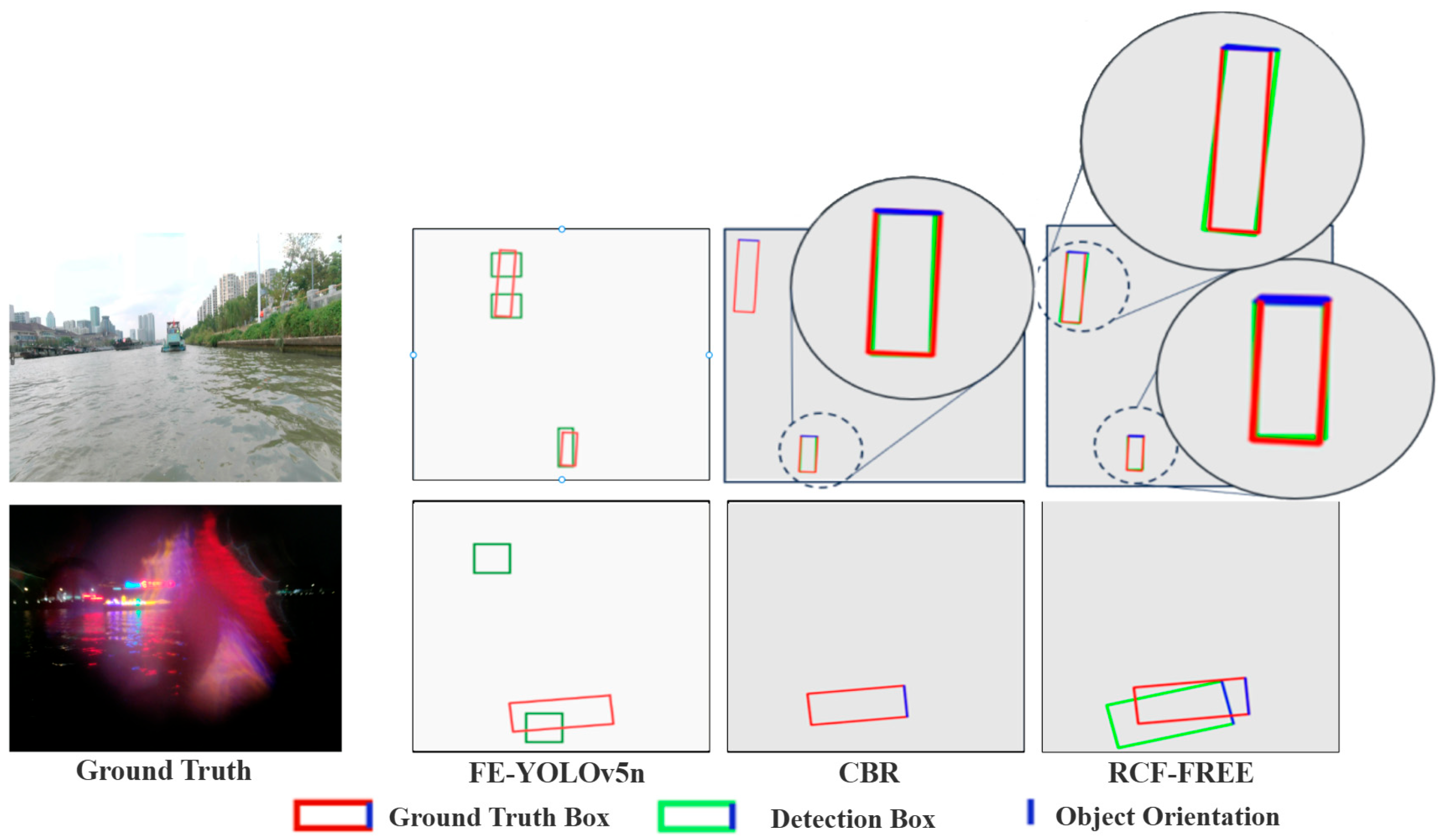
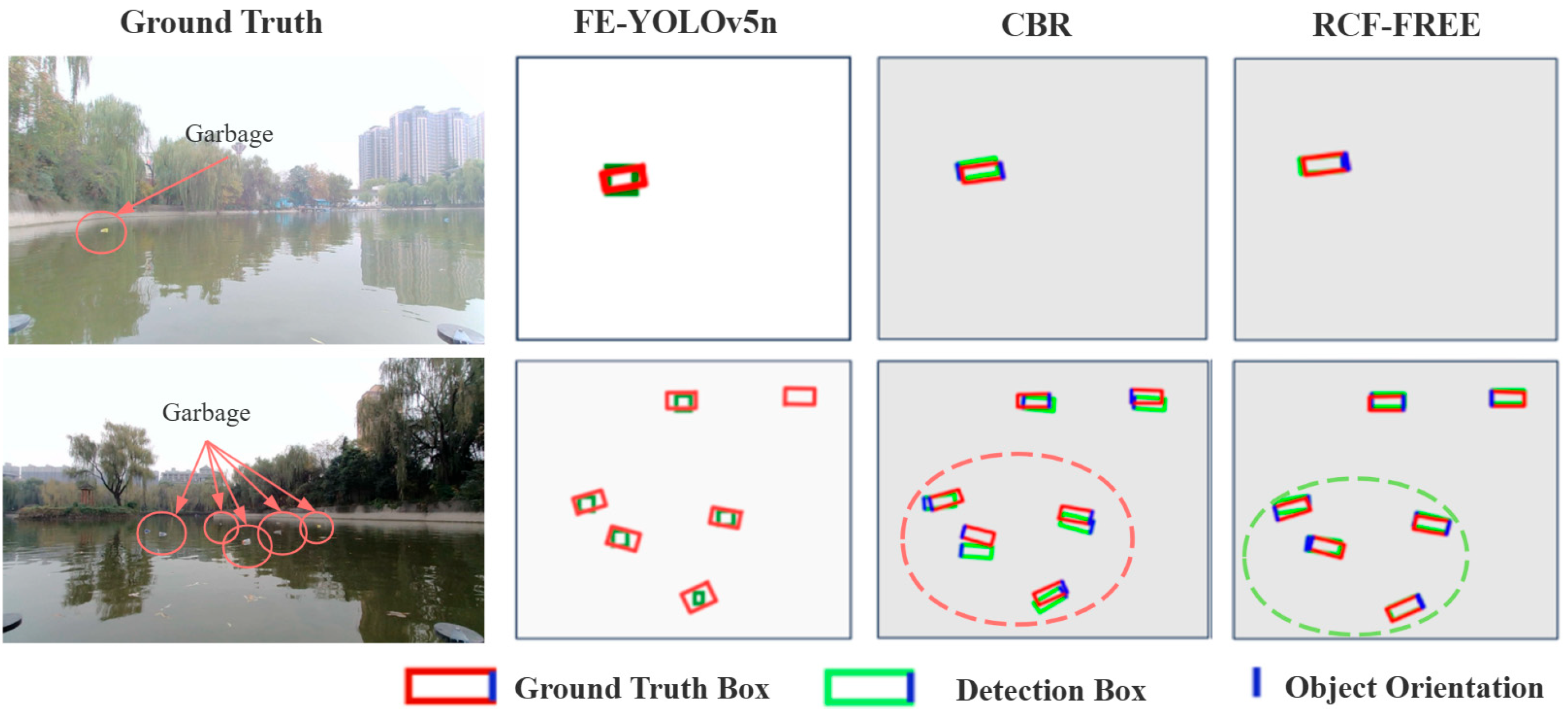
We assess the detection performance in aquatic environments through qualitative comparisons on four distinct scenes from the FloW-BEV and WaterScenes-BEV datasets, covering both floating objects and vessels. Figure 8 presents the perception results for floating objects. The detection boxes from CBR and RCF-Free align more closely with the ground truth than the point cloud clusters produced by the decision-level fusion method FE-YOLOv5s. This demonstrates the feasibility and effectiveness of adapting strategies from autonomous driving for aquatic floating object detection.

In Scenes 1 and 2, RCF-Free produces detection boxes that fit the ground truth more accurately than CBR. This gain in precision stems from our novel point cloud fusion architecture, which yields richer and more precise BEV feature representations. Additionally, the Mobile Self-Attention Module (MAM) refines the front-view features, enhancing the model’s capacity to capture spatially correlated details in challenging water surface conditions. Together, these components enable higher precision in 3D perception of floating objects.

The detection results for two vessel scenes are shown in Figure 9, with detailed enlargements provided for areas of close alignment. Unlike the sparse and fragmented point cloud clusters generated by FE-YOLOv5s for large objects with non-uniform point clouds, both CBR and RCF-Free produce higher-quality BEV detection boxes in an end-to-end manner. However, the vision-only CBR method exhibits missed detections in both scenes. In contrast, RCF-Free successfully detects all objects by effectively leveraging point cloud information through its dedicated feature encoder and multimodal fusion architecture, complemented by enhanced front-view features. This demonstrates its capability for reliable 3D perception of waterborne vessels, laying a solid perceptual foundation for automated navigation akin to autonomous driving. Furthermore, as highlighted by the red and blue circles in Figure 9, RCF-Free achieves more accurate target positioning than the CBR baseline. This underscores the contribution of point cloud data in improving localization accuracy, particularly for small targets, and validates the efficacy of the Triple-Path Cross-View Fusion module in integrating point cloud features with the decoupled front-view and BEV image features.

4.4.2. Qualitative Results on DAIR-V2X-I

We also evaluate the detection performance on the autonomous driving dataset DAIR-V2X-I. Figure 10 and Figure 11 show qualitative results for two representative scenes.

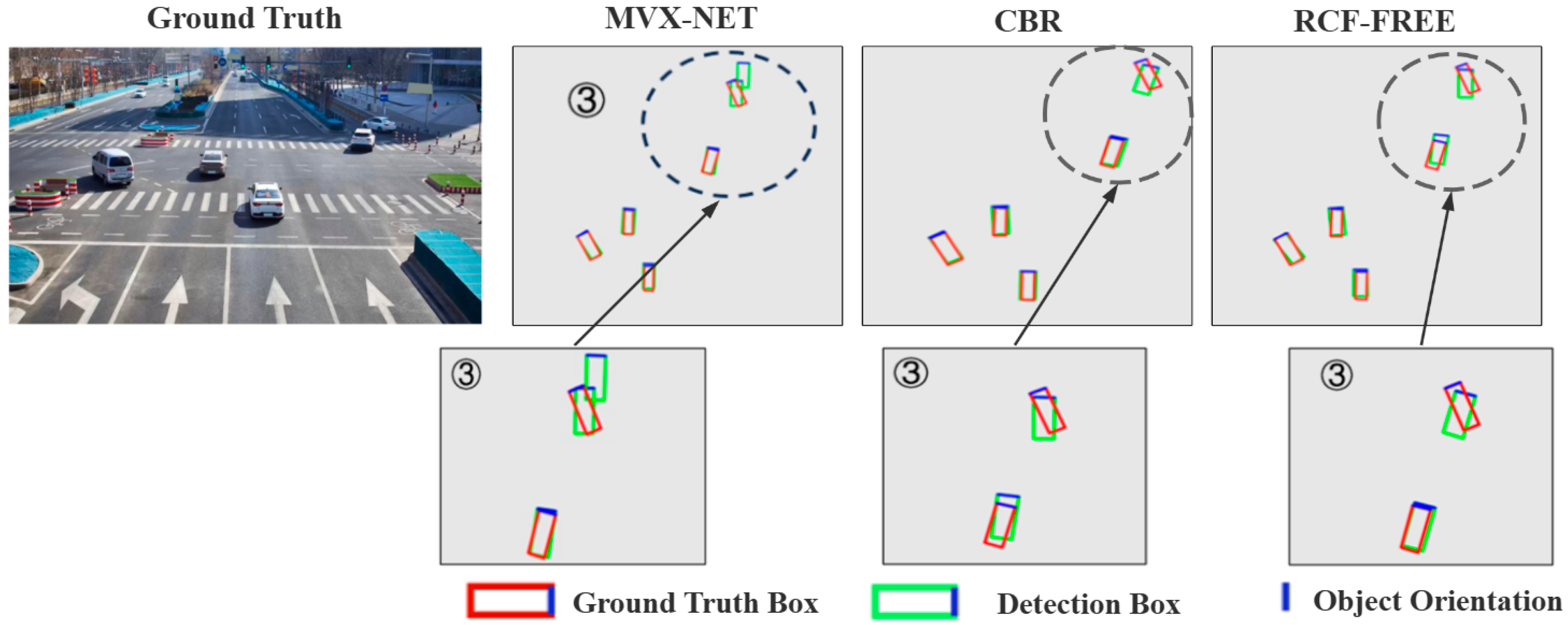
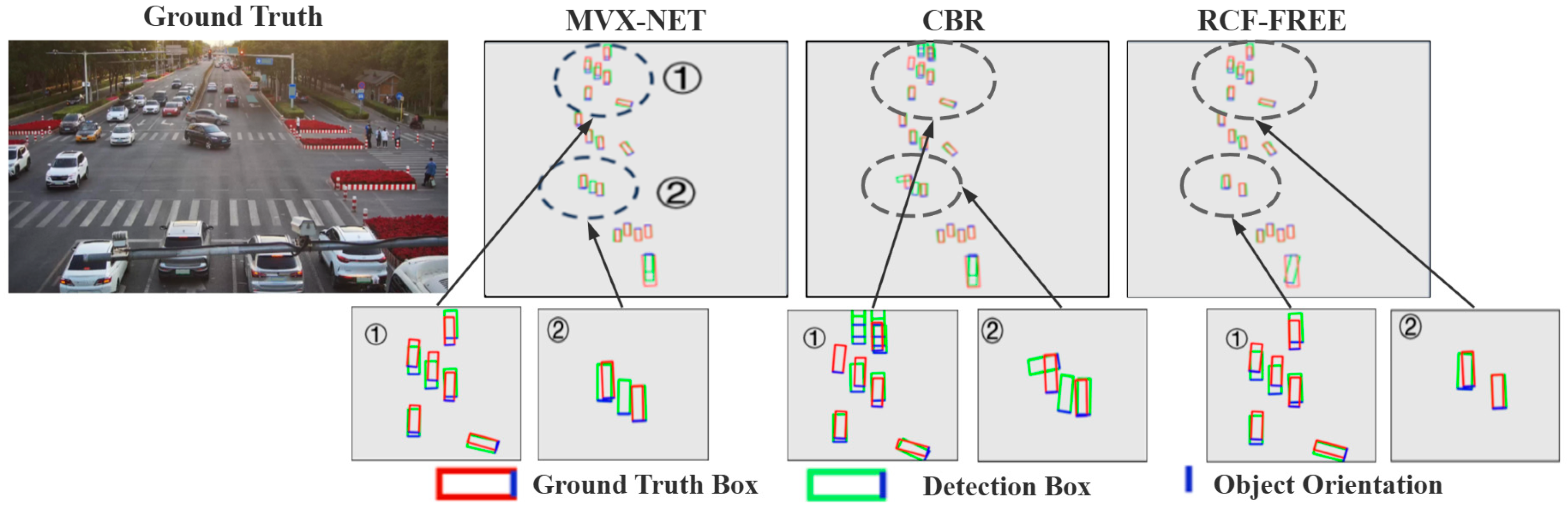
For Scene 1 (Figure 10), we examine two enlarged regions. In Region 1, under high vehicle density, both RCF-Free and the calibration-dependent multimodal method MVX-Net perform robustly, whereas the vision-only CBR shows significant deviations and misses. In Region 2, RCF-Free maintains accurate detections where both MVX-Net and CBR fail, confirming its precision in complex conditions.

In Scene 2 (Figure 11, Region 3), MVX-Net generates a false detection due to point cloud noise, and CBR mislocates a vehicle in the lower-left area, constrained by the limitations of visual sensing. RCF-Free, in comparison, produces more accurate BEV boxes, demonstrating robustness and adaptability across diverse scenarios.

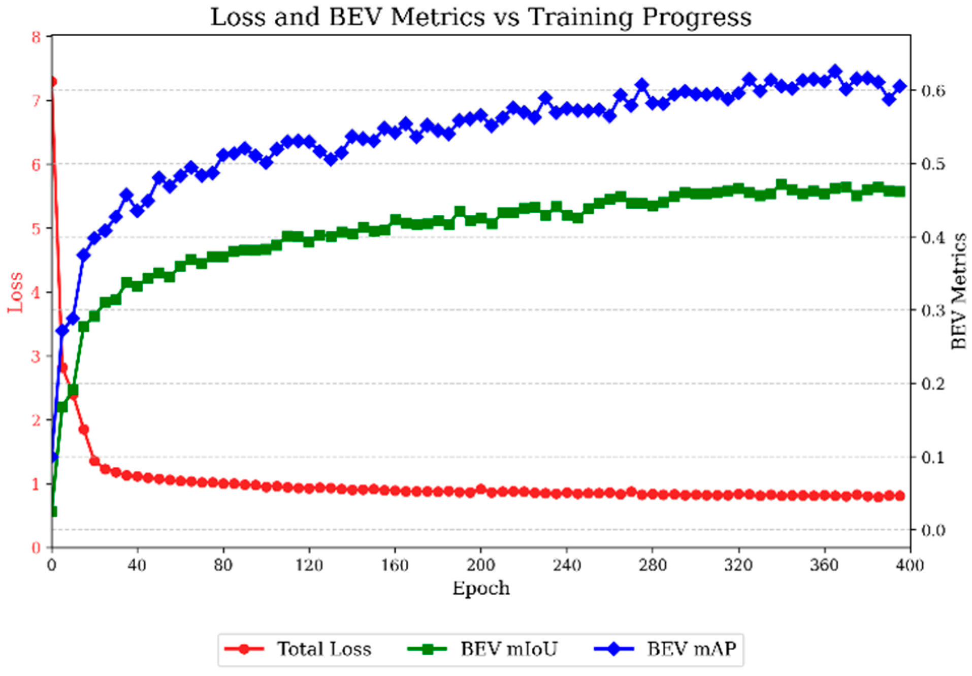
Model convergence: Figure 12 shows the comparison curve between loss and evaluation metrics. In the early stages of training, the model quickly converges. After 40 epochs, the map reaches over 40% and the convergence speed decreases. This continues until the end of training and the optimal result is between 360 and 380 epochs.

4.4.3. Limitation Analysis

To comprehensively assess the performance boundaries of the RCF-Free algorithm, this section discusses the model’s performance in several challenging scenarios based on the test set. This analysis reveals the current limitations of the model and points to directions for future work.

(1)

Insufficient Bounding Box Regression Accuracy in Dense Small-Object Scenes

While RCF-Free demonstrates robust recall for small objects with fewer instances of severe missed detections, its bounding box regression accuracy, particularly for object orientation (yaw), is notably compromised in scenes with densely arranged or closely spaced targets. As shown in Figure 13, when multiple small targets are close to each other in the BEV plane, the algorithm can roughly localize the group but often produces significant errors in estimating individual bounding boxes, especially their orientations. We attribute this primarily to two interrelated factors: First, the inherent sparsity of millimeter-wave radar point clouds limits the geometric cues available for precise contour and orientation estimation. Second, a limitation arises from the training supervision itself. The regression of the front-view (FV) and BEV features is supervised by masks generated from the 3D bounding box labels. In dense small-object scenes, the 2D projections of these 3D boxes onto the FV and BEV planes often result in overlapping or adjacent masks. This causes the supervision signal for individual targets within a cluster to be weakened or ambiguous during training, leading to the orientation inaccuracies observed at inference time.

(2)

Performance Trade-off in Sensor Failure/Degradation Scenarios

The core strength of the algorithm lies in multimodal complementarity. However, when one modality completely fails, its design introduces a specific performance cost. To simulate the extreme case of complete radar sensor failure, we conducted an “empty point cloud input” experiment, where the input to the point cloud branch was set to zero. The results, presented in

Table 8. Algorithm performance with empty point cloud input (FloW-BEV dataset).

Methods	$\mathbf{m}\mathbf{A}{\mathbf{P}}_{\mathbf{B}\mathbf{E}\mathbf{V}}$/%	mIOU/%
CBR	56.9	45.0
RCF-Free	60.5	47.2
RCF-Free (only camera)	55.2	43.6

, show that RCF-Free (only camera) achieves significantly lower performance than the vision-only baseline CBR.

This phenomenon reveals a design trade-off: even with empty point cloud input, the BEV-Point encoder still outputs a rasterized feature map representing “background.” This feature is processed and attempted to be fused in the subsequent Triple-Path Cross-View Fusion module. Although the network may learn to down-weight it, the very process of introducing and fusing this “invalid” feature can interfere with the vision-dominated reasoning pipeline, leading to performance slightly inferior to the CBR baseline optimized specifically for the vision-only task. From another perspective, however, this result conversely proves that effective point cloud features are crucial to the algorithm’s performance gain under normal operation. The performance improvement of RCF-Free (3.4% gain over CBR) does not stem from simple feature stacking but relies on high-quality cross-modal information interaction.

5. Conclusions

In this paper, we introduced RCF-Free, a novel weak calibration multimodal 3D object detection framework for USVs. Our method incorporates three key components: a Mobile Self-Attention Module that enhances the spatial contextual understanding of image features; a BEV-Point feature encoder that effectively represents sparse point clouds in BEV space; and a Triple-Path Cross-View Fusion module that achieves high-quality multimodal feature integration, inspired by techniques from autonomous driving, based on similarity. This architecture ultimately generates high-precision BEV bounding boxes for detected objects. Furthermore, due to the lack of comprehensively annotated 3D multimodal datasets for aquatic environments, we reconstruct and introduce two enhanced datasets—FloW-BEV and WaterScenes-BEV—with full 3D annotations. These datasets fill a critical gap in existing public resources and provide essential data support for training and validating 3D perception algorithms in water surface scenarios.

Experimental results demonstrate that the proposed algorithm outperforms existing methods in both USVs and autonomous driving scenarios, showing significant improvements in aquatic object detection accuracy. RCF-Free effectively addresses common challenges in 3D perception, such as low point cloud quality, inaccurate detection results, while overcoming the dependency on precise calibration. We believe that this approach can offer robust 3D perceptual capabilities for intelligent unmanned vessels and holds substantial application potential in the advancement of USVs.

Looking forward, a critical direction is to enhance the deployment efficiency of RCF-Free on resource-constrained edge devices commonly used on USVs, such as embedded AI computing platforms. Future work will explore model compression and acceleration techniques, including but not limited to knowledge distillation, quantization, and neural architecture search, to significantly reduce the model’s parameter count and computational latency while preserving its accuracy and robustness. This optimization will be essential for achieving real-time, low-power 3D perception in practical, large-scale USV deployments.

References

1. Sun, T.; Guo, R.; Chen, G.; Wang, H.; Li, E.; Zhang, W. RID-LIO: Robust and Accurate Intensity-Assisted LiDAR-Based SLAM for Degenerated Environments. Meas. Sci. Technol. 2025, 36, 36313. [Google Scholar] [CrossRef]
2. Cheng, Q.; Chen, W.; Wang, J.; Mi, X.; Yang, Y.; Sun, R. Multi-Constellation Instantaneous Single Difference Triple-Carrier Ambiguity Resolution in Urban Environments. GPS Solut. 2025, 29, 186. [Google Scholar] [CrossRef]
3. Sun, R.; Sheng, Q.; Cheng, Q.; Shang, X.; Ochieng, W.Y. 3-D Grid-Based Resilient Pseudorange Error Prediction for Adaptive GNSS/IMU Integrated Navigation in Urban Areas. IEEE Internet Things J. 2025, 12, 19264–19279. [Google Scholar] [CrossRef]
4. Wang, X.; Song, X.; Du, L. Review and application of unmanned surface vehicle in China. In Proceedings of the 5th International Conference on Transportation Information and Safety, Liverpool, UK, 14–17 July 2019; pp. 1476–1481. [Google Scholar] [CrossRef]
5. Li, D.; Zhang, F.; Rong, W.; Yue, C.; Zhang, Y.; Liang, Y.; Ren, J. Robust Localization Algorithm for Micromanipulation Targets Under Complex Interference Conditions. IEEE Trans. Autom. Sci. Eng. 2025, 22, 23959–23969. [Google Scholar] [CrossRef]
6. Cheng, Y.; Zhu, J.; Jiang, M.; Fu, J.; Pang, C.; Wang, P.; Sankaran, K.; Onabola, O.; Liu, Y.; Liu, D.; et al. FloW: A dataset and benchmark for floating waste detection in Inland Waters. In Proceedings of the IEEE/CVF International Conference on Computer Vision (ICCV), Montreal, QC, Canada, 11–17 October 2021; pp. 10953–10962. [Google Scholar] [CrossRef]
7. Zhang, L.; Wei, Z.; Shao, Y.; Chen, Z.; Luo, Z.; Dou, Y. A context feature enhancement and adaptive weighted fusion network for river floating debris detection. Eng. Appl. Artif. Intell. 2025, 144, 110095. [Google Scholar] [CrossRef]
8. Lu, M.; Xiao, X.; Zhang, X.; Yang, Y. An accurate inland water garbage recognition network for USV camera images. Meas. Sci. Technol. 2025, 36, 045801. [Google Scholar] [CrossRef]
9. Chen, Y.; Leng, Y.; Zhang, Y. An obstacle detection method for LIDAR after removing water surface clutter. In Proceedings of the 5th International Conference on Computer, Information Science and Artificial Intelligence, Changchun, China, 23–25 September 2022; Volume 12566, pp. 711–721. [Google Scholar] [CrossRef]
10. Liu, J.; Li, H.; Liu, J.; Xie, S.; Luo, J. Real-time monocular obstacle detection based on horizon line and saliency estimation for unmanned surface vehicles. Mob. Netw. Appl. 2021, 26, 1372–1385. [Google Scholar] [CrossRef]
11. Zhou, Z.; Li, Y.; Cao, J.; Zhao, W.; Di, S.; Ailaterini, M. Research on water surface object detection algorithm based on 3D LiDAR. Laser Optoelectron. Prog. 2022, 59, 1815006. [Google Scholar] [CrossRef]
12. Wan, W.; Zeng, T.; Zhang, T.; Li, Y.; Liu, H.; Sun, J. Rapid extraction of nearshore objects. J. Harbin Eng. Univ. 2012, 33, 1158–1163. [Google Scholar]
13. Wang, J.; Zhao, H. Improved YOLOv8 algorithm for water surface object detection. Sensors 2024, 24, 5059. [Google Scholar] [CrossRef]
14. Huang, W.; Feng, H.; Xu, H.; Liu, X.; He, J.; Gan, L.; Wang, X.; Wang, S. Surface vessels detection and tracking method and datasets with multi-source data fusion in real-world complex scenarios. Sensors 2025, 25, 2179. [Google Scholar] [CrossRef]
15. Jiang, W.; Yang, L.; Bu, Y. Research on the Identification and Classification of Marine Debris Based on Improved YOLOv8. J. Mar. Sci. Eng. 2024, 12, 1748. [Google Scholar] [CrossRef]
16. Gu, Q.; Deng, B.; He, Y.; Zhang, Y.; Cheng, L.; Wang, Y. MarineSeg: A CNN–Transformer Hybrid Architecture with Feature Voting Decoder for Robust Semantic Segmentation in USV-Captured Images. Neurocomputing 2026, 671, 132597. [Google Scholar] [CrossRef]
17. Yang, M.; Wang, Z.; Wang, Y.; Wang, S. Resilience-Based Lifetime Performance Assurance Design of Unmanned Underwater Vehicles. J. Mech. Des. 2026, 148, 1–19. [Google Scholar] [CrossRef]
18. Zhang, X.; Pan, H.; Ling, K. Enhanced Robust Association for Multi-Object Tracking in Multibeam Forward-Looking Sonar Video. Ocean Eng. 2026, 350, 124141. [Google Scholar] [CrossRef]
19. Zhou, L.; Gao, J.; Xu, S.; Bai, X. A Numerical Method to Simulate Ice Drift Reversal for Moored Ships in Level Ice. Cold Reg. Sci. Technol. 2018, 152, 35–47. [Google Scholar] [CrossRef]
20. Guan, R.; Jia, L.; Yao, S.; Yang, F.; Xu, S.; Purwanto, E. WaterVG: Waterway visual grounding based on text-guided vision and mmwave radar. IEEE Trans. Intell. Transp. Syst. 2025, 26, 7275–7291. [Google Scholar] [CrossRef]
21. Zhang, M.; Zhang, Y.; Wang, Y.; Wu, Y. Shipborne sea wave radar object detection method based on improved Mask R-CNN. Adv. Ocean Sci. 2025, in press. Available online: http://kns.cnki.net/kcms/detail/37.1387.P.20240703.1009.002.html (accessed on 8 May 2025).
22. Yu, H.; Shen, Z.; Zhao, M.; Yuan, M.; Liu, J.; Wang, X. Obstacle detection for unmanned ships based on quadtree sector layer value clustering. Sci. Technol. Eng. 2024, 24, 5427–5435. [Google Scholar] [CrossRef]
23. Yu, Y.; Liu, H.; Fu, Y.; Jia, W.; Yu, J.; Yan, Z. Embedding Pose Information for Multiview Vehicle Model Recognition. IEEE Trans. Circuits Syst. Video Technol. 2022, 32, 5467–5480. [Google Scholar] [CrossRef]
24. Wang, L.; Fu, Q.; Zhu, R.; Liu, N.; Shi, H.; Liu, Z.; Li, Y.; Jiang, H. Research on High Precision Localization of Space Target with Multi-Sensor Association. Opt. Lasers Eng. 2025, 184, 108553. [Google Scholar] [CrossRef]
25. Shen, Z.; He, Y.; Du, X.; Yu, J.; Wang, H.; Wang, Y. YCANet: Target Detection for Complex Traffic Scenes Based on Camera-LiDAR Fusion. IEEE Sens. J. 2024, 24, 8379–8389. [Google Scholar] [CrossRef]
26. Ren, Y.; Wang, L.; Li, M.; Jiang, H.; Cui, Z.; Yang, M.; Yu, H.; Yang, D. RM2Occ: Re-Projection Multi-Task Multi-Sensor Fusion for Autonomous Driving 3D Object Detection and Occupancy Perception. IEEE Trans. Intell. Transp. Syst. 2025, 26, 20864–20881. [Google Scholar] [CrossRef]
27. Li, R.; Wang, Y.; Sun, S.; Zhang, Y.; Ding, F.; Gao, H. UE-Extractor: A Grid-to-Point Ground Extraction Framework for Unstructured Environments Using Adaptive Grid Projection. IEEE Robot. Autom. Lett. 2025, 10, 5991–5998. [Google Scholar] [CrossRef]
28. Wang, Q.; Tan, R.X.; Feng, Y.Y.; Li, Z.H.; Zhang, H.; Liu, G.Q. A Camera-LiDAR Joint Calibration Method Based on 3D Calibration Target. J. Chin. Inert. Technol. 2023, 31, 100–106. [Google Scholar] [CrossRef]
29. Taylor, Z.; Nieto, J. Motion-Based Calibration of Multimodal Sensor Arrays. In Proceedings of the 2015 IEEE International Conference on Robotics and Automation (ICRA), Seattle, WA, USA, 26–30 May 2015; pp. 4843–4850. [Google Scholar] [CrossRef]
30. Wang, H.; Liu, Y.; Zhao, C.; He, J.; Ding, W.; Chen, X.; Zhou, Z. CaliFormer: Leveraging Unlabeled Measurements to Calibrate Sensors with Self-Supervised Learning. In Proceedings of the 2023 ACM International Joint Conference on Pervasive and Ubiquitous Computing & the 2023 ACM International Symposium on Wearable Computing, Cancún, Mexico, 8–12 October 2023; pp. 743–748. [Google Scholar] [CrossRef]
31. Shi, P.T.; Wei, K.L.; Wu, H.; Li, J.; Zhang, Y.; Chen, X. Extrinsic Calibration Method for LiDAR and Camera Based on Semantic Segmentation in Autonomous Driving Environment. Laser Optoelectron. Prog. 2024, 61, 306–311. [Google Scholar] [CrossRef]
32. Philion, J.; Fidler, S.; Bischof, H.; Frahm, J.-M.; Brox, T.; Vedaldi, A. Lift, Splat, Shoot: Encoding Images from Arbitrary Camera Rigs by Implicitly Unprojecting to 3D. In Computer Vision—ECCV 2020; Lecture Notes in Computer Science; Springer International Publishing AG: Cham, Switzerland, 2020; Volume 12359, pp. 194–210. [Google Scholar] [CrossRef]
33. Liu, Z.; Tang, H.; Amini, A.; Yang, X.; Mao, H.; Rus, D.L.; Han, S. BEVDepth: Acquisition of reliable depth for multi-view 3D object detection. In Proceedings of the AAAI Conference on Artificial Intelligence, Washington, DC, USA, 7–14 February 2023; Volume 37, pp. 1477–1485. [Google Scholar] [CrossRef]
34. Liu, Z.; Tang, H.; Amini, A.; Yang, X.; Mao, H.; Rus, D.L.; Han, S. BEVFusion: Multi-Task Multi-Sensor Fusion with Unified Bird’s-Eye View Representation. In Proceedings of the 2023 IEEE International Conference on Robotics and Automation (ICRA), London, UK, 29 May–2 June 2023; pp. 2774–2781. [Google Scholar] [CrossRef]
35. Stanislas, L.; Dunbabin, M. Multimodal sensor fusion for robust obstacle detection and classification in the maritime RobotX challenge. IEEE J. Ocean Eng. 2018, 44, 343–351. [Google Scholar] [CrossRef]
36. Wu, Y.; Qin, H.; Liu, T.; Liu, H.; Wei, Z. A 3D object detection based on multi-modality sensors of USV. Appl. Sci. 2019, 9, 535. [Google Scholar] [CrossRef]
37. Proença, P.F.; Simões, P. TACO: Trash annotations in context for litter detection. arXiv 2020, arXiv:2003.06975. [Google Scholar] [CrossRef]
38. Yang, M.; Thung, G. Classification of Trash for Recyclability Status; Technical Report; Stanford University: Stanford, CA, USA, 2016. [Google Scholar]
39. Wang, J.; Guo, W.; Pan, T.; Yu, H.; Duan, L.; Yang, W. Bottle detection in the wild using low-altitude unmanned aerial vehicles. In Proceedings of the 21st International Conference on Information Fusion, Cambridge, UK, 10–13 July 2018; pp. 439–444. [Google Scholar] [CrossRef]
40. Li, Y.; Wang, R.; Gao, D.; Liu, Z. A floating-waste-detection method for unmanned surface vehicle based on feature fusion and enhancement. J. Mar. Sci. Eng. 2023, 11, 2234. [Google Scholar] [CrossRef]
41. Yao, R.; Guan, Z.; Wu, Z.; Yue, Y.; Zhu, X.; Ma, J.; Man, K.L.; Seo, H.; Lim, E.G.; Ding, W.; et al. WaterScenes: A multi-task 4D radar-camera fusion dataset and benchmarks for autonomous driving on water surfaces. IEEE Trans. Intell. Transp. Syst. 2024, 25, 16584–16598. [Google Scholar] [CrossRef]
42. Almujally, N.A.; Rafique, A.A.; Al Mudawi, N.; Alazeb, A.; Alonazi, M.; Al-garni, A.; Jalal, A.; Liu, H. Multi-Modal Remote Perception Learning for Object Sensory Data. Front. Neurorobot. 2024, 18, 1427786. [Google Scholar] [CrossRef] [PubMed]
43. Vaswani, A.; Shazeer, N.; Parmar, N.; Uszkoreit, J.; Jones, L.; Gomez, A.N.; Kaiser, Ł.; Polosukhin, I. Attention is all you need. Adv. Neural Inf. Process. Syst. 2017, 30, 5998–6008. [Google Scholar]
44. Mehta, S.; Rastegari, M. Separable self-attention for mobile vision transformers. arXiv 2022, arXiv:2206.02680. [Google Scholar] [CrossRef]
45. Yang, W.; Li, Q.; Liu, W.; Yu, Y.; Ma, Y.; He, S.; Pan, J. Projecting your view attentively: Monocular road scene layout estimation via cross-view transformation. In Proceedings of the IEEE/CVF Conference on Computer Vision and Pattern Recognition (CVPR), Nashville, TN, USA, 20–25 June 2021; pp. 15536–15545. [Google Scholar] [CrossRef]
46. Fan, S.; Wang, Z.; Huo, X.; Wang, Y.; Liu, J. BEV representation for infrastructure perception. In Proceedings of the IEEE/RSJ International Conference on Intelligent Robots and Systems (IROS), Detroit, MI, USA, 1–5 October 2023; pp. 9008–9013. [Google Scholar] [CrossRef]
47. Shi, S.; Guo, C.; Jiang, L.; Wang, Z.; Shi, J.; Wang, X.; Li, H. PV-RCNN: Point-voxel feature set abstraction for 3D object detection. In Proceedings of the IEEE/CVF Conference on Computer Vision and Pattern Recognition (CVPR), Seattle, WA, USA, 14–19 June 2020; pp. 10529–10538. [Google Scholar] [CrossRef]
48. Yu, H.; Luo, Y.; Shu, M.; Huo, Y.; Yang, Z.; Shi, Y.; Guo, Z.; Li, H.; Hu, X.; Yuan, J.; et al. DAIR-V2X: A large-scale dataset for vehicle-infrastructure cooperative 3D object detection. In Proceedings of the IEEE/CVF Conference on Computer Vision and Pattern Recognition (CVPR), New Orleans, LA, USA, 19–24 June 2022; pp. 21361–21370. [Google Scholar] [CrossRef]
49. Gu, X. Research on Key Technologies for Surface Object Perception of Intelligent Unmanned Ships. Master’s Thesis, Guangxi University, Nanning, China, 2023. [Google Scholar]
50. Lang, A.H.; Vora, S.; Caesar, H.; Zhou, L.; Yang, L.; Beijbom, O. PointPillars: Fast encoders for object detection from point clouds. In Proceedings of the IEEE/CVF Conference on Computer Vision and Pattern Recognition (CVPR), Long Beach, CA, USA, 16–20 June 2019; pp. 12697–12705. [Google Scholar] [CrossRef]
51. Li, Z.; Wang, W.; Li, H.; Xie, E.; Sima, C.; Lu, T.; Yu, Q.; Dai, J. BEVFormer: Learning bird’s-eye-view representation from LiDAR-camera via spatiotemporal transformers. IEEE Trans. Pattern Anal. Mach. Intell. 2024, 47, 2020–2036. [Google Scholar] [CrossRef]
52. Yan, Y.; Mao, Y.; Li, B. SECOND: Sparsely embedded convolutional detection. Sensors 2018, 18, 3337. [Google Scholar] [CrossRef]
53. Meyer, M.; Kuschk, G.; Tomforde, S. Graph convolutional networks for 3D object detection on radar data. In Proceedings of the IEEE/CVF International Conference on Computer Vision (ICCV), Montreal, QC, Canada, 11–17 October 2021; pp. 3060–3069. [Google Scholar] [CrossRef]
54. Rukhovich, D.; Vorontsova, A.; Konushin, A. ImVoxelNet: Image to voxels projection for monocular and multi-view general-purpose 3D object detection. In Proceedings of the IEEE/CVF Winter Conference on Applications of Computer Vision (WACV), Waikoloa, HI, USA, 3–8 January 2022; pp. 2397–2406. [Google Scholar] [CrossRef]
55. Yang, L.; Yu, K.; Tang, T.; Li, J.; Yuan, K.; Wang, L.; Zhang, X.; Chen, P. BEVHeight: A robust framework for vision-based roadside 3D object detection. In Proceedings of the IEEE/CVF Conference on Computer Vision and Pattern Recognition (CVPR), Vancouver, BC, Canada, 18–22 June 2023; pp. 21611–21620. [Google Scholar] [CrossRef]
56. Wang, W.; Wang, Y.; Lu, G.; Zheng, S.; Zhan, X.; Ye, Z.; Tan, J.; Wang, G.; Wang, X.; Li, B. Bevspread: Spread voxel pooling for bird’s-eye-view representation in vision-based roadside 3D object detection. In Proceedings of the IEEE/CVF Conference on Computer Vision and Pattern Recognition, Seattle, WA, USA, 17–21 June 2024; pp. 14718–14727. [Google Scholar] [CrossRef]
57. NVIDIA-AI-IOT. CUDA-V2XFusion, 2024. Available online: https://github.com/NVIDIA-AI-IOT/Lidar_AI_Solution/tree/master/CUDA-V2XFusion (accessed on 5 November 2024).
58. Xu, J.; Song, C.; Shi, C.; Liu, H.; Wang, Q. UncertainBEV: Uncertainty-Aware BEV Fusion for Roadside 3D Object Detection. Image Vis. Comput. 2025, 159, 105567. [Google Scholar] [CrossRef]
Figure 1. The Overall Architecture of the RCF-Free Algorithm ((a) BEV point cloud feature encoder, (b) Mobile Self-Attention Module (MAM), and (c) Triple-Cross Fusion Module; * means element-wise multiplication).
Jmse 14 00867 g001
Figure 2. The Orthogonal Relationship between the Front-view Features and the BEV Features.
Jmse 14 00867 g002
Figure 3. Example images of FloW-BEV dataset.
Jmse 14 00867 g003
Figure 4. Millimeter-wave Point Cloud of the FloW-BEV Dataset.
Jmse 14 00867 g004
Figure 5. Partial Samples of the WaterScenes-BEV Dataset.
Jmse 14 00867 g005
Figure 6. Millimeter-Wave Point Cloud of the WaterScenes-BEV Dataset.
Jmse 14 00867 g006
Figure 7. Using the LabelCloud Tool to Annotate the Point Cloud Bounding Box in the BEV Perspective for Floating Objects on the Water Surface.
Jmse 14 00867 g007
Figure 8. Comparison of the Detection Results on FloW-RI.
Jmse 14 00867 g008
Figure 9. Comparison of Detection Results on WaterScenes-BEV.
Jmse 14 00867 g009
Figure 10. Comparison of the Detection Results of the Algorithm on DAIR-V2X-I (Scene 1).
Jmse 14 00867 g010
Figure 11. Comparison of the Detection Results of the Algorithm on DAIR-V2X-I (Scene 2).
Jmse 14 00867 g011
Figure 12. Loss convergence curve and Comparison between LOSS and metrics.
Jmse 14 00867 g012
Figure 13. Examples of FV and Bev labels in dense areas on the Flow-BEV dataset and Dair-V2X dataset (In the test results on Flow-BEV dataset, the red box is ground truth, the green is the prediction box, and the red point is the target center point).
Jmse 14 00867 g013