Unified Stochastic Differential Equation Modeling and Fuzzy-RL Control for Turbulent UWOC

Abstract

Underwater wireless optical communication (UWOC) for autonomous underwater vehicles is severely compromised by the coupling of oceanic optical turbulence and platform motion. Traditional static statistical models fail to capture the temporal evolution of these stochastic processes, hindering effective real-time beam tracking. This paper proposes a unified dynamic framework and a hybrid intelligent control strategy to address beam misalignment in turbulent environments. First, a physically motivated stochastic differential equation (SDE) model is derived from the Radiative Transfer Equation via diffusion approximation. Validated by an inverse Fokker–Planck approach, this model accurately reconstructs drift fields for diverse channel conditions, serving as a dynamic generator for time-varying fading. Second, to maintain robust link alignment, a hybrid Fuzzy-Reinforcement Learning control strategy is developed. This approach integrates the interpretability of fuzzy logic with the adaptive optimization of Q-learning, incorporating a supervisor mechanism to handle deep fading events. Numerical simulations and hardware-in-the-loop (HIL) experiments demonstrate the system’s efficacy. The proposed controller achieves a median alignment error of 3.64 mm and reduces transient errors by over 80% compared to classical PID controllers during signal recovery. These results confirm that the proposed framework significantly enhances link stability and tracking robustness for AUVs in complex random media.

1. Introduction

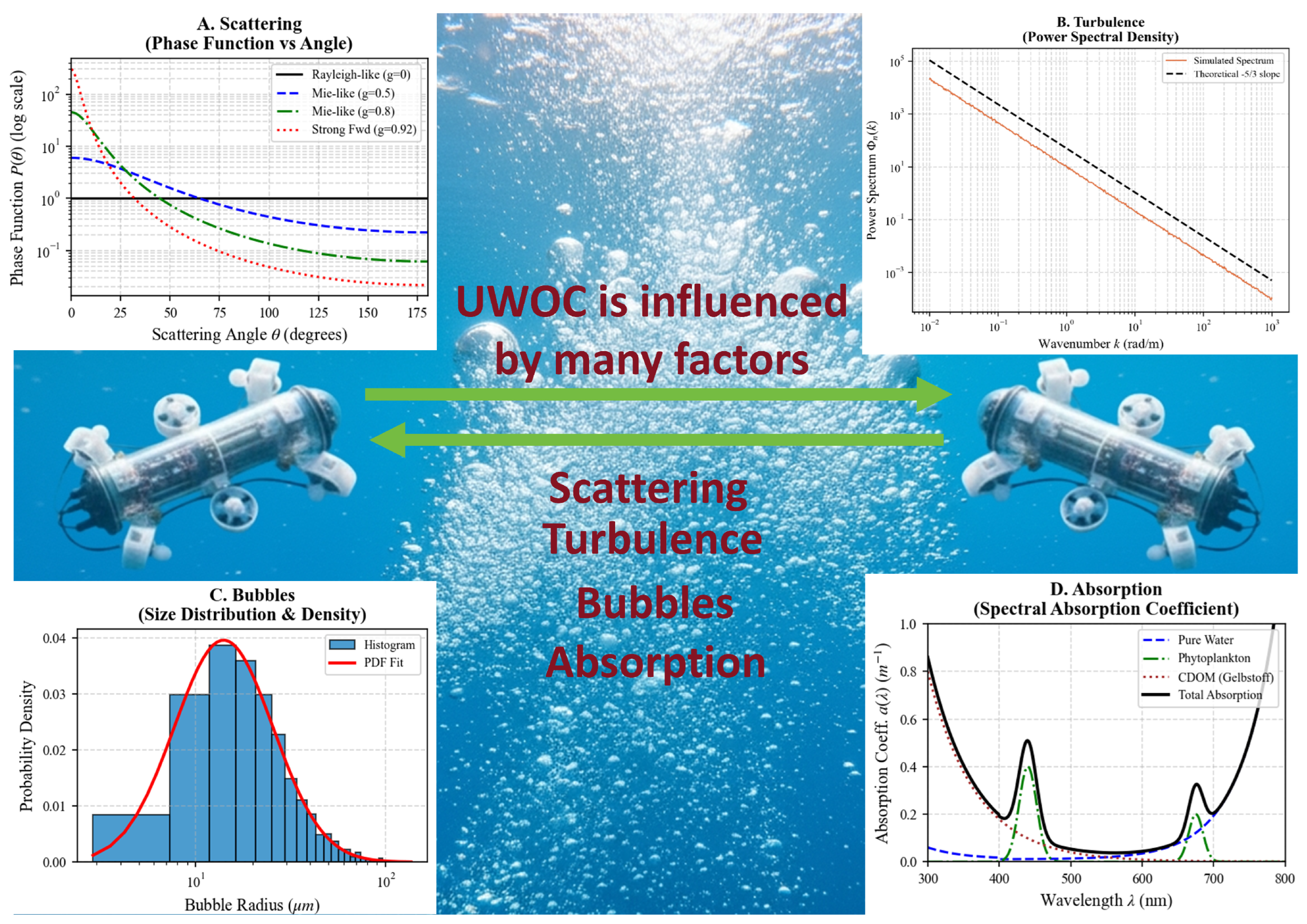
The propagation of optical waves in complex underwater environments is a fundamental problem in the physics of random media, governed by highly nonlinear interactions between photon streams and turbulent flow dynamics [1,2]. With the expansion of marine exploration, autonomous underwater vehicles (AUVs) have become critical platforms for deep-sea monitoring and resource inspection [3,4]. However, the reliability of high-bandwidth underwater wireless optical communication (UWOC) on these dynamic platforms is severely compromised by the stochastic nature of the channel. The coupling of oceanic optical turbulence—induced by random fluctuations in temperature and salinity [5,6]—with the mechanical jitter of the AUV platform creates a complex stochastic system characterized by intense scintillation and beam misalignment [7,8]. The diverse physical mechanisms governing these impairments—ranging from the scattering phase function and turbulence power spectrum to bubble size distributions and spectral absorption—are visually summarized in Figure 1.

Over the past few decades, significant efforts have been dedicated to the statistical characterization of fading channels. Classical distributions have provided solid foundations for theoretical analysis. For instance, the log-normal distribution was widely adopted to describe weak turbulence regimes. Al-Habash et al. utilized this model to analyze the probability density function (PDF) of irradiance, demonstrating its effectiveness in clear ocean waters [9]. However, experimental data revealed its inadequacy in describing stronger fluctuations. To address this, Gamma–Gamma and Malaga models were proposed for moderate-to-strong turbulence [10,11]. Specifically, recent studies have derived closed-form expressions for error performance based on the Malaga distribution, showing a better fit than log-normal under diverse salinity gradients [12]. More recently, mixture models have been introduced to capture heavy-tailed behaviors. For example, Lou et al. proposed the exponential generalized Gamma (EGG) distribution to characterize air bubble-induced fading [13]. Their simulation results indicated that the EGG model could accurately fit the jagged peaks of irradiance caused by particulate scattering [14]. Despite these achievements, a fundamental limitation remains: most existing works focus on static PDFs. They quantify the equilibrium probability of fading states but fail to describe the temporal evolution and correlation of the underlying stochastic processes. They answer “what is the probability of fading,” but cannot answer “how the channel state evolves continuously over time,” which is critical for the design of real-time tracking systems [15,16]. Additionally, the increasing availability of high-fidelity simulation frameworks for underwater vehicles—including hardware-in-the-loop testbeds and digital-twin–enabled modeling—further highlights the need for dynamic, temporally coherent channel representations suitable for closed-loop autonomy [17,18]. Recent experimental and system-level studies have also revisited UWOC path-loss behavior across different water environments and hybrid air–water visible light links, further emphasizing the importance of environment-dependent channel characterization [19,20].

In the context of mobile AUVs, the channel is not a static random variable but a continuous-time dynamical system driven by environmental noise. Stochastic differential equations (SDEs) offer a powerful mathematical apparatus to model such systems [21,22]. Unlike Monte Carlo ray tracing, which is computationally prohibitive for real-time control [23], SDEs can compactly describe the trajectory of wave propagation in random media as diffusion processes [24,25]. Previous studies have attempted to link physical equations with stochastic models. For instance, Fu et al. explored the diffusion approximation of the Radiative Transfer Equation (RTE) [26], while other works have discussed stochastic radiative transfer in random media [27,28,29]. However, a unified dynamic stochastic framework that can reproduce a broad class of stationary channel statistics and their temporal evolution within a single Langevin-type formulation is still lacking.

Parallel to channel modeling, robust beam alignment control is equally critical. Traditional methods typically rely on PID controllers or active disturbance rejection control (ADRC). While simple, these linear controllers often exhibit performance degradation, such as integral windup under non-Gaussian noise and sudden signal interruptions [30]. Consequently, intelligent control methods have gained attention. Deep Reinforcement Learning (DRL) algorithms, such as Deep Q-Networks and Deep Deterministic Policy Gradient, have been applied to visual serving tasks. For example, ref. [31] utilized DDPG to stabilize an underwater vehicle, demonstrating superior adaptability compared to classical control. However, these DRL methods typically require massive neural networks and substantial computational resources, specifically GPUs, which are often constrained on embedded AUV platforms. Furthermore, the “black-box” nature of neural networks lacks interpretability. In contrast, Fuzzy Reinforcement Learning (Fuzzy-RL) integrates the interpretability of fuzzy logic with the learning capability of Q-learning [32,33]. It offers a lightweight, computationally efficient alternative that is better suited for real-time operation on limited-resource hardware; yet, this approach has rarely been explored in the context of stochastic underwater optical beam tracking.

To address these theoretical and practical gaps, this paper proposes a unified stochastic dynamic framework and a hybrid intelligent control strategy. The main contributions are threefold:

(1)

From Physics to Stochastic Dynamics: Starting from the RTE, a physically motivated SDE representation is derived via diffusion approximation. An inverse Fokker–Planck equation approach is introduced to demonstrate that the proposed SDE acts as a unified stochastic generator for a broad class of stationary channel statistics, with the inverse Fokker–Planck formulation providing a mathematical route for reconstructing drift fields from target stationary PDFs.

(2)

Coupled Nonlinear Modeling: The coupling between AUV attitude dynamics and channel fading is explicitly modeled. Consequently, the beam alignment problem is reformulated as the stabilization of a nonlinear system subjected to multiplicative noise, extending classical wave propagation theories [34] to mobile engineering applications.

(3)

Hybrid Intelligent Control: A lightweight hybrid Fuzzy-RL controller is designed to provide robust adaptive beam-pointing control under the reduced plant model, with mean-square boundedness and asymptotic convergence to a bounded neighborhood established under Assumptions A1–A3 stated in Appendix A.1. By integrating the logical interpretability of fuzzy rules with the adaptive optimization of tabular Q-learning, this strategy effectively mitigates deep fading events with minimal computational overhead compared to deep RL approaches.

2. Materials and Methods

2.1. AUV Platform Model

The AUV state is represented by the vector $x\left(t\right)={\left[x,y,z,\phi ,\psi ,\theta \right]}^T$, which comprises the vehicle position in the inertial coordinate system and the attitude Euler angles. This process is modeled using an SDE:

$$dx\left(t\right)=f\left(x\left(t\right),u\left(t\right)\right)dt+G\left(x\left(t\right)\right)dw\left(t\right)$$

(1)

where $f\left(x,u\right)$ denotes the deterministic drift term, including propulsion input $u\left(t\right)$ and hydrodynamic effects. The diffusion matrix G(x) scales the environmental noise. w(t) is a multidimensional Wiener process representing environmental flow disturbances, and its covariance can be designed to reflect different physical disturbance levels.

External disturbances affect the dynamics of $x\left(t\right)$. Consequently, the AUV requires real-time state updates to maintain UWOC optical alignment. Practical engineering solutions often employ multi-sensor fusion, integrating data from Doppler Velocity Logs (DVLs) and Inertial Measurement Units (IMUs). An Extended Kalman Filter (EKF) is typically adopted for state estimation.

Modern AUVs are generally equipped with attitude control systems to achieve stable hovering or to follow predetermined trajectories. These systems are designed to compensate for external disturbances, including nonlinear hydrodynamic effects as well as drift and attitude variations caused by ocean currents. During actual deployment, ocean currents impose random fluctuations on the AUV. However, after compensation by the control system, these fluctuations do not necessarily propagate to the laser gimbal in their original full-order form.

Explicitly modeling the full six-dimensional Wiener process associated with ocean-current disturbances would lead to excessive computational overhead and a severe curse-of-dimensionality problem. To address the core UWOC challenges of turbulence and scattering under real-time constraints, this study prioritizes engineering practicality. Instead of solving the full hydrodynamic equations online, a stochastic decoupling strategy is adopted, in which complex environmental disturbances are represented as equivalent random processes acting directly on the gimbal base. This approach isolates the dominant high-frequency jitter affecting the optical link while preserving the principal disturbance pathway relevant to beam tracking and control feasibility.

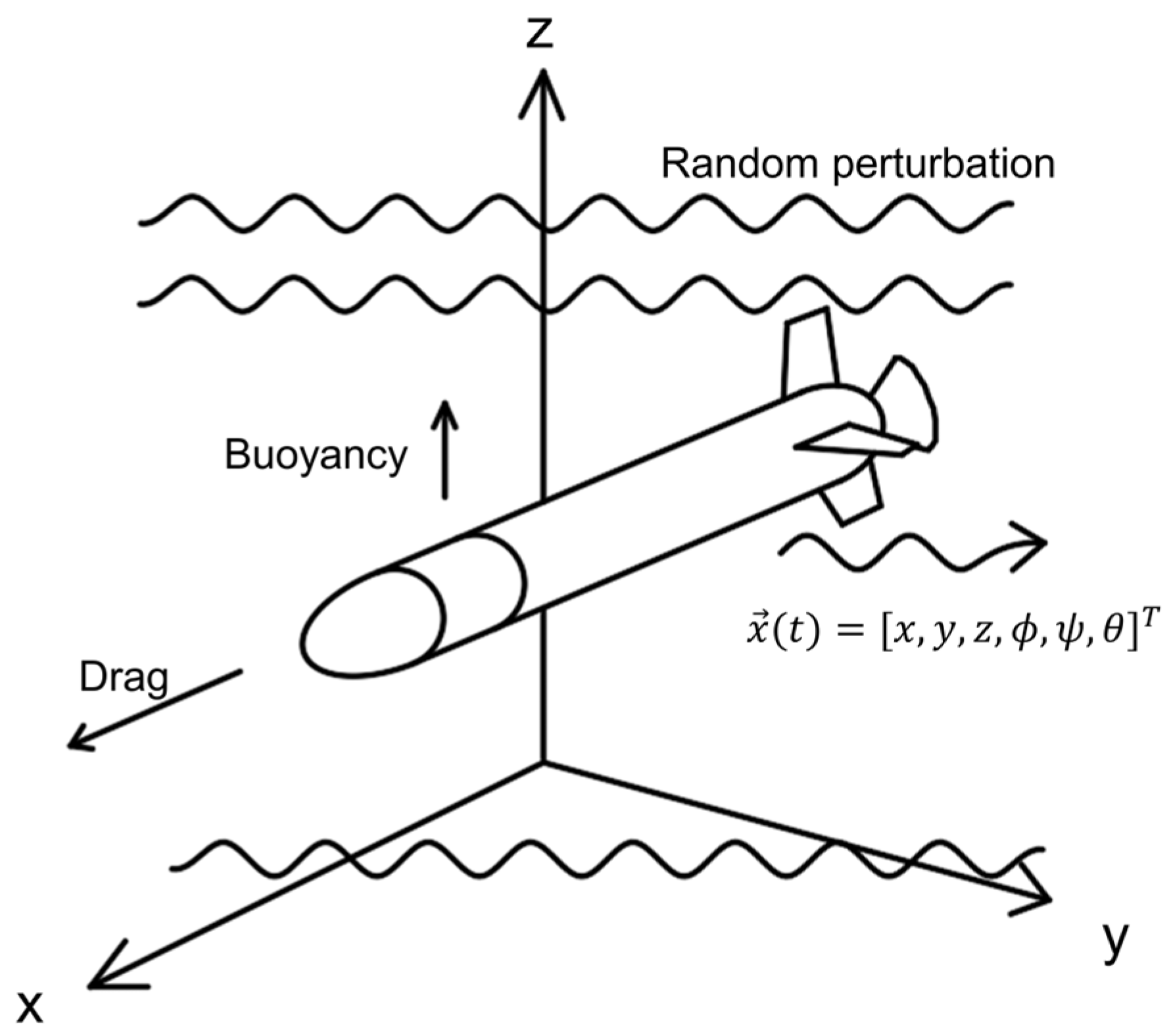
The above decoupling approximation is justified by a timescale-separation argument. In typical UWOC beam-tracking scenarios, the gimbal servo dynamics are substantially faster than the dominant low-frequency AUV attitude variations, allowing the platform motion to be treated as a slowly varying base disturbance. Under this assumption, inertial stabilization and inner-loop attitude compensation suppress most low-frequency vehicle motion, whereas the residual high-frequency jitter remains the dominant factor affecting optical alignment. Accordingly, the reduced model should be interpreted as an engineering abstraction for beam-pointing control rather than as a full hydrodynamic replacement for 6-DOF AUV motion. The resulting kinematic relationship, which illustrates how stochastic perturbations couple with hydrodynamic forces to influence the state vector $x\left(t\right)$, is depicted in Figure 2.

The gimbal is fixed to the AUV. The pointing vector $\theta \left(t\right)={\left[\alpha \left(t\right),\beta \left(t\right)\right]}^T$, defined by azimuth $\alpha$ and elevation $\beta$, is used to decompose the beam pointing angle. Its dynamics are defined as

$$\theta \left(t\right)=Kv\left(t\right)$$

(2)

where $K$ is the servo gain matrix, and $v\left(t\right)$ is the control input. Geometrically, $\theta \left(t\right)$ aligns the beam axis with the receiver. The AUV attitude is coupled to the gimbal via rotation matrices. In turbulent media, beam deflection caused by complex environmental effects requires adaptive adjustment. This is modeled as perturbations to the effective pointing ${\theta }^{*}\left(t\right)$.

2.2. Channel-Pointing Coupling Model

Before establishing the channel-pointing coupling model, it is essential to define the key performance metrics of the underwater optical communication system. This facilitates linking the physical model with communication performance.

The performance of UWOC systems is primarily characterized by three parameters: power transmission gain, directional coupling efficiency, and signal-to-noise ratio.

(1) Power Transmission Gain: Let $P_t$ denote the transmitted power and $P_r\left(t\right)$ denote the received power. The channel gain $G\left(t\right)$ is defined as

$$G\left(t\right)={\displaystyle \frac{P_r\left(t\right)}{P_t}}={\eta }_p\left(t\right)\exp \left[-cd\left(x\left(t\right)\right)\right]$$

(3)

where $c$ is the optical attenuation coefficient of the medium, $d\left(x\left(t\right)\right)$ is the optical propagation distance, and ${\eta }_p\left(t\right)$ represents the directional coupling efficiency caused by beam-angle deviation.

(2) Directional Coupling Efficiency: The geometric overlap between the transmitted beam and the receiving aperture determines the effective power transfer rate of the link. The pointing efficiency can be approximated as

$${\eta }_p\left(t\right)=\exp \left(-{\displaystyle \frac{\Vert \theta \left(t\right)-{\theta }^{*}\left(t\right){\Vert }^2}{2{\sigma }_{\theta }}}\right)$$

(4)

where $\theta \left(t\right)$ represents the current pointing vector, ${\theta }^{*}\left(t\right)$ denotes the optimal pointing direction, and ${\sigma }_{\theta }$ indicates the angular error variance. When beam control precision is high and jitter is low, ${\eta }_p\left(t\right)$ approaches 1. Conversely, as the beam pointing error increases, this value decreases significantly, reflecting link loss.

(3) Signal-to-Noise Ratio (SNR): To establish a physically consistent communication-performance model, we adopt a standard intensity-modulated/direct-detection (IM/DD) receiver framework. The received optical power is first expressed as

$$P_r\left(t\right)=h\left(t\right)P_t$$

(5)

where $h\left(t\right)$ is the effective channel gain. After photodetection, the signal photocurrent becomes

$$i_s\left(t\right)=R{P}_r\left(t\right)$$

(6)

with $R$ (A/W) being the photodetector responsivity.

The electrical SNR, accounting for dominant shot noise and thermal noise, is then written as

$$\mathrm{SNR}\left(t\right)={\displaystyle \frac{{(R{P}_r\left(t\right))}^2}{{\sigma }_{\mathrm{shot}}^2+{\sigma }_{\mathrm{thermal}}^2}}={\displaystyle \frac{{(Rh\left(t\right)P_t)}^2}{2eRB{P}_r\left(t\right)+4k_B{T}_{0}B/R_L}}$$

(7)

where $e$ is the electron charge, $B$ is the receiver’s electrical bandwidth, $k_B$ is Boltzmann’s constant, $T_0$ is the absolute temperature, and $R_L$ is the load resistance.

For OOK modulation with a fixed detection threshold, the instantaneous bit error rate (BER) is approximated by

$$\mathrm{BER}\left(t\right)=Q\left(\sqrt{\mathrm{SNR}\left(t\right)}\right)={\displaystyle \frac{1}{2}}\mathrm{erfc}\left(\sqrt{{\displaystyle \frac{\mathrm{SNR}\left(t\right)}{2}}}\right)$$

(8)

Since $h\left(t\right)$ is affected by the superposition of pointing error and water-body effects, its random fluctuations remain the fundamental cause of the time-varying characteristics of SNR and BER. The average BER can be obtained by taking the expectation over the distribution of $h\left(t\right)$.

The above expressions provide a physically grounded link between the SDE-derived channel gain $h\left(t\right)$ and communication-level performance metrics.

In summary, $h\left(t\right)$ is the core random variable reflecting link-performance fluctuations. Therefore, modeling the dynamic behavior of $h\left(t\right)$ is crucial for describing the statistical characteristics of underwater optical channels.

Channel gain $h\left(t\right)$ fluctuates due to absorption, scattering, and turbulence. The dynamic coupling between channel gain and pointing is first derived, and the SDE framework is then utilized to quantify the propagation of uncertainty. Extending the static Beer–Lambert model, $h\left(t\right)$ is formulated as an SDE.

$$\begin{array}{c}dh\left(t\right)=\mu \left(h\left(t\right),\theta \left(t\right),x\left(t\right)\right)dt+\sigma \left(h\left(t\right),x\left(t\right)\right)dw\left(t\right)\end{array}$$

(9)

Here, the drift term

$$\begin{array}{c}\mu \left(h,\theta ,x\right)=-cd\left(x\right)h+\gamma exp\left(-{\displaystyle \frac{\Vert \theta -{\theta }^{*}{\Vert }^2}{2{\sigma }_{\theta }}}\right)\end{array}$$

(10)

incorporates both absorption-scattering losses and a penalty for pointing misalignment.

The terms are defined as follows:

• $-c\dot{d}\left(x\right)h$: path-loss term based on the Beer–Lambert law.
• $c$: extinction coefficient. This parameter is water-dependent and represents the sum of absorption and scattering. It is measured in ${\mathrm{m}}^{-1}$, with values approximately ranging from 0.1 to 1 ${\mathrm{m}}^{-1}$ in the blue-green wavelength band.
• $d\left(x\right)$ slant range, representing the Euclidean distance between the AUV and the receiver, which varies over time.
• $h$: current gain.
• $\gamma \exp \left(-{\displaystyle \frac{\parallel \theta -{\theta }^{*}{\parallel }^2}{2{\sigma }_{\theta 2}}}\right)$: pointing-recovery term. Here, $\gamma$ is the scaling factor, $\theta \left(t\right)$ is the current gimbal pointing vector, ${\theta }^{*}\left(t\right)$ is the ideal alignment angle, and ${\sigma }_{\theta }$ is the bm-divergence-related angular parameter. This Gaussian penalty function approaches $\gamma$ when $\theta \approx {\theta }^{*}$, and decays exponentially as the pointing deviation increases, thereby simulating power loss due to misalignment.

The diffusion term

$$\begin{array}{c}\sigma \left(h,x\right)dw\left(t\right)\end{array}$$

(11)

captures the random fluctuations in channel gain. In UWOC, these fluctuations are primarily caused by random variations in the underwater refractive index $n\left(z\right)$ due to turbulence, temperature, and salinity gradients.

• $dw\left(t\right)$: increment of the Wiener process.
• $\sigma \left(h,x\right)$: diffusion coefficient. For weak turbulence where the Rytov variance satisfies ${\sigma }_r^2<1$, it can be approximated as

  $${\sigma }^2\left(h,x\right)\propto h^2{k}^2\int d\left(x\right)C_n^2\left(z\right)dz$$

  (12)

This expression is based on the Rytov approximation in optical turbulence theory, where $k=2\pi /\lambda$ is the wave number and $C_n^2\left(z\right)$ is the structural constant of refractive index in a layered medium. Integration along the propagation path represents the accumulation of turbulence intensity. For strong turbulence or scattering, Monte Carlo ray tracing may be used to simulate photon paths and pulse responses, enabling empirical estimation of $\sigma$.

Communication capacity is calculated via

$$C\left(t\right)={\displaystyle \frac{1}{2}}\log \left(1+{\displaystyle \frac{P{h}^2\left(t\right)}{{\sigma }_n^2}}\right)$$

(13)

where $P$ is the transmit power and ${\sigma }_n^2$ is the noise variance. Under random perturbations, $C\left(t\right)$ varies randomly over time. Its expected value $E\left[C\left(t\right)\right]$ must be computed to evaluate average system performance. When analytical solutions are unavailable, this expectation can be approximated using moment closure or Monte Carlo integration.

The alignment error

$$e\left(t\right)=\theta \left(t\right)-{\theta }^{*}\left(t\right)$$

(14)

directly governs BER variation. For OOK modulation, it is approximated through the corresponding $Q$-function of the instantaneous SNR. The optimization objective is therefore to minimize $E\left[e\left(t\right)\right]$ while maximizing $E\left[C\left(t\right)\right]$ within a system governed by SDEs.

The detailed Fokker–Planck formulation and the first- and second-order moment derivations are omitted here for readability and are summarized in Appendix C. Physically, these derivations show that pointing deviation weakens the effective recovery contribution in the drift term, while turbulence-induced diffusion governs the temporal spreading of the channel statistics.

2.3. Parameter Mapping and Statistical Averaging

Although the channel gain SDE model is complete, its high nonlinearity poses computational challenges. To construct a simplified model that retains physical interpretability while enabling statistical identifiability, stochastic averaging theory is employed. This theory processes the slow variables in space and angle, thereby transforming them into calibratable parameters. Specifically, spatial-angular averaging is performed on the drift term $\mu$ and diffusion term $\sigma$ in Equations (10) and (11). Under weak turbulence conditions, their averaged forms can be expressed as

$$\mu \left(I\right)=-aI+b,\sigma \left(I\right)=k{I}^{\gamma /2}$$

(15)

This mapping simplifies the complex space-angle coupling into a low-dimensional parametric form based on stochastic averaging theory while preserving the model’s physical consistency. The resulting equivalent stochastic differential equation is

$$d{I}_t=\left(-a{I}_t+b\right)dt+k{I}_{t\gamma /2}d{W}_t+d{J}_t$$

(16)

The physical interpretation, dimensional consistency, and representative value ranges of the reduced variables and parameters are summarized in

Table 1. Summary of key parameters in the reduced SDE channel model: physical interpretation, SI-consistent units, and representative value ranges under clear-to-coastal water conditions.

Symbol	Physical Interpretation	Unit	Representative Range/Typical Form
$a$	Effective linear attenuation rate, encompassing absorption and out-scattering losses along the propagation path	${\mathrm{s}}^{-1}$	0.10–0.50
$b$	Restoring/compensation coefficient, representing the combined effect of beam re-alignment recovery and equivalent source compensation	${\mathrm{s}}^{-1/2}$ if $I_t$ is normalized; otherwise ${\mathrm{intensity}\mathrm{s}}^{-1}$	0.05–0.30
$k$	Diffusion intensity coefficient, characterizing the strength of turbulence-induced irradiance fluctuations	${\mathrm{s}}^{-1/2}$ if $I_t$ is normalized	0.15–0.65
$\gamma$	State-dependent noise exponent, governing the nonlinear scaling of multiplicative diffusion with respect to the instantaneous channel state	(dimensionless)	1.0–2.0
$I_t$	Reduced stochastic state variable in the averaged SDE; equivalent received optical intensity used for modeling and control	(dimensionless, normalized)	$\left[0,1^{+}\right]$
$h\left(t\right)$	Normalized instantaneous channel gain, defined as the ratio of received optical irradiance/power to the transmit reference level	(dimensionless)	$\left[0,1^{+}\right]$
${\sigma }_n^2$	Additive receiver-side noise variance, aggregating thermal noise, shot noise, and residual background contributions	${\mathrm{W}}^2$ in physical IM/DD form; dimensionless in normalized proxy form	${10}^{-6}$–${10}^{-4}$ (normalized)
$d{W}_t$	Increment of the Wiener process driving the continuous stochastic fluctuations	${\mathrm{s}}^{1/2}$	$d{W}_t\sim \mathcal{N}\left(0,dt\right)$
$d{J}_t$	Jump term used to capture abrupt rare events such as bubble blockage or transient occlusion	same as $I_t$	sparse/event-driven
$c$	Optical extinction coefficient, equal to the sum of absorption and scattering coefficients	${\mathrm{m}}^{-1}$	0.08–1.0
$d\left(x\right)$	Slant propagation distance between transmitter and receiver	m	1–5
${\sigma }_{\theta }$	Angular spread/beam-divergence-related parameter in the Gaussian pointing-loss term	${rad}^2$ or normalized angular variance	application-dependent

.

In practice, the reduced parameters (a, b, k, and γ) are identified from short calibration runs. Specifically, a is estimated from the mean decay of normalized received intensity under alignment-preserving conditions, k is obtained from the variance growth of the residual stochastic fluctuations, b is determined from the steady aligned operating point, and γ is selected by fitting the stationary histogram of It to the target distribution family using a minimum-distance criterion. In the present work, these parameters are identified offline for each experimental condition and then kept fixed during closed-loop control. where $I_t$ denotes the equivalent received optical intensity, $W_t$ represents standard Brownian motion, and $d{J}_t$ serves as the Poisson jump term, simulating sudden events such as bubble occlusion. When $\gamma =2$ and no jumps occur, the model degenerates into the classical multiplicative noise form. Conversely, when r < 2, the model exhibits noise attenuation effects due to turbulent averaging.

While the baseline formulation employs Gaussian Wiener forcing for analytical tractability, the proposed SDE framework is not restricted to purely Gaussian turbulence. Non-Gaussian and intermittent fading events can be incorporated through the jump term $d{J}_t$ and the nonlinear diffusion exponent $\gamma$. In particular, $\gamma <2$ allows the model to depart from the classical multiplicative-noise regime, while capturing abrupt rare events such as bubble occlusion. This interpretation is consistent with the numerical results presented in Section 2.6, where the framework reproduces mixture-type distributions, such as EGG and WGG, that exhibit bursty or bimodal fading behavior.

2.4. From Physics to Statistics: Development and Statistical Validation of the RTE–SDE Channel Model

The transient characteristics of underwater optical channels are influenced by the coupling of multiple physical factors. These include absorption, scattering, turbulence, refractive index variations due to salinity and temperature gradients, and directional coupling efficiency between the transmitter and receiver. These processes cause the received optical intensity $I\left(t\right)$ to exhibit significant randomness. The traditional Radiative Transfer Equation (RTE) can describe photon propagation in angular and spatial dimensions. However, its high computational complexity hinders effective application in dynamic communication systems. Deriving channel statistical properties from first principles, this section establishes a physically motivated SDE framework based on RTE and conducts numerical validation and parameter estimation.

The RTE describes the evolution of radiative brightness $L\left(r,s\right)$ under steady-state conditions:

$$s\cdot \nabla L+c_{e}L={\displaystyle {\oint }_{4\pi }p}(s,s^{\prime })L(s^{\prime })d{\Omega }^{\prime }+Q$$

(17)

Validity Conditions and Scope of the Diffusion-Based Reduction

The reduction from the angularly resolved Radiative Transfer Equation (RTE) to the scalar stochastic channel model used in this work relies on the diffusion approximation and should therefore be interpreted within a bounded regime of applicability rather than as a universally exact closure. In the present framework, this approximation is intended for multiple-scattering conditions in which the reduced scattering coefficient is sufficiently larger than the absorption coefficient, and the propagation distance is large relative to the transport mean free path, i.e., $d\gg 1/{\mu }_s^{\prime }$. For the UWOC links considered here, this corresponds to short-to-moderate transmission ranges (approximately 1–5 m) in Jerlov type I–III waters under moderate-to-strong scattering conditions.

Under these assumptions, repeated angular redistribution smooths the strongly directional radiance field and makes a diffusion-based mean-field reduction physically reasonable for describing the dominant evolution of received optical intensity. In this sense, the proposed stochastic channel model should be understood as a control-oriented surrogate that preserves the principal drift-diffusion structure needed for real-time beam-pointing analysis, rather than as a full replacement for the original angularly resolved transport equation.

At the same time, the approximation is expected to lose accuracy in strongly anisotropic, bubble-rich, or short-range ballistic-dominant conditions, where higher-order angular transport effects and non-diffusive scattering become significant. In such regimes, higher-order transport closures or Monte Carlo radiative-transfer simulations would be more appropriate. To further avoid ambiguity in the reduced formulation, the dimensional consistency, physical interpretation, and representative ranges of the reduced parameters $\left(a,b,k,\gamma ,I_t,h\left(t\right),{\sigma }_n^2,\dots \right)$ are summarized in Table 1. In addition, the intermediate probabilistic bridge from the diffusion-form RTE to the scalar SDE is further detailed in Appendix C, where the roles of the master equation, Kramers–Moyal expansion, and stochastic averaging are explicitly summarized.

Where $c_e$ is the total extinction coefficient, $p\left(s,s^{\prime }\right)$ is the scattering phase function, and $Q$ is the source term. In turbulent media, the phase function and extinction coefficient are subject to random perturbations, expressed as $c_e\left(r\right)+\delta c_e\left(r,t\right)$ and $p+\delta p$. The zero-order and first-order angular moments of the angular variable are taken, and the diffusion approximation $p\approx 1/4\pi +3gs\cdot s^{\prime }/4\pi$ is applied, where $g$ denotes the mean cosine. Consequently, the RTE simplifies to a diffusion equation:

$${\displaystyle \frac{\partial \phi }{\partial t}}=D{\nabla }^2\phi -c_a\phi +S$$

(18)

where $\phi =\int Ld\mathsf{\Omega }$ is the scalar flux, $D=1/\left(3\left(c_e-g{c}_s\right)\right)$ is the diffusion coefficient, $c_a$ and $c_s$ are the absorption and scattering coefficients, respectively, and $S$ is the equivalent source. Through spatiotemporal isomorphism and treating turbulent perturbations as a driving process, this equation can be interpreted as the statistical average of microscopic transitions of light intensity $I\left(t\right)$.

Under multiple scattering or weak turbulence conditions, the transition probability density satisfies the master equation:

$${\displaystyle \frac{\partial p\left(I,t\right)}{\partial t}}=\int \left[W\left(I\mid I^{\prime }\right)p\left(I^{\prime },t\right)-W\left(I^{\prime }\mid I\right)p\left(I,t\right)\right]d{I}^{\prime }$$

(19)

where $W\left(I\mid I^{\prime }\right)$ denotes the transition rate. Under the assumption of small continuous perturbations, the Kramers–Moyal expansion truncated to the second order yields the Fokker–Planck equation:

$${\displaystyle \frac{\partial p}{\partial t}}=-{\displaystyle \frac{\partial }{\partial I}}\left[D_1\left(I\right)p\right]+{\displaystyle \frac{1}{2}}{\displaystyle \frac{{\partial }^2}{\partial I^2}}\left[D_2\left(I\right)p\right]$$

(20)

where $D^{\left(1\right)}\left(I\right)$ and $D^{\left(2\right)}\left(I\right)$ denote the first- and second-order kinetic differences, respectively. By Itô’s theorem, this equation is equivalent to the SDE:

$$d{I}_t=D_1\left(I_t\right)dt+\sqrt{D_2\left(I_t\right)}d{W}_t$$

(21)

$D_1$ and $D_2$ are parameterized to match the mean-field form in Section 2.3. This reduction ensures physical consistency: the drift term reflects mean decay and control compensation, while the diffusion term captures turbulence-induced multiplicative randomness.

The long-term statistical properties of the system are given by the steady-state solution of the Fokker–Planck equation ($\partial p/\partial t=0$):

$$p_{st}\left(I\right)\propto I^{-\gamma }\exp \left({\displaystyle \frac{2}{k^2}}\left[{\displaystyle \frac{b}{1-\gamma }}{I}^{1-\gamma }-{\displaystyle \frac{a}{2-\gamma }}{I}^{2-\gamma }\right]\right)$$

(22)

This general solution evolves into various statistical distributions based on the value of $\gamma$:

(1)

$\gamma =2$: Inverse-Gamma distribution.

(2)

$\gamma =1$: Gamma distribution, dominated by additive noise.

(3)

$1<\gamma <2$: Generalized Gamma distribution family.

When slow-varying variables are introduced, such as slowly varying turbulence intensity, jump perturbations, or closed-loop control, the marginal distribution can be extended to more flexible forms like the Weibull generalized Gamma (WGG) distribution. These mechanisms explain the heavy-tailed characteristics observed in experimental data and provide a natural path for model extension.

To guarantee that the derived SDE produces physically bounded channel realizations consistent with the distributions, the drift-diffusion equilibrium is analyzed. The dynamic stability relies on the deterministic drift term providing sufficient restoring force to counteract the stochastic diffusion. The asymptotic stability condition is given by

$$-aI+b+{\displaystyle \frac{\gamma k^2}{4}}{I}^{\gamma -1}<0asI\to \infty$$

(23)

This inequality implies that the linear decay rate $a$ representing absorption and scattering losses must dominate the turbulence-induced energy fluctuations. The parameter $\gamma$ serves as a critical “regime selector” that dictates the nature of the stochastic equilibrium:

(1)

Multiplicative Noise Regime ($\gamma \approx 2$): In this baseline scenario, turbulence acts as a multiplicative modulator. The diffusion intensity scales quadratically with signal amplitude ($D_2\left(I\right)\propto I^2$), leading to a heavy-tailed inverse-Gamma distribution. This regime corresponds to the classical saturated turbulence model where variance is dominated by diffusion.

(2)

Additive Noise Regime ($\gamma \to 1$): As $\gamma$ approaches 1, the noise dependency becomes linear, approximating a Gamma distribution. This regime reflects scenarios where background additive noise or scattering becomes comparable to turbulent fluctuations.

(3)

Intermediate Regime ($1<\gamma <2$): By tuning $\gamma$ continuously, the system traverses the generalized Gamma family. This flexibility allows the SDE to dynamically adapt to varying turbulence strengths—from the stability of deep water to the volatility of coastal zones.

Therefore, the SDE is not merely a static fitting function but a dynamic system where the drift-diffusion balance naturally evolves into the appropriate statistical distribution based on environmental inputs.

This inequality reveals the physical mechanism governing channel volatility. In the multiplicative noise limit ($\gamma \approx 2$), the quadratic diffusion term scales comparably with the linear drift, resulting in marginal stability that manifests as “heavy tails” (deep fading events). Conversely, as $\gamma$ decreases towards the additive limit ($\gamma \to 1$), the restoring force dominates, suppressing extreme outliers and enhancing link stability. This confirms that the SDE model remains stochastically stable across all physically relevant turbulence regimes.

2.5. Numerical Implementation and Baseline Verification

To validate the temporal evolution and numerical stability of the derived channel model, the continuous SDE defined in Equation (21) was discretized using the Euler–Maruyama method:

$$I_{n+1}=I_n+\left(-a{I}_n+b\right)\mathsf{\Delta }t+k{I}_{n\gamma /2}\mathsf{\Delta }{W}_n$$

(24)

where $\mathsf{\Delta }{W}_n\sim N\left(0,\mathsf{\Delta }t\right)$ represents the Wiener process increment.

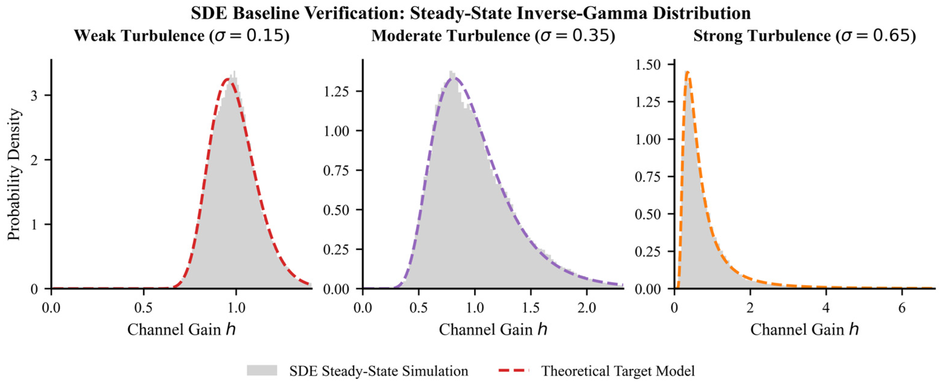
Simulations were conducted under the baseline multiplicative noise assumption ($\gamma =2.0$) across three distinct turbulence regimes: weak ($\sigma =0.15$), moderate ($\sigma =0.35$), and strong ($\sigma =0.65$). The time step was set to $\mathsf{\Delta }t=0.01$ over a duration of $T=2000$ units to ensure steady-state convergence.

As illustrated in Figure 3, the generated steady-state probability density functions (gray histograms) exhibit excellent agreement with the theoretical inverse-Gamma distributions (dashed curves) across all turbulence strengths. Notably, the simulation accurately captures the heavy-tailed characteristics inherent in strong turbulence regimes (Right panel of Figure 3). These results confirm two critical aspects:

(1)

Numerical Stability: The Euler–Maruyama solver maintains stability without divergence even under high-variance conditions.

(2)

Physical Consistency: The SDE correctly reproduces the classical statistical behavior of saturated turbulence when configured in the multiplicative noise regime.

This validates the proposed SDE solver as a reliable generative engine for the subsequent reinforcement learning training environment.

2.6. Numerical Fitting with Existing Models

To rigorously validate the effectiveness of the proposed SDE framework as a unified generative model for underwater optical turbulence, this study employed the Inverse Fokker–Planck equation method to conduct a systematic numerical validation. This method inversely reconstructs the drift dynamics term $\mu \left(h_t\right)$ required to reproduce the probability density functions (PDFs) of existing mainstream channel models. This approach demonstrates that the proposed SDE framework is capable of reproducing existing statistical models.

The capability of the proposed SDE to reproduce these diverse statistical distributions is not merely empirical. As derived analytically in Appendix B, the drift field $\mu \left(h\right)$ can be explicitly reconstructed from any target stationary PDF using the inverse Fokker–Planck equation, providing a mathematical basis for using the proposed SDE as a unified stochastic generator for a broad class of stationary channel statistics.

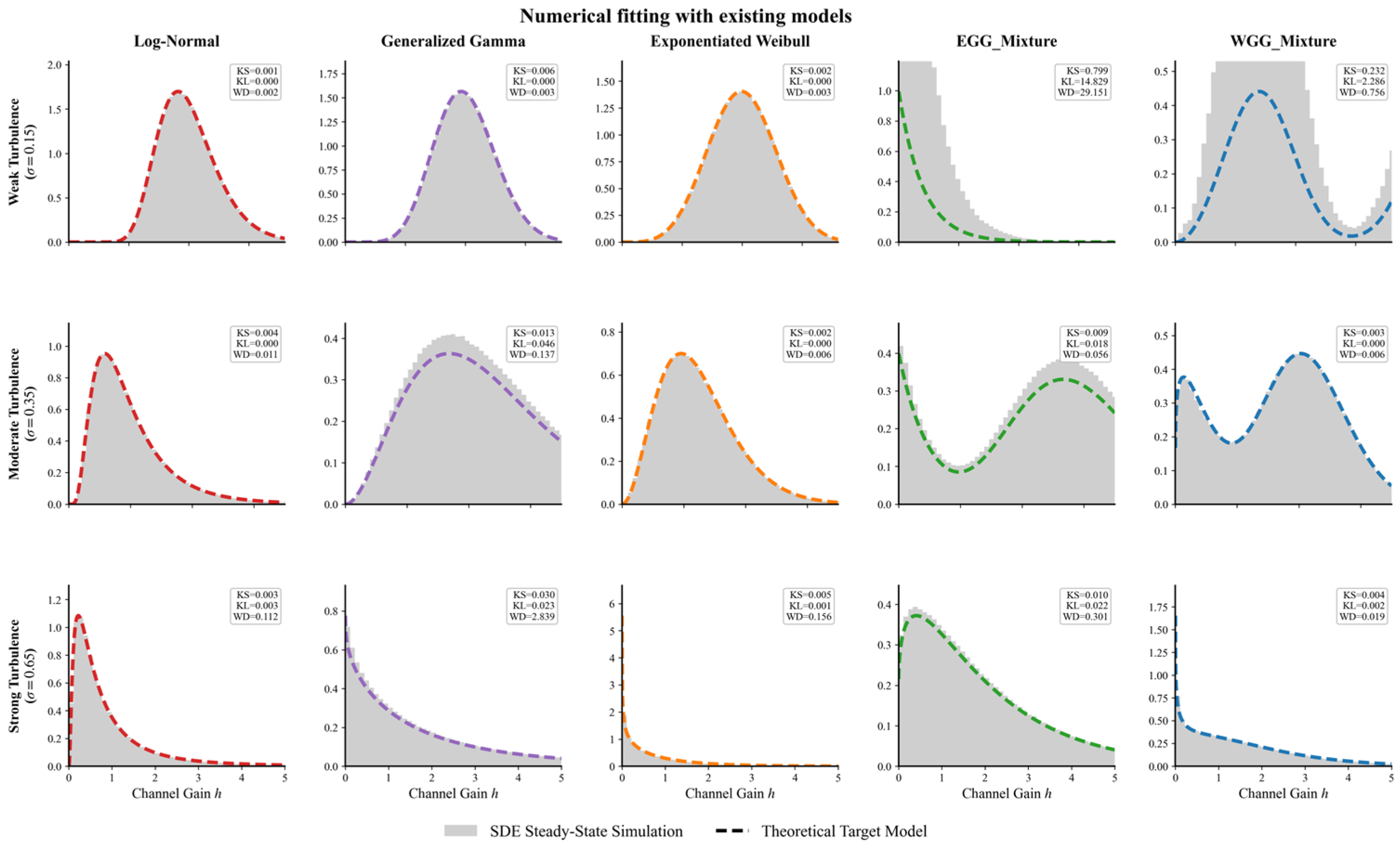
The validation process involved reconstructing the drift field $\mu \left(h\right)$ from five target theoretical distributions: log-normal (LN), generalized Gamma (GG), exponentiated Weibull (EW), and two mixture models—exponential generalized Gamma (EGG) and Weibull generalized Gamma (WGG). Three distinct turbulence regimes defined by the diffusion intensity coefficient $\sigma$ were simulated as follows. (1) Weak turbulence ($\sigma =0.15$): Simulating clear water with minimal refractive index fluctuations. (2) Moderate turbulence ($\sigma =0.35$): Representing typical coastal underwater environments. (3) Strong turbulence ($\sigma =0.65$): Representing scenarios with severe fading.

The simulation results, as illustrated in Figure 4, show that the proposed SDE framework can reproduce several target PDFs with good quantitative agreement in most tested cases. To avoid relying solely on visual histogram matching, the agreement was additionally quantified using the Kolmogorov–Smirnov (KS) statistic, Kullback–Leibler (KL) divergence, Jensen–Shannon (JS) divergence, and Wasserstein distance. For clarity, the KS, KL, and Wasserstein distance values are also displayed in the upper-right corner of each subplot in Figure 4. For the log-normal and exponentiated Weibull models, the fit remained consistently accurate across weak, moderate, and strong turbulence regimes, with KS values on the order of ${10}^{-3}$ and a very small KL divergence. The WGG and EGG mixture models were also reproduced well in most moderate-to-strong turbulence cases. However, noticeable deviations were observed for the weak-turbulence EGG mixture case and, to a lesser extent, the weak-turbulence WGG mixture case, indicating that the current multiplicative-noise SDE formulation is less effective for sharply separated or strongly skewed mixture structures in the near-deterministic regime.

For the log-normal model, the drift term exhibited an approximately linear balance between decay and compensation, which is consistent with the theoretical reduction in Section 2.3 and is supported by the very small KS and KL values obtained in all three turbulence regimes. For the EGG and WGG mixture models, the SDE retained the ability to reproduce bimodal or heavy-tailed structures in several moderate-to-strong turbulence cases. Nevertheless, the quantitative metrics reveal that this capability is not uniform across all regimes: in particular, the weak-turbulence EGG mixture case shows a large mismatch, and the weak-turbulence WGG mixture case also exhibits a non-negligible discrepancy. This suggests that, although nonlinear drift modulation captures many mixture-like behaviors without requiring a fully explicit jump-diffusion structure, additional model refinement may be needed for sharply separated mixture distributions under weak fluctuations.

The results also corroborate that the steady-state solution of the SDE belongs to the generalized Gamma family. By adjusting the drift-diffusion balance, the SDE can smoothly transition between the additive-noise-dominated Gamma limit ($\gamma \to 1$) and the multiplicative-noise-dominated inverse-Gamma limit ($\gamma \to 2$).

In conclusion, the quantitative results confirm that the proposed SDE can serve as a unified stochastic generator for several commonly used UWOC fading distributions, particularly log-normal, exponentiated Weibull, and a subset of generalized-gamma-based mixture models. The goodness-of-fit metrics demonstrate that the agreement is strong in most tested scenarios, while also revealing several failure cases in weak-turbulence mixture distributions and in heavy-tail matching under strong turbulence. We therefore emphasize that the distribution-matching capability of the model is broad but not universal in a strict sense. Its primary value lies in providing a single dynamic stochastic framework that reproduces a wide class of stationary channel statistics while retaining a physically interpretable baseline drift-diffusion structure.

3. Fuzzy-RL Hybrid Adaptive Controller

This section formulates the beam alignment task as a continuous-time stochastic control problem driven by SDEs. A hybrid Fuzzy-RL adaptive controller is proposed, and its key algorithmic procedures and theoretical properties are outlined.

3.1. Formulation of the Adaptive Optimization Problem

To address the complex time-varying turbulence and attitude disturbances in underwater optical communication systems, the present study treats the laser pointing control problem as an adaptive optimization process based on reinforcement learning. At the implementation level, the system adopts a decomposed structure with two independent subsystems for pitch and pan. A Fuzzy-RL controller is constructed for each axis. This design balances real-time performance, interpretability, and stability.

The two-dimensional motion of the laser pointing mechanism is jointly determined by the pitch angle ${\theta }_y$ and the yaw angle ${\theta }_x$. Theoretically, the complete state vector of the system should incorporate the coupled dynamics of both axes:

$$s\left(t\right)={\left[{\theta }_x,{\dot{\theta }}_x,{\theta }_y,{\dot{\theta }}_y,h\left(t\right)\right]}^T$$

(25)

where $h\left(t\right)$ represents the instantaneous power gain modeled by the SDE channel. The pitch and yaw channels of the gimbal driver exhibit near-decoupled characteristics. Dynamic coupling terms become significant only at high angular velocities or extreme attitudes. Furthermore, due to the excessive dimensionality of the full state vector, the subsequent reinforcement learning process would suffer from the curse of dimensionality in high-dimensional continuous space. To enhance sample training efficiency and ensure engineering feasibility, the present study adopts an axial decomposition strategy:

$$S=S_x\times S_y,A=A_x\times A_y$$

(26)

where each subsystem $\left(S_i,A_i\right)$ independently executes policy optimization. This enables parallel learning processes. This approximate factorization strategy is widely adopted in multivariate reinforcement learning and visual servo control. It ensures controller near-optimality while reducing computational burden and training time, demonstrating engineering feasibility.

For each axis, the state, action, and reward are defined as follows:

(1)

State variables define the state as $s_i\left(t\right)={\left[e_i\left(t\right),{\dot{e}}_i\left(t\right)\right]}^T$. Here, $e_i\left(t\right)$ represents the angular error of the laser spot relative to the target center, and ${\dot{e}}_i\left(t\right)$ denotes its time derivative. The state undergoes fuzzy partitioning before being input to the Fuzzy-RL controller. This reflects fuzzy membership degrees across different error levels.

(2)

Action variable (action): Let $a_i\left(t\right)$. This represents the angular fine-tuning increment for the current step. It is adjusted by the reinforcement learning module based on fuzzy outputs to achieve a dynamic balance between rapid response and steady-state performance.

(3)

State transition: The system dynamics are jointly determined by the closed-loop response of the gimbal servo mechanism and channel disturbances: $e_i\left(t+\mathsf{\Delta }t\right)=f_i\left(e_i\left(t\right),a_i\left(t\right),\xi \left(t\right)\right)$ where $\xi \left(t\right)$ denotes random disturbances caused by turbulence and observation noise.

Each subsystem optimizes to minimize the long-term cumulative error and control cost through the reinforcement learning process. The expected discounted return for a single axis is defined as

$$J_i=E\left[{{\displaystyle \sum }}_{t=0}^{\infty }{\mathsf{\beta }}^t{r}_i\left(s_i\left(t\right),a_i\left(t\right)\right)\right]$$

where the discount factor $\mathsf{\beta }\in \left(0,1\right)$ determines the planning horizon. Note: the symbol $\mathsf{\beta }$ is used here to distinguish it from the turbulence parameter $\mathsf{\gamma }$ defined in Section 2. The instantaneous reward function $r_i\left(\cdot \right)$ is designed to guide the agent:

$$r_i\left(t\right)=1-{\mathsf{\lambda }}_1{e}_i^2\left(t\right)-{\mathsf{\lambda }}_2\left|\dot{e_i}\left(t\right)\right|-{\mathsf{\lambda }}_3\left|a_i\left(t\right)\right|$$

The parameters ${\mathsf{\lambda }}_1$, ${\mathsf{\lambda }}_2$, and ${\mathsf{\lambda }}_3$ adjust the trade-off between accuracy, response speed, and energy consumption. Under the long-term statistical significance of channel gain $h\left(t\right)$, the expected total reward is the weighted sum of two independent subsystems:

$$J=w_x{J}_x+w_y{J}_y$$

(27)

where the weights $w_x$ and $w_y$ are determined by the sensitivity of system performance to optical axis geometry.

To achieve online adaptive control, the Fuzzy Logic Controller (FLC) provides empirical rules and nonlinear mapping capabilities. Meanwhile, the reinforcement learning module handles long-term strategy refinement.

For the single-axis subsystem $i$, the Fuzzy-RL integrated strategy can be expressed as

$$a_i\left(t\right)=F_i\left(e_i\left(t\right),{\dot{e}}_i\left(t\right)\right)+\mathsf{\Delta }{a}_{iRL}\left(t\right)$$

(28)

Here, $F_i\left(\cdot \right)$ is the fuzzy controller output, and $\mathsf{\Delta }{a}_{iRL}$ is the policy-based fine-tuning term from Q-learning. The Q-table value function is defined as

$$Q_i\left(s_i,a_i\right)=E\left[r_i\left(t\right)+\beta \underset{a_{i^{\prime }}}{\max }{Q}_i\left(s_{i^{\prime }},a_{i^{\prime }}\right)\right]$$

(29)

During learning, the Q-table is updated iteratively via temporal difference (TD) learning:

$$Q_i\left(s_i,a_i\right)\leftarrow Q_i\left(s_i,a_i\right)+\alpha \left[r_i\left(t\right)+\beta \underset{a_{i^{\prime }}}{\max }{Q}_i\left(s_{i^{\prime }},a_{i^{\prime }}\right)-Q_i\left(s_i,a_i\right)\right]$$

(30)

where $\alpha$ is the learning rate.

This decomposition structure mathematically corresponds to a factorized approximation of the global Q-function:

$$Q\left(s_x,s_y,a_x,a_y\right)\approx Q_x\left(s_x,a_x\right)+Q_y\left(s_y,a_y\right)$$

(31)

Such structures have been proven in distributed control and factored MDP research to yield near-optimal solutions under conditions of small coupling terms. Furthermore, the smoothness of the fuzzy layer ensures the policy is continuously differentiable in the input space. This satisfies local Lipschitz conditions, thereby guaranteeing the asymptotic bounded stability of the closed-loop system.

3.2. Fuzzy-RL Controller Design

The present study employs a hierarchical control architecture for each axis $i$. The lower layer consists of an interpretable Takagi–Sugeno (TS) fuzzy baseline $F_i$, while the upper layer utilizes a Q-learning-based fine-tuner $\mathsf{\Delta }{a}_i$. This design aims to combine interpretable empirical rules with data-driven adaptation while ensuring engineering feasibility. Consequently, it achieves steady-state accuracy and online adaptability under non-stationary channels and attitude disturbances.

Key Implementation:

(1)

TS Rule Form: The $j$ fuzzy rule is expressed as follows. Rule $j$: If $e_i$ is $A_j$ AND ${\dot{e}}_i$ is $B_j$, then $y_j=W_{jT}{\phi }_i+b_j$, where ${\phi }_i={\left[e_i,{\dot{e}}_i\right]}^T$. The final baseline output is the weighted sum of linear consequents.

(2)

Membership Functions: Gaussian membership functions are employed. Their centers are determined by offline clustering, and widths are set according to coverage and overlap criteria.

(3)

Fuzzy Parameter Strategy: By default, the membership structures are frozen, and only the consequent parameters are fine-tuned to ensure reproducibility. As an optional control experiment, the consequent parameters may undergo online projection updates with a small learning rate.

3.3. Reinforcement Learning Component Design

This section focuses on the minimalist yet sufficient design of the RL module for each axis. Key aspects include state and action definitions, reward structures, learning laws, and exploration strategies. The objective is to ensure sample efficiency and online stability.

State: The state vector $s_i={\left[\mathrm{Index}\left(e_i\right),\mathrm{Index}\left(\dot{e_i}\right)\right]}^T$ employs fuzzy indexing to discretize continuous error dynamics, balancing interpretability with computational efficiency. The channel state $h\left(t\right)$ is excluded from this RL state space to mitigate the curse of dimensionality, as it is independently managed by the supervisor module.

Actions: The action space consists of a discrete step set. Symmetric subdivided step sizes are used in the experiments.

Reward Design: The immediate reward takes a physically and task-driven weighted form:

$$r_i=clip\left(1-{\lambda }_p{e}_{i2}-{\lambda }_d\mid {\dot{e}}_i\mid -{\lambda }_a\mid a_i\mid ,r_{\min },r_{\max }\right)$$

(32)

This function penalizes large errors, rapid changes, and excessive control efforts.

Primary Approach: Tabular Q-learning is selected as the most robust choice for low-dimensional states. The temporal difference (TD) update is given by

$$Q\left(s,a\right)\leftarrow Q\left(s,a\right)+\alpha \left(r+\gamma \underset{a^{\prime }}{\max }Q\left(s^{\prime },a^{\prime }\right)-Q\left(s,a\right)\right)$$

(33)

Exploration: Boltzmann softmax with temperature annealing is employed. An $ϵ$-greedy strategy serves as a control baseline. In the present implementation, Boltzmann softmax with temperature annealing is adopted as the exploration strategy, while an $\epsilon$-greedy policy is used as a baseline for comparison. The controller is trained offline prior to HIL deployment using repeated stochastic channel realizations generated by the SDE environment. The tabular Q-learning policy uses a fixed discrete action set and bounded rewards, while the exploration temperature is annealed during training and then frozen during evaluation. The PID baseline is tuned separately under the same plant and disturbance model to provide a fair closed-loop comparison.

At the implementation level, the deployed HIL prototype used a tabular Q-learning controller with Gaussian fuzzy partitioning and a fixed discrete action set for each axis. In the present prototype, 11 fuzzy labels were used for the error and error-rate variables, together with a seven-level discrete action set. The learning rate and discount factor were set to 0.005 and 0.95, respectively, and Boltzmann temperature annealing was employed during training. To improve robustness under camera delay and embedded execution constraints, several engineering stabilizers were additionally introduced in the real system, including latency-compensated state extrapolation, command smoothing, damping, dead-zone logic, and a fallback proportional-integral action outside the safe exploration region. These settings should be interpreted as practical deployment choices for the HIL prototype rather than as part of the abstract theoretical formulation.

Under conditions of finite states, bounded rewards, and appropriate learning rate decay, tabular Q-learning converges to a suboptimal neighborhood of the Bellman fixed point for each axis. This deviation is primarily due to fuzzy approximation errors.

3.4. Compact Pseudocode

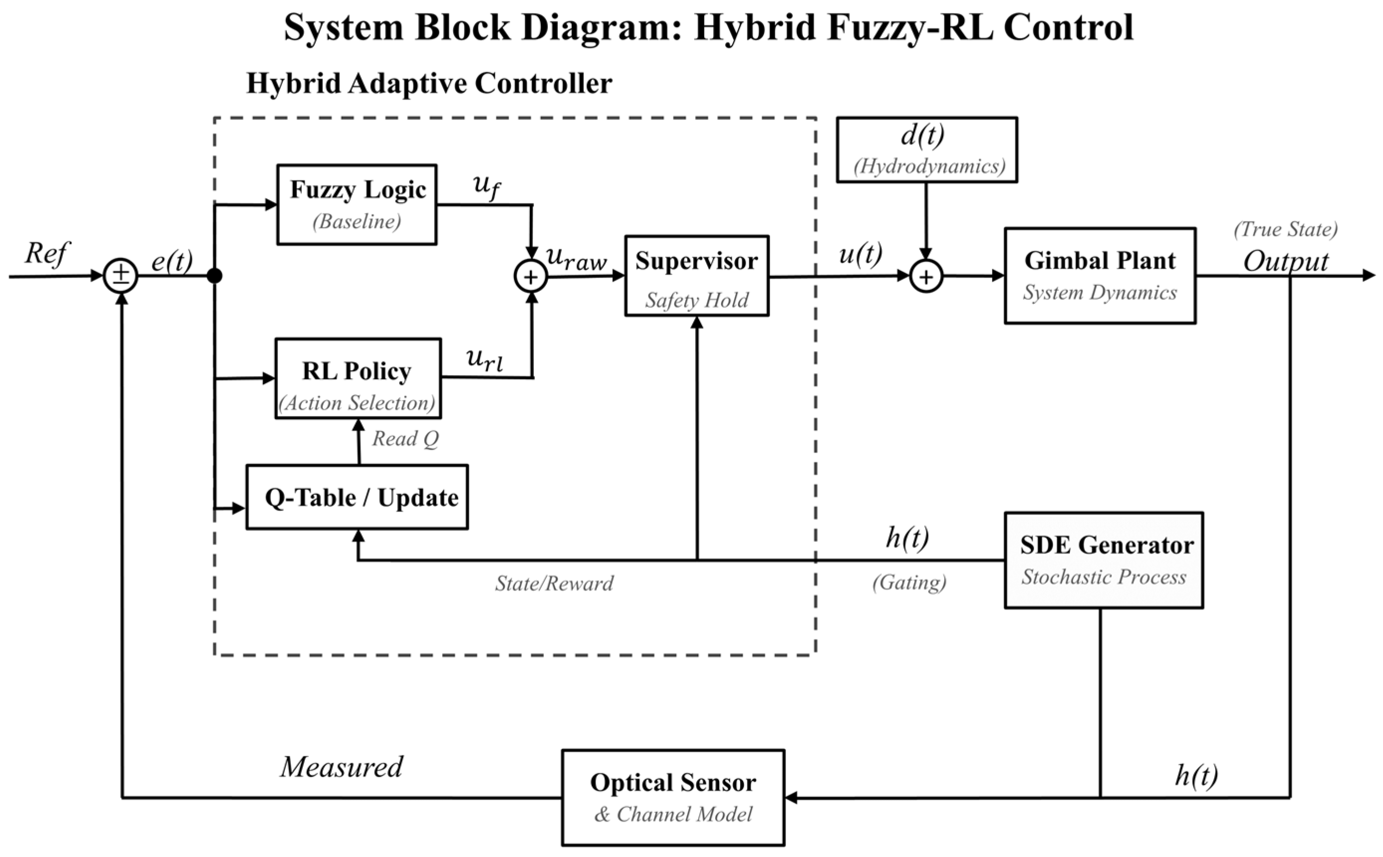
To intuitively visualize the implementation logic, the control block diagram of the proposed hybrid adaptive controller is presented in Figure 5. This diagram illustrates the signal flow integrating the fuzzy baseline, RL fine-tuning, and the safety-hold mechanism.

To explicitly handle non-stationary disturbances, we adopt a hierarchical supervision strategy that decouples kinematic optimization from safety assurance.

Optimization Layer (Fuzzy-RL): Active when the channel is reliable, the RL agent fine-tunes control actions based on error dynamics to minimize tracking deviation.

Safety layer (supervisor): Monitors channel gain $h\left(t\right)$ and overrides RL output with a “Safety-Hold” policy during deep fading. This separation prevents the agent from learning noise-induced policies during signal loss, eliminating the need to explore rare failure modes.

3.5. Computational Complexity Analysis

The proposed Fuzzy-RL controller executes three sequential modules at each control step: fuzzy inference, Q-table-based reinforcement learning, and supervisor override logic. Their computational complexities are analyzed below.

For the fuzzy inference engine, let $n$ denote the number of input variables, $m$ the number of membership functions per input, and $r$ the number of active fuzzy rules. The fuzzification stage requires $O\left(nm\right)$ operations, while rule activation, aggregation, and centroid defuzzification require $O\left(r\right)$ operations. Therefore, the per-step complexity of the fuzzy module is

$$T_{\mathrm{fuzzy}}=O\left(nm+r\right)$$

(34)

In the present implementation, $n=2$, $m=5$, and $r=25$, so the fuzzy inference cost is effectively constant per control cycle.

For the RL module, the controller maintains a Q-table of size $\left|S\right|\times \left|A\right|$, where $\left|S\right|$ and $\left|A\right|$ denote the numbers of discrete states and actions, respectively. Action selection under an $\epsilon$-greedy policy requires $O\left(\left|A\right|\right)$ comparisons, whereas the temporal-difference update requires $O\left(1\right)$ time. Thus,

$$T_{\mathrm{RL}}=O\left(\left|A\right|\right)$$

(35)

With $\left|S\right|=400$ and $\left|A\right|=5$ in our implementation, the total storage required for the Q-table is approximately 16 KB in double precision, which is negligible for embedded hardware.

The supervisor logic only involves a threshold comparison on $h\left(t\right)$ and a timer check, both of which are constant-time operations, i.e., $O\left(1\right)$.

Accordingly, the overall computational complexity per control step is

$$T_{\mathrm{total}}=O\left(nm+r+\left|A\right|\right)$$

(36)

For fixed hyperparameters, this simplifies to $O\left(1\right)$, indicating constant-time execution during online control.

Compared with MPC, whose per-step computational burden typically scales as $O\left(N_p{n}_x^3\right)$ due to repeated online optimization, and with deep RL methods, whose inference cost scales with network depth and width as $O\left({\displaystyle {\displaystyle \sum }_l}{d}_{l-1}{d}_l\right)$, the proposed method is substantially more lightweight. Therefore, the proposed Fuzzy-RL controller combines adaptive capability with low online computational cost, making it suitable for real-time deployment on resource-limited AUV embedded processors.

3.6. Theoretical Analysis and Innovations

Under Assumptions A1–A3 stated in Appendix A.1 and the reduced plant model adopted in this study, the proposed hybrid scheme guarantees mean-square boundedness of the closed-loop error and asymptotic convergence to a bounded neighborhood, as established via the Lyapunov analysis in Appendix A.

Compared with deep RL approaches that require function approximation and larger memory footprints, the present tabular Fuzzy-RL design has a modest computational complexity that is compatible with real-time embedded implementation. A full runtime benchmark against deep RL variants is left for future work.

4. Results

4.1. Numerical Simulation and Controller Benchmarking

Before deploying the control algorithms on the hardware-in-the-loop (HIL) testbed, a comparative numerical simulation was conducted to benchmark the robustness of the proposed Fuzzy-RL framework against PID, anti-windup PID, ADRC, and MPC baselines. The simulation environment utilizes the discrete SDE channel generator verified in Section 2, ensuring that the disturbance dynamics reflect realistic underwater optical turbulence and fading characteristics.

While classical linear controllers perform adequately under continuous Gaussian turbulence, their performance often degrades catastrophically during discontinuous disturbances common in underwater environments, such as air bubble occlusion or sudden turbidity plumes.

To evaluate the system’s resilience to such non-stationary events, a “Deep Fading” test scenario was constructed:

(1)

Channel Dynamics: A baseline moderate turbulence $\sigma =0.35$ is generated. A forced “bubble blockage” event is introduced between $t=3.0$ s and $t=5.0$ s, during which the channel gain drops to near zero ($h\left(t\right)\approx 0.05$), simulating a complete signal interruption.

(2)

Sensor Noise: During the blockage, the vis feedback is assumed to be unreliable, outputting random measurement noise or drifting values.

(3)

Baselines: the pre-trained Fuzzy-RL controller was benchmarked against PID, anti-windup PID, ADRC, and MPC under the same plant and disturbance setup.

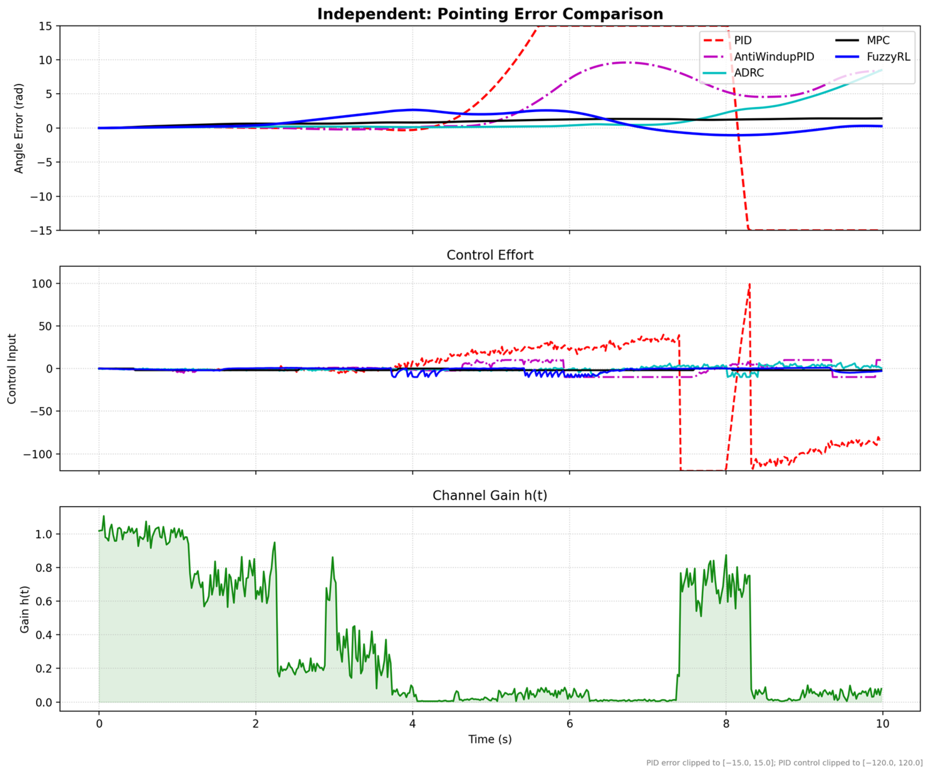
The simulation results, illustrated in Figure 6, provide a representative time-domain comparison of the five controllers under the SDE-driven deep-fading benchmark. A clear performance hierarchy can be observed during the signal-loss and recovery stages.

Among the classical baselines, the conventional PID controller exhibits the most severe degradation. Because it has no explicit supervision mechanism for channel reliability, it continues to integrate noisy error signals during the low-gain interval, leading to pronounced windup. As shown in the top and middle panels of Figure 6, this accumulated control effort is released abruptly after channel recovery, producing the largest overshoot and the most oscillatory actuator response.

The anti-windup PID controller alleviates this issue to some extent, reducing the peak excursion after recovery; however, its transient error remains noticeably larger than that of the more advanced controllers. ADRC and MPC both provide substantially improved recovery behavior, with smaller overshoot and smoother control effort than the two PID-based baselines. Nevertheless, both methods still show visible transient deviation during the fading-to-recovery transition.

By comparison, the proposed Fuzzy-RL controller delivers the most balanced closed-loop response. It maintains the smallest pointing-error excursion during recovery while avoiding the large control spikes observed in PID. This behavior is consistent with the intended role of the supervisor mechanism, which suppresses unreliable corrective action when the channel state becomes severely degraded and enables smoother target re-acquisition once the optical link is restored.

Therefore, Figure 6 visually confirms the broader benchmarking results reported in Section 4.2: incorporating channel-state awareness into the control policy is essential for maintaining tracking robustness under deep fading, and the proposed Fuzzy-RL framework provides the best overall trade-off between alignment accuracy, recovery smoothness, and control effort. These communication-level quantities should be interpreted as model-based indicators derived from the closed-loop channel state, rather than as direct measurements from a complete IM/DD receiver chain.

4.2. Controller Robustness and Parameter Sensitivity Analysis

To further evaluate the proposed hybrid Fuzzy-RL algorithm under the complexity of underwater environments, this section presents a series of multidimensional stress tests based on Monte Carlo simulations with $n=20$ trials. In addition to benchmarking against several classical and modern control algorithms, the study also comprehensively assesses the sensitivity of the proposed method to stochastic channel parameters, controller hyperparameters, and measurement noise.

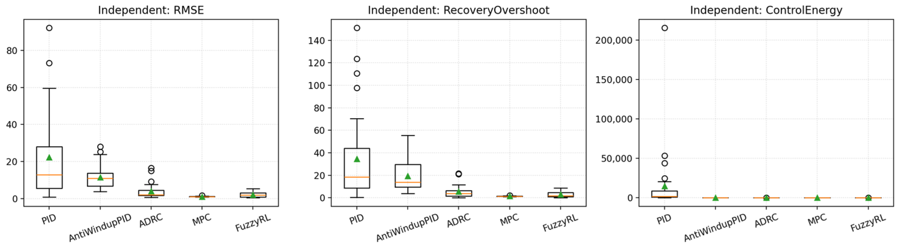
To evaluate the relative performance of the proposed method within the broader control framework, two representative scenarios were considered: a continuous fluctuation environment driven by the SDE channel model and an extreme deep-fading environment with Markov jump bursts. In these two scenarios, the proposed controller was compared with conventional PID, anti-windup PID, active disturbance rejection control (ADRC), and model predictive control (MPC). The corresponding simulation results are shown in Figure 7.

The results demonstrate that, in the nominal turbulence channel driven by the SDE model, the Fuzzy-RL controller achieves the best alignment accuracy. Its root-mean-square error (RMSE) is only 0.4256 mm, and its median absolute error is as low as 0.1449 mm. By contrast, the RMSE values of conventional PID and anti-windup PID are 4.5406 mm and 4.2847 mm, respectively, both accompanied by deep-fading recovery overshoots of approximately 10.12–14.03 mm. Compared with ADRC, which represents a robust-control baseline (RMSE = 1.3365 mm), and MPC, which represents an optimal-control baseline (RMSE = 0.8644 mm), the proposed Fuzzy-RL method reduces the RMSE by more than 50%. Although MPC exhibits a lower control energy consumption (control energy = 2.3760), Fuzzy-RL (control energy = 6.4873) achieves more accurate steady-state tracking while maintaining reasonable computational overhead and completely avoiding alignment failure.

Under the extreme burst-disturbance scenario, which includes Markov jumps and severe communication outages, the conventional controllers exhibit widespread failure, with failure rates exceeding 95%. In contrast, the proposed Fuzzy-RL controller still maintains a median absolute error of 0.8710 mm. This result confirms that the supervisor mechanism can effectively suppress divergence under severe data-loss conditions.

To investigate whether the background assumptions of the model may lead to performance degradation under different ocean conditions, a wide parameter scan was conducted over the key drift and diffusion coefficients of the SDE channel model. This analysis was used to evaluate the sensitivity of the controller to stochastic channel parameters.

For the drift and mean-reversion coefficients $\left(a,b\right)$, when the mean-reversion rate varies within e and the intensity scale varies within $b\in \left[0.7,1.3\right]$, the performance metrics remain highly flat. In this range, the RMSE is tightly confined to 0.4224–0.4247 mm, and the recovery overshoot varies by less than 0.02 mm.

For the turbulence diffusion and fluctuation-intensity parameters $\left(k,\gamma \right)$, with $k\in \left[0.18,0.5\right]$ and $\gamma \in \left[0.7,1.3\right]$, the corresponding joint heat map shows that the closed-loop RMSE remains stable within 0.4227–0.4248 mm. These results indicate that the unified stochastic generator reconstructed through the inverse Fokker–Planck method has strong generalization capability and that the controller does not rely on any specific form of turbulence probability density function (PDF).

In practical engineering deployment, sensor noise often constitutes a major source of instability. The experimental results show that the proposed control architecture has a high degree of tolerance to observation noise. When the measured channel-state fading-noise envelope, denoted as loss minus noise e, increases from 0.25 to 0.75, the statistical RMSE remains at approximately 0.4235 mm. This indicates that the fuzzy logic layer effectively filters high-frequency clutter before it propagates into the RL action space.

The proposed controller also exhibits strong robustness to variations in internal control gains. Specifically, when the proportional gain of the lower-level controller varies within $K_p\in \left[6.0,9.5\right]$, the damping coefficient of the deep-fading supervisor varies within $holddamping\in \left[0.2,1.0\right]$, and the recovery gain varies within $boostgain\in \left[1.0,1.7\right]$, the resulting performance degradation remains minimal, with an RMSE variation range of less than 0.02 mm. This result demonstrates strong environmental adaptability and suggests that the controller does not require stringent online retuning in different operating conditions.

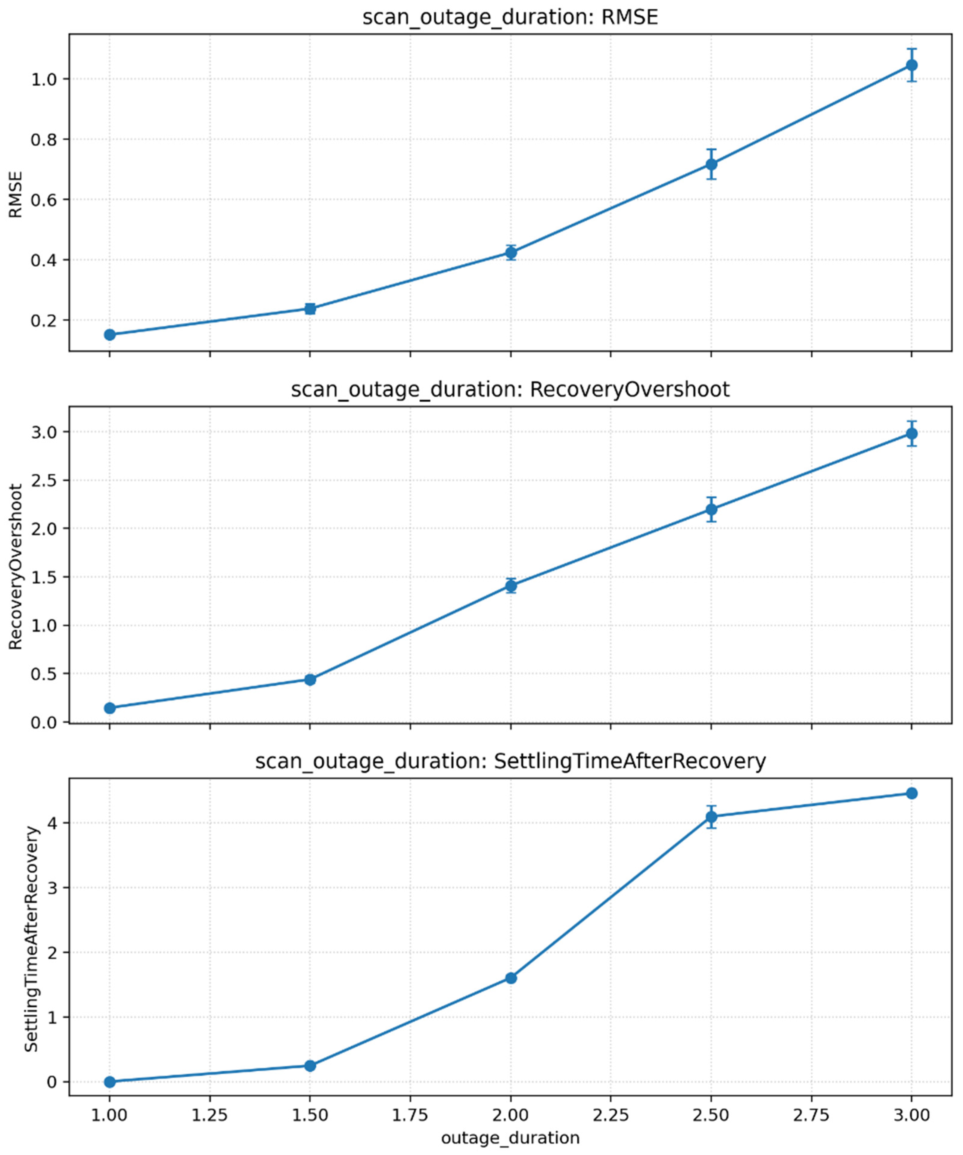
When the forced deep-fading duration, denoted as outage duration, increases from 1.0 s to 3.0 s, random platform jitter gradually becomes dominant because the optical feedback is unavailable for an extended period. As a result, the RMSE increases from 0.1510 mm to 1.0459 mm, while the recovery overshoot rises from 0.1469 mm to 2.9819 mm. This result objectively reflects the physical limitation of purely optical feedback under prolonged deep-fading conditions. It also suggests that, once the outage duration exceeds a threshold of approximately 2–3 s, additional inertial measurement units or other sensing modalities should be introduced to enable multi-source hardware fusion and maintain closed-loop stability. The corresponding sensitivity results for RMSE, recovery overshoot, and settling time are shown in Figure 8.

4.3. Hardware-in-the-Loop (HIL) Experimental Setup

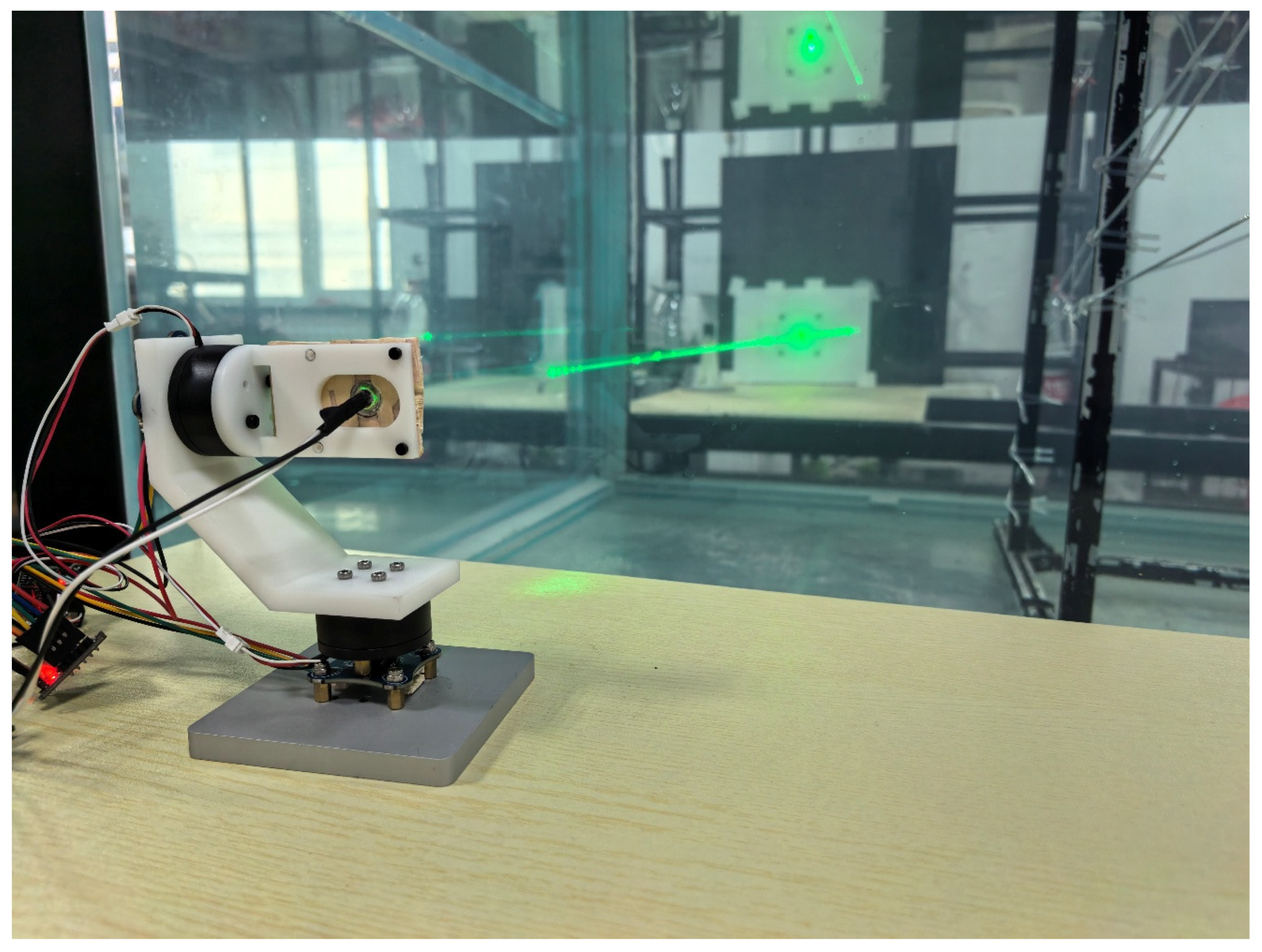
To validate the practical performance of the proposed unified SDE channel model and hybrid Fuzzy-RL controller, a two-degree-of-freedom (2-DOF) laser-pointing hardware-in-the-loop (HIL) platform was constructed. The platform consists of the following main components. The prototype system and experimental environment are shown in Figure 9.

A 2-DOF gimbal was built using an ESP32 microcontroller (Espressif Systems, Shanghai, China), 2804-type brushless DC (BLDC) motors with seven pole pairs, and AS5600 magnetic encoders. The motors were controlled using the SimpleFOC library to realize closed-loop angle control and field-oriented current control under a 12 V supply. The embedded controller transmitted real-time encoder angles to the host computer using Python 3.11.14 via serial communication every 5 ms, ensuring an accurate low-level control cycle.

An industrial camera with a resolution of 640 × 480 was employed for visual feedback. The measured frame rate was approximately 30 fps, with an average frame-capture delay of about 92 ms (approximated as 100 ms in the control code). The corresponding horizontal and vertical fields of view were 60° and 45°, respectively. The camera was placed at a fixed distance of 0.18 m from the target plane for ArUco marker detection and laser-spot localization.

A green Osram PLT5 laser diode operating at 520 nm with an output power of 80 mW was used as the transmitter. The laser source was powered by a constant-current driver module. The distance from the laser emitter to the target plane was fixed at 2.0 m.

The experiments were conducted in a clear-water tank with a length of approximately 2 m. According to the optical properties of the green wavelength band and representative literature values, the water attenuation coefficient (absorption + scattering) was set to approximately $c\approx 0.08 {\mathrm{m}}^{-1}$. For a 2 m propagation distance, this corresponds to a total power attenuation of about 15% $\left(e^{-cL}\approx 0.85\right)$, representing a weak-to-moderate turbulence multiple-scattering condition.

ArUco markers from the 4 × 4 dictionary were used for spatial calibration. A multi-frame averaging strategy based on more than 20 frames was adopted to estimate the physical spacing between the four marker centers (110 mm), thereby obtaining the pixel-to-millimeter conversion factor automatically. Laser-spot detection was implemented using HSV color thresholding, morphological processing, and weighted centroid estimation, combined with dynamic region-of-interest (ROI) tracking. The pointing error was then converted from pixel deviation into physical angular and positional deviation.

Throughout the experiments, the host computer recorded the control commands, encoder feedback, pixel-domain and physical-domain tracking errors, frame delay, SDE-generated channel gain $h\left(t\right)$, Fuzzy-RL reward values, and exploration temperature parameters, ensuring full reproducibility of the reported results. In the HIL framework, the SDE model generated $h\left(t\right)$ online and injected it into the feedback loop in real time. Therefore, the present setup should be interpreted as a model-in-the-loop validation of the closed-loop architecture rather than a purely physical channel emulation. This choice is intentional: the HIL platform is used to evaluate controller robustness under controlled and repeatable stochastic excitation before open-water deployment, rather than to claim independent validation of the channel model itself. In other words, the SDE-driven channel serves as a calibrated digital test environment for closed-loop benchmarking, while independent long-range ocean measurements remain necessary for future external validation of the channel physics. The main hardware and experimental parameters of the HIL platform are summarized in

Table 2. Summary of main experimental parameters.

Parameter	Value/Specification	Remarks
Gimbal actuator	2804 BLDC + AS5600	SimpleFOC closed-loop control, feedback every 5 ms
Camera	640 × 480 @ 30 fps	Measured frame delay ≈ 92 ms, FOV 60°/45°
Camera–target distance	0.18 m	Used for ArUco and spot detection
Laser–target distance	2.0 m	Tank-scale propagation path
Laser source	520 nm, 80 mW	Constant-current driven
Water type	Clear water	Attenuation coefficient $c\approx 0.08 {\mathrm{m}}^{-1}$
ArUco physical spacing	110 mm	Used for pixel-scale calibration
Control cycle	5 ms (embedded)/~33 ms (camera)	Fusion of serial and visual feedback

.

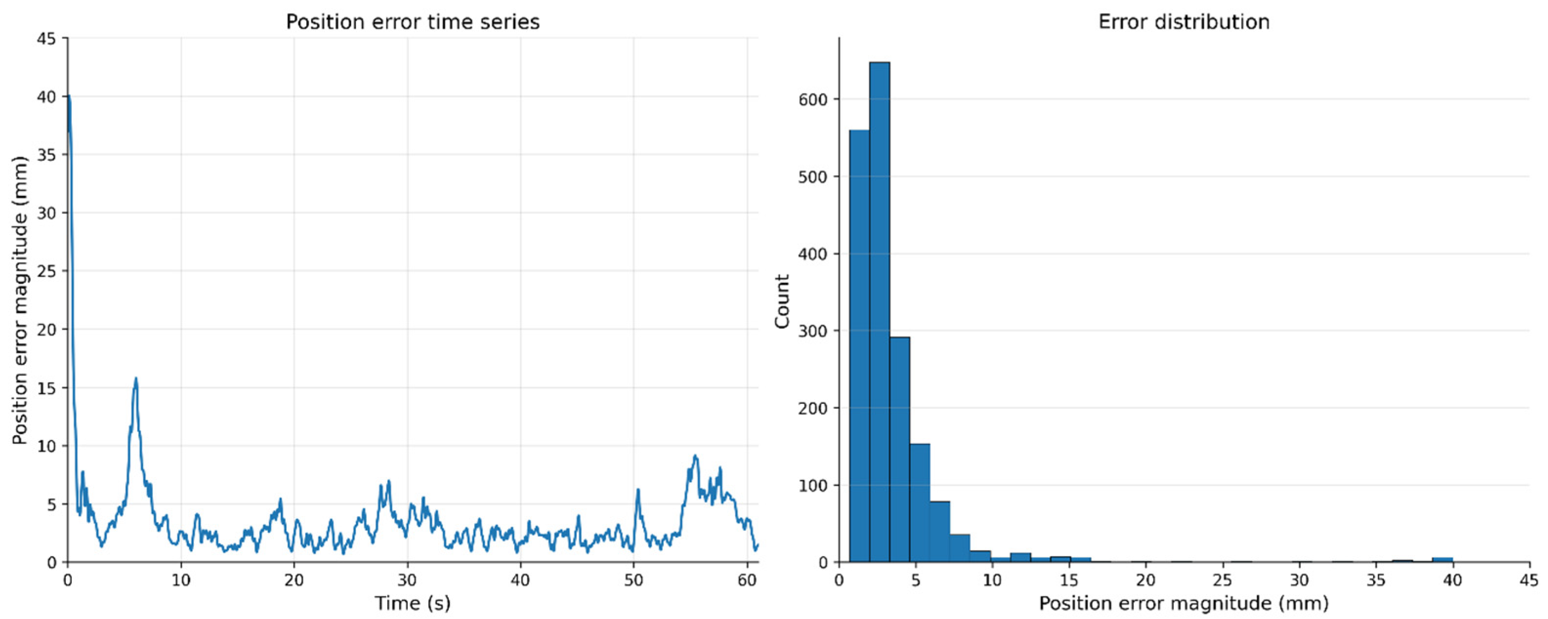
The system achieved an average alignment error of $e\approx 5.26\mathrm{mm}$, with a standard deviation of ${\mathsf{\sigma }}_{\mathrm{e}}\approx 6.18\mathrm{mm}$ and a median of $\mathrm{median}\left(e\right)\approx 3.64\mathrm{mm}$. During the initialization phase, an initial offset was set at startup $e_{max}\approx 40\mathrm{mm}$, and the system rapidly compensated for it. However, a time delay from image acquisition to error data retrieval was observed due to limitations of the computing platform and data transmission protocol. This delay was identified as a cause of steady-state oscillations. Future improvements could involve adopting higher-speed transmission protocols to enhance control performance or employing methods like Kalman filtering to predict and compensate for time delays. A median error of approximately 3.6 mm indicates that the visual outer loop maintains alignment within a narrow range for the vast majority of the time. However, the mean value was slightly elevated by a few sporadic events. This suggests a potential need for more robust detection and filtering in subsequent iterations. The summary statistics of the closed-loop pointing error are listed in

Table 3. Summary statistics of the HIL closed-loop pointing error.

Metric	Value
Average alignment error	$e\approx 5.26\mathrm{mm}$
Standard deviation	${\sigma }_{\mathrm{e}}\approx 6.18\mathrm{mm}$
Median	$\mathrm{median}\left(e\right)\approx 3.64\mathrm{mm}$

. The temporal evolution and statistical distribution of the HIL pointing error are further illustrated in Figure 10, including the time-series response and the corresponding error histogram.

5. Conclusions

In this paper, a unified stochastic dynamic framework and a hybrid intelligent control strategy are proposed to address the challenges of underwater wireless optical communication (UWOC) in turbulent environments. By bridging the gap between the physical Radiative Transfer Equation (RTE) and control-oriented state-space models, a physically motivated stochastic differential equation (SDE) representation of the optical channel was derived.

The study yields three primary contributions. First, the derived SDE is demonstrated to serve as a “unified stochastic generator” for optical turbulence. Through the inverse Fokker–Planck equation approach, the model successfully reconstructs drift fields for a broad class of target statistical distributions—including log-normal, Gamma–Gamma, and mixture models—thereby capturing the temporal evolution of channel fading that static models fail to describe. Second, the beam alignment task is reformulated as the stabilization of a stochastic nonlinear system under multiplicative noise. The proposed hybrid Fuzzy-Reinforcement Learning (Fuzzy-RL) strategy effectively integrates the interpretability of fuzzy logic with the adaptive optimization of Q-learning. Finally, hardware-in-the-loop (HIL) experiments confirmed the practical viability of the framework, achieving pointing accuracy with a median alignment error of 3.64 mm.

The implications of this work extend beyond specific experimental results. Theoretically, the transition from static probability density functions to dynamic SDEs represents a paradigm shift in modeling random media. While traditional models quantify how often fading occurs, the unified SDE framework elucidates how the channel evolves, providing the essential derivative information required for predictive control. Practically, compared to end-to-end DRL methods that demand substantial GPU resources, the hybrid architecture remains computationally lightweight, making it highly suitable for the resource-constrained embedded systems typical of AUVs.

Despite these advances, some limitations remain. The current experimental setup observed minor steady-state oscillations. Future iterations could incorporate predictive filters, such as Kalman filtering, to compensate for sensor latency. Additionally, while this study focused on a single point-to-point link, the SDE framework is naturally extensible. Future research will explore the application of deep Fuzzy-RL architectures to multi-AUV coordination, investigating how distributed stochastic control can maintain mesh network connectivity in complex, scattering-dominant ocean environments. Several limitations should be noted. First, the diffusion-approximation-based channel reduction is most appropriate in multiple-scattering regimes and may lose accuracy in highly anisotropic or bubble-dominant waters. Second, the present HIL platform validates the controller under controlled laboratory conditions rather than in open-water long-range deployment. Third, BER and capacity are inferred from simplified communication-level proxies and were not directly measured with a complete IM/DD receiver chain. Finally, the reduced AUV–gimbal coupling model and Gaussian baseline diffusion term provide an engineering abstraction, not a full description of all intermittent ocean-turbulence mechanisms.

In summary, this work provides a physically motivated and control-oriented stochastic framework for UWOC beam-pointing analysis and control, and it offers a practical basis for future open-water validation and multi-sensor extensions.

References

1. Ishimaru, A. Wave Propagation and Scattering in Random Media; Academic Press: Cambridge, MA, USA, 1978. [Google Scholar]
2. Garnier, J. Wave propagation in random media: Beyond Gaussian statistics. ESAIM Proc. Surv. 2023, 74, 63–89. [Google Scholar] [CrossRef]
3. Wynn, R.B.; Huvenne, V.A.I.; Le Bas, T.P.; Murton, B.J.; Connelly, D.P.; Bett, B.J.; Ruhl, H.A.; Morris, K.J.; Peakall, J.; Parsons, D.R.; et al. Autonomous Underwater Vehicles (AUVs): Their past, present and future contributions to the advancement of marine geoscience. Mar. Geol. 2014, 352, 451–468. [Google Scholar] [CrossRef]
4. Yan, T.; Xu, Z.; Yang, S.X.; Gadsden, S.A. Formation control of multiple autonomous underwater vehicles: A review. Intell. Robot. 2023, 3, 1–22. [Google Scholar] [CrossRef]
5. Jamali, M.V.; Mirani, A.; Parsay, A.; Abolhassani, B.; Nabavi, P.; Chizari, A.; Khorramshahi, P.; Abdollahramezani, S.; Salehi, J.A. Statistical studies of fading in underwater wireless optical channels in the presence of air bubble, temperature, and salinity random variations. IEEE Trans. Commun. 2018, 66, 4706–4723. [Google Scholar] [CrossRef]
6. Qiu, H.; Huang, Z.; Xu, J.; Zhai, W.; Gao, Y.; Ji, Y. Unified statistical thermocline channel model for underwater wireless optical communication. Opt. Lett. 2023, 48, 636–639. [Google Scholar] [CrossRef]
7. Boluda-Ruiz, R.; García-Zambrana, A.; Castillo-Vázquez, B.; Hranilovic, S. Impact of angular pointing error on BER performance of underwater optical wireless links. Opt. Express 2020, 28, 34606–34622. [Google Scholar] [CrossRef] [PubMed]
8. Ijeh, I.C.; Khalighi, M.A.; Elamassie, M.; Hranilovic, S.; Uysal, M. Outage probability analysis of a vertical underwater wireless optical link subject to oceanic turbulence and pointing errors. J. Opt. Commun. Netw. 2022, 14, 439–453. [Google Scholar] [CrossRef]
9. Al-Habash, M.A.; Andrews, L.C.; Phillips, R.L. Mathematical model for the irradiance probability density function of a laser beam propagating through turbulent media. Opt. Eng. 2001, 40, 1554–1562. [Google Scholar] [CrossRef]
10. Zedini, E.; Oubei, H.M.; Kammoun, A.; Hamdi, M.; Ooi, B.S.; Alouini, M.S. Unified statistical channel model for turbulence-induced fading in underwater wireless optical communication systems. IEEE Trans. Commun. 2019, 67, 2893–2907. [Google Scholar] [CrossRef]
11. Arya, V. A comprehensive review on underwater optical wireless communication (UOWC) systems: Present and future prospective. J. Opt. Commun. 2025. [Google Scholar] [CrossRef]
12. Lou, Y.; Cheng, J.; Nie, D.; Qiao, G. Performance of underwater wireless optical communications in presents of cascaded mixture exponential-generalized gamma turbulence. arXiv 2020, arXiv:2008.02868. [Google Scholar] [CrossRef]
13. Alheadary, W.G.; Park, K.H.; Alouini, M.S. Performance analysis of multihop heterodyne free-space optical communication over general Malaga turbulence channels with pointing error. Optik 2017, 151, 34–47. [Google Scholar] [CrossRef]
14. Le-Tran, M.; Kim, S. Performance analysis of multi-hop underwater wireless optical communication systems over exponential-generalized gamma turbulence channels. IEEE Trans. Veh. Technol. 2022, 71, 6214–6227. [Google Scholar] [CrossRef]
15. Cochenour, B.; Mullen, L.; Muth, J. Temporal response of the underwater optical channel for high-bandwidth wireless laser communications. IEEE J. Ocean. Eng. 2013, 38, 730–742. [Google Scholar] [CrossRef]
16. Vali, Z.; Michelson, D.; Ghassemlooy, Z.; Noori, H. A survey of turbulence in underwater optical wireless communications. Optik 2025, 320, 172126. [Google Scholar] [CrossRef]
17. Meyers, B.; Mangelson, J.G. Testing and Evaluation of Underwater Vehicle Using Hardware-in-the-Loop Simulation with HoloOcean. arXiv 2025, arXiv:2511.07687. [Google Scholar]
18. Orjales, F.; Rodríguez-Cortegoso, J.; Fernández-Pérez, E.; Romero, A.; Diaz-Casas, V. Towards a Digital Twin for Open-Frame Underwater Vehicles Using Evolutionary Algorithms. Appl. Sci. 2025, 15, 7085. [Google Scholar] [CrossRef]
19. Almonacid, L.; Játiva, P.P.; Azurdia-Meza, C.A.; Dujovne, D.; Soto, I.; Firoozabadi, A.D.; Gaitan, M.G. On the path loss performance of underwater visible light communication schemes evaluated in several water environments. In 2023 South American Conference On Visible Light Communications (SACVLC); IEEE: Piscataway, NJ, USA, 2023; pp. 12–16. [Google Scholar]
20. Martínez, G.; Játiva, P.P.; Gaitán, M.G.; Meza, C.A.; Boettcher, N.; Zabala-Blanco, D. On the Performance of an Air-Water Visible Light Communication System. In Advanced Research in Technologies, Information, Innovation and Sustainability; Springer Nature: Cham, Switzerland, 2024; pp. 380–394. [Google Scholar]
21. Dimitropoulos, D.; Jalali, B. Stochastic differential equation approach for waves in a random medium. Phys. Rev. E Stat. Nonlinear Soft Matter Phys. 2009, 79, 036606. [Google Scholar] [CrossRef]
22. Borcea, L.; Garnier, J. Derivation of a one-way radiative transfer equation in random media. Phys. Rev. E 2016, 93, 022115. [Google Scholar] [CrossRef]
23. Enghiyad, N.; Sabbagh, A.G. Impulse response of underwater optical wireless channel in the presence of turbulence, absorption, and scattering employing Monte Carlo simulation. J. Opt. Soc. Am. A 2022, 39, 115–126. [Google Scholar] [CrossRef] [PubMed]
24. Mobley, C.D. Light and Water: Radiative Transfer in Natural Waters; Academic Press: Cambridge, MA, USA, 1994. [Google Scholar]
25. Gao, C.-Z.; Yin, J.-W.; Cai, Y.; Fan, Z.-F.; Wang, P.; Wang, J.-G. Stochastic radiative transfer in random media. III. Effective opacity. Phys. Rev. E 2025, 111, 044115. [Google Scholar] [CrossRef] [PubMed]
26. Fu, Q.; Liou, K.N. On the correlated k-distribution method for radiative transfer in nonhomogeneous atmospheres. J. Atmos. Sci. 1992, 49, 2139–2156. [Google Scholar] [CrossRef]
27. Ambrocio, J. A Self-Consistent Obstacle Scattering Theory for the Diffusion Approximation of the Radiative Transport Equation. Ph.D. Thesis, University of California, Merced, CA, USA, 2008. [Google Scholar]
28. Qiu, H.; Huang, Z.; Xu, J.; Motani, M.; Ji, Y. Channel modelling, performance analysis, and probabilistic shaping for underwater wireless optical communications. IEEE J. Sel. Areas Commun. 2025, 43, 1568–1581. [Google Scholar] [CrossRef]
29. Gkoura, L.K.; Roumelas, G.; Nistazakis, H.E.; Sandalidis, H.G.; Vavoulas, A.; Tsigopoulos, A.D.; Tombras, G.S. Underwater optical wireless communication systems: A concise review. In Turbulence Modelling Approaches—Current State, Development Prospects, Applications; IntechOpen: London, UK, 2017. [Google Scholar]
30. Nami, O.F.; Widaryanto, A.; Rasuanta, M.P.; Pramudya, T.; Firdaus, M.Y.; Widati, P.L.; Anggraeni, S.P.; Dwiyanti, H.; Rahmadiansyah, M.; Purwoadi, M.A.; et al. Performance Comparison of PID, FOPID, and NN-PID Controller for AUV Steering Problem. J. Elektron. Dan Telekomun. 2024, 24, 72–79. [Google Scholar] [CrossRef]
31. Qu, X.; Jiang, Y.; Zhang, R.; Long, F. A deep reinforcement learning-based path-following control scheme for an uncertain under-actuated autonomous marine vehicle. J. Mar. Sci. Eng. 2023, 11, 1762. [Google Scholar] [CrossRef]
32. Pang, Z.; Wang, H.; Cheng, J.; Tang, S.; Park, J.H. Stability and Fuzzy Optimal Control for Nonlinear Itô Stochastic Markov Jump Systems via Hybrid Reinforcement Learning. IEEE Trans. Fuzzy Syst. 2024, 32, 6472–6485. [Google Scholar] [CrossRef]
33. Liu, K.; Ban, X.; Xie, S. Fuzzy reinforcement learning based control of linear systems with input saturation. ISA Trans. 2025, 158, 405–414. [Google Scholar] [CrossRef]
34. Abdullaev, F.K.; Hensen, J.H.; Bischoff, S.; Sørensen, M.P.; Smeltink, J.W. Propagation and interaction of optical solitons in random media. J. Opt. Soc. Am. B 1998, 15, 2424–2432. [Google Scholar] [CrossRef]
Figure 1. Characterization of optical channel impairments in underwater wireless optical communication UWOC. (A) Scattering phase function:modeled using the Henyey–Greenstein approximation. The transition from isotropic to strong forward scattering is observed as the anisotropy factor g increases to 0.92. (B) Turbulence power spectrum: Simulated power spectral density (orange) plotted against wavenumber. The trend follows the theoretical Kolmogorov −5/3 slope (dashed line), consistent with energy cascade in the inertial subrange. (C) Bubble size distribution: Histogram of bubble radii fitted with a log-normal probability density function (PDF) (red curve), indicating polydisperse bubble populations. (D) Spectral absorption: Decomposition of absorption coefficients. Total absorption (solid black) comprises contributions from pure water, phytoplankton, and CDOM, resulting in a minimum attenuation window at 550 nm.
Jmse 14 00792 g001
Figure 2. Schematic diagram of the AUV platform dynamics. The illustration defines the inertial coordinate system and the state vector x t = x , y , z , φ , ψ , θ T . It highlights the primary physical forces acting on the vehicle, including buoyancy, hydrodynamic drag, and random environmental perturbations, which serve as the driving sources of stochastic drift in the SDE model.
Jmse 14 00792 g002
Figure 3. Baseline numerical verification of the SDE framework under the multiplicative noise regime. The gray histograms display the steady-state probability density of the channel gain h generated via Euler–Maruyama discretization ( T = 2000 , d t = 0.01 ). The colored dashed curves represent the theoretical inverse-Gamma target distributions. Specifically, the red, purple, and orange dashed curves denote the theoretical inverse-Gamma target distributions under weak, moderate, and strong turbulence, respectively. The simulation results demonstrate strong agreement across three turbulence regimes: (left) weak ( σ = 0.15 ), (center) moderate ( σ = 0.35 ), and (right) strong ( σ = 0.65 ). Note that the SDE successfully captures the physical transition from symmetric scattering to heavy-tailed attenuation characteristic of strong turbulence.
Jmse 14 00792 g003
Figure 4. Quantitative validation of the proposed SDE framework across diverse turbulence regimes. The figure compares the steady-state distributions generated by the SDE (gray histograms) against five theoretical channel models (dashed curves) under weak (σ = 0.15), moderate (σ = 0.35), and strong (σ = 0.65) turbulence. In addition to the visual comparison, three goodness-of-fit metrics, namely the KS statistic, KL divergence, and Wasserstein distance (WD), are reported in the upper-right corner of each subplot. The results show strong agreement for the log-normal and exponentiated Weibull models across all regimes, while the fitting quality of the mixture models depends more strongly on turbulence level and distribution shape, with noticeable mismatch in the weak-turbulence EGG case.
Jmse 14 00792 g004
Figure 5. Block diagram of the proposed hybrid Fuzzy-RL control system. The architecture integrates a fuzzy baseline with an RL fine-tuner, guarded by a supervisor that utilizes SDE-generated channel states h t to implement safety-hold logic during deep fading.
Jmse 14 00792 g005
Figure 6. (Top) pointing-error trajectories of PID, anti-windup PID, ADRC, MPC, and the proposed Fuzzy-RL controller under a channel interruption event. (Middle) corresponding control inputs, highlighting the severe windup and oscillatory recovery of PID and the more moderated responses of the other controllers. (Bottom) time evolution of the channel gain h(t), where a deep-fading interval is imposed around t ≈ 5 s. The proposed Fuzzy-RL controller achieves the smallest transient deviation and one of the smoothest recovery processes among all compared methods.
Jmse 14 00792 g006
Figure 7. Quantitative controller benchmarking under the nominal SDE-driven turbulence scenario. Boxplots compare the distributions of RMSE, recovery overshoot, and control energy over repeated Monte Carlo trials for PID, anti-windup PID, ADRC, MPC, and the proposed Fuzzy-RL controller. The proposed method achieves the lowest tracking error with consistently small recovery overshoot, while maintaining moderate control effort relative to the classical baselines.
Jmse 14 00792 g007
Figure 8. Sensitivity of closed-loop performance to deep-fading duration. The RMSE, recovery overshoot, and settling time after recovery are plotted against the imposed outage duration. Performance remains acceptable for short interruptions but degrades rapidly as the loss duration increases beyond approximately 2 s, indicating the practical limit of purely optical feedback and motivating future multi-sensor fusion for prolonged signal outages.
Jmse 14 00792 g008
Figure 9. The HIL experimental platform for underwater beam pointing. The setup features a custom-designed 2-DOF gimbal driven by FOC-controlled BLDC motors. It actively steers a green laser beam through a transparent water tank towards a target receiver.
Jmse 14 00792 g009
Figure 10. Quantitative performance analysis of the HIL closed-loop pointing experiment. (Left) Position error time series: The position error trajectory with 1918 frames demonstrates the system’s rapid convergence from a large initial offset (~40 mm) and its ability to maintain stable steady-state tracking. (Right) Error distribution: The histogram reveals a highly concentrated error profile with a median of approximately 3.64 mm, confirming the high precision and robustness of the Fuzzy-RL controller under stochastic disturbances.
Jmse 14 00792 g010