Extreme Sea Levels Associated with Hurricane Storm Surges: Seasonal Variability, ENSO Modulation and Extreme-Value Analysis Along the Mexican Coasts

Abstract

Extreme sea levels along the Mexican coasts pose an increasing risk to coastal infrastructure and communities, particularly under the combined influence of tropical cyclones and ongoing sea-level rise. This study analyzes tide-gauge records from the Mexican Pacific and Gulf of Mexico–Caribbean coasts to characterize the statistical behavior and seasonal modulation of extreme sea-level residuals. Astronomical tides were removed through harmonic analysis to isolate the meteorological residual associated with storm-driven processes. Extreme events were evaluated using complementary extreme-value frameworks, including Generalized Extreme Value (GEV) distributions applied to monthly maxima and a Peaks-Over-Threshold (POT) approach applied to the continuous residual series with temporal declustering and Generalized Pareto Distribution (GPD) fitting. While both approaches consistently capture regional patterns, the POT–GPD framework is adopted as the primary basis for return-level estimation due to its explicit representation of event-scale extremes. The results reveal marked regional variability. Pacific stations exhibit bounded or near-Gumbel behavior (ξ ≈ −0.30 to −0.02) and a strong seasonal concentration of extremes during the tropical cyclone season. In contrast, Gulf of Mexico–Caribbean stations display higher absolute extremes and a broader seasonal footprint, with Veracruz showing a tendency toward heavier-tailed behavior (ξ ≈ 0.13). Return levels for a 25-year return period range from approximately 0.85–0.95 m in the Pacific to about 1.7 m in Veracruz. Longer return periods (e.g., 100 years) exceed 2.2 m in Veracruz but are associated with substantial uncertainty due to record-length limitations. The analysis of ENSO variability indicates that ENSO acts primarily as a secondary modulator of background sea-level variability rather than a deterministic driver of extreme events, with the largest anomalies typically associated with tropical cyclone activity. Overall, the results demonstrate that extreme sea levels along the Mexican coasts are governed by region-specific forcing and tail behavior requiring localized extreme-value modeling strategies. The proposed framework provides a robust and reproducible baseline for coastal hazard assessment and supports the integration of sea-level rise into future risk and design analyses.

1. Introduction

Sea level is a key climate indicator and a first-order control on coastal flood risk. Global mean sea level has risen over recent decades due to ocean thermal expansion and land-ice mass loss; the resulting sea-level rise (SLR) increases the probability that storm surges and high-water events exceed critical elevation thresholds and amplifies the frequency of extreme sea-level events at global scales [1]. Importantly, SLR interacts with synoptic and tropical meteorological forcing, such that storms of comparable intensity can produce substantially larger impacts under a higher mean sea level [2,3]. In coastal environments, this interaction is often expressed as compound flooding, where elevated sea levels coincide with storm surge, waves, and intense rainfall [4].

Mexico is particularly exposed to these processes because it spans two major ocean basins with distinct dynamics. The Pacific coast is primarily influenced by tropical cyclones and exhibits strong seasonality, while interannual variability associated with the El Niño–Southern Oscillation (ENSO) modulates background ocean–atmosphere conditions, including regional sea-level variability and extremes [5]. In contrast, the Gulf of Mexico and the Caribbean are affected by a combination of tropical cyclones, winter cold fronts, and region-specific circulation patterns [6]. These contrasting forcing mechanisms motivate a regional and comparative approach to extreme sea-level analysis, rather than a single nationwide characterization.

A physically consistent assessment of storm-surge extremes requires separating the observed sea-level signal into its main components: the astronomical tide, the meteorological residual (including storm surge and other non-tidal variability), and the mean sea level (MSL). Once the residual is isolated, extreme-value theory (EVT) provides a robust statistical framework and constitutes a standard approach for the estimation of extreme coastal water levels in engineering applications to estimate return levels and to investigate how extremes respond to changing baselines [7,8], such as rising MSL. In particular, EVT allows for the characterization of tail behavior, the comparison of alternative modeling approaches suited to coastal extremes [7], and the representation of seasonal and concurrent metocean forcing processes [9]. Recent studies emphasize that coastal flood risk under climate change emerges from the combined effects of sea-level rise and extreme events [10] with direct implications for vulnerability and adaptation in coastal communities [11], as well as the need for practical assessment tools and simplified risk indices for coastal management [12]. Other recent work emphasizes the sensitivity of extreme hazard projections, including the influence of statistical assumptions and model structure [13], to model formulation and physical/parametric assumptions [14]. Reliability-based approaches further demonstrate that uncertainty in extreme-value modeling, particularly when dealing with limited observational records [15], can significantly influence coastal design and risk assessment outcomes [13], highlighting the need for integrated statistical frameworks to support adaptation and risk management and the need for integrated coastal management strategies under climate change [16]. In Mexico, there are regional or specific process studies, but a homogeneous comparison between the Pacific and Gulf/Caribbean coasts is lacking, based on meteorological residuals from tide gauges and using two complementary EVT frameworks.

In this study, tide-gauge records from representative locations were analyzed along the Mexican Pacific and Gulf of Mexico–Caribbean coasts. Specifically, we (i) remove the astronomical tide through harmonic analysis to isolate the meteorological residual, (ii) characterize monthly maxima and their seasonal variability using month-by-month diagnostics and percentile-based indicators, (iii) examine the modulation of extremes by the tropical cyclone season and El Niño–Southern Oscillation (ENSO) phase as sources of seasonal and interannual variability [6], and (iv) apply Generalized Extreme Value (GEV) and Poisson–Generalized Pareto (PP–GPD) models, including formulations that incorporate mean sea level as a covariate. Station-specific interpretations are provided for Pacific (Acapulco and Manzanillo) and Gulf/Caribbean (Veracruz, Progreso, and Magallanes) tide gauges, highlighting regional contrasts in extreme sea-level behavior and their implications for coastal hazard assessment under ongoing sea-level rise.

2. Materials and Methods

2.1. Tide-Gauge Data and Study Sites

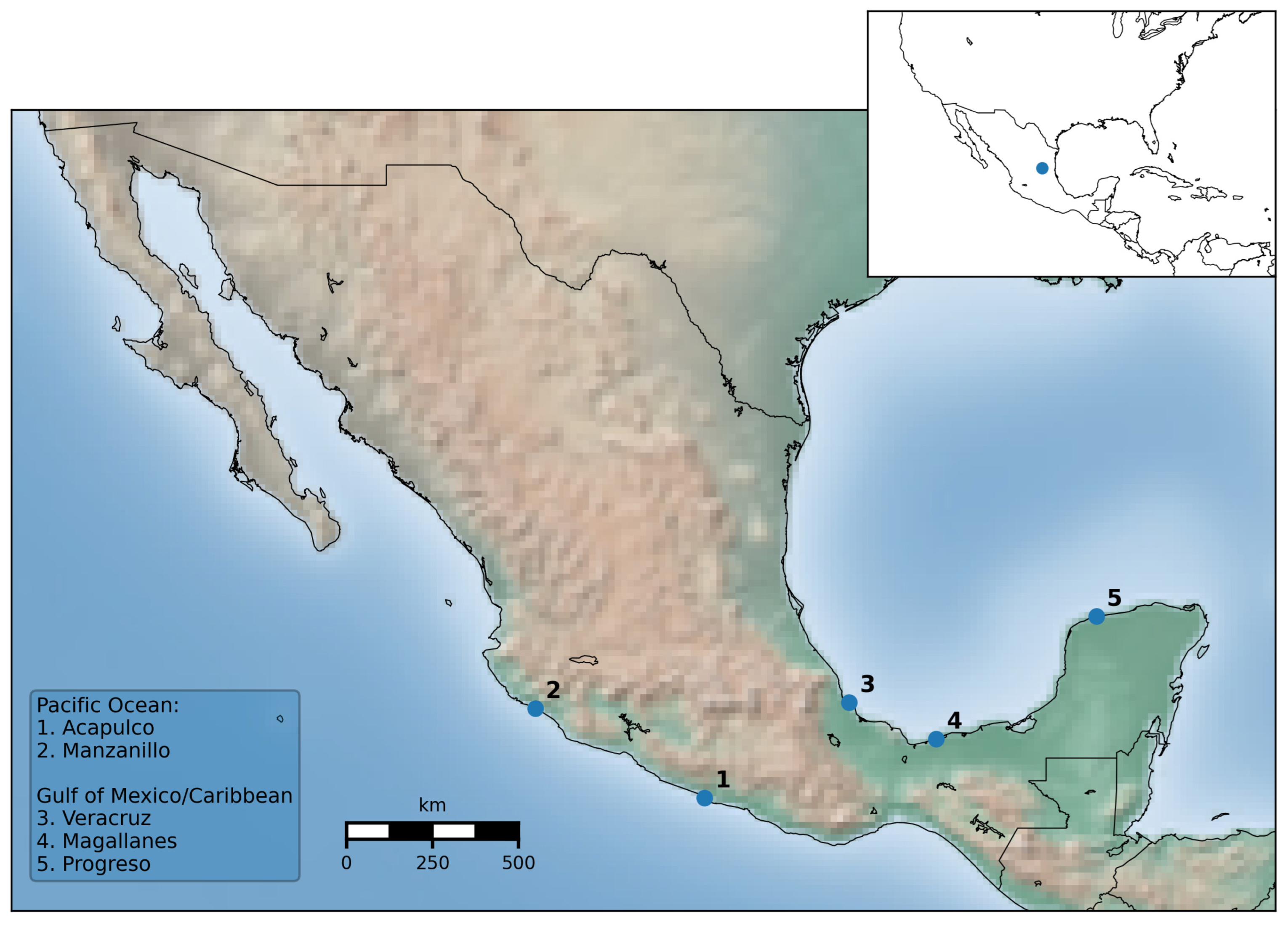
We analyze sea-level records from tide gauges located on the Mexican Pacific and Gulf/Caribbean coasts (Figure 1).

Stations were selected to represent contrasting oceanographic regimes and exposure to tropical cyclones and cold fronts as summarized in

Table 1. Tide-gauge stations operated by the Servicio Mareográfico Nacional (Instituto de Geofísica, UNAM) used in this study. Stations are grouped by coastal region to reflect distinct oceanographic and meteorological forcing regimes.

Station	Region	Location	Lat (°N)/Long (°W)	Period Analyzed	Primary Forcing Regime
Acapulco	Pacific	Acapulco, Guerrero	16°50′16.67″/ 99°54′10.64″	2008–2024	Tropical cyclones and ENSO-related variability
Manzanillo	Pacific	Manzanillo, Colima	19°3′0.00″/ 104°19′12.00″	2017–2025	Tropical cyclones and ENSO-related variability
Veracruz	Gulf of Mexico	Veracruz, Veracruz	19°11′31.49″/ 96°7′24.73″	2012–2025	Mixed: Cyclones and cold fronts
Magallanes	Gulf of Mexico	Magallanes, Tabasco	18°17′48.34″/ 93°51′16.36″	2016–2025	Mixed: Cyclones, cold fronts and fluvial influence
Progreso	Gulf/Caribbean	Progreso, Yucatán	21°18′11.34″/ 89°39′59.32″	2015–2025	Tropical Cyclones and Caribbean circulation patterns

. The dominant physical drivers of extreme sea-level variability differ between regions, motivating the regional comparative framework adopted in this study.

Sea-level records include sub-hourly (e.g., 6 min) and hourly observations and cover multi-year periods depending on data availability. All timestamps were standardized and processed as MATLAB R2025b datetime objects to ensure reproducibility.

Quality control included removal of invalid or missing values (e.g., 9.999), elimination of non-finite records, and homogenization to hourly resolution. No interpolation or imputation was applied. Given the high temporal resolution and the declustering procedure used in the extreme-value analysis, data gaps do not significantly affect the identification of independent extreme events.

Let η(t) denote the observed sea level (m). The mean sea level over the analysis period is computed as MSL = mean(η), and the centered series is

η₀(t) = η(t) − MSL.

(1)

where η₀(t) is the centered sea-level series, and MSL is the mean sea level.

The astronomical tide η_astr(t) is estimated via classical harmonic analysis using the T_TIDE toolbox [17]. To reduce computational cost for long records while preserving constituent stability, the harmonic fit is performed on a representative multi-year subset (typically 2–3 years) and with linear error estimates (bootstrap disabled). The fitted harmonic constituents are then synthesized over the full record using the corresponding synthesis routine. The meteorological residual (storm-surge component) is computed as

η_met(t) = η₀(t) − η_astr(t).

(2)

where η_met(t) is storm-surge component.

Monthly maxima are extracted from η_met(t) using a calendar-month aggregation:

Y__m = max{η__met(t)} t in month m. The resulting monthly maxima time series is retained in chronological order (vector Y) along with its time vector (Julian date T) for EVT fitting. To diagnose seasonality, maxima are also arranged into a 12-column matrix (Jan–Dec), where each column pools all maxima from the corresponding calendar month across years. The 95th percentile was computed with monthly maxima as a robust upper-tail diagnostic, and the seasonal structure was visualized using compact boxplots with cyclone-season shading.

Cyclone-season months are defined as May–November for the Pacific and June–November for the Gulf/Caribbean. Monthly maxima are partitioned into cyclone-season and non-cyclone-season subsets to assess seasonal modulation of extremes.

ENSO-phase stratification is included to assess interannual climate modulation of extreme sea levels and to provide a basis for future non-stationary extreme-value modeling.

ENSO phases are assigned using the Oceanic Niño Index (ONI). The ONI data file is converted into a monthly datetime series by mapping each 3-month season (DJF, JFM, …, NDJ) to its central month (January, February, …, December). Monthly maxima are matched by year–month to ONI values and classified as El Niño (ONI ≥ 0.5), La Niña (ONI ≤ −0.5), or Neutral (|ONI| < 0.5).

2.2. Extreme-Value Analysis Framework

Extreme sea-level events are rare and occur in the upper tail of the distribution. Extreme-value theory (EVT) provides a consistent framework and has been widely applied in coastal engineering for the estimation of design water levels [18], for modeling such events, and for estimating return levels relevant for coastal risk assessment [7].

In this study, two complementary EVT approaches are applied: a block maxima approach (GEV) used for seasonal characterization and a Peaks-Over-Threshold (POT–GPD) approach, adopted as the primary framework for extreme-value estimation. This dual approach allows for separating temporal variability from tail behavior while ensuring robust estimation of extremes.

2.2.1. Generalized Extreme Value (GEV) Model

Under the block maxima approach, the maximum value within each block of observations is assumed to follow a Generalized Extreme Value (GEV) distribution. Here, blocks are defined monthly to preserve seasonal information while ensuring sufficient sample size for statistical inference. In this study, blocks are defined at a monthly scale to preserve seasonal variability while maintaining sufficient sample size. The GEV distribution arises as the asymptotic distribution of normalized maxima of independent and identically distributed random variables and is defined by three parameters: location (μ), scale (σ > 0), and shape (ξ).

The cumulative distribution function of the GEV distribution is given by Equation (3):

$$G\left(z\right)=\exp \left\{{\left[1+\xi \left({\displaystyle \frac{z-\mu }{\sigma }}\right)\right]}^{-{\displaystyle \frac{1}{\xi }}}\right\}, \mathrm{for}1+\xi \left({\displaystyle \frac{z-\mu }{\sigma }}\right)>0$$

(3)

where the shape parameter ξ governs the tail behavior of the distribution and is of particular importance for coastal hazard assessment. Positive values of ξ correspond to heavy-tailed (Fréchet-type) behavior, ξ ≈ 0 represents the Gumbel case with exponentially decaying tails, and negative ξ implies a bounded upper tail (Weibull-type). Consequently, regional differences in ξ provide insight into the physical mechanisms controlling extreme sea levels and the potential severity of rare events. The GEV model is used here to characterize seasonal variability and provide consistent regional comparisons.

Return levels corresponding to a return period (Tr) are estimated from the inverse GEV distribution and represent the magnitude expected to be exceeded with an average annual exceedance probability of 1/Tr. These estimates are widely used as design criteria in coastal engineering and risk assessment.

2.2.2. Peaks-Over-Threshold (POT) and Generalized Pareto Distribution (GPD) Model

To robustly characterize extreme sea levels, a Peaks-Over-Threshold (POT) approach is applied directly to the continuous hourly residual series. Threshold selection was further supported by the stability of GPD parameters and return levels across the selected percentile range.

In this approach, all sea-level residuals exceeding a sufficiently high threshold $\left(u\right)$ are considered, allowing for a more efficient use of available data, particularly for the estimation of long return periods. A high threshold (u) was selected using percentile criteria (99.0–99.5%) and validated through sensitivity analysis, ensuring stable parameter estimates and return levels. To ensure approximate independence of exceedances, a temporal declustering procedure was applied using a 72 h window. Only the maximum value within each cluster was retained as an independent event.

Exceedances $y=z-u$, conditional on $z>u$, are modeled using the Generalized Pareto Distribution (GPD), whose cumulative distribution function is given by Equation (4):

$$H\left(y\right)=1-{\left(1+\xi {\displaystyle \frac{y}{\beta }}\right)}^{-{\displaystyle \frac{1}{\xi }}}, \mathrm{for}y>0$$

(4)

where β > 0 is the scale parameter, and ξ is the shape parameter, consistent with the GEV formulation. The occurrence of independent exceedances is modeled as a Poisson process with rate λ (events per year), leading to a combined Poisson–Generalized Pareto (PP–GPD) model for extreme sea levels.

Return levels are derived from the combined Poisson–GPD model. Parameter uncertainty and confidence intervals are estimated using bootstrap resampling.

Given the relatively short record lengths, return periods up to approximately 25 years are considered the most robust, while longer return periods (50–100 years) are treated as exploratory estimates.

2.2.3. Positioning Within Coastal Hazard Frameworks

Extreme sea-level analysis has evolved toward probabilistic frameworks integrating storm surge, waves, tide (e.g., Joint Probability Method [19,20]), and large-scale systems such as the FEMA–USACE Coastal Hazard System [21]. These approaches explicitly address mixed storm populations and dependence structures [22,23,24]. In contrast, this study adopts a univariate EVT framework to explore regional variability in extreme sea levels. While simpler, this approach provides physically interpretable results and allows for the identification of differences in tail behavior across regions.

3. Results

3.1. De-Tiding Performance and Residual Characteristics

Harmonic analysis successfully isolates the astronomical tide and yields a meteorological residual that concentrates non-tidal variability. The residual exhibits intermittent peaks associated with energetic atmospheric forcing. For long records, linear error estimation is used to ensure computational efficiency while preserving constituent stability. Residual time series are retained for monthly maxima extraction and EVT fitting.

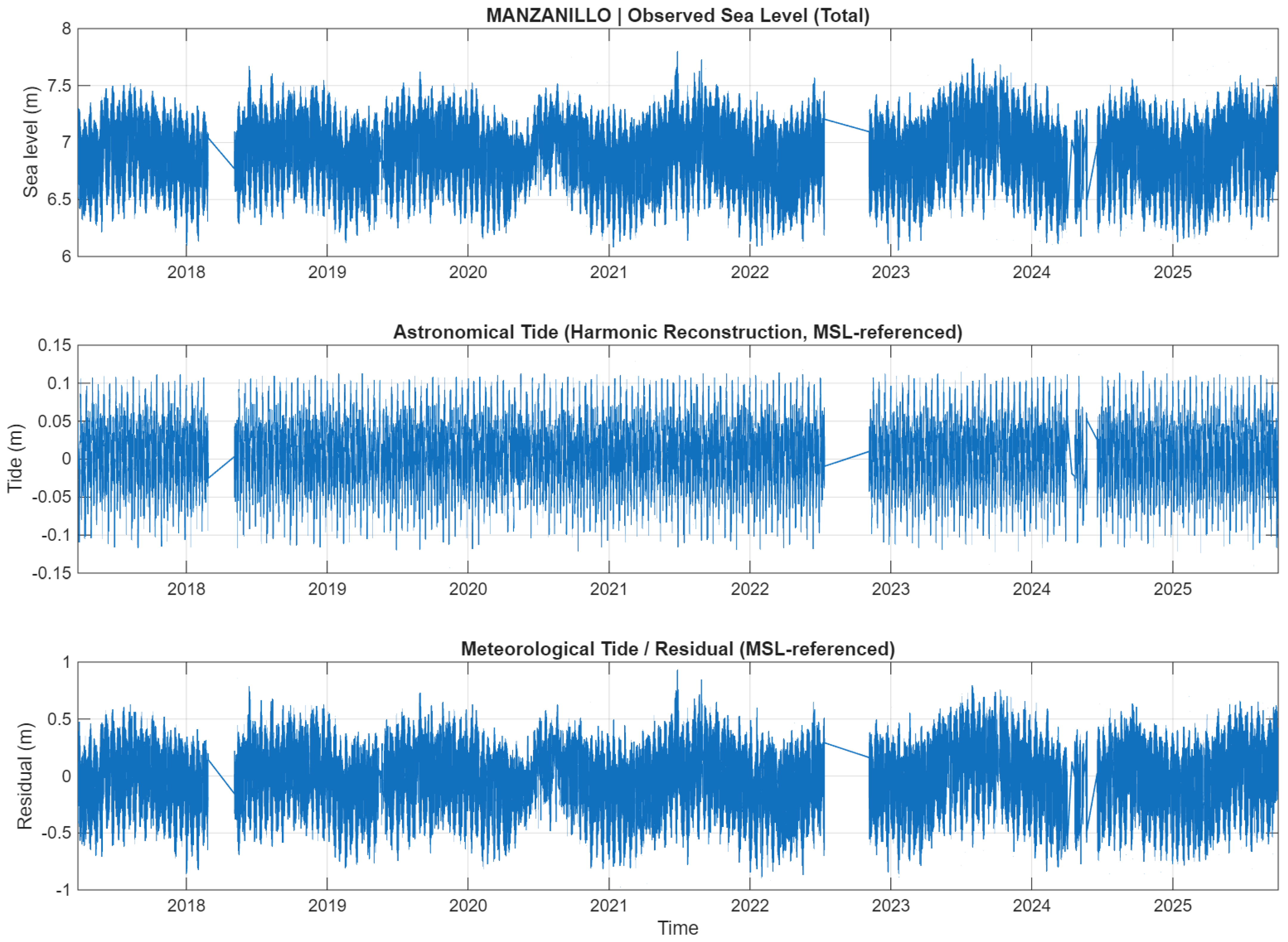
The de-tiding procedure allows for the separation of the observed sea-level signal into its main physical components. Figure 2 illustrates this decomposition for the Manzanillo tide-gauge record.

The upper panel shows the observed sea level, which includes tidal variability, mean sea-level variations, and meteorological contributions. The middle panel presents the astronomical tide reconstructed through harmonic analysis using the main tidal constituents. Subtracting this component from the observed record yields the meteorological residual (lower panel), which represents non-tidal sea-level variability associated with atmospheric forcing such as storm surges, wind setup, and large-scale ocean–atmosphere interactions. The residual series exhibits intermittent peaks linked to energetic atmospheric forcing and provides the basis for both the seasonal diagnostics and the extreme-value analysis presented in the following sections.

3.2. Seasonal Variability of Monthly Maxima

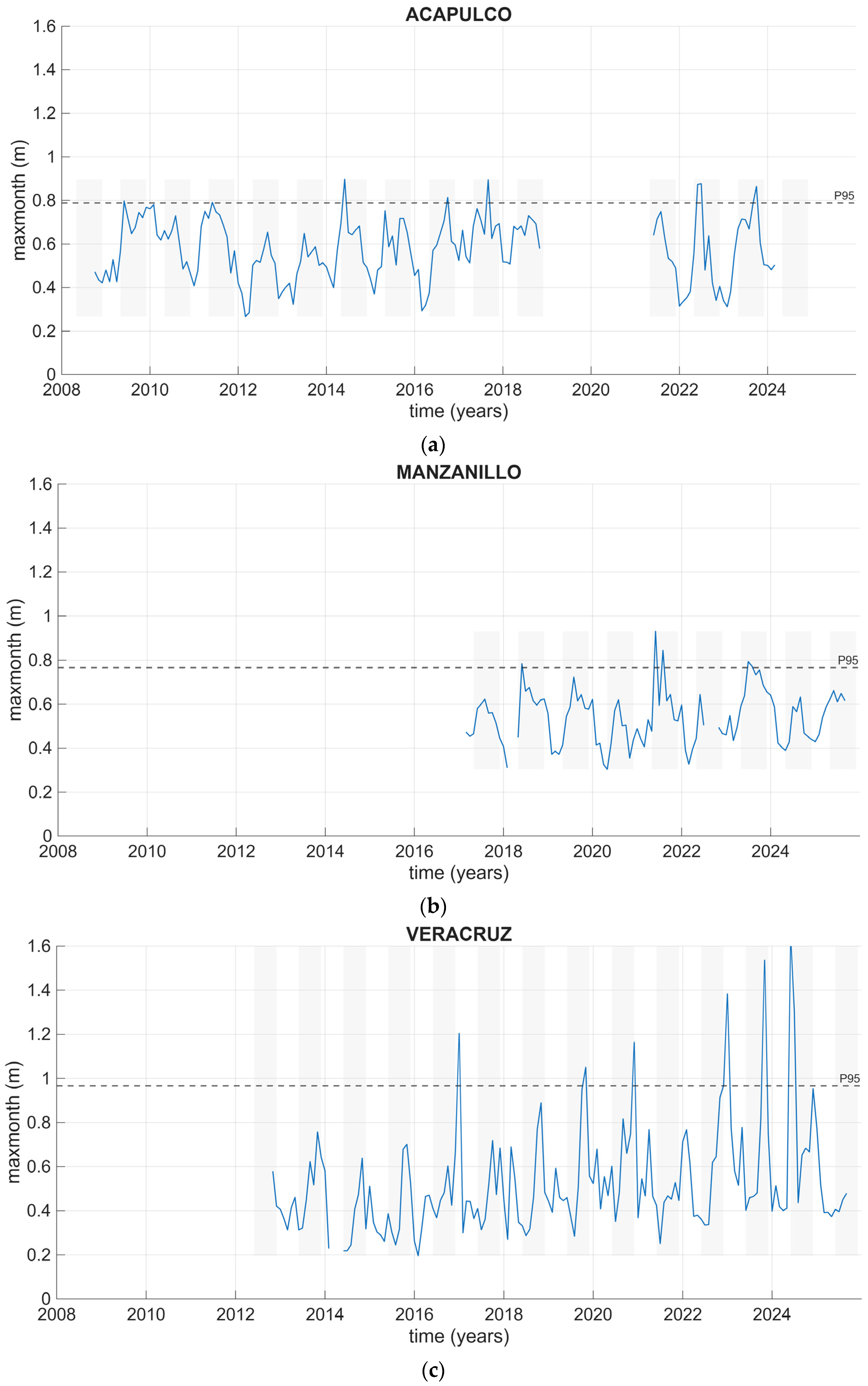
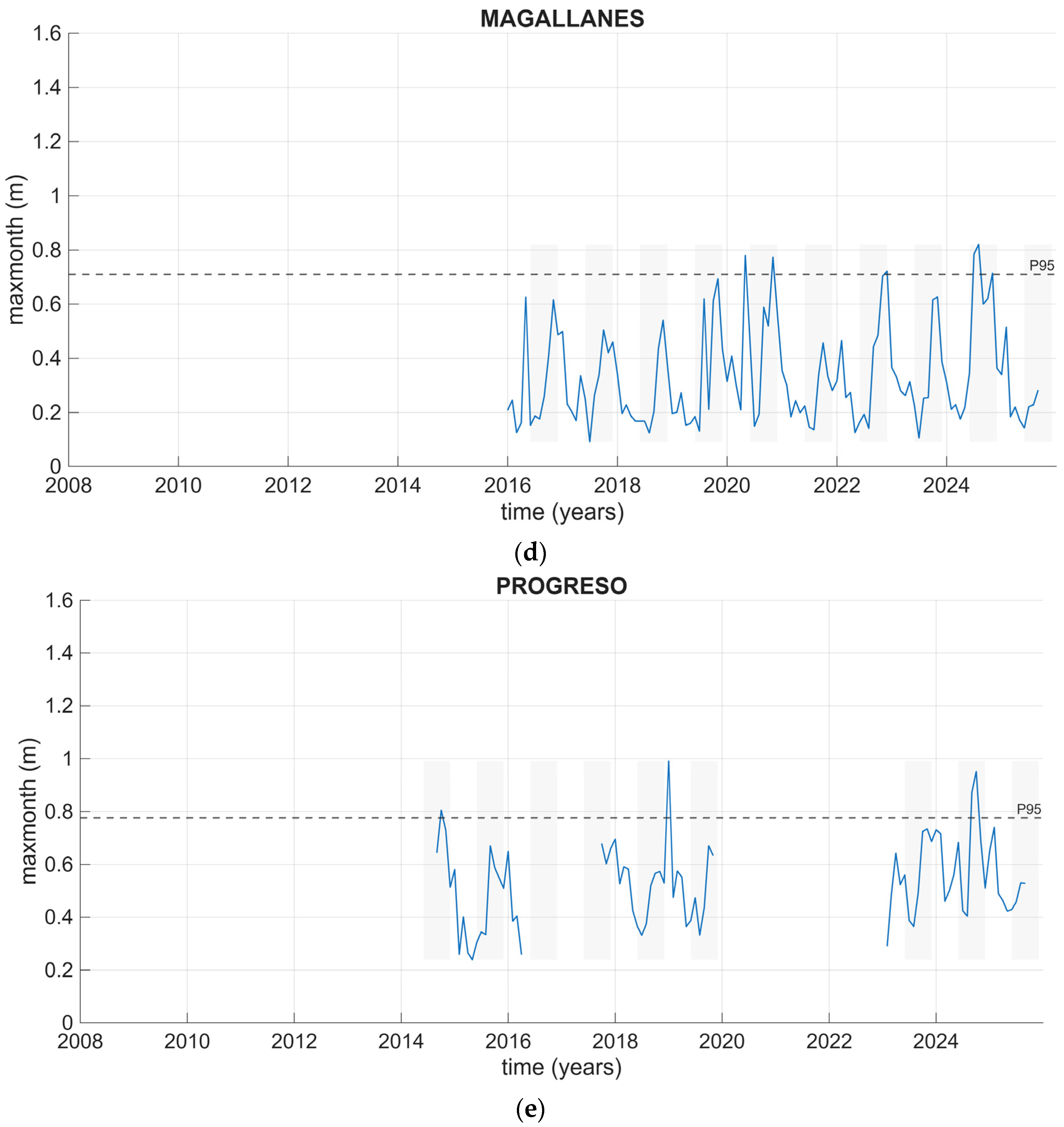
Monthly maxima of the meteorological residual reveal a clear modulation by the cyclone season at all stations, although the magnitude and persistence of this modulation differ between the Pacific and the Gulf of Mexico–Caribbean regions. Figure 3 shows the time series of monthly maxima, with shaded intervals indicating the cyclone season and the dashed line representing the 95th percentile (P95). Several extreme outliers exceed the 95th percentile threshold, particularly during the cyclone season. These apparent outliers correspond to physically meaningful extreme events associated with intense meteorological forcing (e.g., tropical cyclones or cold fronts). They are therefore retained in the analysis, as they represent the upper tail of the distribution and are essential for extreme-value modeling.

At all stations, most of the largest monthly maxima occur during the cyclone season, confirming the importance of tropical forcing in shaping the upper part of the distribution. However, the Gulf of Mexico stations, especially Veracruz, also show elevated values outside the cyclone season, indicating that additional meteorological processes, particularly strong cold fronts (“nortes”), contribute to extreme water-level anomalies.

Veracruz exhibits the highest absolute monthly maxima among the analyzed stations, with several values exceeding 1.5 m and a P95 close to 0.97 m. These peaks occur mainly during the cyclone season but are not restricted to it, suggesting the combined influence of tropical cyclones and extratropical atmospheric forcing. In contrast, Pacific stations display a more concentrated seasonal structure, with the largest extremes clustered during the tropical cyclone months.

These results indicate that seasonality is a first-order control on extreme sea-level variability, but its expression differs substantially between coasts.

3.3. Monthly Distributions and Regional Seasonal Contrast

3.3.1. Pacific Coast Stations

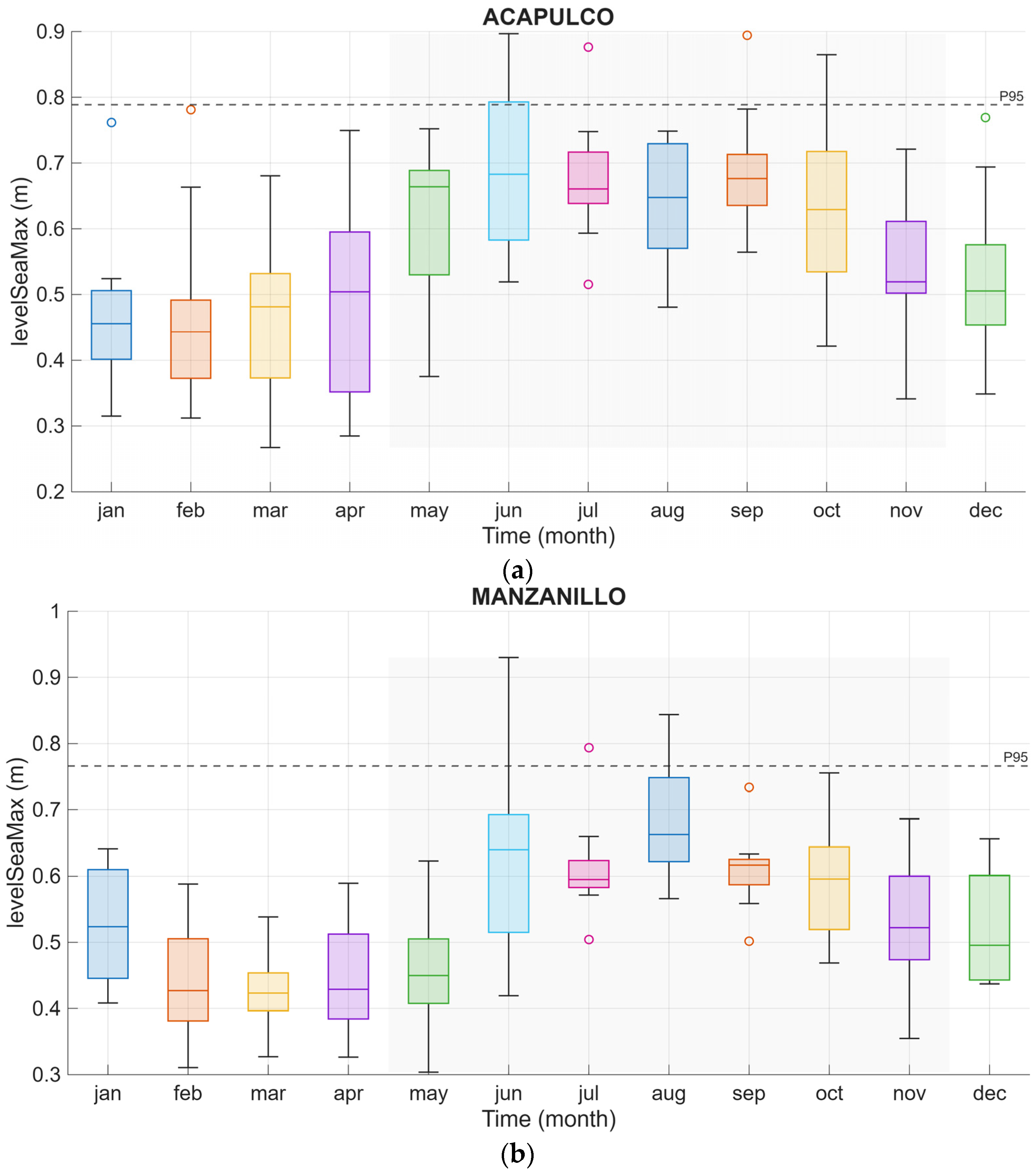
Acapulco and Manzanillo exhibit pronounced seasonal modulation of monthly maxima (Figure 4). In both stations, the cyclone season contains most of the highest values and the widest monthly distributions. At Acapulco, 92 out of 156 monthly maxima occur during the cyclone season (May–November). The overall P95 is 0.788 m, increasing to 0.859 m during the cyclone season and decreasing to 0.753 m outside it. The monthly distributions show enhanced dispersion in late spring and early summer, indicating that elevated water levels can occur both at the onset and during the core of the tropical cyclone season. Manzanillo shows a stronger seasonal amplification. Of the 98 monthly maxima, 58 occur during the cyclone season. The P95 increases from 0.632 m outside the cyclone season to 0.790 m during it, with an overall P95 of 0.766 m. June displays the largest spread and the highest extremes, consistent with the early intensification of tropical cyclone activity in the central Mexican Pacific.

Overall, the Pacific coast is characterized by a marked seasonal concentration of extremes, with monthly maxima strongly clustered during cyclone-season months.

3.3.2. Gulf of Mexico and Caribbean Stations

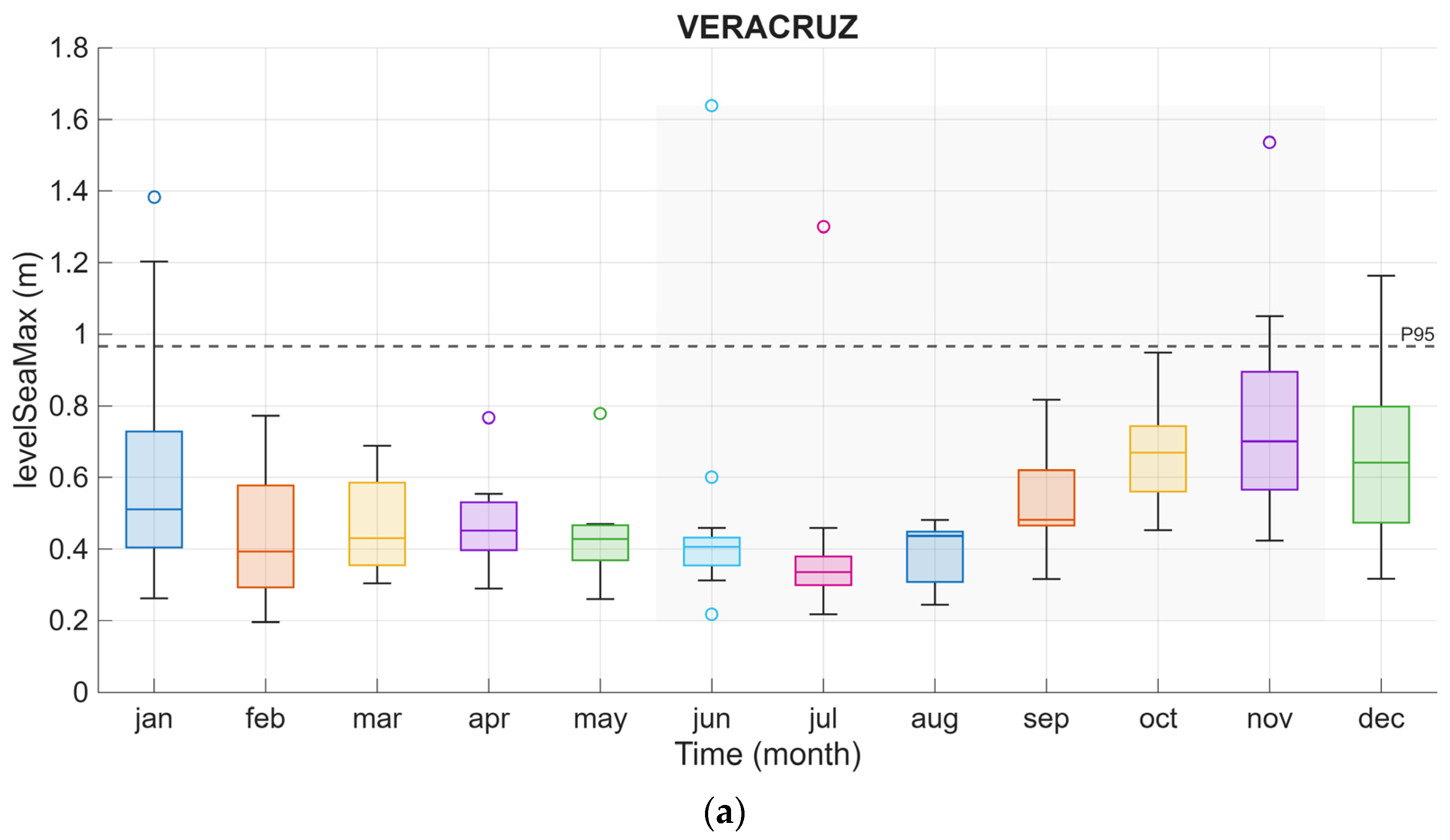
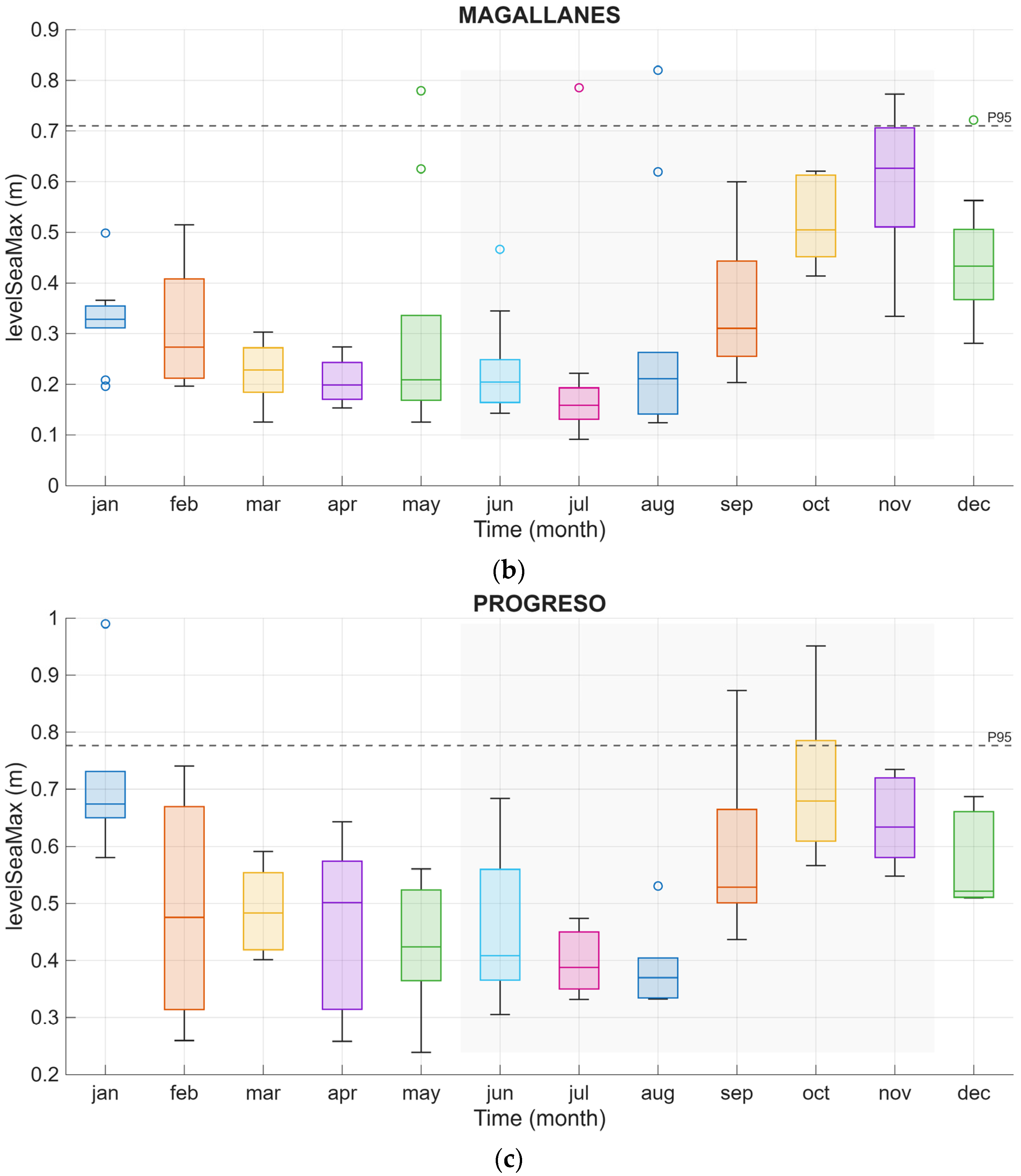
Seasonal modulation is also evident in Veracruz, Magallanes, and Progreso, but the Gulf/Caribbean stations display a broader seasonal window and, in some cases, higher absolute extremes (Figure 5).

Veracruz presents the largest monthly maxima in the dataset. Of the 152 monthly maxima, 77 occur during the cyclone season. The overall P95 is 0.966 m, increasing to 1.010 m during the cyclone season, while remaining nearly unchanged outside it (0.964 m). This weak contrast in seasonal P95, combined with the presence of high values in both warm and cool months, indicates that Veracruz extremes are not controlled exclusively by tropical cyclones. Outlying values in the monthly boxplots correspond to physically meaningful extreme events associated with intense meteorological forcing and were retained because they represent the upper tail of the distribution.

Magallanes shows a more balanced distribution of extremes between seasons, with 59 cyclone-season and 59 non-cyclone-season monthly maxima. The P95 rises from 0.597 m outside the cyclone season to 0.746 m during it, with an overall P95 of 0.710 m. The largest values occur mainly from September to November, indicating strong seasonal control despite the shorter record and lower event frequency.

Progreso shows intermediate behavior. Of the 80 monthly maxima, 41 occur during the cyclone season. The P95 increases from 0.736 m in non-cyclone months to 0.836 m during the cyclone season, with an overall P95 of 0.773 m. Higher medians and wider spreads are concentrated in September–November, although isolated high values also occur outside the cyclone season, suggesting that both tropical cyclones and strong cold fronts contribute to the upper tail.

Taken together, the Gulf of Mexico–Caribbean stations exhibit higher variability and a broader seasonal influence than the Pacific stations, especially at Veracruz.

3.4. Extreme-Value Analysis

3.4.1. GEV Results Based on Monthly Maxima

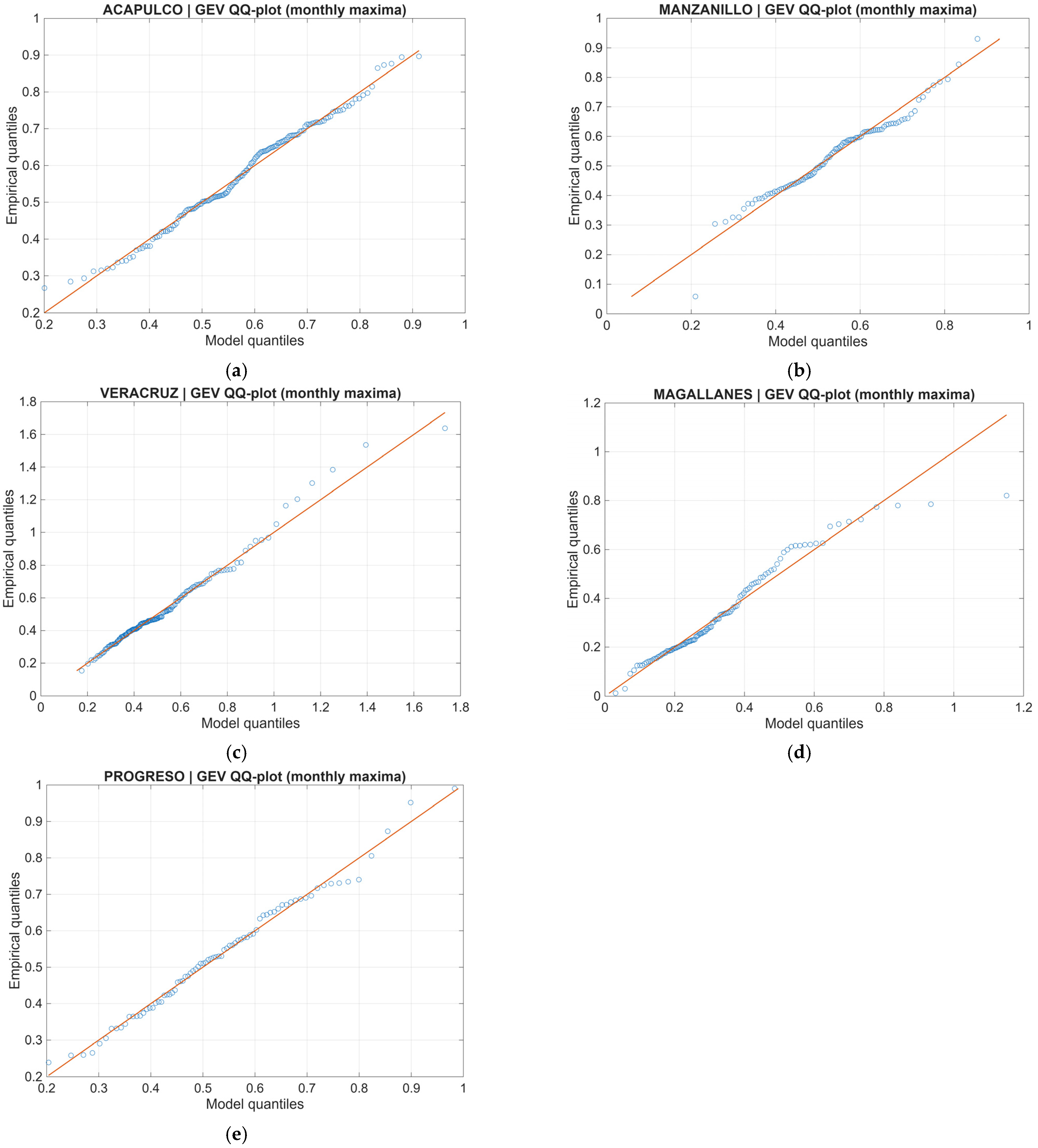
The Generalized Extreme Value (GEV) analysis applied to monthly maxima provides a consistent regional framework for comparing seasonal-scale extremes across stations. The fitted GEV parameters are summarized in

Table 2. Generalized Extreme Value (GEV) parameters estimated from monthly maxima of the meteorological residual at each tide-gauge station.

Station	μ (m)	σ (m)	ξ (–)	Interpretation
Acapulco	0.546	0.138	−0.352	Bounded tail
Manzanillo	0.488	0.134	−0.254	Weakly bounded tail
Veracruz	0.413	0.153	+0.136	Heavy-tail tendency
Progreso	0.461	0.180	−0.281	Weakly bounded tail
Magallanes	0.241	0.150	−0.021	Near-Gumbel

, and model adequacy is evaluated using QQ plots in Figure 6.

The GEV results indicate substantial regional variability in tail behavior. Pacific stations show negative shape parameters, consistent with bounded or weakly bounded tails, whereas Veracruz is the only station with a positive shape parameter, suggesting a tendency toward heavier-tailed behavior. Progreso and Magallanes occupy intermediate positions, with Progreso remaining weakly bounded and Magallanes close to Gumbel conditions. These results support the interpretation that monthly scale extremes differ systematically between the Pacific and Gulf/Caribbean coasts and justify the use of a more detailed threshold-based approach for event-scale analysis.

Across stations, the QQ plots show a satisfactory fit between empirical and modeled quantiles, with only minor deviations at the highest quantiles. These departures are more evident in Gulf/Caribbean stations and likely reflect natural upper-tail variability rather than systematic model failure.

3.4.2. POT–GPD Results from the Continuous Residual Series

The primary extreme-value estimates were obtained using the classical POT approach applied directly to the continuous hourly residual series. Threshold exceedances were declustered using a 72 h window to obtain approximately independent events, and the resulting excesses were modeled using the GPD. Return levels were estimated from the combined Poisson–GPD model, with bootstrap confidence intervals.

Table 3. POT–GPD parameters and selected return levels of extreme sea-level residuals.

Station	Independent Events	λ (Events/Year)	ξ	β (m)	Tr10 (m)	Tr25 (m)	Tr50 (m)	Tr100 (m)
Acapulco	125	8.09	−0.300	0.120	0.872	0.898	0.913	0.926
Manzanillo	84	9.86	−0.183	0.107	0.860	0.899	0.925	0.947
Veracruz	112	8.69	+0.132	0.157	1.443	1.718	1.950	2.204
Magallanes	32	3.30	−0.686	0.232	0.799	0.813	0.819	0.823
Progreso	46	4.11	−0.078	0.105	0.909	0.978	1.027	1.074

summarizes the POT–GPD results for the five stations.

The POT results confirm the regional contrasts suggested by the GEV analysis, but provide a clearer characterization of event-scale extremes.

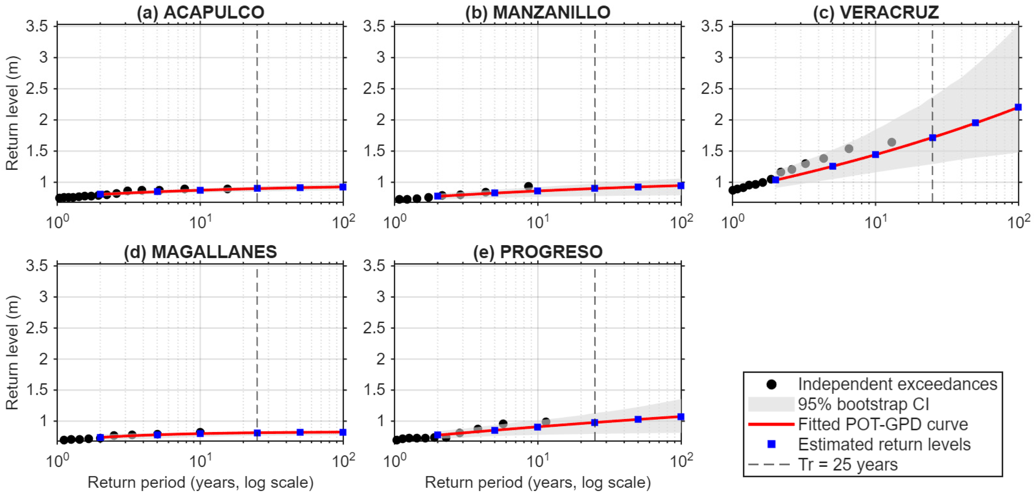
To further illustrate the behavior of extreme sea levels derived from the POT framework, Figure 7 presents the return-level curves estimated from the Poisson–GPD model for all analyzed stations. Solid lines represent the estimated return levels, while shaded areas indicate the 95% bootstrap confidence intervals.

The figure provides a direct visualization of regional differences in tail behavior and uncertainty. In particular, it highlights the contrast between Pacific stations, which exhibit bounded or near-Gumbel behavior with relatively stable return levels, and Gulf of Mexico–Caribbean stations, where return levels increase more rapidly, and uncertainty becomes significantly larger at longer return periods.

As shown in Figure 7, the POT-based return levels confirm the regional contrasts suggested by the GEV analysis, while providing a more robust characterization of event-scale extremes.

Acapulco shows a clearly bounded tail ($\xi =-0.300$), with stable return levels and relatively narrow intervals of uncertainty, reflecting its longer record and larger number of independent events. Manzanillo exhibits weakly bounded to near-Gumbel behavior, with threshold sensitivity tests showing stable return levels across thresholds between the 99.0th and 99.5th percentiles. In particular, the 10-year return level remains close to 0.86 m and the 25-year return level near 0.90 m, indicating robust tail estimation.

Veracruz differs markedly from all other stations. Its positive shape parameter ($\xi =0.132$) indicates a tendency toward heavy-tailed behavior, and return levels increase rapidly with return period, reaching 1.72 m at Tr25 and 2.20 m at Tr100. Confidence intervals also widen substantially at long return periods, highlighting the greater extrapolation uncertainty associated with heavier tails.

Magallanes exhibits the most strongly bounded tail ($\xi =-0.686$), with return levels increasing only marginally beyond Tr10. This suggests a highly constrained upper-tail regime. Progreso remains close to Gumbel behavior ($\xi =-0.078$), with moderate return-level growth and broader uncertainty than Acapulco.

Because record lengths remain limited at several stations, the 25-year return period is adopted as the main basis for inter-station comparison. Longer return periods (50–100 years) are reported for completeness but should be interpreted as exploratory estimates. Because record lengths remain limited at several stations, return levels up to approximately 25 years are considered the most robust for inter-station comparison. As shown in Figure 7, uncertainty increases substantially beyond this range, particularly for stations with heavier tail behavior such as Veracruz. Therefore, return periods of 50 and 100 years are included for completeness but should be interpreted as exploratory estimates rather than definitive design values.

3.4.3. Threshold Sensitivity and Seasonal POT Behavior

Sensitivity tests performed using thresholds between the 99.0th and 99.5th percentiles indicate that GPD parameters vary smoothly and that return levels remain stable across the selected threshold range. For example, in Manzanillo, the estimated 10-year return level remains close to 0.86 m, and the 25-year return level ranges only from approximately 0.90 to 0.93 m. This confirms that the revised POT estimates are not strongly dependent on a single threshold choice.

Seasonal POT analysis also supports the regional interpretation. In Pacific stations, cyclone-season and non-cyclone-season exceedances generally remain bounded or near-Gumbel. In Veracruz, both seasons show positive shape parameters, suggesting that both tropical and non-tropical forcing contribute to the heavier-tailed behavior. In Progreso, both seasonal subsets remain close to Gumbel conditions, indicating that the Gulf region is not statistically uniform.

These results show that, while multiple physical drivers operate at several stations, their statistical expression differs regionally and does not necessarily invalidate a station-based univariate EVT analysis.

3.5. Interannual Variability: ENSO and Tropical Cyclones

Interannual climate variability in the Pacific basin is strongly influenced by the El Niño–Southern Oscillation (ENSO), which modifies atmospheric circulation, sea-surface temperature, and regional ocean dynamics [6]. These large-scale processes can alter background sea levels and influence the conditions under which storm surges and extreme sea levels develop. This analysis is exploratory and not intended as a predictive model.

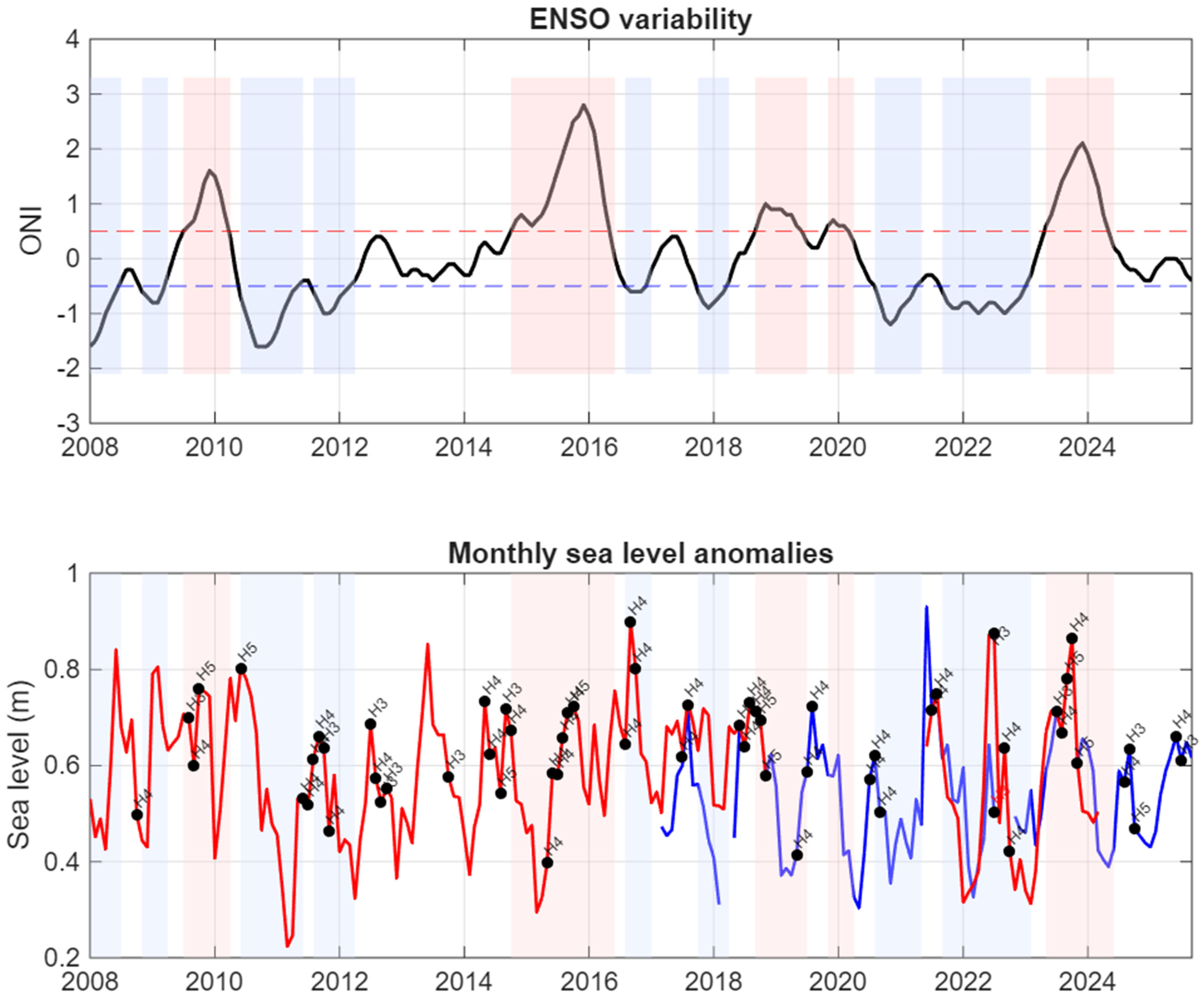
Figure 8 illustrates the temporal evolution of the Oceanic Niño Index (ONI) together with monthly sea-level anomalies observed at the Pacific tide gauges of Manzanillo and Acapulco. ENSO phases were defined using the Oceanic Niño Index (ONI), with thresholds of ±0.5 °C. The upper panel shows the ONI time series, with the conventional thresholds of ±0.5 indicating El Niño and La Niña conditions. The lower panel displays the monthly sea-level anomalies for both stations, with Manzanillo represented in blue and Acapulco in red. The shaded ENSO phases are replicated in this panel to facilitate the comparison between large-scale climatic variability and coastal sea-level responses. Additionally, the occurrence of tropical cyclones is marked with symbols and labels corresponding to the hurricane level on the dates of occurrence. This representation allows the simultaneous visualization of ENSO variability, regional sea-level anomalies, and tropical cyclone activity along the Mexican Pacific coast. The figure suggests that several sea-level peaks coincide with hurricane events, while broader interannual variations appear to be modulated by ENSO conditions. Overall, the combined visualization highlights the interaction between large-scale climate forcing and extreme meteorological events in shaping sea-level variability in the region.

Several of the largest monthly sea-level anomalies coincide with the occurrence of tropical cyclones, while broader interannual fluctuations appear to follow ENSO variability.

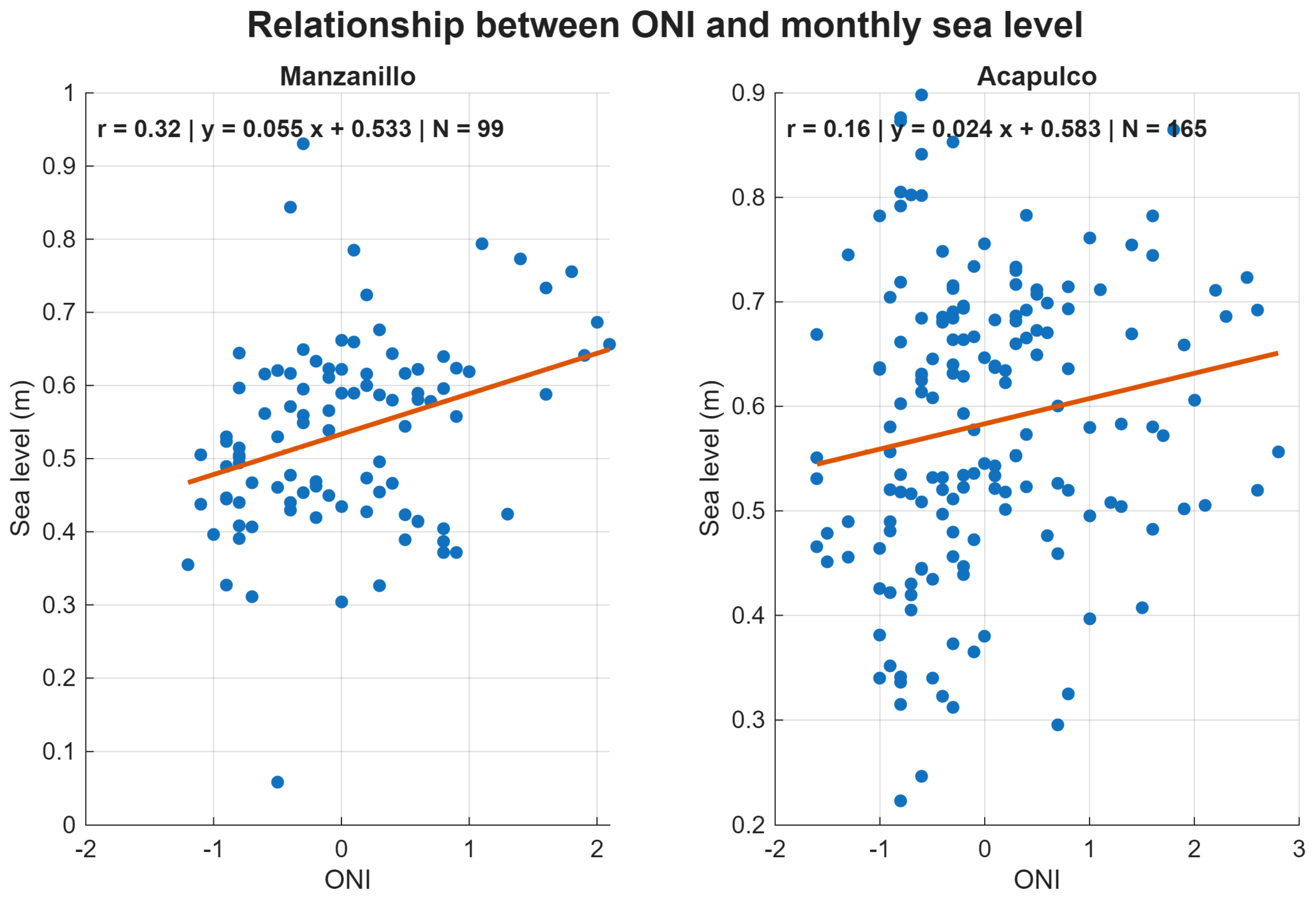
To explore the potential influence of interannual climate variability on extreme sea levels, the relationship between the Oceanic Niño Index (ONI) and monthly sea-level anomalies was examined for the Pacific stations of Manzanillo and Acapulco. Figure 9 presents scatter plots of ONI values against monthly sea levels, together with linear regression fits and Pearson correlation coefficients. The results indicate substantial dispersion and relatively weak linear correlations, suggesting that ENSO does not exert a deterministic control on sea-level variability at these locations.

Although slight tendencies can be observed during some ENSO phases, the broad spread of the data indicates that other regional processes—such as local wind forcing, mesoscale ocean variability, and storm activity—play a significant role in determining monthly sea-level fluctuations. These results are consistent with the interpretation that ENSO primarily modulates background oceanic conditions rather than directly controlling individual extreme sea-level events.

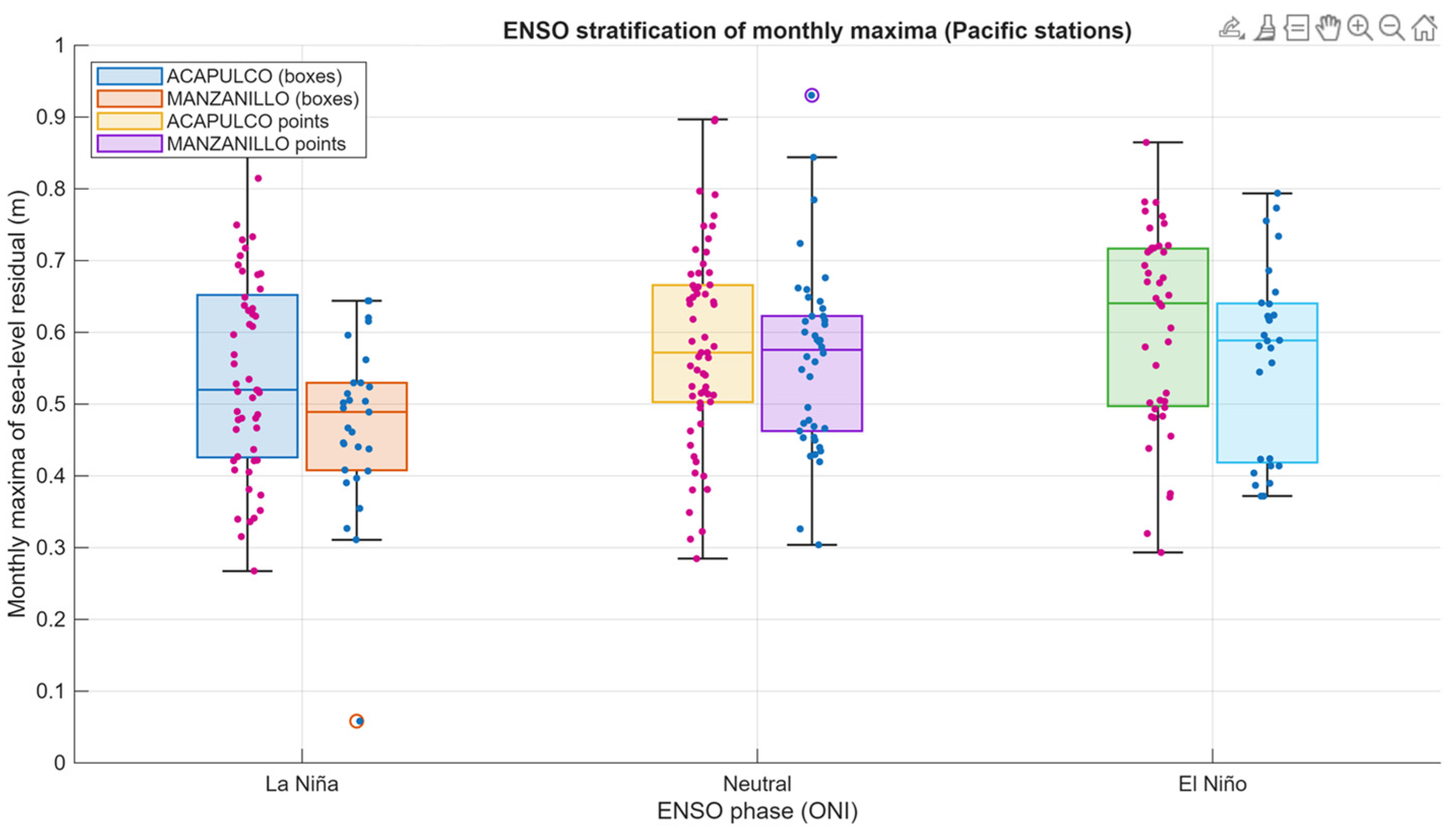
To further investigate the potential ENSO influence, sea-level distributions were stratified according to ENSO phase (La Niña, Neutral, and El Niño), as shown in Figure 10. The boxplots reveal modest shifts in median and interquartile ranges between phases, particularly at the Pacific stations. However, substantial overlap between distributions indicates that extreme sea-level values can occur under all ENSO conditions.

4. Discussion

4.1. Regional Contrast and Seasonal Implications

The results reveal a clear regional contrast in extreme sea-level behavior along the Mexican coasts, which has also been documented in other coastal regions where climatic variability and local forcing lead to distinct regional responses [25], but the results also show substantial variability within each basin. Pacific stations exhibit a pronounced seasonal modulation, with most of the highest residuals concentrated during the tropical cyclone season. However, the statistical expression of the upper tail is not uniform across the Pacific. Acapulco shows a clearly bounded tail, Manzanillo exhibits weakly bounded to near-Gumbel behavior, and Magallanes displays the most strongly bounded tail of all analyzed stations. This indicates that, although tropical cyclone forcing is the dominant seasonal control in the Pacific, the resulting extreme-value behavior still varies from station to station. In contrast, the Gulf of Mexico–Caribbean stations display a broader seasonal footprint and, in some cases, higher absolute extremes. Veracruz stands out as the station with the largest return levels and the clearest tendency toward heavy-tailed behavior, while Progreso remains closer to Gumbel conditions. This difference suggests that the Gulf of Mexico–Caribbean region cannot be treated as statistically uniform. Instead, the regional signal reflects local combinations of tropical cyclones, cold fronts, and coastal-oceanographic settings. These patterns support the use of regionally informed interpretations of coastal hazards. From a physical standpoint, the Pacific stations are characterized by a narrower seasonal concentration of extremes, whereas Veracruz in particular reflects the combined contribution of tropical and extratropical forcing over a broader annual window. Consequently, the Mexican coasts are better described as a set of distinct extreme-value regimes rather than a single national-scale statistical system. The seasonal analysis further reinforces this interpretation. In the Pacific, cyclone-season and non-cyclone-season exceedances generally remain bounded or near-Gumbel, whereas in Veracruz, both seasonal subsets show positive shape parameters, suggesting that heavy-tail tendencies are not confined to tropical cyclone months alone. This indicates that seasonality is fundamental, but it interacts with local forcing conditions in different ways across stations.

4.2. Complementary Roles of the GEV and POT Frameworks

A key outcome of the revised analysis is that the GEV and POT approaches provide complementary, rather than competing, perspectives on extreme sea-level behavior. The GEV model, applied to monthly maxima, is useful for capturing seasonal-scale variability and providing a consistent regional comparison of monthly extremes. In contrast, the POT–GPD approach, applied directly to the continuous residual series with temporal declustering, provides a more physically consistent representation of event-scale extremes and is therefore adopted here as the primary basis for return-level estimation.

The consistency between the two frameworks is strongest at the level of regional pattern recognition, as recent studies highlight the increasing use of hybrid and data-rich approaches for extreme sea-level estimation [14]. Both approaches identify bounded or near-Gumbel behavior at Pacific stations and a heavier-tailed tendency at Veracruz. This convergence is important because it indicates that the main geographical contrasts are not an artifact of a single modeling approach. At the same time, the two methods are not expected to produce identical numerical return levels, since they use different subsets of information: monthly block maxima in the GEV case and threshold exceedances in the POT case.

For this reason, the POT results are given greater weight in the interpretation of return levels. Because the POT framework exploits a larger fraction of the extreme information in the continuous record and explicitly separates exceedance magnitude from event frequency, it provides a stronger basis for event-scale hazard characterization. The GEV results remain useful as a contextual reference, particularly for seasonal-scale interpretation, but should not be viewed as the primary basis for extrapolation to long return periods.

This distinction is especially relevant at stations with contrasting tail behavior. At Veracruz, the positive POT shape parameter and the rapid increase in return levels with recurrence interval are physically consistent with a broader and less constrained upper tail. At Magallanes, the strongly negative POT shape parameter and the near-saturation of return levels beyond Tr10 indicate a highly bounded regime. These differences confirm that a single interpretation of tail behavior is not appropriate across the Mexican coasts.

4.3. Implications for Extreme-Value Modeling

The results underscore the importance of using flexible EVT frameworks that are able to capture spatial differences in both seasonality and tail behavior. The Pacific stations generally show bounded or near-Gumbel behavior, which implies relatively stable return levels and limited growth in design values at longer recurrence intervals. In contrast, Veracruz shows a tendency toward heavy-tailed behavior, leading to more rapid increases in return levels and substantially wider uncertainty bounds at long return periods.

These differences have direct methodological implications. First, they indicate that a single national extreme-value parameterization is unlikely to represent the diversity of coastal processes acting along the Mexican coast. Second, they show that return-level estimation is highly sensitive to local tail structure. Stations such as Acapulco, with negative and relatively well-constrained shape parameters, support more stable extrapolation, whereas stations such as Veracruz require more caution because positive shape parameters amplify long-period uncertainty. The seasonal POT results also help address concerns regarding mixed storm populations. Multiple physical drivers operate at several stations, especially in the Gulf of Mexico. However, the seasonal analyses suggest that these processes do not necessarily produce incompatible statistical behavior within each station. In Veracruz, both cyclone-season and non-cyclone-season exceedances remain weakly positive in shape, while in Progreso, both seasonal subsets remain near-Gumbel. This suggests that a station-based univariate EVT framework can still provide meaningful and interpretable results, even when several forcing mechanisms contribute to the observed extremes. At the same time, the findings also point toward the limits of purely stationary single-population models. Future developments should explore seasonally stratified or covariate-dependent formulations, especially in regions where tropical cyclones and cold fronts jointly influence the upper tail. In this sense, the present study should be viewed as a robust first-order characterization of regional extreme-value behavior, rather than as a final probabilistic hazard model.

4.4. Implications for Coastal Design and Risk Management Under Sea-Level Rise

From an engineering and risk-management perspective, the results have direct implications for the definition of design water levels and adaptation strategies. In the Pacific, where tails are bounded or near-Gumbel, and extremes are concentrated in the cyclone season, design criteria should emphasize the seasonal coincidence of elevated water levels with tropical cyclone activity. In these settings, the timing and clustering of events may be as important as the absolute magnitude of individual extremes [26]. In contrast, the Gulf of Mexico—particularly Veracruz—shows larger return levels and a broader seasonal influence, implying that hazard conditions cannot be understood solely through tropical cyclone occurrence. In such settings, design and adaptation strategies must be robust, consistent with recent studies applying combined EVT approaches in coastal environments [27], to uncertainty in extreme-value estimation, as reliability-based approaches have shown that model assumptions can significantly affect coastal risk predictions. The markedly higher Tr25 values at Veracruz compared with Pacific stations illustrate the practical importance of this distinction for coastal infrastructure and flood-risk planning. The role of sea-level rise is especially relevant in this context [16]. Sea-level rise acts as a shifting baseline leading to a nonlinear increase in the frequency of extreme coastal water levels [28] that can effectively reduce the recurrence interval of damaging water levels, even when the statistical properties of storm-driven residuals remain unchanged. Thus, although the present study focuses on present-day residual extremes, the results provide an essential baseline for integrating future mean sea-level changes into flood-hazard assessments, as recent studies indicate evolving extreme sea-level behavior under changing climate conditions [29]. This is particularly important in locations where return levels are already high and where tail behavior suggests the possibility of more extreme outliers. Recent coastal hazard frameworks increasingly emphasize the combined effects of sea-level rise, storm surge, waves, and compound flooding and probabilistic assessments of coastal flooding hazards [30]. While the present study adopts a simpler station-based EVT perspective, the strong regional contrasts identified here show that adaptation strategies in Mexico should not be uniform. Instead, design criteria should reflect local forcing regimes, tail behavior, and uncertainty levels, particularly when long-lived infrastructure is considered.

4.5. ENSO as a Secondary Modulator

The ENSO analysis suggests that ENSO acts primarily as a secondary modulator of background sea-level variability rather than as a deterministic driver of extreme sea-level events at the analyzed Pacific stations. Elevated anomalies occur under El Niño, La Niña, and Neutral conditions, and the substantial overlap among phase-stratified distributions indicates that extremes are not confined to a specific ENSO state. This does not imply that ENSO is irrelevant. Rather, it suggests that ENSO may alter the background conditions under which storm-driven extremes occur, while local storm activity, wind forcing, and mesoscale ocean processes continue to govern the development of individual high-water events. Extreme sea levels occur under all ENSO phases, with the highest anomalies frequently associated with tropical cyclone activity, which has been shown to strongly control extreme sea-level variability in recent studies [26]. Several of the highest anomalies coincide with documented tropical cyclone occurrence, reinforcing the interpretation that short-term extremes are driven primarily by storm forcing, not by ENSO phase alone [31]. From a modeling standpoint, ENSO remains a plausible candidate covariate for future non-stationary analyses, especially in the Pacific. However, the present results support a cautious interpretation: the evidence is consistent with modulation, not deterministic control.

4.6. Limitations and Outlook

Several limitations should be acknowledged. First, record lengths differ substantially across stations, and some of the available series remain short relative to the longest return periods considered. For this reason, return periods up to approximately 25 years are considered the most robust basis for inter-station comparison in this study, while 50- and 100-year return levels are presented only as exploratory estimates. This distinction is particularly important at stations with positive or weakly constrained shape parameters, where uncertainty grows rapidly with extrapolation. Second, the number of independent exceedances varies notably among stations. Acapulco and Veracruz provide relatively rich exceedance samples, whereas Magallanes and Progreso are based on fewer events. This affects the stability of parameter estimation and partly explains the wider uncertainty ranges at some sites. Third, although the declustered POT analysis addresses event independence more explicitly than the original implementation, the present framework remains univariate and station-based. It does not explicitly represent joint wave–surge interactions, mixed-population hazard formulations, or multivariate dependence structures of the type used in more comprehensive probabilistic coastal hazard systems.

Future work should therefore extend the present framework in three directions: implementation of non-stationary EVT models with mean sea level and climate indices as covariates; explicit seasonal or mixed-population formulations in regions where multiple forcing mechanisms shape the upper tail; and integration with broader probabilistic coastal hazard frameworks capable of accounting for compound and multivariate processes.

Despite these limitations, the present study provides a reproducible and physically interpretable baseline for understanding the regional structure of extreme sea levels along the Mexican coasts. Its main contribution lies in showing that both seasonality and tail behavior vary substantially across locations, with direct implications for hazard characterization, design criteria, and climate adaptation planning.

5. Summary and Conclusions

This study presents a comprehensive analysis of extreme sea-level behavior along the Mexican coasts by combining harmonic tidal analysis, seasonal diagnostics, and extreme-value theory. By isolating the meteorological residual from tide-gauge records and modeling its extremes using both Generalized Extreme Value (GEV) and Poisson–Generalized Pareto (PP–GPD) frameworks, the study provides a robust and regionally differentiated characterization of coastal extreme water levels. The results reveal a clear regional contrast between the Pacific and the Gulf of Mexico–Caribbean coasts, together with substantial variability within each basin. Pacific stations exhibit a strong seasonal concentration of extremes during the tropical cyclone season and are generally characterized by bounded or near-Gumbel behavior. In contrast, Gulf and Caribbean stations display higher absolute extremes and a broader seasonal influence. Veracruz, in particular, shows a tendency toward heavier-tailed behavior, reflecting the combined influence of tropical cyclones and cold-front systems.

The comparison between GEV and PP–GPD frameworks, which have been increasingly adopted in recent coastal engineering applications for improved tail characterization, highlights their complementary roles. Both approaches consistently identify regional patterns in extreme sea-level behavior, although they do not necessarily yield identical return-level estimates. The POT–GPD framework is adopted as the primary basis for return-level estimation, as it explicitly represents event-scale extremes and incorporates exceedance frequency. The GEV model remains valuable as a contextual reference for monthly scale variability and seasonal interpretation.

Return-level estimates indicate that periods up to approximately 25 years provide the most robust basis for comparison across stations. In contrast, longer return periods (50–100 years) are associated with increasing uncertainty due to record-length limitations and sensitivity to tail behavior, particularly at stations with positive or weakly constrained shape parameters. From an applied perspective, the results demonstrate that extreme sea-level hazards along the Mexican coasts cannot be treated as spatially uniform or strictly stationary. Seasonality, local forcing mechanisms, and mean sea-level variability jointly modulate the upper tail of sea-level distributions. Incorporating mean sea level as a covariate in extreme-value models, therefore, provides a physically consistent pathway to account for sea-level rise and to translate statistical results into actionable coastal design criteria.

The analysis of ENSO variability further indicates that ENSO acts primarily as a secondary modulator of background sea-level conditions rather than as a deterministic driver of extreme events. This suggests that local atmospheric forcing dominates short-term extremes, while large-scale climate modes contribute to interannual variability.

Overall, the proposed workflow provides a reproducible and adaptable framework for analyzing extreme sea levels in data-rich coastal regions. The results demonstrate that extreme sea levels along the Mexican coasts are governed by region-specific forcing and tail behavior, requiring localized modeling strategies rather than a uniform national approach. These findings have direct implications for coastal engineering design, flood-risk assessment, and climate adaptation planning under ongoing sea-level rise.

References

1. Wahl, T.; Haigh, I.; Nicholls, R.; Arns, A.; Dangendorf, S.; Hinkel, J.; Slangen, A.B.A. Understanding extreme sea levels for broad-scale coastal impact and adaptation analysis. Nat. Commun. 2017, 8, 16075. [Google Scholar] [CrossRef]
2. Vousdoukas, M.I.; Mentaschi, L.; Voukouvalas, E.; Verlaan, M.; Jevrejeva, S.; Jackson, L.P.; Feyen, L. Global probabilistic projections of extreme sea levels show intensification of coastal flood hazard. Nat. Commun. 2024, 9, 2360. [Google Scholar] [CrossRef]
3. Rizzi, J.; Torresan, S.; Zabeo, A.; Critto, A.; Tosoni, A.; Tomasin, A.; Marcomini, A. Assessing storm surge risk under future sea-level rise scenarios: A case study in the North Adriatic coast. J. Coast. Conserv. 2017, 21, 453–471. [Google Scholar] [CrossRef]
4. Woodworth, P.L.; Melet, A.; Marcos, M.; Ray, R.D.; Wöppelmann, G.; Sasaki, Y.N.; Cirano, M.; Hibbert, A.; Huthnance, J.M.; Monserrat, S.; et al. Forcing Factors Affecting Sea Level Changes at the Coast. Surv. Geophys. 2019, 40, 1351–1397. [Google Scholar] [CrossRef]
5. Appendini, C.M.; Torres-Freyermuth, A.; Salles, P.; López-González, J.; Mendoza, E.T. Wave Climate and Trends for the Gulf of Mexico: A 30-Yr Wave Hindcast. J. Clim. 2014, 27, 1619–1632. [Google Scholar] [CrossRef]
6. Philander, S.G. El Niño, La Niña, and the Southern Oscillation; Academic Press: San Diego, CA, USA, 1990; p. 293. [Google Scholar] [CrossRef]
7. Coles, S.G. An Introduction to Statistical Modelling of Extreme Values, 1st ed.; Springer: London, UK, 2001; Volume 4, pp. 1–208. [Google Scholar]
8. Katz, R.; Parlange, M.; Naveau, P. Statistics of extremes in hydrology. Adv. Water Resour. 2002, 25, 1287–1304. [Google Scholar] [CrossRef]
9. Calderón-Vega, F.; García-Soto, A.-D.; Mösso, C. Correlation of Concurrent Extreme Metocean Hazards Considering Seasona-lity. Appl. Sci. 2020, 10, 4794. [Google Scholar] [CrossRef]
10. Wu, G.; Shi, F.; Kirby, J.T.; Liang, B.; Shi, J. Modeling wave effects on storm surge and coastal inundation. Coast. Eng. 2018, 140, 371–382. [Google Scholar] [CrossRef]
11. Frihy, O.E.; El-Sayed, M.K. Vulnerability risk assessment and adaptation to climate change induced sea level rise along the Mediterranean coast of Egypt. Mitig. Adapt. Strat. Glob. Change 2013, 18, 1215–1237. [Google Scholar] [CrossRef]
12. Mosso, C.; Viñes, M.; Astudillo, C.; Gracia, V.; González, D.; Calderón-Vega, F.; Sierra, J.P.; Sánchez-Arcilla, A. Assessing Coastal Flood Risk Under Climate Change with Public Data and Simple Tools: The Geomorphological Coastal Flood Index Applied to the Western Mediterranean. Coasts 2025, 5, 42. [Google Scholar] [CrossRef]
13. García-Soto, A.-D.; Calderón-Vega, F.; Mösso, C.; Valdés-Vázquez, J.-G.; Hernández-Martínez, A. Revisiting Two Simulation-Based Reliability Approaches for Coastal and Structural Engineering Applications. Appl. Sci. 2020, 10, 8176. [Google Scholar] [CrossRef]
14. Zhuge, W.; Wu, G.; Liang, B.; Zheng, P.; Shi, L. Modeling the extreme sea levels and waves in the northern South China Sea: A synthetic tropical cyclone approach. Ocean Eng. 2025, 331, 121278. [Google Scholar] [CrossRef]
15. Halecki, W.; Bedla, D. Flood Exposure Patterns Induced by Sea Level Rise in Coastal Urban Areas of Europe and North Africa. Water 2025, 17, 1889. [Google Scholar] [CrossRef]
16. Makris, C.; Androulidakis, Y. The Impact of Sea Level Rise on Coastal Flooding Due to Extreme Storm Tides Under Climate Change Projections in the 21st Century: Application to the Kalamaria Littoral Zone (N. Aegean Sea, Greece). Environ. Earth Sci. Proc. 2026, 40, 4. [Google Scholar] [CrossRef]
17. Pawlowicz, R.; Beardsley, B.; Lentz, S. Classical tidal harmonic analysis including error estimates in MATLAB using T_TIDE. Comput. Geosci. 2002, 28, 929–937. [Google Scholar] [CrossRef]
18. Calderón-Vega, F.; Vázquez-Hernández, A.O.; García-Soto, A.D. Analysis of extreme waves with seasonal variation in the Gulf of Mexico using a time-dependent GEV model. Ocean Eng. 2013, 73, 68–82. [Google Scholar] [CrossRef]
19. Resio, D.T. Joint Probability Method for Storm Surge Analysis; Federal Emergency Management Agency Department of Homeland Security: Washington, DC, USA, 2014.
20. Toro, G.R.; Resio, D.T.; Divoky, D.; Niedoroda, A.W.; Reed, C. Efficient joint-probability methods for hurricane surge frequency analysis. Ocean Eng. 2010, 37, 125–134. [Google Scholar] [CrossRef]
21. Nadal-Caraballo, N.C.; Campbell, M.O.; Gonzalez, V.M.; Torres, M.J.; Melby, J.A.; Taflanidis, A.A. Coastal Hazards System: A Probabilistic Coastal Hazard Analysis Framework. J. Coast. Res. 2020, 95, 1211–1216. Available online: https://www.jstor.org/stable/48748882 (accessed on 27 December 2025). [CrossRef]
22. Tawn Jonathan, A. Bivariate extreme value theory: Models and estimation. Biometrika 1988, 75, 397–415. [Google Scholar] [CrossRef]
23. Dixon, M.J.; Tawn, J.A. The Effect of Non-Stationarity on Extreme Sea-Level Estimation. J. R. Stat. Soc. Ser. C (Appl. Stat.) 1999, 48, 135–151. [Google Scholar] [CrossRef]
24. Mazas, F.; Hamm, L. A multi-distribution approach to POT methods for determining extreme wave heights. Coast. Eng. 2011, 58, 385–394. [Google Scholar] [CrossRef]
25. Sánchez-arcilla, A.; Mösso, C.; Pau, J.; Casas, M. La Variabilitat Climàtica i la Costa Catalana. 2n Informe Sobre el Canvi Climàtic a Catalunya. Generalitat de Catalunya, Generalita. 2012, pp. 343–371. Available online: https://cads.gencat.cat/ca/publicacions/informes-sobre-el-canvi-climatic-a-catalunya/segon-informe-sobre-el-canvi-climatic-a-catalunya/ (accessed on 12 January 2026).
26. Bernier, N.B.; Hemer, M.; Mori, N.; Appendini, C.M.; Breivik, O.; de Camargo, R.; Casas-Prat, M.; Duong, T.M.; Haigh, I.D.; Howard, T.; et al. Storm surges and extreme sea levels: Review, model intercomparison and surge climate projection efforts (SurgeMIP). Weather Clim. Extrem. 2024, 45, 100689. [Google Scholar] [CrossRef]
27. Kang, H.; Du, S.; Wu, G.; Liang, B.; Shi, L.; Wang, X.; Yang, B.; Wang, Z. Quantifying the Uncertainties in Projecting Extreme Coastal Hazards: The Overlooked Role of the Radius of Maximum Wind Parameterizations. J. Mar. Sci. Eng. 2026, 14, 222. [Google Scholar] [CrossRef]
28. Tebaldi, C.; Ranasinghe, R.; Vousdoukas, M.; Rasmussen, D.J.; Vega-Westhoff, B.; Kirezci, E.; Kopp, R.E.; Sriver, R.; Mentaschi, L. Extreme sea levels at different global warming levels. Nat. Clim. Change 2021, 11, 746–751. [Google Scholar] [CrossRef]
29. Hague, B.S.; Saunders, K.R.; Udy, D.G. Estimates of future sea levels under sea-level rise: A novel hybrid block bootstrapping approach and Australian case study. Earth’s Future 2026, 14, e2025EF006632. [Google Scholar] [CrossRef]
30. Rey, W.; Salles, P.; Mendoza, E.T.; Torres-Freyermuth, A.; Appendini, C.M. Assessment of coastal flooding and associated hydrodynamic processes on the south-eastern coast of Mexico during Central American cold surge events. Nat. Hazards Earth Syst. Sci. 2018, 18, 1681–1701. [Google Scholar] [CrossRef]
31. Camargo, S.J.; Sobel, A.H. Western North Pacific tropical cyclone intensity and ENSO. J. Clim. 2005, 18, 2996–3006. [Google Scholar] [CrossRef]
Figure 1. Location of the tide-gauge stations analyzed along the Mexican Pacific and Gulf of Mexico–Caribbean coasts. The blue marker indicates the geographic location of Mexico within the study region. Source: Authors’ own elaboration.
Jmse 14 00706 g001
Figure 2. De-tiding decomposition of sea level at Manzanillo tide gauge.
Jmse 14 00706 g002
Figure 3. Monthly maxima time series of meteorological sea-level residuals with cyclone-season shading: (a) Acapulco, (b) Manzanillo, (c) Veracruz, (d) Magallanes, and (e) Progreso. The blue line represents the monthly maximum residual sea levels, the grey shaded areas indicate the cyclone season (May–November for the Pacific and June–November for the Gulf/Caribbean), and the dashed horizontal line denotes the 95th percentile threshold (P95).
Jmse 14 00706 g003aJmse 14 00706 g003b
Figure 4. Monthly distribution of maximum sea-level residuals. The grey shaded areas indicate the cyclone season (May–November for the Pacific). The dashed line represents the 95th percentile. (a) Acapulco, (b) Manzanillo.
Jmse 14 00706 g004
Figure 5. Monthly distribution of maximum sea-level residuals showing seasonal modulation of extremes. The grey shaded months correspond to the cyclone season (June–November for the Gulf/Caribbean). (a) Veracruz, (b) Magallanes, and (c) Progreso.
Jmse 14 00706 g005aJmse 14 00706 g005b
Figure 6. GEV quantile–quantile (QQ) plots assessing the goodness-of-fit of the GEV model to monthly maximum meteorological sea-level residuals at (a) Acapulco, (b) Manzanillo, (c) Veracruz, (d) Magallanes, and (e) Progreso. Blue circles represent empirical quantiles derived from the observed data, while the red line denotes the theoretical 1:1 reference line indicating perfect agreement between empirical and model quantiles.
Jmse 14 00706 g006
Figure 7. Return-level curves of meteorological sea-level residuals derived from the POT–GPD model for the five tide-gauge stations. Panels (ae) correspond to Acapulco, Manzanillo, Veracruz, Magallanes, and Progreso. Solid lines show the fitted model, shaded areas indicate 95% bootstrap confidence intervals, and black dots represent independent exceedances. Blue markers denote selected return levels, while the dashed vertical line highlights the 25-year return period used for inter-station comparison.
Jmse 14 00706 g007
Figure 8. Interannual ENSO variability and monthly sea-level anomalies along the Mexican Pacific coast. The upper panel shows the Oceanic Niño Index (ONI), where the black solid line represents ONI values and the red and blue dashed lines indicate the ±0.5 thresholds used to define El Niño (ONI ≥ 0.5) and La Niña (ONI ≤ −0.5) conditions, respectively. Shaded areas highlight ENSO phases (red for El Niño and blue for La Niña). The lower panel shows monthly sea-level anomalies at the tide gauges of Manzanillo (blue line) and Acapulco (red line). Black dots represent the occurrence of tropical cyclones, and labels (H3–H5) indicate the hurricane category according to the Saffir–Simpson scale. This combined visualization provides a qualitative overview of the interaction between ENSO variability, sea-level anomalies, and tropical cyclone activity.
Jmse 14 00706 g008
Figure 9. Relationship between the Oceanic Niño Index (ONI) and monthly sea-level anomalies at the Pacific tide gauges of Manzanillo and Acapulco. Scatter plots show the observed variability, while the orange line represents the linear regression fit. The corresponding Pearson correlation coefficient (r), regression equation, and sample size (N) are indicated in each panel.
Jmse 14 00706 g009
Figure 10. Distribution of monthly maximum meteorological sea-level residuals grouped by ENSO phase (La Niña, Neutral, and El Niño) for the Pacific stations of Acapulco and Manzanillo. Boxplots represent the distribution of monthly maxima for each station and ENSO phase, while individual dots correspond to observed monthly maxima values. Colors distinguish stations and data representations: blue and green boxplots correspond to Acapulco, orange and purple boxplots to Manzanillo, and overlaid dots represent individual observations for each station. Minor visual overlap between graphical elements does not affect the interpretation of the distributions or the comparison between ENSO phases.
Jmse 14 00706 g010