An Assessment of the Moana Operational Forecast System Assimilating Innovative Mangōpare Fishing Vessel Observations in Aotearoa, New Zealand

Abstract

Coastal seas around Aotearoa, New Zealand, are among the least observed parts of the global ocean, limiting our ability to monitor and forecast marine conditions. The Moana Project addresses this gap with a new observing system that includes temperature sensors mounted on commercial fishing gear—the Mangōpare fishing vessel network. This study presents the first evaluation of New Zealand’s operational ocean 4D-Var data assimilation system that incorporates these fishing vessel (FV) observations into a regional ROMS model. Using just over one year of operational forecasts, we show that FV temperature profiles significantly improve subsurface temperature representation, especially in coastal regions where satellite products have warm biases or miss key features such as upwelling and mesoscale variability. Assimilation of FV data reduces background temperature biases throughout the upper ocean and enhances forecast skill in areas influenced by major currents and dynamic coastal processes. We also identify sensitivity to periods of missing satellite sea surface temperature, which can lead to overfitting of the available observations. Overall, the results demonstrate that FV observations provide essential subsurface information and can substantially strengthen operational coastal ocean forecasting systems.

1. Introduction

There is a widely recognized gap in the global ocean observing system in coastal and continental shelf waters. This has been highlighted by [1] when reporting on the United Nations Vision for a global ocean observing system by 2030. While the Argo program has revolutionized our capacity to observe the ocean interior, these profiling floats cannot survey regions with depths under 1000 m [2,3,4]. This corresponds to most of the global coastal areas where the majority of economic activity takes place. Although widely recognized, current solutions to expand ocean observing systems to coastal areas historically rely on expensive instruments or field campaigns that do not provide the stable monitoring required for operational uses. This has serious consequences, especially for regions and nations that do not have the necessary resources to maintain such systems. Due to limited observations, the precision of subsurface data-assmilative model estimates in continental shelf areas remains poorly evaluated. Therefore, forecast accuracy and our capacity to prepare and respond to extreme events such as marine heatwaves (MHWs) and marine cold spells (MCSs) is compromised, which can lead to severe ecological and economic damage [5,6,7,8]. Impacts of such events go beyond the ocean, with [9] reporting that MHWs anomalous surface fluxes explained 20–50% of the 2023 East Asian summer record-breaking compound hot–humid extreme atmospheric conditions.

The prediction of oceanic processes is based on knowledge of the hydrographic structure. Incorporating subsurface observations is essential for correctly depicting the state of the ocean in ocean reanalyses and forecasts [10,11]. The importance of the subsurface ocean observations to ocean state estimation and forecasts is recognized from scales from regional [12] to global [13], from weekly to decadal forecasts [14,15] and reanalysis, and from ocean-only and fully coupled Earth System Models [15,16]. As a result, there is an urgent demand for precise assessments of the subsurface composition of coastal seas [7,17,18,19,20].

The assimilation of “non-traditional” ocean observations has been shown to improve analysis accuracy. Research has demonstrated that underwater measurements from ocean gliders can enhance model predictions of current flow and eddy kinetic energy in regions such as the Hawaiian Lee Countercurrent [21] and the East Australian Current [22]. Additionally, these observations have been shown to boost the accuracy of subsurface temperature and salinity forecasts in high-resolution coastal and shelf sea models, as evidenced in studies of the New York Bight [23]. This can lead to better anticipating the preconditions necessary for the development of extreme events, such as marine heatwaves and the rapid intensification of tropical cyclones. Nevertheless, the scarcity of data collection points remains a challenge, and the expenses associated with implementing a comprehensive observation network can be substantial.

To tackle this problem, the Moana Project (www.moanaproject.org) has partnered with New Zealand’s fishing industry to develop and deploy an ocean observation system based on fit-for-purpose sensors, developed specifically to be deployed attached to a multitude of fishing gear, and automated to the level of not interfering with the fishing activity.

The Moana Project began in 2018 with the ambitious aim of transforming ocean modeling and observational capabilities in Aotearoa, New Zealand, while fostering stronger connections between traditional Indigenous knowledge and modern scientific approaches. Its overarching goal was to support a sustainable and resilient seafood sector. The project initially brought together more than 60 researchers from 16 national and international institutions. By the project’s completion in September 2023, this network had expanded to include over 30 collaborating institutions working together to maximize the scientific and operational benefits generated by the project. A new FV sensor was developed by the project, the Mangōpare sensor, following specifications defined for operational, scientific, and industry uses. This observing system was deployed in partnership with the fishing industry and constitutes the main source of subsurface ocean observations in Aotearoa, New Zealand. A full observing system description is provided by [24], and the lessons learned from the project execution are presented by [25].

Initial FV ocean observing networks have been implemented as a proof-of-concept by the projects “Fishery Observing System” (FOS) in the Adriatic Sea [26] and RECOPESCA in France [27]. This idea has gained momentum in recent years, and a full description of historical FV observing systems is given by [28]. However, only in a few cases these observations were assimilated into ocean models. It is worth mentioning the pioneering work by [29] that shows potential improvements in forecast accuracy, despite the small number of data points available at the time of the experiment. Additionally, ref. [30] presents the first integrated operational observing and forecast system, assimilating FV observations for the Kyushu coastal region in Japan. In recent years, other observing systems using the Mangōpare and other FV sensors have started operating in places such as Eastern Australia, Micronesia, the East Coast of the United States, Tanzania, etc. [31,32].

The Moana Operational Forecast System (Moana OFS) is a data-assimilative ocean forecasting system and is the first fully deployed, integrated observing and forecasting system at a national level utilizing the Mangōpare observations. It combines near-real-time in situ data from approximately 250 vessels with widespread coverage around Aotearoa, New Zealand, into a high-resolution ocean circulation model. The present study focuses on describing the analysis resultant from the Four-Dimensional Variational Data Assimilation (4D-Var) component of the operational ocean forecast system. The results and discussion concentrate on the impacts of the Mangōpare temperature observations, given its novelty and potential impacts for similar operational ocean forecasts around the globe. Our main goal is to evaluate the improvements provided by the inclusion of these innovative observations. To support this objective, a broader system evaluation is presented, in which the assimilation of satellite observations and products is briefly discussed.

2. The Moana OFS

2.1. Regional Ocean Model (ROMS) Configuration

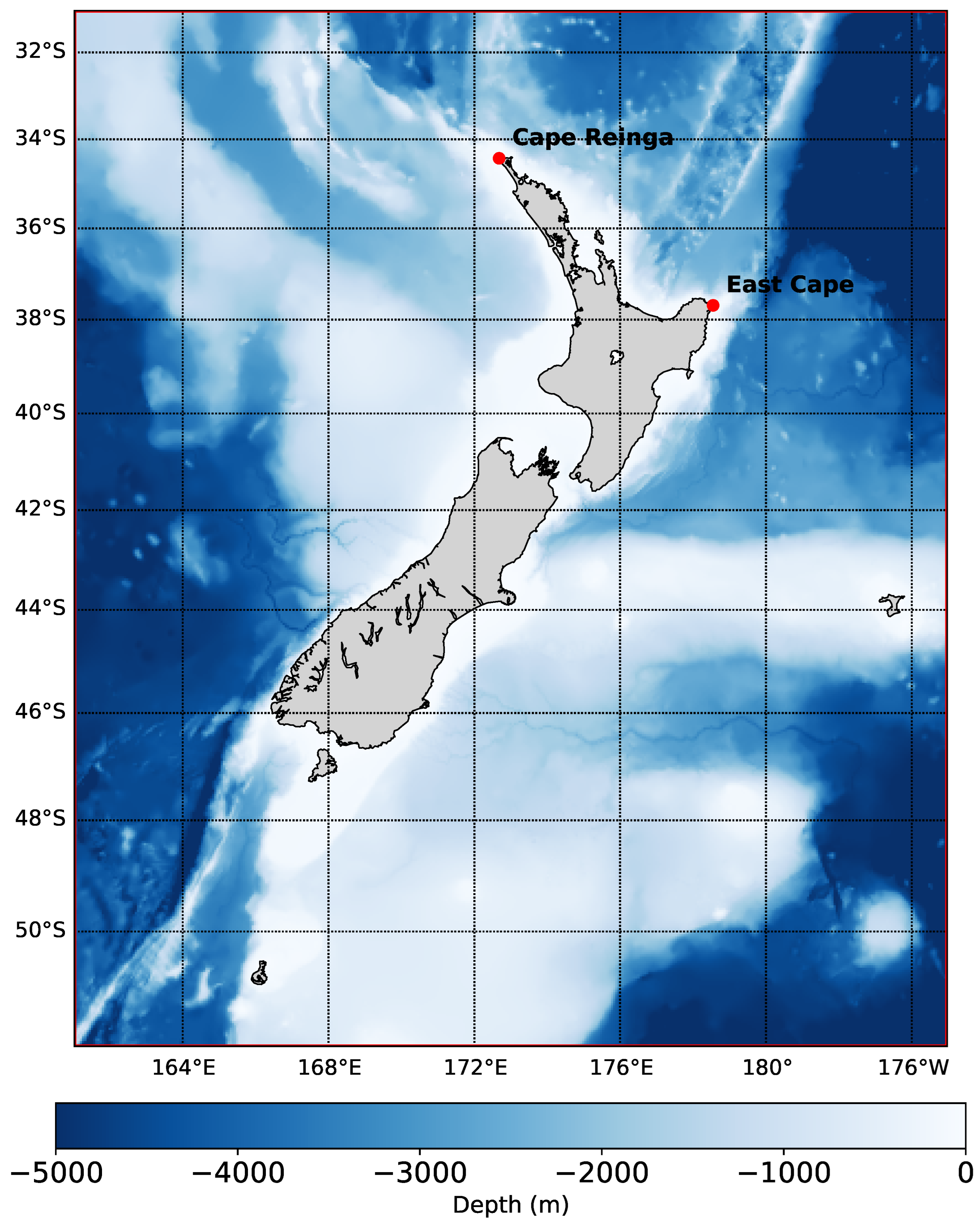
The Moana OFS ocean circulation model is implemented using the Regional Ocean Model (ROMS) version 3.9 [33] for the Aotearoa, New Zealand, domain, building on the configuration described by [34] for the 25+-year Moana hindcast, with the addition of 4D-Var assimilation of near-real-time observations. The model domain shown in Figure 1 covers an area from approximately 161 to 185 degrees East and 52 to 31 degrees South, with a resolution of about 5 km, comprising $467\times 397$ grid cells. The domain was selected to encompass most of the NZ Economic Exclusive Zone, including the Auckland and Chatham Islands, while positioning the open boundaries at a sufficient distance from New Zealand’s main islands. It also ensures that both the Tasman Front in the north and the Sub-Tropical Front in the south enter the domain through the western boundary, all while considering the computational requirements for delivering high-resolution forecasts in an operational context. The model’s bathymetry was derived from a combination of GEBCO [35] and local sources, such as navigation charts and echo sounder surveys. The model bathymetry is increasingly nudged towards that of the global model, providing boundary conditions throughout a 200 km zone, so that it is exactly equal to the outer model at the boundary.

The configuration is nested within the Mercator “Global Ocean Physics Analysis and Forecast” [36]. This product is provided by Copernicus Marine Service (CMEMS) and contains daily 3D ocean physical variables for up to 10 days in the future with 1/12-degree resolution and 50 vertical layers. We used radiation conditions for tracers at the open boundaries, coupled with a nudging zone where time-scales decrease from 1 day⁻¹ at the boundary to 0 at approximately 200 km towards the domain interior. The 3D velocities were clamped to the outer model. For the free surface and barotropic velocities, a combination of implicit Chapman and Flather boundary conditions was used, respectively. Reference [37] showed that these conditions yield optimal results for representing tides in coastal models.

Atmospheric forcing data comes from the European Centre for Medium-Range Weather Forecasts (ECMWF) atmospheric Integrated Forecast System (IFS)—the same product used for the “Global Ocean Physics Analysis and Forecast”. This dataset includes hourly 10 m winds, air temperature, relative humidity, precipitation rate, downward short- and long-wave radiation, and sea-level pressure. ROMS internally calculates upward long-wave radiation. The model incorporates climatological values for 42 New Zealand rivers’ fluxes, sourced from the www.data.govt.nzportal (accessed on 19 March 2026).

Following [38], tides were included at the open boundaries as a separate spectral forcing, with harmonics provided by the TPXO global tidal solution [39].

2.2. Data Assimilation Configuration: ROMS 4D-Var

4D-Var applies variational calculus to determine adjustments to the model’s initial and boundary conditions, as well as its forcing, in order to minimize the differences between observations and the model trajectory—within a least-squares framework—over a defined assimilation window [40]. The objective is for the model to reproduce all observations consistently in time and space, using its own physical dynamics while accounting for uncertainties in both the observations and the background state (model prior solution—before the data assimilation is performed). This process yields an ocean-state estimate, or analysis, that is dynamically balanced and fully consistent with the nonlinear model equations.

In the operational system, we used 3-day assimilation windows to generate initial conditions for 7-day forecasts. After sensitivity tests, we decided to use five inner loops and one outer loop in the 4D-Var minimization process. This allowed for a proper convergence of the 4D-Var cost function, while avoiding overfitting to the observations and keeping the computational cost affordable. Scalability tests were conducted with 2, 5, 10, 15, 20, and 35 inner cycles. Using the minimization of the 4D-Var cost function as standard for comparison and with the available computational infrastructure in mind, we concluded that 5 was the ideal number after which decreasing reductions in the cost function were achieved with an increasing number of inner cycles. Similarly, test runs indicated longer assimilation windows could benefit the solution. This is particularly true when in situ observations are scarce. In an observation-rich reality provided by the Mangōpare sensors this becomes less of a problem, emphasizing the computational cost of the simulation as the main bottleneck.

The background error covariance was obtained from a 25-year free-run integration of the simulation configuration. This hindcast dataset is described by [34].

For observation representativeness errors, we used the higher value between the instruments accuracies and the standard deviation of the observations in each grid cell and assimilation window. This approach is common for other ocean assimilation systems, such as the ones described in [11,41]. In addition, a background check filter was used to exclude any observation that deviated by a observation-type dependent number from the background value. We used two standard deviations for altimeters and in situ temperature and four for sea surface temperature. As a result, at any given cycle less than 1% and $\approx 9 \pm$ 6% of the SSH and temperature observations (respectively) were rejected. There was no clear spatial or temporal pattern in the observation rejection. The mean and standard deviation values for each type of observation assimilated are presented in

Table 1. Mean and standard deviation errors for the background and analysis, averaged in the whole domain and through the entire period of model integration presented. The last column presents the number of observations per assimilation cycle for each observation type.

Observation Type	Background	Analysis	Number Obs.
SSH	0.04 ± 0.07 m	0.005 ± 0.03 m	13,456.81 ± 5918.66
SST	0.19 ± 0.10 °C	0.05 ± 0.04 °C	143,678.01 ± 90,948.80
T profile	0.16 ± 0.17 °C	0.01 ± 0.13 °C	6751.70 ± 2335.59

.

The ROMS model configuration files for the analysis generation are available at [42].

2.3. Observing System

The observing component of the Moana OFS is an integrated framework that facilitates near-real-time observations and assessments of ocean conditions. It represents a pioneering initiative that combines advanced ocean sensing, data collection from fishing vessels, and collaborative partnerships between scientists and Māori communities. This comprehensive approach not only provides essential marine datasets but also fosters sustainable practices in the fishing industry. The observing system supports near-real-time monitoring of marine conditions, helping in the assessment of risks related to marine extremes and climate change impacts on fisheries. Therefore, this innovative system is essential for improving marine forecasts, safeguarding ocean health, and bolstering the blue economy. A full description of the observation system and its implementation is provided by [24].

For operational ocean forecast purposes, the observations assimilated comprise the Mangōpare in situ temperature profiles, sea surface temperature (SST) from the OSTIA product [43], and near-real-time Global Ocean Along Track L3 Sea Surface Heights (SSHs) from Copernicus [44] with the global mean bias in relation to the regional simulation removed and the tidal signal added. This is often necessary as the mean sea levels used to calculate anomalies in the satellite observations, in global simulations, and in regional domains differ. So, they need to be brought to the same reference before assimilation.

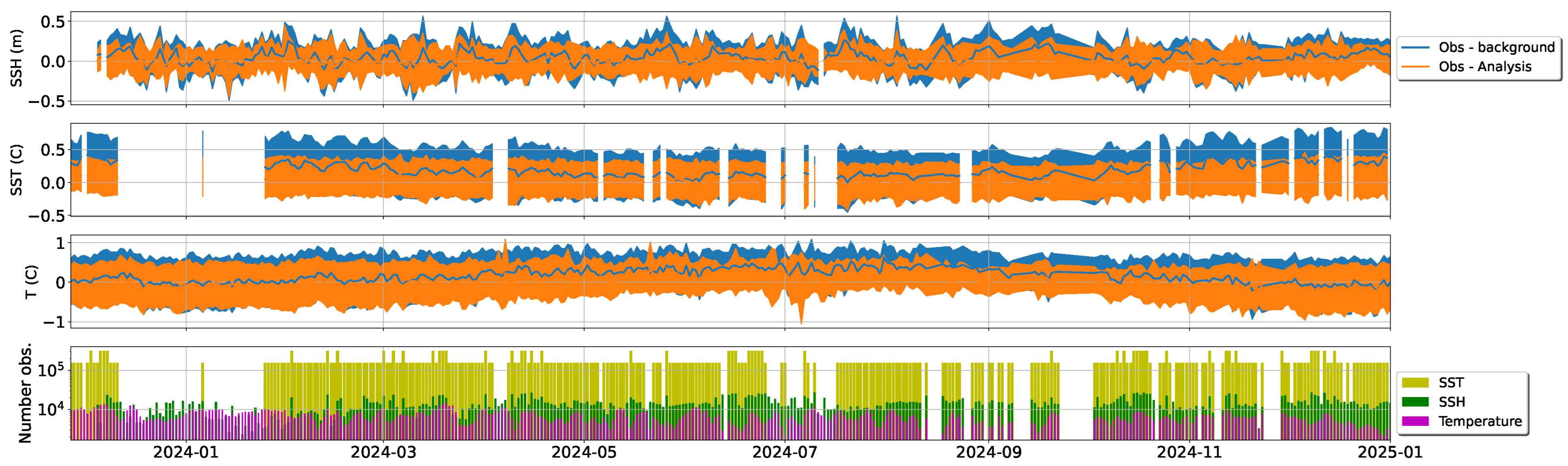
The bottom panel in Figure 2 presents the average number of observations by model grid cell per cycle. It shows the observation system provides an almost uniform coverage for SSH, while the in situ dataset that comprises all the subsurface observations is inherently scattered in both time and space due to the nature of the fishing activity. For SST, problems in the operational acquisition of the OSTIA product lead to gaps in the otherwise near uniform coverage. We purposely kept Argo profiles from the assimilation as independent observations for model evaluation.

2.4. Moana OFS Design and Architecture

The Moana OFS is designed to run daily, producing real-time 7-day forecasts of three-dimensional (3D) ocean physical conditions. The system architecture is partitioned into three distinct, sequential stages: pre-processing, model execution (run), and post-processing.

• Pre-processing: This stage handles the download, quality control, and preparation of all necessary external data. Observational and forcing data are formatted for input into the ROMS model, including any required spatial or temporal interpolation to the model grid.
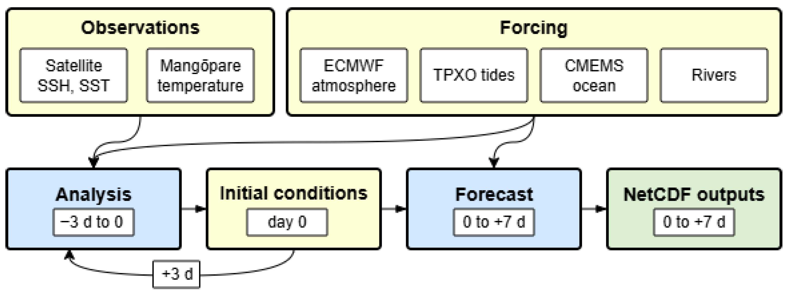
• Model execution: The analysis and forecast runs are conducted sequentially. The 4D-Var analysis is restarted from the previous analysis run three days prior, and the subsequent 7-day forecast is initialized using the resulting current analysis state.
• Post-processing: The final stage computes the model output, interpolating it to specific vertical levels. The results are generated as NetCDF files, organized into surface fields and 3D level-interpolated fields, designed to optimize data use and dissemination.

The system is deployed on a High-Performance Computing (HPC) cluster. The computational resources are allocated as follows: 121 CPU cores for the ROMS 4D-Var analysis run and 28 CPU cores for the non-linear ROMS forecast run. All tasks within the operational chain are orchestrated and managed by dedicated scheduling software. The workflow of these tasks is illustrated in the schematic diagram shown in Figure 3. Due to limitations in storage capacity and cost, the system only archives the most recent seven days of analysis and forecast output at any given time.

Gaps in the forecast time series are typically a consequence of diverse operational failures, including issues with external data download, HPC blackouts, power outages, and problems with the task orchestration software. These challenges are commonly encountered by national operational agencies and regional forecast systems.

The Moana OFS commenced operational production in October 2023 and maintained a daily execution frequency until May 2025. This study focuses on the results spanning the period from October 2023 to January 2025. This approx. 1 year of results represents 458 integrations of the data assimilation system providing enough information to access its general behavior. This is only a minimal time span for a full system evaluation, so conclusions about seasonal behavior of the data assimilation system should be made with care. That said, the results from 25-year free-running hindcast used as the base configuration for the Moana OFS did not show a seasonal bias [34]. Therefore, we do not expect it to be present in the assimilative system.

3. Evaluation of the Data Assimilation System

The time series of “observation—background” (innovation), “analysis—background” (increment), and the number of observations per provenance for each assimilation window are presented in Figure 2. Although the Mangōpare sensors in the Moana Project provide unprecedented coverage of Aotearoa’s New Zealand coastal seas, the number of in situ temperature observations is still approximately one order of magnitude smaller than those from satellite SST. Together with the relatively high number of along-track satellite SSH observations, this means the analysis of the Moana OFS is predominantly constrained at the surface.

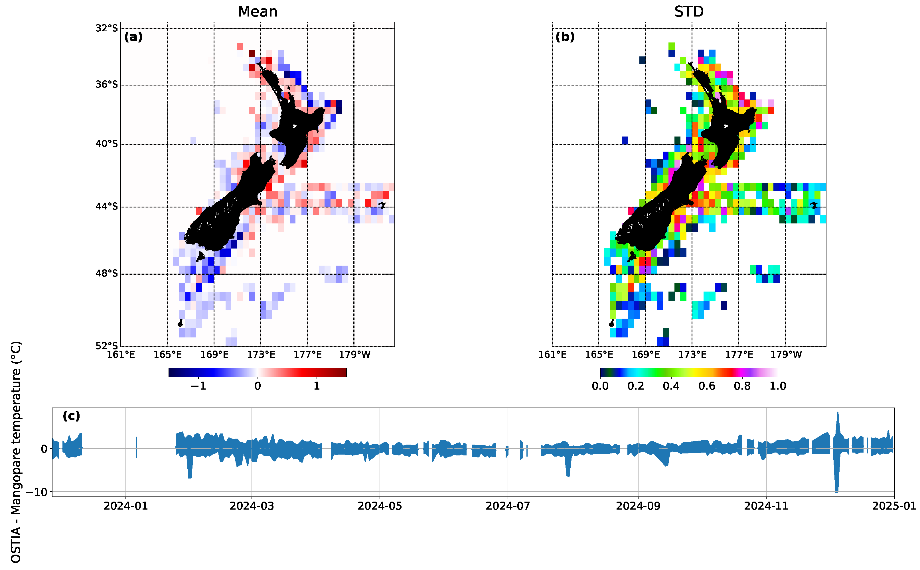
As the background at each cycle is initialized from a previous analysis, a better fit to the observations in relation to a free run is to be expected as it carries information from the previous assimilation cycles. That said, the one year of operational run indicates a seasonal behavior in the temperature bias, with the simulation having a cold SST bias in the summer and warm subsurface temperature bias in the winter. These biases were identified by [34] in the hindcast used to adjust the background configuration and calculate the error covariances used in the operational system. At the same time, we demonstrated that the OSTIA SSTs tend to be too warm during the summer in relation to in situ observations (see Figure 4c). The assimilation process with the inclusion of the relatively large number of in situ observations from the Mangōpare sensors effectively reduces both the mean bias and its spread (increments < innovations), almost eliminating it completely. The global mean and standard deviations of the errors are presented in Table 1, showing the magnitude of the reduction.

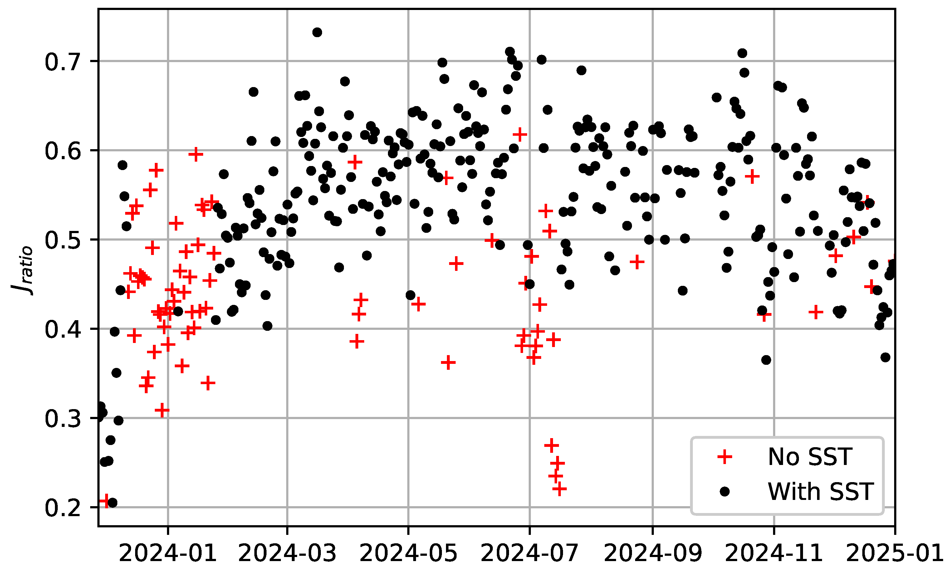
To help understand the time series presented in Figure 2, we analyze the cost function minimization ratio ($J_{ratio}=J_{final}/J_{initial}$) in Figure 5. This quantity indicates how effective the 4D-Var algorithm is in reducing the values of the initial cost function. Although the final values are consistently lower than the initial values, indicating a reduction in the cost function, there are two features that raise questions: (1) the apparent seasonal behavior in $J_{ratio}$ with stronger minimization during summer months; and (2) an important difference as a consequence of SST observations being present or not, especially for periods of time when SST is absent for a sequence of cycles. While (1) can be associated with the model SST bias discussed above, (2) requires a better understanding of the relations between the different observation types and how the unchanging system configuration behaves when the largest source of data (OSTIA SST) is absent.

Since the Mangōpare observations cover the coastal seas in a region of high cloud cover, the accuracy of the OSTIA SST product can be questioned. To help shed some light on this issue, we compared the OSTIA product with the in situ observations in the top 10 m of the water column, binned to 0.5-degree cells to follow the Ministry of Primary Industries regulations in Aotearoa, New Zealand, and protect the locations of the fishing events. The results presented on the maps in Figure 4a,b indicate that the OSTIA SSTs are consistently warmer than the in situ temperatures close to the coast, especially around the North Island. The opposite is true for deeper waters and in the Southland Current in the southeast corner of the South Island. Moreover, the time series in Figure 4c shows that the warm trend is consistent over time, with individual differences reaching ±2.5 °C at any given assimilation window—with occasional larger values reaching 10 °C. While these differences can be in part explained by temperature gradients between the surface and 10 m, the large values and consistency in time indicates the OSTIA product overestimates the temperatures in Aotearoa’s near-shore and coastal seas. The extreme values are particularly worrisome, as they show the product completely misses processes and events captured by the in situ observations. The upwelling region on the northern tip of the North Island and the eddy dynamics on the eastern extremity of the North Island are good examples of processes not represented in OSTIA. Moreover, the cold SSTs over the Southland Current in the OSTIA product can have important repercussions on the regional dynamics by inducing errors in the cross-shelf gradients.

This bias between the satellite product and the in situ observations can, at times, pull the analysis in different directions and impact the minimization of the cost function. In addition, since the system was developed and tuned with the full set of observations in mind, the eventual absence of the SST product for a sequence of cycles can degrade the solution. The differences in $J_{ratio}$ in Figure 5 indicate a possible overfitting to the remainder observations when the SST product is not available. Such overfitting is usually identified by atypical low values of the cost function and reductions in the increment and innovation for the available observations. The reduction in $J_{ratio}$ is particularly evident in the low values in July 2024 (the beginning of the time series must be viewed as an adjustment period), indicating an abrupt strong minimization in relation to Mangōpare and the satellite SSH. Corroborating the overfitting hypothesis, we notice a reduction in the innovation and increment for both SSH and in situ observations in Figure 2. This has the potential to degrade the solution, especially at the surface by perturbations generated from the assimilation of the in situ profiles. Such “overfitting” is shown in the error and $J_{ratio}$ values presented in

Table 2. Mean and standard deviation of the analysis increments for the top (depth < 20 m) and lower (depth > 20 m) portions of the assimilated temperature (°C) profiles, separated by whether the OSTIA SST product was included in the assimilation or not. We also present the ratio $J_{ratio}$ indicating the effectiveness of the assimilation system in reducing the cost function.

Metric	Analysis (with SST)	Analysis (No SST)
T (<20 m)	0.26 ± 0.11 °C	0.23 ± 0.12 °C
T (>20 m)	0.14 ± 0.08 °C	0.09 ± 0.11 °C
$J_{ratio}$	0.55 ± 0.09	0.44 ± 0.08

. When OSTIA SSTs are not available, the increments for the in situ observations and $J_{ratio}$ decrease. Although the decreases in mean increment values close to the surface are not very large, these can become important in particular cases. For example, for 14 July 2024 there are big jumps in the $J_{ratio}$ (0.24) and the mean increment for the temperature in the upper 20 m of the water column (0.17 °C).

To solve the overfitting problem a more robust observation acquisition system is necessary. Moreover, moving to L3 satellite SST observations would not only avoid problems with misrepresented process but also provide multiple information sources when different satellites are included. This can help avoid a complete blackout on this observation type and minimize any overfitting issues.

Geographical Distribution of the Analysis Increments

Figure 2 gives a general overview of the performance of the analysis in the region as a whole and its variability over time. However, in a dynamically rich region such as Aotearoa, New Zealand, local differences in model performance are to be expected. Areas of stronger variability such as the East Auckland Current, Southland Current, and the Sub-Tropical Front tend to represent particular challenges to the analysis often related to errors originated in the background solution. Similarly, larger analysis “errors” are expected where local and sub-grid scale processes are important. Good examples are the upwelling regions of Cape Reinga (north extremity of the North Island) and East Cape (east tip of the North Island) (highlighted in Figure 1) which temperature signals are sub-represented in the OSTIA SST product.

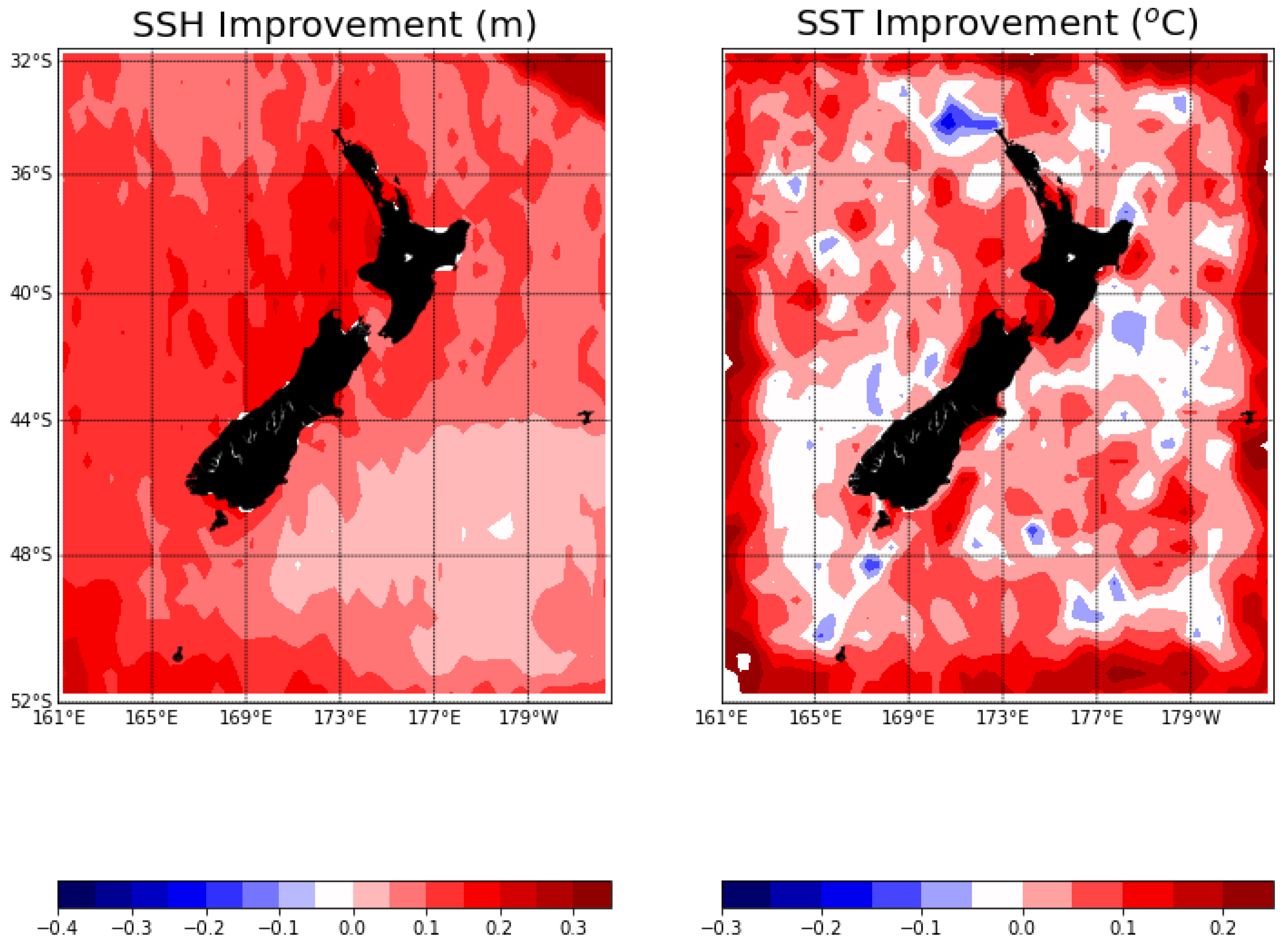
To support the evaluation of the analysis performance at the surface, Figure 6 presents maps of SSH and SST improvements, calculated as the difference between the modulus of the innovation and the modulus of the increment. Therefore, positive (negative) values represent an improvement (degradation) in the analysis relative to the background, using the observation assimilated as the reference.

The results for SSH show the analysis outperform the background through the whole domain. There are particular important improvements in the west coast of both islands, with values above 15 cm. Also, the regions of the East Auckland Current (northeast of the North Island) and the Southland Current below Dunedin show improvements in the order of 10 cm. These are the main currents influencing Aotearoa, New Zealand, and such improvements are expected to have important repercussions in the regional dynamics.

The improvements in SST are somewhat more complex. There is a clear better fit to the OSTIA product near the domain boundaries, which reflect differences between the Mercator global model used for boundary conditions and the observational product. In addition, there are improvements of the order of 0.1 °C in coastal waters around Aotearoa, New Zealand—in particular on the west coast and Cook Strait. The main regions where we see a negative comparison against OSTIA are at Cape Reinga and East Cape, where we know the observational SST product misrepresent the upwelling systems. Therefore, these negative values need to be taken carefully.

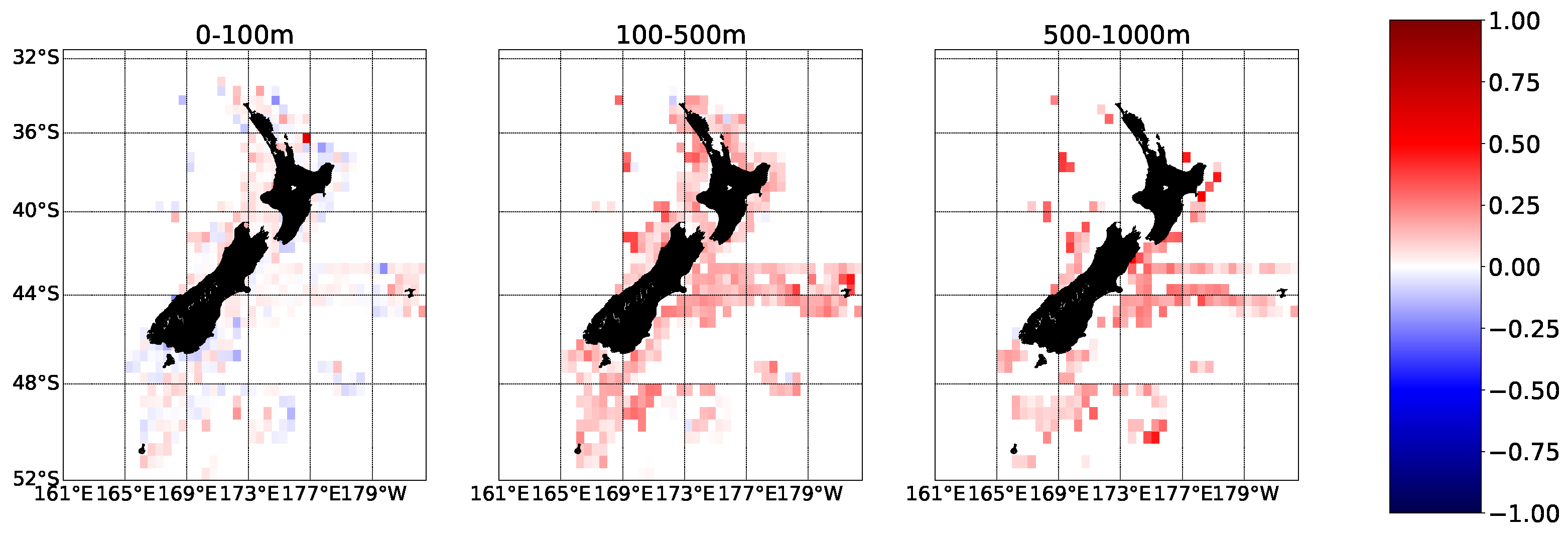
In fact, analyzing the comparison of the in situ Mangōpare observations in Figure 7 we see clear improvements in the two regions mentioned above. Moreover, the magnitude of the improvement in the top 100 m of the water column is 5 to 10 times larger than the negative values in Figure 6. This gain in performance of the analysis is prominent throughout the coastal waters around both islands and more important in the deeper layers. This can be related to a combination of the strong constraint to the surface provided by the large number of SST observations, the disagreements between the near-surface in situ observations and the OSTIA SST product presented in Figure 4, and the richer dynamics of the near-surface ocean being more challenging for the model. For deeper layers, the Mangōpare observations are the only constraint to the model solution. This conclusion on the influence of the OSTIA SST is corroborated by the results present in Table 2, as described in more detail in the previous section.

The improvement in the temperature representation in the water column has a particular impact on the model capacity to capture extreme marine heatwave events. As shown by [45], the advection of temperature in the mixed layer is the main driver of extreme upper ocean heat content events on the north and east coasts. The occurrence of extremes is favored by an overall warm upper ocean over the region, while particular coastal events are triggered by local processes. According to the same authors, on the west coast of the islands the density structure down to 1000 m is the main driver. The assimilation of Magōpare observations in Aotearoa, New Zealand, is shown to provide the necessary regional and depth coverage, while capturing local variability. It provides better initial conditions for forecasting in important aquaculture regions, such as the Bay of Plenty and the Cook Strait where noticeable improvements in the temperature structure are visible.

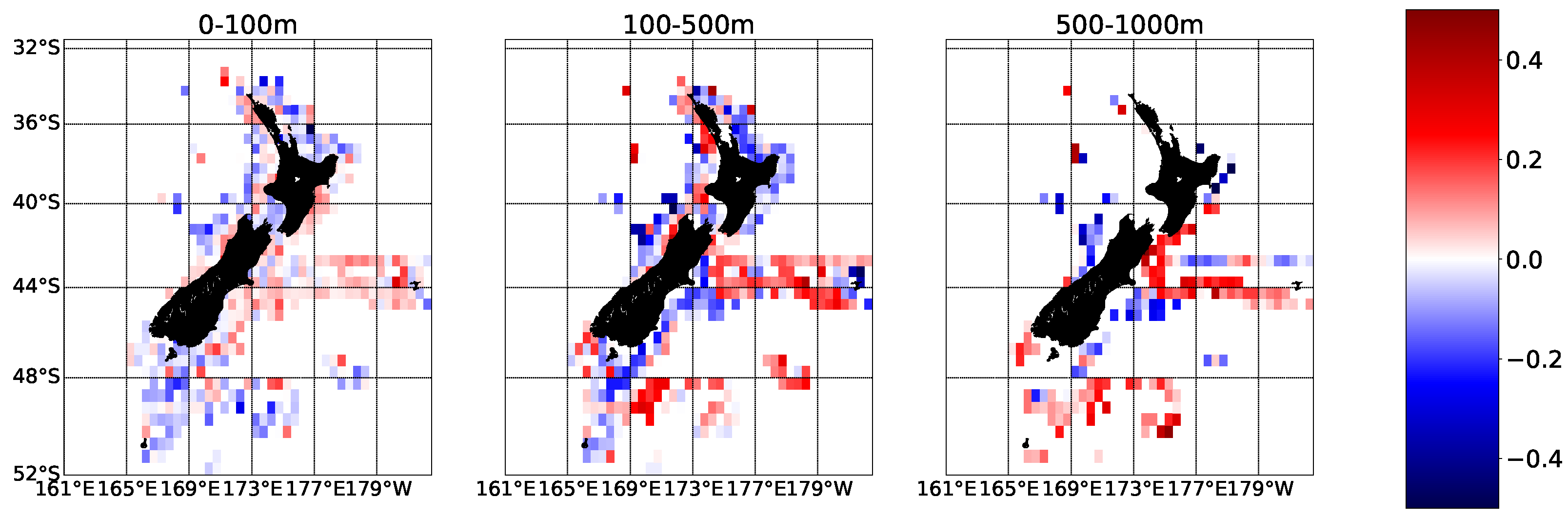
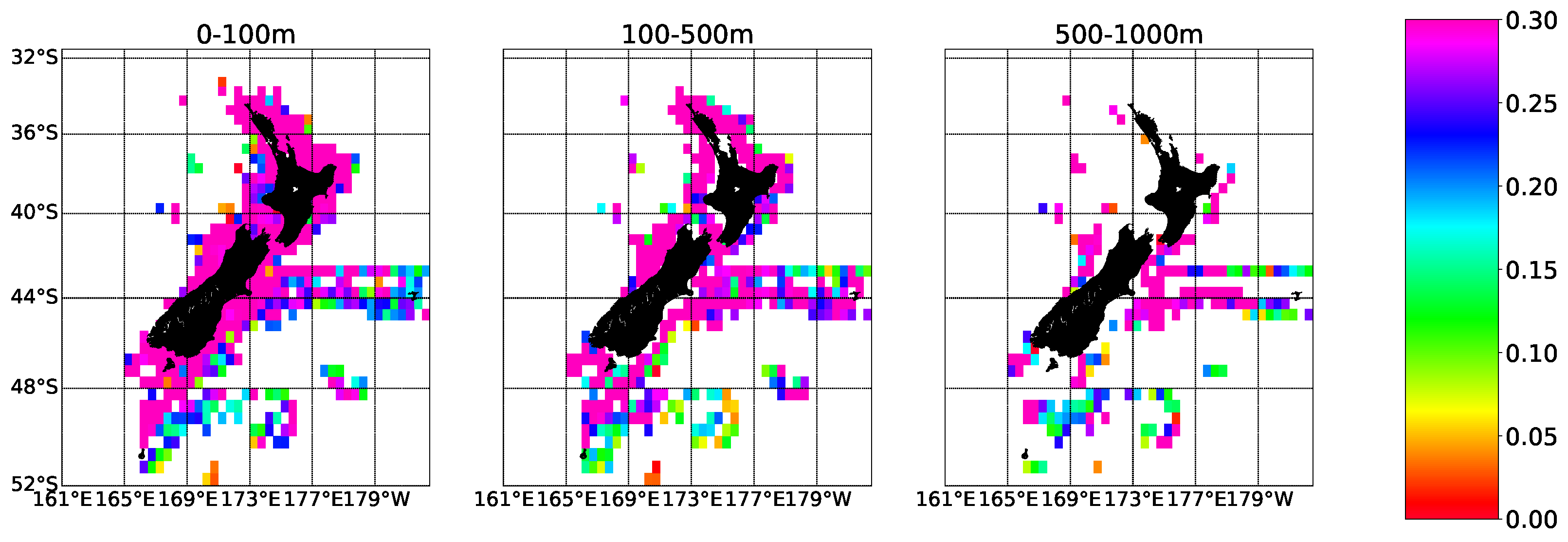
To provide a clearer understanding of the model performance in the subsurface, Figure 8 shows the analysis increments in relation to the Mangōpare in situ observations averaged in time. The analysis is ≈0.25–0.3 °C warmer than the observations in the top 100 m of the water column. This is consistent with the warm bias of the OSTIA product showed in Figure 4. Differences tend to be larger in regions of higher variability, as shown in the map of the standard deviation of the differences in Figure 9. The areas of larger standard deviations coincide with high-variability region outside Cape Reinga, the meandering East Auckland Current to the east coast of the North Island, and the energetic Southland Current.

This trend decreases in the deeper layers, although larger localized values persist in regions of high variability. Noticeably, the East Auckland Current at the East Cape in the North Island shows important mean and standard deviation differences persisting into the 100–500 m layer.

It is interesting to observe that the increments from the data assimilation in the subsurface can disturb the solution at deeper layers, where no observations—no constraints—are available. Given the longer time-scales usually associated with variability in the deep ocean, one way to minimize potential problems is to nudge the solution to climatology below a certain depth, therefore preventing any perturbations from growing. Although this was not applied in the current configuration, it should be considered for system improvement.

4. Conclusions

The unprecedented number of observations of the ocean interior and its large geographical coverage provided by the Mangōpare sensors provide a step-change improvement for the ocean operational forecast around Aotearoa, New Zealand. Most forecast systems rely on Argo profiling floats to provide information about the ocean subsurface temperature structure. Although these observations are a fundamental cornerstone of the global ocean observing system, they present significant limitations for regional applications because their coverage does not extend into waters shallower than 1000 m. The Mangōpare sensors deployed in collaboration with the fishing industry fill this coverage gap, while building strong relationships with important final users of the observations and forecasts. The result is better analyses and forecasts, as evidenced by the improvement metrics in Figure 2, Figure 6 and Figure 7.

Ref. [29] highlighted the importance of coverage over the simple number of observations in improving the model results. Although we cannot prove this is the case in the present analysis, the regional coverage provided by the Mangōpare observations is important for setting up the environment for the development and predictability of marine heatwaves, as shown by [45].

However, surface observations still constitute the bulk of the data that is assimilated in most ocean forecast systems. In the system here described, SSTs from OSTIA are present in numbers approximately an order of magnitude above any other observation type. The comparison against near-surface in situ temperature observations raises the concern that this observational product may not be accurate in the coastal seas of Aotearoa, New Zealand. Moreover, blackouts in the acquisition of the observations in time for assimilation lead to possible overfitting of the model to the in situ observations, potentially degrading the solution.

Future work on the operational system should include the substitution of the OSTIA SSTs by L3 observation sources and hardening of the data download to avoid blackouts. Having multiple SST sources would help avoid complete blackouts of this observation type. The inclusion of microwave-derived SSTs should be investigated given the frequent and large cloud coverage over Aotearoa, New Zealand. Moreover, including Argo floats and other sources of near-real-time observations, such as coastal stations and moored sensors, has the potential of increasing analysis accuracy on open waters and at the coast.

The evolution of ocean observing systems and data-assimilative operational forecasts must go hand in hand, as innovations in both fronts provide vital information to the other and help improve services that are key for ocean safety and the blue economy.