Autonomous Navigation of an Unmanned Underwater Vehicle via Safe Reinforcement Learning and Active Disturbance Rejection Control

Abstract

A two-layer control framework for unmanned underwater vehicle (UUV) navigation is proposed, combining a lower-layer active disturbance rejection controller (ADRC) with an upper-layer safe reinforcement learning (RL) policy for obstacle-avoidance navigation. The lower layer, utilizing ADRC, ensures high tracking accuracy and effective disturbance rejection, while the upper layer integrates the twin delayed deep deterministic policy gradient (TD3) algorithm, combined with a control barrier function (CBF)-based quadratic programming (QP) safety filter and safety-inspired reward shaping (SR). The method is evaluated in two simulation studies: (i) velocity and attitude control to assess tracking and disturbance rejection, and (ii) obstacle-avoidance navigation to assess learning efficiency, trajectory smoothness, and safety-related metrics. Simulation results show that ADRC achieves faster tracking and stronger disturbance rejection than a conventional proportional–integral–derivative (PID) controller. Moreover, the proposed TD3 + QP + SR scheme exhibits faster learning, smoother trajectories, and improved safety performance compared with RL baselines. These results indicate that the proposed framework enables efficient and safe UUV navigation in simulation scenarios with obstacles and disturbances.

1. Introduction

Unmanned underwater vehicles (UUVs) are widely used in ocean exploration and offshore operations. They support tasks such as scientific surveys, environmental monitoring, resource exploration, and underwater inspection and repair [1,2,3]. By working at depths and in areas that are unsafe or inaccessible for human divers, UUVs expand the scope of ocean activities. Despite these benefits, reliable UUV operation remains challenging. UUV dynamics are nonlinear and time-varying, and the motion channels are strongly coupled. Hydrodynamic parameters are also uncertain [4]. In addition, external disturbances, including currents, waves, and turbulence, can deviate the vehicle from the desired trajectory and reduce control accuracy [5]. These issues make precise navigation and control difficult, and they call for control methods that can maintain stability, tracking performance, and safety under disturbances and uncertainties.

Early UUV control studies mainly adopted classical control methods. Proportional–integral–derivative (PID) controllers and other linear designs have been widely used in UUVs because they are simple and have a long record in engineering practice [6]. However, in ocean environments, conventional controllers often show clear limitations. Accurate hydrodynamic models are difficult to obtain, and unmodeled dynamics and external disturbances can lead to large tracking errors. These issues have motivated the development of advanced and robust control approaches.

Advanced control techniques like sliding mode control (SMC), robust control, and active disturbance rejection control (ADRC) have been explored for UUVs, offering better handling of system uncertainties and disturbances [7,8,9]. In particular, ADRC has been widely studied for UUV control under uncertainties. ADRC does not need an accurate vehicle model [10]. It uses an extended state observer (ESO) to estimate total disturbance in real time. A feedback law is adopted to compensate this disturbance [11]. Compared to classical PID controllers, ADRC-based designs have demonstrated significantly improved disturbance rejection and stability for UUVs operating in waves and currents. Several studies have reported representative results. Zhang et al. designed the NTSM-ADRDC scheme for UUV 3D trajectory tracking, achieving fast error convergence and strong robustness via decoupling control and ESO-based disturbance estimation [12]. Li et al. applied a PSO-tuned ADRC to the underwater navigation of amphibious multirotor vehicles, and the resulting controller outperformed PID and SMC in response speed and disturbance rejection [13]. Zhao et al. proposed the OLOS-ADRC strategy for hybrid underwater gliders, reducing depth tracking RMSE by 83% compared to traditional ADRC and effectively resisting ocean current interference [14]. Wang et al. developed a leader–follower formation control method for multiple UUVs with ADRC as the bottom dynamic controller, enabling stable switching and maintenance between one-line and V patterns [15]. These studies exemplify the trend toward modern robust control techniques in UUVs, where disturbances are estimated and rejected in real-time to maintain performance in the face of uncertainties.

While robust lower-layer control is essential, an autonomous UUV must also make intelligent upper-layer decisions, such as avoiding obstacles and adjusting its path in real time. In the dynamic underwater environments, traditional pre-planned trajectories may be insufficient; the vehicle should react to unknown obstacles or changes in the environment as they are detected. To enable this capability in UUVs, researchers have increasingly turned to reinforcement learning (RL) methods in recent years [16,17]. Deep reinforcement learning algorithms enable a UUV to learn collision avoidance and path planning strategies via trial-and-error interactions with a simulated environment. These algorithms optimize the UUV’s behavior to achieve goals such as reaching a target, minimizing travel time and avoiding collisions. Hadi et al. proposed an adaptive path planning method based on deep RL [18]. It guided a UUV to a target in unknown environments, avoided randomly distributed obstacles and counteracted ocean current disturbances. Similarly, other studies have successfully applied RL to UUV navigation. Zhang et al. proposed an actor–critic RL controller for underactuated UUVs [19]. It simultaneously addresses 3D path tracking and obstacle avoidance, adopting a DDPG-based approach enhanced by fuzzy logic. These works show the value of reinforcement learning. An RL-based controller can learn an effective policy, rather than depending only on a fixed analytical model.

However, applying standard reinforcement learning to safety-critical systems such as UUVs operating near obstacles faces a fundamental challenge: safety cannot be guaranteed during either training or deployment. Exploration is necessary for policy improvement, but unconstrained exploration may lead to collisions or aggressive maneuvers, which is unacceptable for real underwater missions. This limitation has motivated safe RL [20,21,22,23], which explicitly incorporates safety constraints into policy learning and execution. Representative safe RL methods can be grouped into two categories.

First, constrained RL methods treat safety as an auxiliary cost and enforce a constraint budget through Lagrangian relaxation and primal–dual updates, such as constrained policy optimization and Lagrangian-based deep RL variants [24,25]. These approaches are model-free and easy to integrate, but their safety–performance trade-off can be sensitive to multiplier tuning and they may still exhibit constraint violations during exploration.

Second, shielded RL introduces an online safety layer that minimally modifies the nominal action to satisfy constraints, including action-correction safety layers, control barrier function (CBF)-based quadratic programs (QP), and predictive safety filters [26,27]. This line can provide stronger real-time constraint enforcement when the online optimization remains feasible, but it typically requires a tractable safety model and can be affected by model mismatch in complex dynamics.

In underwater navigation, these issues are amplified by strong hydrodynamic un-certainty and external disturbances. To address this gap, a two-layer control framework is developed for the UUV obstacle-avoidance navigation. The framework combines active disturbance rejection control and reinforcement learning. The main contributions are summarized as follows.

(1) A novel safety-inspired reward shaping scheme is developed, in which obstacle proximity and safety margins are explicitly encoded to provide dense guidance for safe exploration. Simulation results demonstrate that this reward design improves learning efficiency and yields faster convergence compared with ablations without safety-inspired rewards.

(2) A disturbance-rejection safe navigation architecture is formulated by coupling an upper-layer CBF-QP safety filter with a lower-layer ADRC robust tracking controller. The ADRC layer rejects model uncertainties and external disturbances, thereby reducing their impact on the safety-filtering stage and enabling the QP module to output reliable safe commands. Compared with typical shielded RL that relies mainly on a policy plus a safety layer, the proposed hierarchy explicitly incorporates a robust execution layer tailored to underwater disturbances, improving reliability under uncertainty.

(3) Extensive simulations and ablation studies are conducted under identical environment settings and the same lower-layer controller, and improved navigation performance and safety-oriented behavior are demonstrated.

2. Dynamic Model of the Unmanned Underwater Vehicle

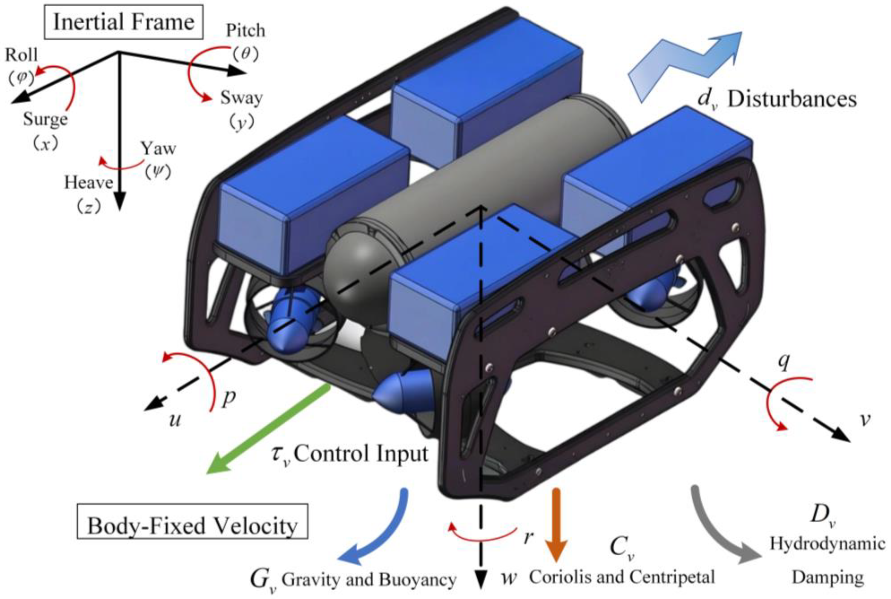
In this section, the kinematic and dynamic models of the underwater vehicle are summarized, and they are used throughout this work. An inertial frame {I} and a body-fixed frame {B} are defined as in Figure 1, and the vehicle is modeled as a rigid body moving in a fluid environment.

2.1. Vehicle Kinematics

Let the vehicle pose in the inertial frame and body-fixed velocity be denoted by $\eta$ and $v$, respectively. They are defined as:

$$\eta =\left[\begin{array}{c}{\eta }_1\\ {\eta }_2\end{array}\right]={\left[\begin{array}{cccccc}x& y& z& \phi & \theta & \psi \end{array}\right]}^{\mathrm{T}},$$

(1)

$$v=\left[\begin{array}{c}{v}_1\\ v_2\end{array}\right]={\left[\begin{array}{cccccc}u& v& w& p& q& r\end{array}\right]}^{\mathrm{T}},$$

(2)

where ${\eta }_1={\left[\begin{array}{ccc}x& y& z\end{array}\right]}^{\mathrm{T}}$ is the position vector, ${\eta }_2={\left[\begin{array}{ccc}\phi & \theta & \psi \end{array}\right]}^{\mathrm{T}}$ is the roll–pitch–yaw vector, $v_1={\left[\begin{array}{ccc}u& v& w\end{array}\right]}^{\mathrm{T}}$ is the linear velocity, and $v_2={\left[\begin{array}{ccc}p& q& r\end{array}\right]}^{\mathrm{T}}$ is the angular velocity.

The kinematic relationship between $\eta$ and $v$ is:

$$\dot{\eta }=J_v({\eta }_2)v,$$

(3)

where $J_v({\eta }_2)\in {\mathbf{R}}^{6\times 6}$ is the vehicle Jacobian mapping body-fixed velocities to inertial pose velocities.

2.2. Vehicle Dynamics

Considering the inertia, Coriolis/centripetal effects, hydrodynamic damping, and restoring forces, the vehicle dynamics can be written in the standard 6-DOF form [6]:

$$M_v\left(\eta \right)\dot{v}+C_v(v)v+D_v(v)v+G_v(\eta )={\tau }_v+d_v,$$

(4)

where $M_v\left(\eta \right)\in {\mathbf{R}}^{6\times 6}$ is the generalized inertia matrix, including rigid-body inertia and added mass, $C_v(v)\in {\mathbf{R}}^{6\times 6}$ is the Coriolis and centripetal matrix, $D_v(v)\in {\mathbf{R}}^{6\times 6}$ represents hydrodynamic damping, $G_v(\eta )\in {\mathbf{R}}^{6\times 1}$ collects restoring forces and moments induced by gravity and buoyancy, ${\tau }_v\in {\mathbf{R}}^{6\times 1}$ is the control input vector, and $d_v\in {\mathbf{R}}^{6\times 1}$ denotes ocean current disturbances and model uncertainties.

2.3. Control Objective

The objective of this work is to design a control system that enables the UUV to autonomously navigate to a predefined target position while safely avoiding obstacle regions in the workspace. Based on the 6-DOF vehicle kinematic and dynamic models introduced above, the control input ${\tau }_v$ is required to drive the vehicle position $p={\left[\begin{array}{ccc}x& y& z\end{array}\right]}^{\mathrm{T}}$ to a neighborhood of a desired target $p_d={\left[\begin{array}{ccc}{x}_d& y_d& z_d\end{array}\right]}^{\mathrm{T}}$ and simultaneously regulate the vehicle velocity to zero, ensuring smooth and stable convergence.

During the navigation process, the vehicle must satisfy safety constraints imposed by environmental obstacles, such that collision-free motion is guaranteed for all time. Moreover, the controller should explicitly account for speed limitations and be robust against modeling uncertainties and external disturbances, including hydrodynamic parameter variations and ocean currents.

3. Hierarchical Control Framework

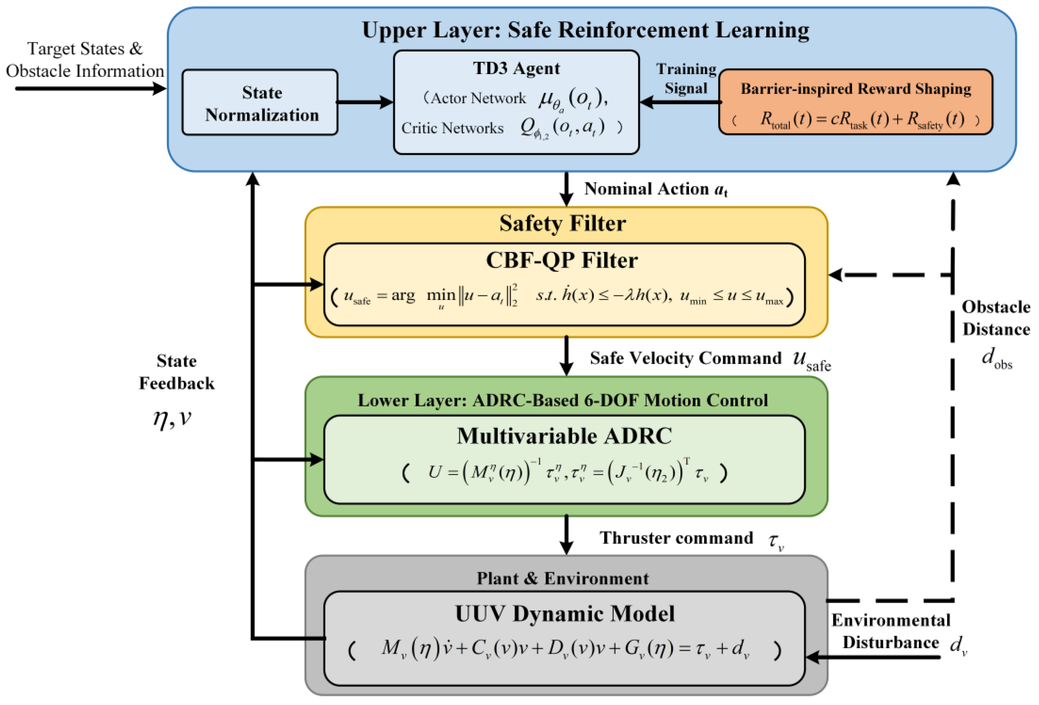
As shown in Figure 2, a two-layer control framework is proposed. The upper layer realizes safe deep reinforcement learning: a TD3 agent generates nominal velocity commands using a safety-inspired reward, and a CBF–QP module filters these actions to satisfy safety constraints. The lower layer adopts a multivariable ADRC design, including velocity and attitude controllers, to robustly track the filtered commands under uncertainties and disturbances.

3.1. Lower Layer: ADRC-Based 6-DOF Motion Control

In Figure 2, the upper-layer safe reinforcement learning controller generates commanded velocity references for the lower-layer ADRC system. Accordingly, the lower-layer controller consists of two components: an attitude controller responsible for stabilizing the UUV orientation, and a velocity controller responsible for tracking the commanded velocities along the x-, y-, and z-axes.

3.1.1. Design of the Attitude Controller

According to the kinematic relationship (3), the dynamic model (4) can be rewritten as:

$$M_v^{\eta }(\eta )\ddot{\eta }+C_v^{\eta }(\eta ,\dot{\eta })\dot{\eta }+D_v^{\eta }(\eta ,\dot{\eta })\dot{\eta }+G_v^{\eta }(\eta )={\tau }_v^{\eta }+d_v^{\eta }\eta ,$$

(5)

where $M_v^{\eta }={\left({J_v}^{-1}({\eta }_2)\right)}^{\mathrm{T}}{M}_v(\eta ){J_v}^{-1}({\eta }_2)$, $C_v^{\eta }={\left({J_v}^{-1}({\eta }_2)\right)}^{\mathrm{T}}\left(C_v(v)-M_v(\eta ){J_v}^{-1}({\eta }_2){\dot{J}}_v({\eta }_2)\right){J_v}^{-1}({\eta }_2)$, $D_v^{\eta }={\left({J_v}^{-1}({\eta }_2)\right)}^{\mathrm{T}}{D}_v(v){J_v}^{-1}({\eta }_2)$, $G_v^{\eta }={\left({J_v}^{-1}({\eta }_2)\right)}^{\mathrm{T}}{G}_v(\eta )$, ${\tau }_v^{\eta }={\left({J_v}^{-1}({\eta }_2)\right)}^{\mathrm{T}}{\tau }_v$, and $d_v^{\eta }={\left({J_v}^{-1}({\eta }_2)\right)}^{\mathrm{T}}{d}_v$.

Simplify the dynamic model (5) to the following form:

$$\ddot{\eta }=U+f,$$

(6)

where $f={\left(M_v^{\eta }(\eta )\right)}^{-1}\left(-C_v^{\eta }(\eta ,\dot{\eta })\dot{\eta }-D_v^{\eta }(\eta ,\dot{\eta })\dot{\eta }-G_v^{\eta }(\eta )+d_v^{\eta }\eta \right)$ and $U={\left(M_v^{\eta }(\eta )\right)}^{-1}{\tau }_v^{\eta }$. $U={\left[\begin{array}{cccccc}{u}_1& u_2& u_3& u_4& u_5& u_6\end{array}\right]}^{\mathrm{T}}$ is a virtual control vector, where the components ${\left[\begin{array}{ccc}{u}_1& u_2& u_3\end{array}\right]}^{\mathrm{T}}$ denote the control quantities for the position loop ${\eta }_1$, and the components ${\left[\begin{array}{ccc}{u}_4& u_5& u_6\end{array}\right]}^{\mathrm{T}}$ denote those for the attitude loop ${\eta }_2$.

The term $f$ in the simplified model (6) is regarded as the total disturbance, for which the ESO is adopted to implement estimation and compensation. Therefore, the attitude control loop can be decoupled into three single-input single-output (SISO) systems to enable independent controller design. The ESO corresponding to the attitude loop can be formulated as follows:

$$\left\{\begin{array}{l}{\dot{z}}_{1i}=z_{2i}+l_{1i}\left(x_{1i}-z_{1i}\right)\\ {\dot{z}}_{2i}=z_{3i}+l_{2i}\left(x_{1i}-z_{1i}\right)+u_i\\ {\dot{z}}_{3i}=l_{3i}\left(x_{1i}-z_{1i}\right)\end{array}\right.,$$

(7)

where $i=4,5,6$. The vector ${\left[\begin{array}{ccc}{z}_{14}& z_{24}& z_{34}\end{array}\right]}^{\mathrm{T}}$ denotes the observed values of the attitude, attitude derivative and total disturbance for the $\phi$ loop, respectively; ${\left[\begin{array}{ccc}{z}_{15}& z_{25}& z_{35}\end{array}\right]}^{\mathrm{T}}$ denotes those for the $\theta$ loop, respectively; and ${\left[\begin{array}{ccc}{z}_{16}& z_{26}& z_{36}\end{array}\right]}^{\mathrm{T}}$ denotes those for the $\psi$ loop, respectively. $l_{1i}$, $l_{2i}$, and $l_{3i}$ denote the observation gains of the ESO, respectively. The vector ${\left[\begin{array}{ccc}{x}_{14}& x_{15}& x_{16}\end{array}\right]}^{\mathrm{T}}$ denotes the measured value of ${\eta }_2$.

The virtual control input $u_i$ of the $i$-th loop can be obtained by solving the following equation:

$$u_i=k_{1i}\left(x_{id}-z_{1i}\right)+k_{2i}\left({\dot{x}}_{id}-z_{2i}\right)-z_{3i}+{\ddot{x}}_{id},$$

(8)

where $i=4,5,6$. $x_{4d}$, $x_{5d}$, and $x_{6d}$ denote the reference signals for the $\phi$, $\theta$, and $\psi$ loops. $k_{1i}$ and $k_{2i}$ are the parameters of the feedback controller (8).

3.1.2. Design of the Velocity Controller

The velocity controller is designed to track the command signal generated by the upper-layer module. According to Equation (6), the velocity dynamics can be written in the following form:

$${\dot{v}}_I=U+f,$$

(9)

where $v_I=\dot{\eta }={\left[\begin{array}{cccccc}{v}_x& v_y& v_z& v_{\phi }& v_{\theta }& v_{\psi }\end{array}\right]}^{\mathrm{T}}$ denotes the velocity vector in the inertial frame, $v_I=J_v({\eta }_2)v$.

The ESO corresponding to the velocity loop can be formulated as follows:

$$\left\{\begin{array}{l}{\dot{z}}_{1i}=z_{2i}+l_{1i}\left(x_{1i}-z_{1i}\right)+u_i\\ {\dot{z}}_{2i}=l_{2i}\left(x_{1i}-z_{1i}\right)\end{array}\right.,$$

(10)

where $i=1,2,3$. $z_{11}$ and $z_{21}$ denote the observed values of the velocity and total disturbance for the $v_x$ loop, $z_{12}$ and $z_{22}$ denote the observed values of the velocity and total disturbance for the $v_y$ loop, $z_{13}$ and $z_{23}$ denote the observed values of the velocity and total disturbance for the $v_z$ loop.

The virtual control input $u_i$ of the $i$-th loop can be obtained by solving the following equation:

$$u_i=k_{1i}\left(x_{id}-z_{1i}\right)-z_{2i}+{\dot{x}}_{id},$$

(11)

where $i=1,2,3$. $x_{1d}$, $x_{2d}$, and $x_{3d}$ denote the command signal for the $v_x$, $v_y$, and $v_z$ loops. $k_{1i}$ is the parameter of the feedback controller (11).

3.2. Upper Layer: Safe Reinforcement Learning for Goal-Directed Navigation

The upper layer serves as a decision-making module that generates high-layer command signals for goal-directed navigation in cluttered underwater environments. A TD3-based policy is trained to produce efficient goal-seeking behavior under uncertainty. Safety is improved through barrier-inspired reward shaping and a CBF-based QP safety filter.

3.2.1. Reinforcement Learning Controller

The design procedure of the RL controller can be decomposed into the following key steps.

(1)

State and action definition

The upper-layer controller is formulated as a continuous-state, continuous-action reinforcement learning problem in which a policy is trained to generate nominal navigation commands for goal reaching under environmental constraints.

At time $t$, the observation vector $o_t$ consists of the position tracking error, its integral term, the measured UUV velocity, the distance to the obstacle, and the difference between the input and output of the QP-based safety filter. The action is defined as a bounded continuous vector $a_t$. It represents the upper-layer command to the lower-layer controller. Action bounds are enforced by the actor output scaling in the policy network.

(2)

Policy learning algorithm

A TD3 agent is employed due to its improved stability in continuous control. Two critic networks $Q_{{\varphi }_1}\left(o,a\right)$ and $Q_{{\varphi }_2}\left(o,a\right)$ are used to mitigate Q-value overestimation. Target policy smoothing is applied as:

$${\tilde{a}}_{t+1}=\mathrm{clip}\left({\mu }_{{\overline{\theta }}_a}(o_{t+1})+{\epsilon }_{t+1},a_{\min },a_{\max }\right),$$

(12)

$${\epsilon }_{t+1}\sim \mathrm{clip}\left(\mathcal{N}(0,{\sigma }^{2}I),-c,c\right),$$

(13)

where ${\mu }_{{\overline{\theta }}_a}$ is the target actor, ${\overline{\theta }}_a$ denotes the parameter of the target actor, $\left[a_{\min },a_{\max }\right]$ are the action bounds, $\sigma$ is the smoothing-noise standard deviation, and $c$ is the clipping level. The TD target is computed by clipped double-Q:

$$y_t=r_t+\gamma \underset{i\in \left\{1,2\right\}}{\min }{Q}_{{\overline{\varphi }}_i}\left(o_{t+1},{\tilde{a}}_{t+1}\right),$$

(14)

where $y_t$ denotes the one-step bootstrapped TD target used to train the critic, $r_t$ is the immediate reward returned by the environment, $Q_{{\overline{\varphi }}_i}$ are target critics, ${\overline{\varphi }}_i$ denote the parameters of the target critics. Each critic is updated by minimizing:

$$\mathcal{L}({\varphi }_i)={\mathbb{E}}_{\left(o_t,a_t,r_t,a_{t+1}\right)\in \mathcal{B}}\left[{\left(Q_{{\varphi }_i}(o_t,a_t)-y_t\right)}^2\right],$$

(15)

with $\mathcal{B}$ denoting a mini-batch of transitions sampled from the replay buffer. The actor is updated less frequently by maximizing:

$$\underset{{\theta }_a}{\max }{E}_{o_t\in \mathcal{B}}\left[Q_{{\varphi }_1}\left(o_t,{\mu }_{{\theta }_a}(o_t)\right)\right],$$

(16)

Target networks are updated by Polyak averaging:

$$\left\{\begin{array}{l}{\overline{\theta }}_a\leftarrow \tau {\theta }_a+(1-\tau ){\overline{\theta }}_a\\ {\overline{\varphi }}_i\leftarrow \tau {\varphi }_i+(1-\tau ){\overline{\varphi }}_i\end{array}\right.,$$

(17)

where $\tau \in \left(0,1\right)$ is the target update rate. During data collection, exploration noise ${\eta }_t$ is added to ${\mu }_{{\theta }_a}(o_t)$, and the executed action is clipped to $\left[a_{\min },a_{\max }\right]$.

(3)

Network architecture

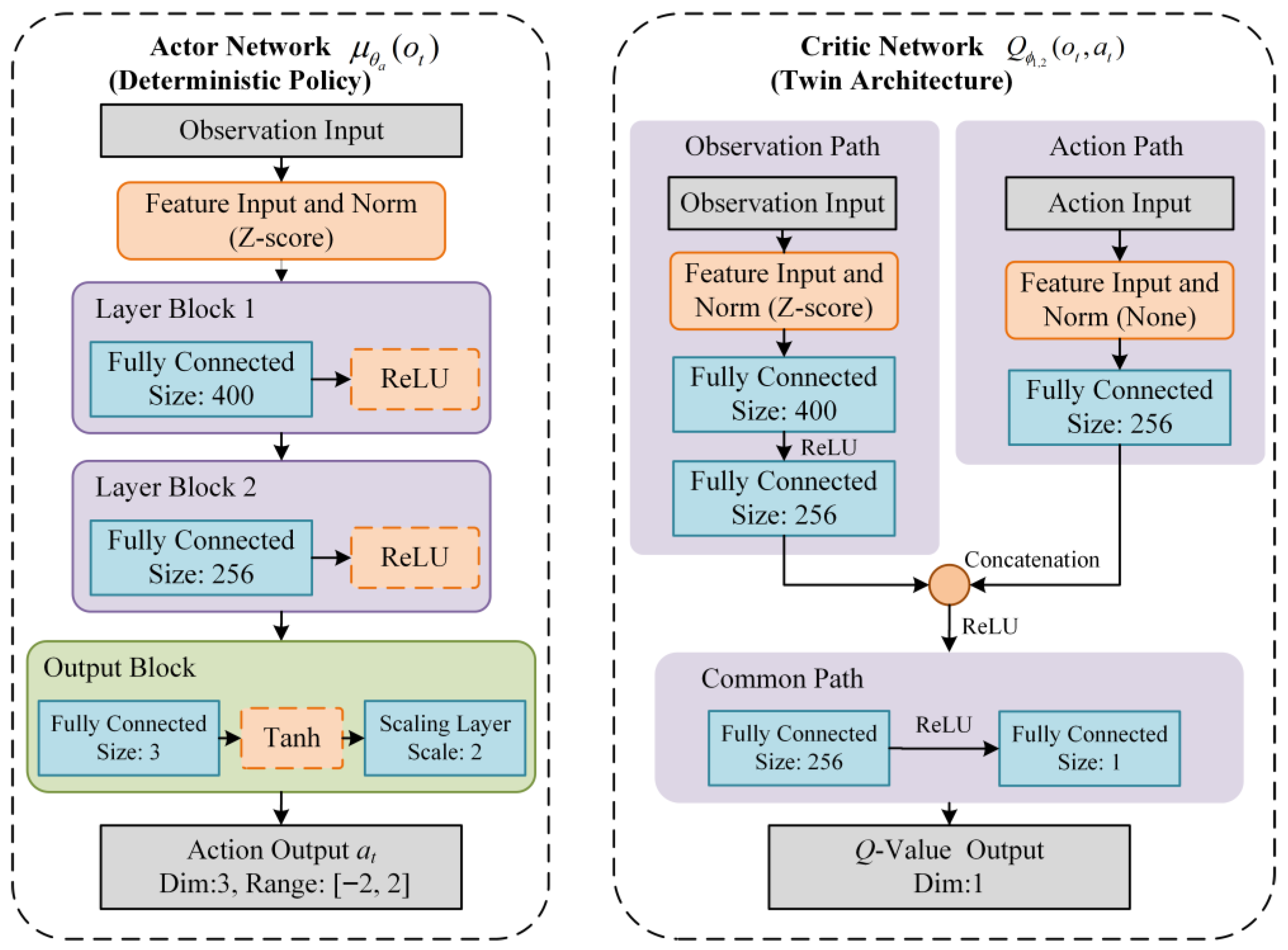
As illustrated in Figure 3, a TD3 agent is implemented with one deterministic actor and two independent critics. The actor is constructed as a feedforward network composed of an input feature layer with z-score normalization, two fully connected hidden layers with ReLU activations, and a 3-unit output layer. A tanh (⋅) nonlinearity is applied at the output, and a scaling layer is used to enforce bounded commands consistent with the action limits. Each critic adopts a dual-path architecture. The observation path used z-score normalization followed by two fully connected layers with ReLU activation, while the action path mapped the action through a fully connected layer of 256 neurons. The two feature streams are concatenated and processed by a common head to produce a scalar Q-value estimate. Two critics with identical topology but different parameters are employed to mitigate overestimation bias in value learning.

(4)

Reward shaping with task and safety terms

The learning process is guided by a composite reward:

$$R_{\mathrm{total}}(t)=c{R}_{\mathrm{task}}(t)+R_{\mathrm{safety}}(t),$$

(18)

where $c$ weights task performance relative to safety.

The task reward $R_{\mathrm{task}}(t)$ is designed in a mode-dependent form based on the Euclidean distance to the goal. An approaching mode is activated when the vehicle is far from the target to encourage rapid convergence. The formulation for the approaching mode is expressed as:

$$R_{\mathrm{task}}(t)=-c_1{d}_{\mathrm{target}}^2(t)+c_2\Delta d_{\mathrm{target}}(t),\hspace{1em}{d}_{\mathrm{target}}(t)>d_1,$$

(19)

where $d_{\mathrm{target}}$ represents the Euclidean distance between the centroid of the UUV and the target position point. The condition $d_{\mathrm{target}}(t)>d_1$ corresponds to the system being in the approaching mode. $\Delta d_{\mathrm{target}}(t)\triangleq d_{\mathrm{target}}(t-1)-d_{\mathrm{target}}(t)$, $c_1$ and $c_2$ are positive gain parameters.

A hovering mode ($d_{\mathrm{target}}(t)\le d_1$) is activated inside the target region to emphasize high-precision station keeping. The reward is designed with a selective structure as:

$$R_{\mathrm{task}}(t)=\left\{\begin{array}{l}{k}_1{e}^{-0.5\cdot d_{\mathrm{target}}^2(t)}-k_2\cdot {‖v_p(t)‖}^2-k_3\cdot {‖a(t)‖}^2+c,\hspace{1em}{d}_2<d_{\mathrm{target}}(t)\le d_1\\ k_4{e}^{-0.5\cdot d_{\mathrm{target}}^2(t)}-k_5\cdot {‖v_p(t)‖}^2-k_6\cdot {‖a(t)‖}^2+c,\hspace{1em}{d}_{\mathrm{target}}(t)\le d_2\end{array}\right.,$$

(20)

where $v_p(t)={\left[\begin{array}{ccc}{v}_x(t)& v_y(t)& v_z(t)\end{array}\right]}^{\mathrm{T}}$ is the measured velocity, $k_1$ to $k_6$ denote positive gain coefficients, and $c$ provides a constant bonus for remaining within the target region. $d_2$ is a distance threshold smaller than $d_1$, which is used to ensure the accuracy of the system’s final arrival at the target position.

Safety is enforced by a multi-zone soft penalty around each obstacle. For an obstacle center $p_{\mathrm{obs}}$, let $d_{\mathrm{obs}}(t)={‖{\eta }_1(t)-p_{\mathrm{obs}}‖}_2$. With warning and collision radii $d_{\mathrm{warning}}$ and $d_{\mathrm{collision}}$, the reward $R_{\mathrm{safety}}(t)$ is designed based on the inverse-distance and barrier-shaped mechanisms, and its formulation is given as follows:

$$R_{\mathrm{safety}}(t)=\left\{\begin{array}{l}0, d_{\mathrm{obs}}>d_{\mathrm{warning}}\\ -P_{\mathrm{base}}\cdot {\left({\displaystyle \frac{d_{\mathrm{warning}}-d_{\mathrm{obs}}}{d_{\mathrm{warning}}-d_{\mathrm{collision}}}}\right)}^2, d_{\mathrm{collision}}<d_{\mathrm{obs}}\le d_{\mathrm{warning}}\\ -\min \left(P_{\mathrm{base}}-w_{\log }\cdot \ln \left({\displaystyle \frac{d_{\mathrm{collision}}-d_{\mathrm{obs}}}{d_{\mathrm{warning}}-d_{\mathrm{collision}}}}\right),\hspace{0.33em}{P}_{\max }\right), d_{\mathrm{obs}}\le d_{\mathrm{collision}}\end{array}\right.,$$

(21)

where $P_{\mathrm{base}}$ and $w_{\log }$ tune the warning/collision severity and $P_{\max }$ saturates the penalty magnitude to prevent instability during training. Episodes are terminated upon collision, boundary violations, seabed contact, or excessive deviation from the target.

3.2.2. QP-Based Safety Filter with Control Barrier Functions

The TD3 policy outputs a nominal command $a_t$. This command can violate safety near obstacles. A QP-based safety filter is therefore added. It modifies the command only when needed. The filtered command is denoted by $u_{\mathrm{safe}}$. It is then sent to the lower-layer controller.

A control-affine model is used to describe the closed-loop motion at the decision layer,

$$\dot{x}=f(x)+g(x)u,$$

(22)

where $x$ is the system state and $u$ is the control input.

A safe set is defined by a barrier function $h(x)$ as:

$$\mathcal{C}=\left\{x\left|h(x)\le 0\right.\right\},$$

(23)

If the state starts in $\mathcal{C}$, it should stay in $\mathcal{C}$. This property is called forward invariance. Let $L_{f}h(x)={\displaystyle \frac{\mathit{\partial }h}{\mathit{\partial }x}}f(x)$ and $L_{g}h(x)={\displaystyle \frac{\mathit{\partial }h}{\mathit{\partial }x}}g(x)$ be Lie derivatives. A sufficient condition for safety is:

$$L_{f}h(x)+L_{g}h(x)u\le -\alpha \left(h(x)\right),$$

(24)

where $\alpha \left(·\right)$ is an extended class ${\mathcal{K}}_{\infty }$ function, often $\alpha (h)=\lambda h$, $\lambda >0$.

To enforce this condition online, a quadratic program is solved at each time step. It acts as a supervisory controller that enforces safety and input limits through a QP. A standard form is designed as:

$$\begin{array}{l}{u}_{\mathrm{safe}}=\arg \underset{u}{\min }{‖u-a_t‖}_2^2\\ s.t. \dot{h}(x)\le -\lambda h(x)\\ u_{\min }\le u\le u_{\max }\end{array},$$

(25)

where $a_t$ is the velocity command signal calculated by the reinforcement learning controller.

A distance-based barrier can be built as:

$$h(x)=c+d_{\mathrm{warning}}^2-d_{\mathrm{obs}}^2-k{\dot{d}}_{\mathrm{obs}},$$

(26)

where $c\ge 0$ and $k>0$ are design constants. Its derivative can be written as:

$$\dot{h}(x)=-2d_{\mathrm{obs}}{\dot{d}}_{\mathrm{obs}}-k{\ddot{d}}_{\mathrm{obs}},$$

(27)

By solving the constrained QP problem described in Equation (25), a safe velocity command $u_{\mathrm{safe}}$ that prevents the system from entering the warning region can be obtained, and this command is as close as possible to the velocity command signal $a_t$.

3.3. Stability and Safety Discussion

The proposed framework separates the navigation task into an upper layer and a lower layer. The lower layer uses a multivariable ADRC structure to stabilize the 6-DOF motion, and robustly tracks the velocity and attitude references from the upper layer. Its core idea is to combine hydrodynamic uncertainty, channel coupling and external disturbances into a total disturbance, which is estimated online by the ESO. The feedback control law then actively compensates for these disturbances.

For bounded disturbances, Reference [28] proves the convergence of the ESO: the observer’s estimation error is bounded, and the upper bound of this error decreases monotonically as the observer bandwidth increases. Reference [29] analyzes the closed-loop stability and shows that the system is exponentially stable when the initial observer error is sufficiently small. Thus, the lower layer provides reliable command-to-motion performance, ensuring more consistent closed-loop responses for the upper decision layer.

In the upper layer, the TD3 policy generates a bounded nominal 3D velocity command for goal-directed motion, while safety is enforced by the CBF-based QP filter. The decision-layer motion is described by the model in Equation (22), and obstacle avoidance is encoded by the safe set in Equation (23). The filter solves the QP in Equation (25) to find a minimally modified command that satisfies the barrier inequality in Equation (24) together with input limits. This type of CBF-based safety filter is a standard way to ensure forward invariance of the safe set for the reference model whenever the online optimization remains feasible, thereby preventing the state from entering the warning region [26,27].

During deployment, the upper-layer policy is fixed and produces bounded commands due to the action limits. When the QP remains feasible, the safety filter returns a bounded command $u_{\mathrm{safe}}$ that satisfies the barrier constraint and the input bounds. Together with the lower-layer ESO–ADRC properties reported in [28,29], this leads to a practically well-behaved cascade: the commanded signals remain bounded, the tracking/estimation errors remain bounded under bounded disturbances, and the safety constraint is enforced at the command level in real time. In other words, the overall hierarchy is expected to remain stable in the sense of bounded closed-loop signals, while maintaining constraints through the CBF-QP supervisor.

In practice, small mismatches may exist between the decision-layer model and the realized vehicle motion due to tracking errors, observation errors, and discretization. To improve robustness against this mismatch, the obstacle-distance-based barrier is implemented with tunable safety margins. In particular, the UUV body size and implementation errors can be conservatively absorbed by inflating the safety distance. A typical conservative bound can be expressed as

$${\Delta }_b\triangleq r_b+{\overline{e}}_p+\left({\overline{e}}_u+u_{\max }\right)T_s$$

(28)

where $r_b$ is a conservative body radius, ${\overline{e}}_p$ bounds the position error, ${\overline{e}}_u$ bounds the residual tracking error, $u_{\max }$ is the maximum commanded speed, and $T_s$ is the sampling period.

So that the warning/danger radii (or c) are increased by ${\Delta }_b$ to retain sufficient clearance in discrete-time execution.

Remark 1.

The above discussion provides conditional guarantees for the deployment of the closed loop, relying on QP feasibility and bounded tracking/estimation errors. In contrast, the learning convergence and optimality of the TD3 policy are not claimed as theoretical guarantees in this work and are supported by the simulation evidence.

4. Simulation and Discussion

In this section, simulation results and analysis for the proposed hierarchical control framework are presented. Two sets of simulations are designed. First, the lower-layer ADRC closed-loop controller is validated. Tracking performance and disturbance rejection are examined under the UUV dynamics. Second, the proposed safe reinforcement learning method is evaluated in obstacle-avoidance navigation tasks. The TD3 policy and the CBF–QP safety filter are tested together. The vehicle is required to reach the target while staying outside the unsafe regions. These results are organized into Section 4.1 and Section 4.2.

4.1. Validation of the Lower-Layer ADRC

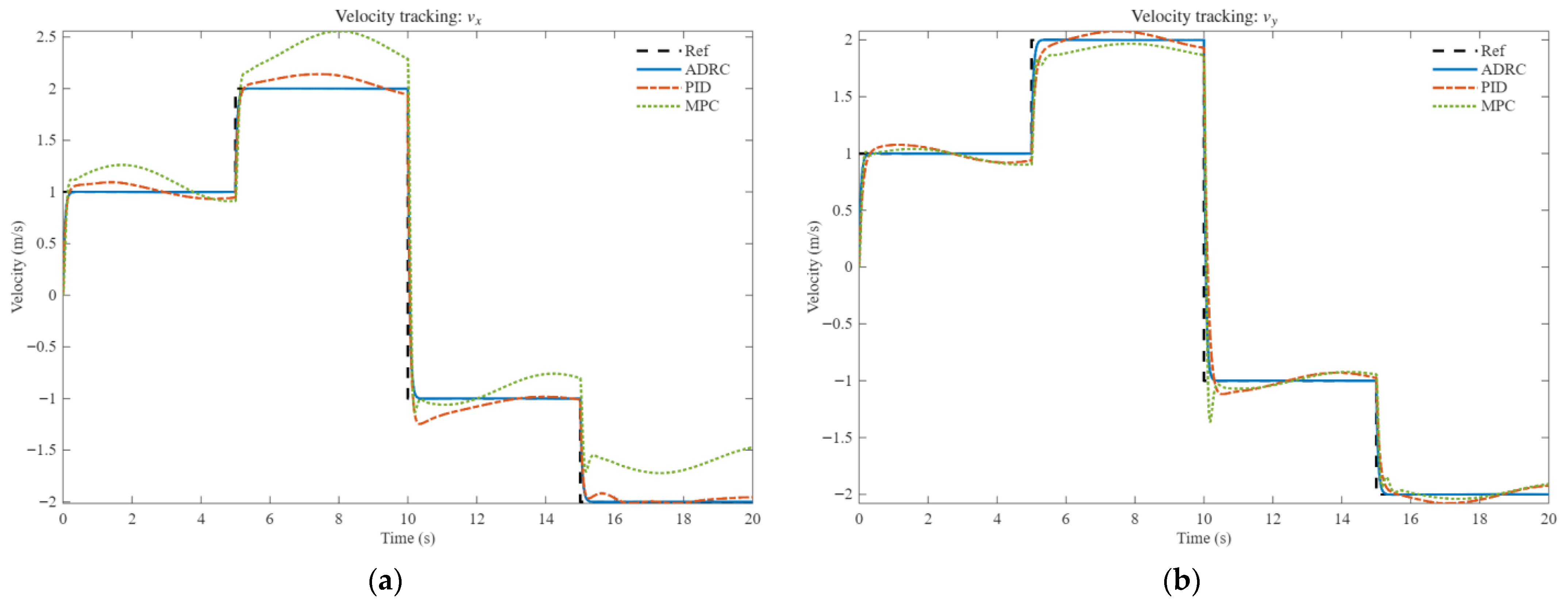
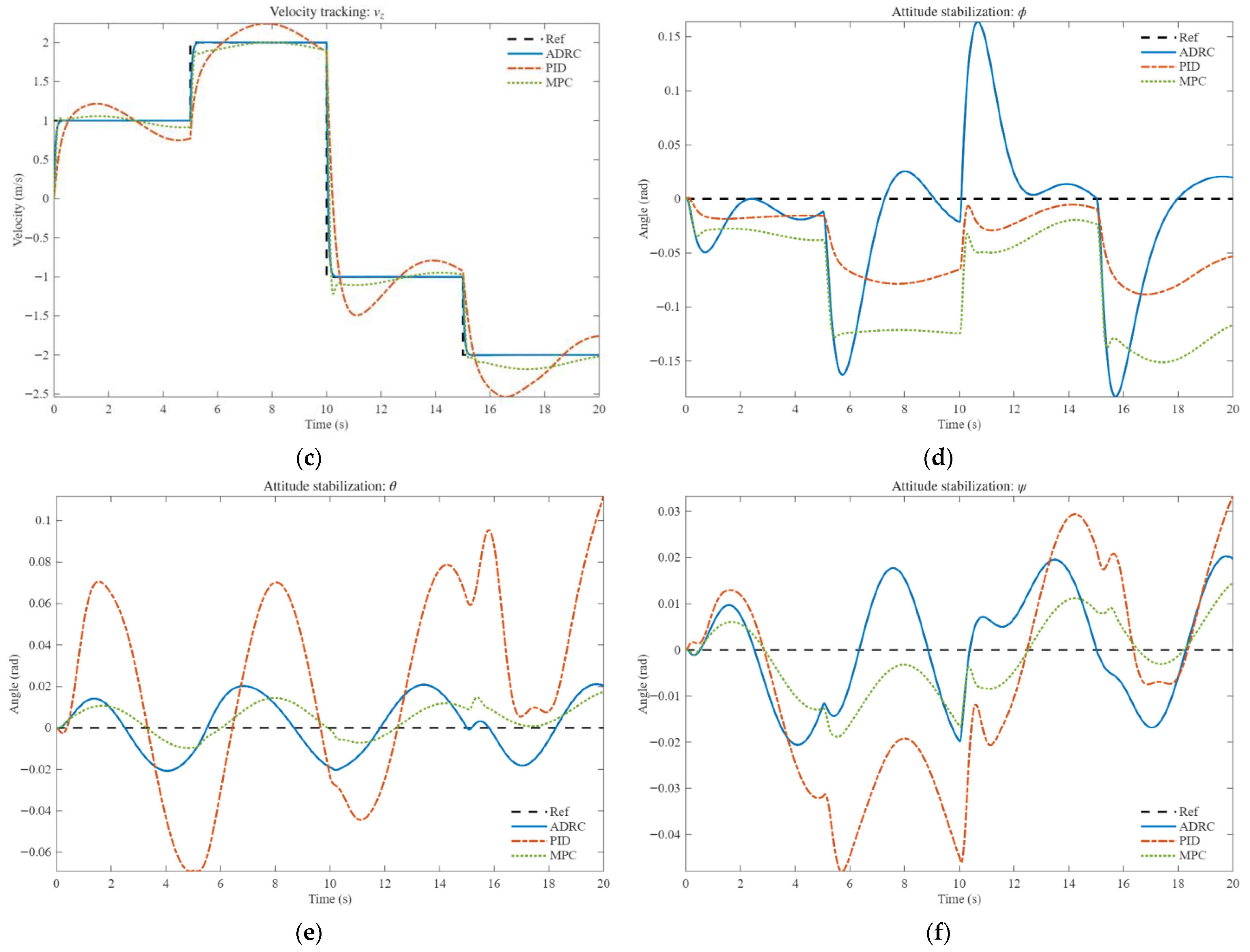
The lower-layer controller is evaluated in closed loop and is compared with a conventional PID baseline and a linear MPC controller. The simulations focus on two tasks: velocity tracking and attitude stabilization. For velocity control, time-varying step commands are applied in the translational channels. For attitude control, the reference is set to zero to represent a stabilization task. To examine disturbance rejection, sinusoidal disturbances are injected during the simulations. The same initial conditions are used for all controllers to ensure a fair comparison. The ADRC and PID parameters are listed in

Table 1. ADRC and PID parameters.

Methods	Parameters for the Attitude Controller	Parameters for the Velocity Controller
ADRC	$l_{1i}=150$$, l_{2i}=7500$$, l_{3i}=\text{125,000}$$, k_{1i}=3$$, k_{2i}=\text{2.25}$	$l_{1i}=300$$, l_{2i}=\text{22,500}$$, k_{1i}=20$
PID	$k_p=\text{800,000}$$, k_i=5000$$, k_d=\text{100,000}$	$k_p=\text{100,000}$$, k_i=5000$$, k_d=0$

, where the ADRC gains are tuned using the bandwidth-based method [30,31]. The ESO bandwidth is selected in the frequency domain to balance tracking performance, disturbance rejection, and noise sensitivity. A higher observer bandwidth typically improves disturbance estimation but may amplify measurement noise. Therefore, the bandwidth is chosen to achieve a practical trade-off. For the linear MPC controller, the sampling time is set to 0.005 s, with a prediction horizon of 100 and a control horizon of 20. The time-domain responses are presented in Figure 4. The corresponding integral of absolute error (IAE) indices for ADRC, PID, and MPC are summarized in

Table 2. IAE indices for the ADRC, PID, and MPC methods (Bold denotes the best-performing strategy).

Methods	${\mathit{v}}_{\mathit{x}}$	${\mathit{v}}_{\mathit{y}}$	${\mathit{v}}_{\mathit{z}}$	$\mathit{\phi }$	$\mathit{\theta }$	$\mathit{\psi }$
ADRC	0.30614	0.31274	0.30954	0.85030	0.23829	0.21255
PID	1.4627	1.5134	4.8503	0.86009	0.88165	0.38204
MPC	5.5458	1.4810	1.7914	1.6026	0.14381	0.14008

. The simulation runtime for each method is summarized in

Table 3. Simulation runtime for the ADRC, PID, and MPC methods (Bold denotes the best-performing strategy).

Methods	Mean Runtime (s)	Standard Deviation (s)	Min Runtime (s)	Max Runtime (s)
ADRC	5.2367	0.075477	5.1502	5.3374
PID	2.3978	0.19478	2.2104	2.6717
MPC	11.974	0.19002	11.682	12.164

. All simulations are performed on a PC with an AMD Ryzen 5 processor and 16 GB RAM using MATLAB R2025.

The time-domain results in Figure 4 show clear differences between the three controllers under the same reference steps and sinusoidal disturbances. In the velocity loops, the ADRC response follows the step commands faster and with smaller overshoot. It also shows less oscillation after each command change. The PID baseline exhibits larger transient errors and stronger oscillations, especially in the $v_z$ channel. The linear MPC response is more sensitive to disturbances and model mismatch. It yields a steady-state bias and slow recovery in the $v_x$ channel. These trends are consistent with the IAE indices in Table 2.

In the attitude loops, ADRC maintains bounded deviations and rejects the disturbance effectively. Compared with PID, ADRC achieves IAE reductions for $\theta$ and $\psi$. The IAE reductions reach about 73% for $\theta$ and about 44% for $\psi$. The MPC controller achieves the smallest IAE for $\theta$ and $\psi$ in this test, but it produces a larger error in the $\phi$ channel than ADRC and PID. Table 3 indicates that MPC has the longest runtime (mean 11.974 s), while ADRC and PID run faster, with mean runtimes of 5.2367 s and 2.3978 s, respectively. Overall, ADRC strikes a good balance between tracking performance and runtime, offering strong disturbance rejection and stable closed-loop responses while staying practical for the upper-layer training.

4.2. Obstacle-Avoidance Navigation Using Safe Reinforcement Learning

The simulation is designed to evaluate the proposed upper-layer safe reinforcement learning method for obstacle-avoidance navigation. The objective is to assess learning efficiency and safety performance. The same lower-layer ADRC is used in all cases. This choice keeps the closed-loop tracking dynamics consistent. It also ensures that the comparison focuses on the upper-layer decision module.

Four upper-layer controllers are compared in both training and validation. The first one is the proposed TD3 policy (TD3 + QP + SR). It is combined with a CBF-based QP safety filter and safety-inspired reward shaping. The second one removes the QP safety filter (TD3 + SR). It keeps the same TD3 network structure and the same reward function. The third one removes the safety-inspired reward shaping but keeps the QP safety filter (TD3 + QP), which corresponds to a typical shielded RL baseline where a nominal policy is supervised online by a safety filter. The fourth one removes both the QP safety filter and the safety-related reward terms (TD3). The key hyperparameters for RL training are shown in

Table 4. Key hyperparameters for RL training (Bold denotes that the parameters in the first row are split into multiple lines for layout).

Sample Time	Episode Horizon	Experience Buffer Size	Mini-Batch Size	Discount Factor	Target Smooth Factor
0.5 s	40 s	5 × 105	256	0.98	0.005
Learning Frequency	Policy Update Frequency	Target Update Frequency	Optimizer	Critic Learning Rate	Actor Learning Rate
2	4	2	Adam	0.0001	0.00003

. All cases share the same environment, initial conditions, sampling time, and actuator limits. Therefore, the effects of the safety filter and the safety terms in the reward can be isolated. The results provide direct evidence of the effectiveness of the proposed framework.

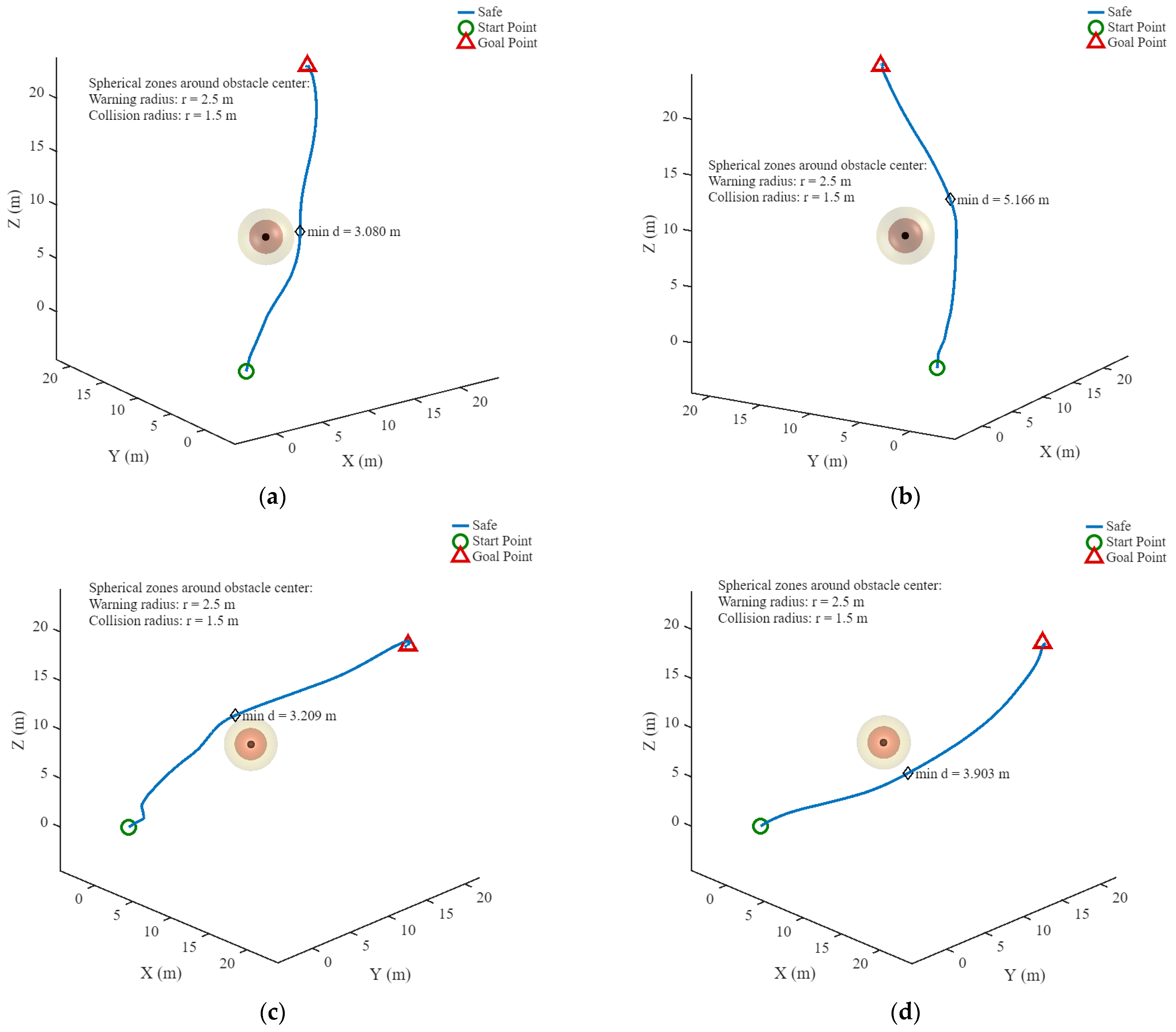
At the beginning of each episode, the desired position is randomized within the interval [15, 20] for each axis to evaluate robustness to varying goal locations in the static-obstacle setting. A static obstacle is placed at $p_{obs}={[\begin{array}{ccc}8& 8& 8.5\end{array}]}^{\mathrm{T}}$. Two safety zones are defined around the obstacle: a collision zone with radius $d_{\mathrm{collision}}=1.5 \mathrm{m}$ and a warning zone with radius $d_{\mathrm{warning}}=2.5 \mathrm{m}$. The agent outputs a 3D velocity command, and each component is bounded by [−2, 2] to match the UUV speed limits.

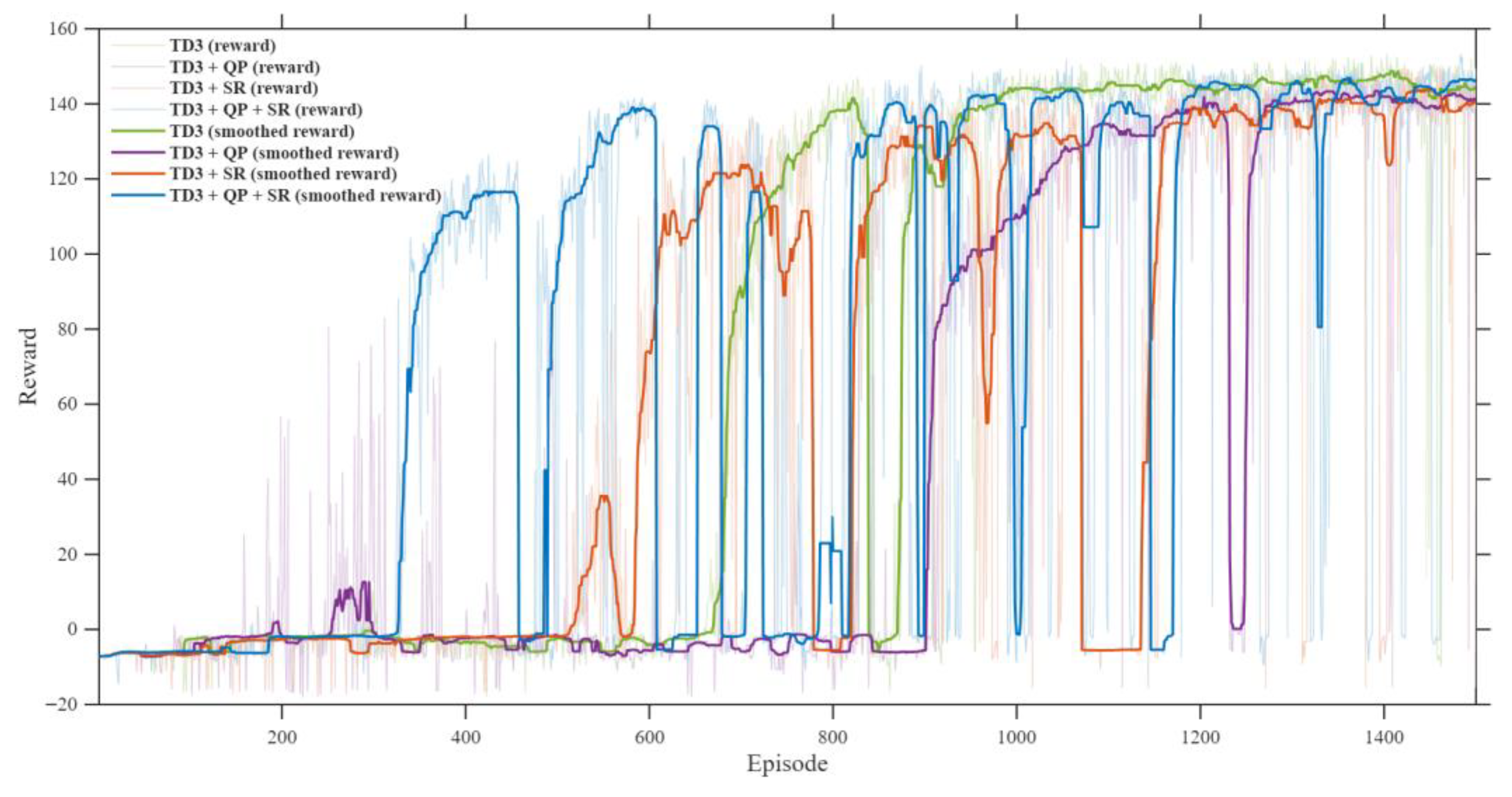
The training rewards of TD3 + QP + SR, TD3 + SR, TD3 + QP, and the TD3 baseline are compared in Figure 5. The proposed TD3 + QP + SR reaches a high reward level earlier and shows faster growth once exploration starts. Its smoothed reward rises sooner and remains high for most of the later episodes, indicating higher learning efficiency and better training stability than the other three methods.

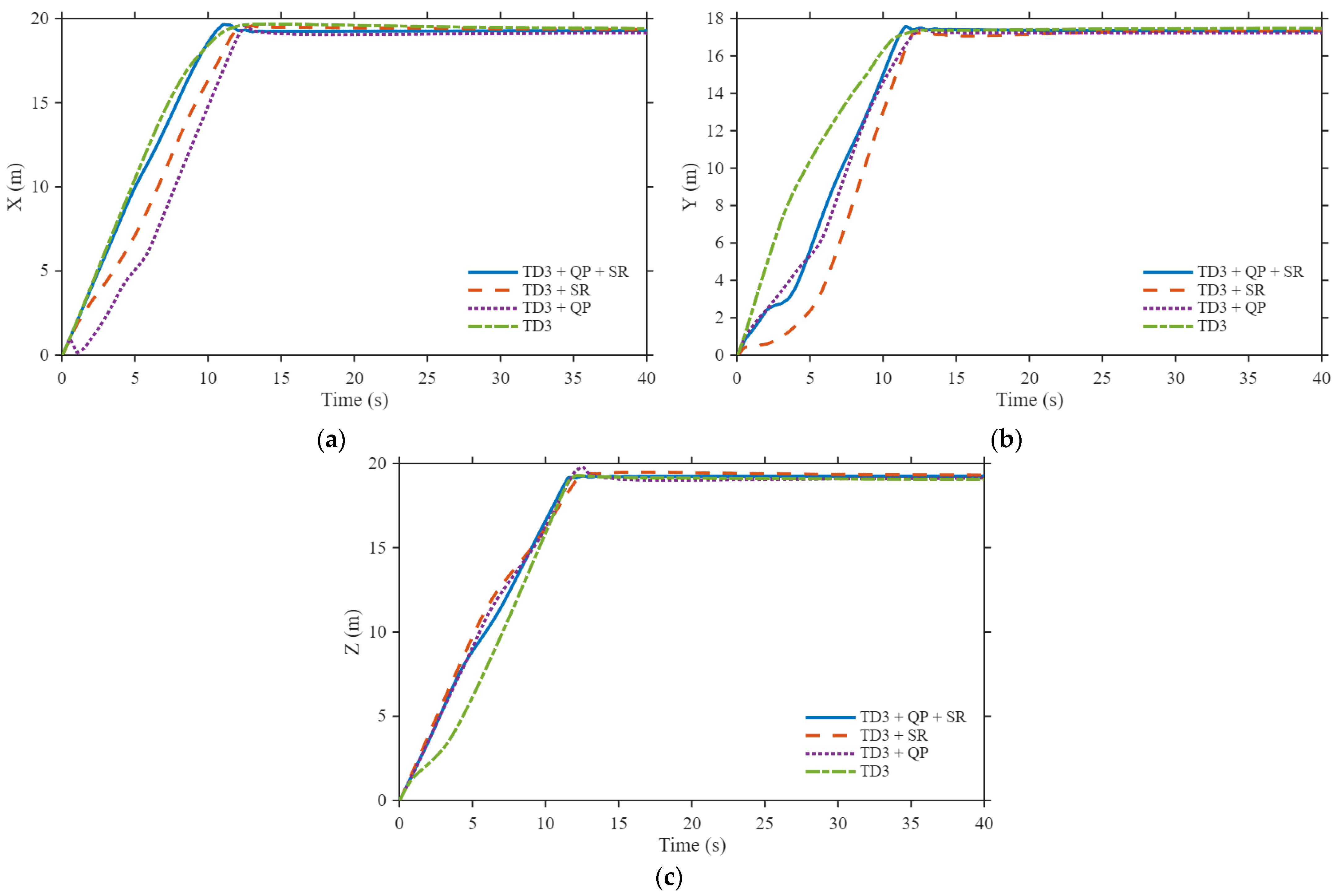
In the simulation validation stage, to avoid bias to a fixed initial condition, the UUV initial position is randomly sampled at the beginning of each episode. One representative start point is selected as ${\left[\begin{array}{ccc}19.3135& 17.3424& 19.2869\end{array}\right]}^{\mathrm{T}}$. The position responses along the x-, y-, and z-axes are shown in Figure 6. The proposed method produces more consistent responses during the navigation process. Figure 7 further visualizes the 3D obstacle-avoidance trajectories. In the legend, “safe” denotes trajectory segments that remain in the safe region. In this case, all four methods stay within the safe region. TD3 + QP + SR yields smoother and more reliable paths while maintaining a safe clearance from obstacles, compared with TD3 + SR, TD3 + QP, and TD3.

Table 5. Performance metric comparison of TD3 + QP + SR, TD3 + SR, TD3 + QP and TD3 algorithms (Bold denotes the best-performing strategy).

Algorithms	Settling Time (s)	Average IAE	Minimum Distance (m)
TD3 + QP + SR	11.393	106.991	3.080
TD3 + SR	12.027	123.263	5.166
TD3 + QP	12.710	125.763	3.209
TD3	11.556	104.102	3.903

supports these observations with quantitative metrics. TD3 + QP + SR achieves the shortest settling time 11.393 s, implying faster arrival at the goal. It also reduces the average IAE to 106.991 compared with 123.263 for TD3 + SR, which indicates better tracking accuracy. The TD3 + QP baseline attains an average IAE of 125.763 and a settling time of 12.710 s, showing that the QP safety filter alone can enforce safety but may lead to more conservative behavior without safety-inspired reward shaping. The TD3 baseline achieves a slightly lower average IAE than TD3 + QP + SR. However, the difference is small, and it comes with the key limitation that TD3 does not include an online constraint-enforcement mechanism. In contrast, TD3 + QP + SR explicitly enforces the safety constraints through the CBF-QP filter, which can modify the nominal action to keep the system within the safe set, potentially introducing a modest increase in tracking error but improving safety consistency. In addition, TD3 + QP + SR attains the smallest minimum distance 3.080 m. This indicates that, while still satisfying the safety constraints, it passes closer to the obstacle and can reach the goal more efficiently. Overall, these results suggest that the safety filter and the safety-inspired reward terms guide exploration toward feasible and safe actions, enabling faster learning and strong navigation performance.

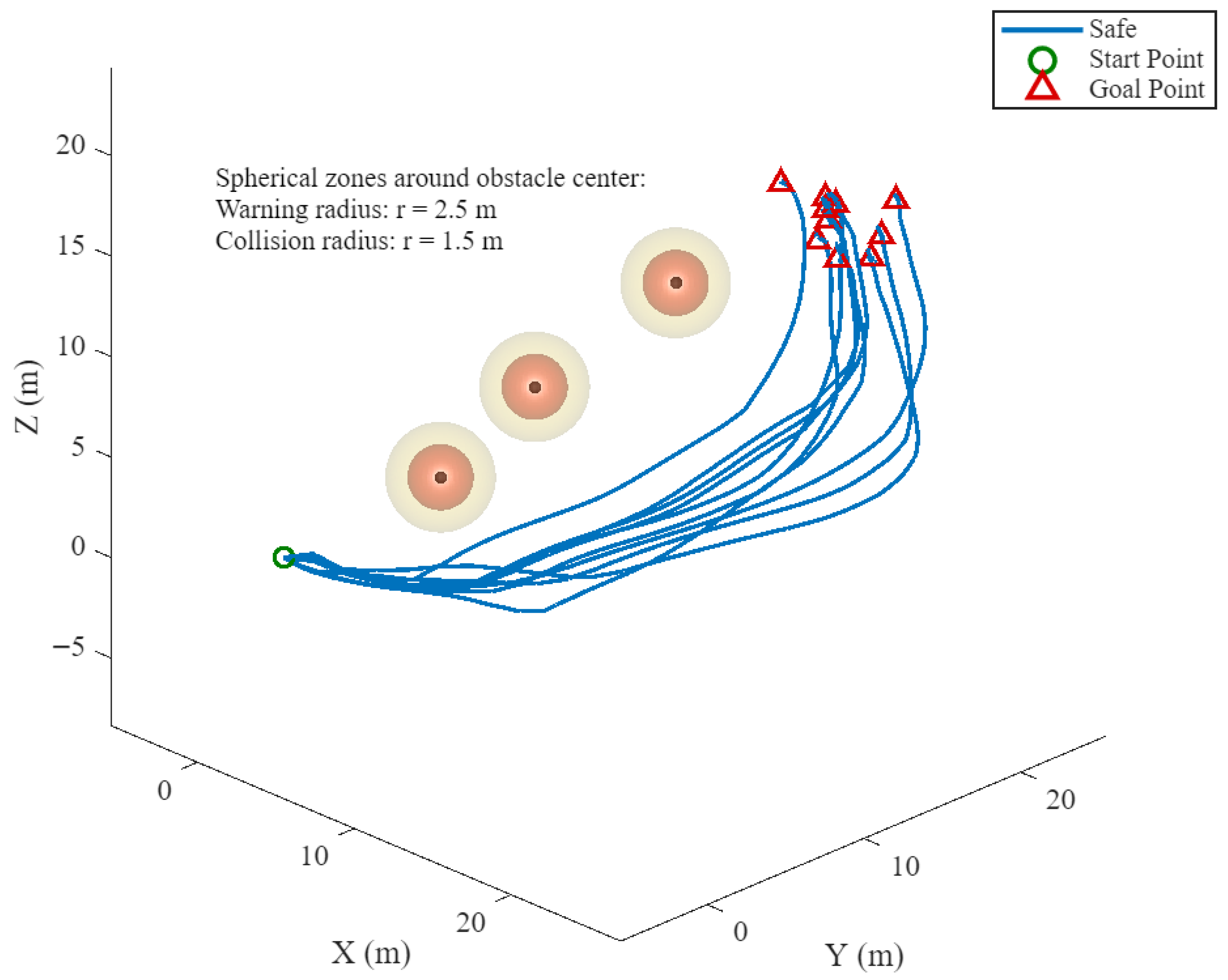
To further evaluate the applicability of the proposed method to subsea inspection scenarios with fixed structures, simulation validation is conducted in a scenario with three obstacle regions and a randomly generated goal position. The results are shown in Figure 8. Ten different goals are tested in this setting. The proposed navigation and control method can avoid the obstacles smoothly and reach the goal accurately. These results confirm that the method is general and can handle multi-obstacle and random target points.

5. Conclusions

This work presents a two-layer control framework for UUV navigation. It combines a lower-layer ADRC for robust velocity tracking and attitude stabilization with an upper-layer safe RL policy for obstacle-avoidance navigation. Two simulation studies are conducted. In the lower-layer tests, ADRC tracks time-varying step commands faster than a PID baseline and shows stronger rejection of sinusoidal disturbances. In the navigation tests, the proposed TD3 + QP + SR method improves learning efficiency and overall navigation performance compared with the ablation baselines. Under the same environment settings and the same lower-layer controller, TD3 + QP + SR achieves the shortest settling time of 11.393 s and a lower average IAE of 106.991 than TD3 + SR, and it also outperforms the TD3 + QP in terms of settling time and average IAE. It maintains a minimum obstacle distance of 3.080 m throughout the task. Although the plain TD3 baseline yields a slightly smaller IAE, it does not include an online constraint-enforcement mechanism, whereas the CBF-QP filter in TD3 + QP + SR provides explicit safety enforcement, resulting in a good trade-off among safety, efficiency, and accuracy. These results indicate that the hierarchical design improves closed-loop robustness and enables safe and efficient learning-based obstacle avoidance. This work focuses on obstacle avoidance near static structures, a typical scenario in subsea inspection tasks. In future work, we will extend the evaluation to moving obstacles and partially observable environments, and conduct experimental validation on physical platforms.

References

1. Li, J.; Zhang, G.; Jiang, C.; Zhang, W. A Survey of Maritime Unmanned Search System: Theory, Applications and Future Directions. Ocean Eng. 2023, 285, 115359. [Google Scholar] [CrossRef] [Scilit]
2. Pan, W.; Wang, Y.; Song, F.; Peng, L.; Zhang, X. UUV-assisted Icebreaking Application in Polar Environments using GA-SPSO. J. Mar. Sci. Eng. 2024, 12, 1845. [Google Scholar] [CrossRef] [Scilit]
3. Liu, S.; Ma, C.; Juan, R. AUV Obstacle Avoidance Framework Based on Event-triggered Reinforcement Learning. Electronics 2024, 13, 2030. [Google Scholar] [CrossRef] [Scilit]
4. Liu, H.; Qi, Z.; Yuan, J.; Tian, X. Robust Fixed-time H∞ Tracking Control of UUVs with Partial and Full State Constraints and Prescribed Performance under Input Saturation. Ocean Eng. 2023, 283, 115023. [Google Scholar] [CrossRef] [Scilit]
5. Er, M.J.; Gong, H.; Liu, Y.; Liu, T. Intelligent Trajectory Tracking and Formation Control of Underactuated Autonomous Underwater Vehicles: A Critical Review. IEEE Trans. Syst. Man Cybern. Syst. 2024, 54, 543–555. [Google Scholar] [CrossRef] [Scilit]
6. Antonelli, G. Underwater Robots, 3rd ed.; Springer International Publishing: Cham, Switzerland, 2014. [Google Scholar]
7. Wang, Y.; Bao, H.; Guo, C.; Williams, G.; Li, Y.; Zhang, H. An SO(3)-Based Attitude Control With Saturation Constraints for Underactuated Underwater Vehicles. IEEE Robot. Autom. Lett. 2026, 11, 1402–1409. [Google Scholar] [CrossRef] [Scilit]
8. Dong, B.; Lu, Y.; Xie, W.; Huang, L.; Chen, W.; Yang, Y. Robust Performance-Prescribed Attitude Control of Foldable Wave-Energy Powered AUV Using Optimized Backstepping Technique. IEEE Trans. Intell. Veh. 2023, 8, 1230–1240. [Google Scholar] [CrossRef] [Scilit]
9. Tang, J.; Dang, Z.; Deng, Z.; Li, C. Adaptive Fuzzy Nonlinear Integral Sliding Mode Control for Unmanned Underwater Vehicles Based on ESO. Ocean Eng. 2022, 266, 113154. [Google Scholar] [CrossRef] [Scilit]
10. Han, J. From PID to Active Disturbance Rejection Control. IEEE Trans. Ind. Electron. 2009, 56, 900–906. [Google Scholar] [CrossRef] [Scilit]
11. She, J.; Miyamoto, K.; Han, Q.L.; Wu, M.; Hashimoto, H.; Wang, Q.G. Generalized-Extended-State-Observer and Equivalent-Input-Disturbance Methods for Active Disturbance Rejection: Deep Observation and Comparison. IEEE/CAA J. Autom. Sin. 2023, 10, 957–968. [Google Scholar] [CrossRef] [Scilit]
12. Zhang, W.; Wu, W.; Li, Z.; Du, X.; Yan, Z. Three-Dimensional Trajectory Tracking of AUV Based on Nonsingular Terminal Sliding Mode and Active Disturbance Rejection Decoupling Control. J. Mar. Sci. Eng. 2023, 11, 959. [Google Scholar] [CrossRef] [Scilit]
13. Li, Z.; Liang, S.; Guo, M.; Zhang, H.; Wang, H.; Li, Z. ADRC-Based Underwater Navigation Control and Parameter Tuning of an Amphibious Multirotor Vehicle. IEEE J. Ocean. Eng. 2024, 49, 775–792. [Google Scholar] [CrossRef] [Scilit]
14. Zhao, Y.; Zhou, H.; Pan, X.; Jin, Y.; Tian, Z.; Zhao, Y. Optimized Line-of-Sight Active Disturbance Rejection Control for Depth Tracking of Hybrid Underwater Gliders in Disturbed Environments. J. Mar. Sci. Eng. 2025, 13, 1835. [Google Scholar] [CrossRef] [Scilit]
15. Wang, C.; Cai, W.; Lu, J.; Ding, X.; Yang, J. Design, Modeling, Control, and Experiments for Multiple AUVs Formation. IEEE Trans. Autom. Sci. Eng. 2022, 19, 2776–2787. [Google Scholar] [CrossRef] [Scilit]
16. Liu, T.; Huang, J.; Zhao, J. Research on obstacle avoidance of underactuated autonomous underwater vehicle based on offline reinforcement learning. Robotica 2025, 43, 194–218. [Google Scholar] [CrossRef] [Scilit]
17. Fan, Y.; Dong, H.; Zhao, X.; Denissenko, P. Path-Following Control of Unmanned Underwater Vehicle Based on an Improved TD3 Deep Reinforcement Learning. IEEE Trans. Control Syst. Technol. 2024, 32, 1904–1919. [Google Scholar] [CrossRef] [Scilit]
18. Hadi, B.; Khosravi, A.; Sarhadi, P. Deep Reinforcement Learning for Adaptive Path Planning and Control of an Autonomous Underwater Vehicle. Appl. Ocean Res. 2022, 129, 103326. [Google Scholar] [CrossRef] [Scilit]
19. Zhang, C.; Cheng, P.; Du, B.; Dong, B.; Zhang, W. AUV Path Tracking with Real-time Obstacle Avoidance via Reinforcement Learning under Adaptive Constraints. Ocean Eng. 2022, 256, 111453. [Google Scholar] [CrossRef] [Scilit]
20. Gu, S.; Yang, L.; Du, Y.; Chen, G.; Walter, F.; Wang, J.; Knoll, A. A Review of Safe Reinforcement Learning: Methods, Theories, and Applications. IEEE Trans. Pattern Anal. Mach. Intell. 2024, 46, 11216–11235. [Google Scholar] [CrossRef] [Scilit]
21. Emam, Y.; Notomista, G.; Glotfelter, P.; Kira, Z.; Egerstedt, M. Safe Reinforcement Learning Using Robust Control Barrier Functions. IEEE Robot. Autom. Lett. 2025, 10, 2886–2893. [Google Scholar] [CrossRef] [Scilit]
22. Cao, F.; Xu, H.; Ru, J.; Li, Z.; Zhang, H.; Liu, H. Collision Avoidance of Multi-UUV Systems Based on Deep Reinforcement Learning in Complex Marine Environments. J. Mar. Sci. Eng. 2025, 13, 1615. [Google Scholar] [CrossRef] [Scilit]
23. Brunke, L.; Greeff, M.; Hall, A.W.; Yuan, Z.; Zhou, S.; Panerati, J.; Schoellig, A.P. Safe Learning in Robotics: From Learning-Based Control to Safe Reinforcement Learning. Annu. Rev. Control Robot. Auton. Syst. 2022, 5, 411–444. [Google Scholar] [CrossRef] [Scilit]
24. Stooke, A.; Achiam, J.; Abbeel, P. Responsive Safety in Reinforcement Learning by PID Lagrangian Methods. In Proceedings of the 37th International Conference on Machine Learning (ICML 2020), Vienna, Austria, 12–18 July 2020. [Google Scholar]
25. Chow, Y.; Nachum, O.; Duenez-Guzman, E.; Ghavamzadeh, M. A Lyapunov-Based Approach to Safe Reinforcement Learning. In Proceedings of the 32nd International Conference on Neural Information Processing Systems (NeurIPS 2018), Montréal, QC, Canada, 3–8 December 2018. [Google Scholar]
26. Wabersich, K.P.; Zeilinger, M.N. A Predictive Safety Filter for Learning-Based Control of Constrained Nonlinear Dynamical Systems. Automatica 2021, 129, 109597. [Google Scholar] [CrossRef] [Scilit]
27. Cheng, R.; Orosz, G.; Murray, R.M.; Burdick, J.W. End-to-End Safe Reinforcement Learning through Barrier Functions for Safety-Critical Continuous Control Tasks. In Proceedings of the AAAI Conference on Artificial Intelligence (AAAI 2019), Honolulu, HI, USA, 27 January–1 February 2019. [Google Scholar]
28. Zheng, Q.; Gao, L.Q.; Gao, Z. On Validation of Extended State Observer through Analysis and Experimentation. J. Dyn. Syst. Meas. Control 2012, 134, 024505. [Google Scholar] [CrossRef] [Scilit]
29. Zheng, Q.; Chen, Z.; Gao, Z. A Practical Approach to Disturbance Decoupling Control. Control Eng. Pract. 2009, 17, 1016–1025. [Google Scholar] [CrossRef] [Scilit]
30. Gao, Z. Scaling and Bandwidth-parameterization based Controller Tuning. In Proceedings of the 2003 American Control Conference (ACC 2003), Denver, CO, USA, 4–6 June 2003. [Google Scholar]
31. Jin, H.; Song, J.; Lan, W.; Gao, Z. On the characteristics of ADRC: A PID interpretation. Sci. Chin. Inf. Sci. 2020, 63, 209201. [Google Scholar] [CrossRef] [Scilit]
Figure 1. Schematic diagram of the UUV.
Jmse 14 00425 g001
Figure 2. Two-layer control framework for the UUV.
Jmse 14 00425 g002
Figure 3. Network architecture.
Jmse 14 00425 g003
Figure 4. Time-domain responses for the lower-layer closed-loops: (a) Velocity tracking for the v x loop. (b) Velocity tracking for the v y loop. (c) Velocity tracking for the v z loop. (d) Attitude stabilization for the φ loop. (e) Attitude stabilization for the θ loop. (f) Attitude stabilization for the ψ loop.
Jmse 14 00425 g004aJmse 14 00425 g004b
Figure 5. Training results of TD3 + QP + SR, TD3 + SR, TD3 + QP and TD3 algorithms.
Jmse 14 00425 g005
Figure 6. Position responses along x-, y-, and z-axes: (a) Position responses along x-axis. (b) Position responses along y-axis. (c) Position responses along z-axis.
Jmse 14 00425 g006
Figure 7. Comparison of 3D obstacle-avoidance trajectories. (a) 3D obstacle-avoidance trajectory of TD3 + QP + SR algorithm; (b) 3D obstacle-avoidance trajectory of TD3 + SR algorithm; (c) 3D obstacle-avoidance trajectory of TD3 + QP algorithm; (d) 3D obstacle-avoidance trajectory of TD3 algorithm.
Jmse 14 00425 g007
Figure 8. Obstacle-avoidance trajectory in the multi-obstacle scenario.
Jmse 14 00425 g008