Study on Single-Point Mooring Cables for Stereoscopic Environmental Monitoring in the Natural Gas Hydrate Area of the South China Sea

Abstract

Safe exploitation of the marine natural gas hydrate (NGH) resource is essential to meet the demand of the future energy requirement. To enable real-time monitoring of methane leakage during the production test of NGH, an ocean stereoscopic monitoring system based on underwater single-point mooring structure is developed, which supports in situ monitoring of marine environment at the sea-air interface, the euphotic zone, and the seabed boundary layer. Numerical simulations were conducted to evaluate the effect of mooring configuration, cable lengths, and buoyancy settings on the mooring stability of the system against the current and waves. Based on the simulation result, an optimized segmented inverse-catenary mooring configuration is developed to achieve a balance between the performance and cost. The designed submersible relay buoy isolates the upper dynamic S-shaped cable from the lower static straight electro-optical-mechanical (EOM) cable, thereby improving system stability. The monitoring system based on the optimized mooring structure is successfully deployed at the NGH zone in the northern South China Sea at the water depth of 1330 m confirming its working stability in harsh sea conditions.

1. Introduction

Natural gas hydrate (NGH) is considered as a promising future green energy source due to its vast reserves and friendliness to the environment [1,2,3]. However, its exploitation poses significant risks. Disturbances such as rapid sea-level decline and tectonic activity (e.g., earthquake) can destabilize hydrate-bearing formations, causing NGH to decompose rapidly, which releases large amounts of methane into the ocean [4,5,6]. This may intensify the greenhouse effect, trigger submarine landslides, and disrupt marine ecosystems [7,8,9]. Therefore, a comprehensive assessment of environmental risks is essential before the commercial NGH exploration. Special attention should be given to stereoscopic monitoring on the methane leakage—across the seabed, water column, and sea-air interface—to ensure safe and sustainable utilization of NGH resources.

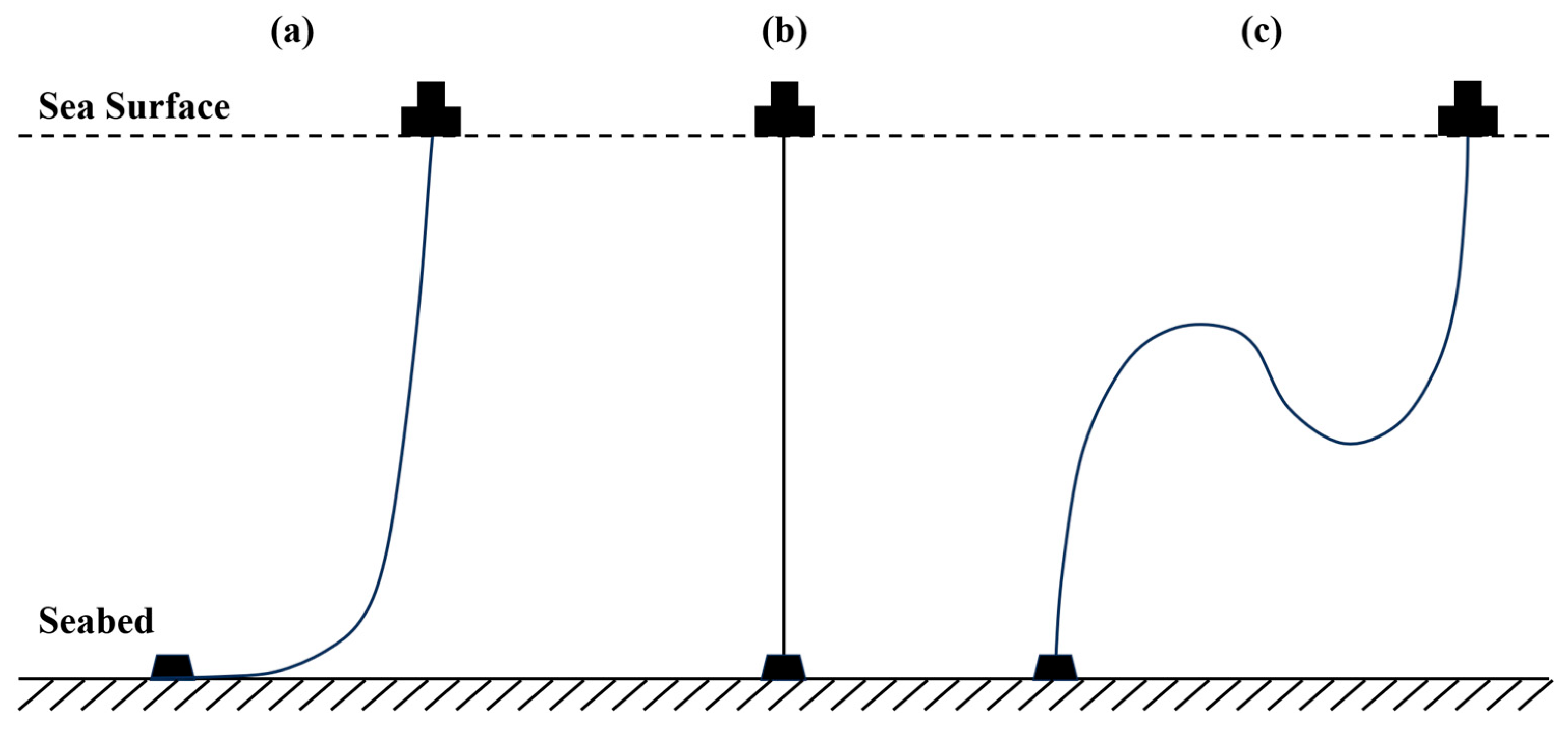
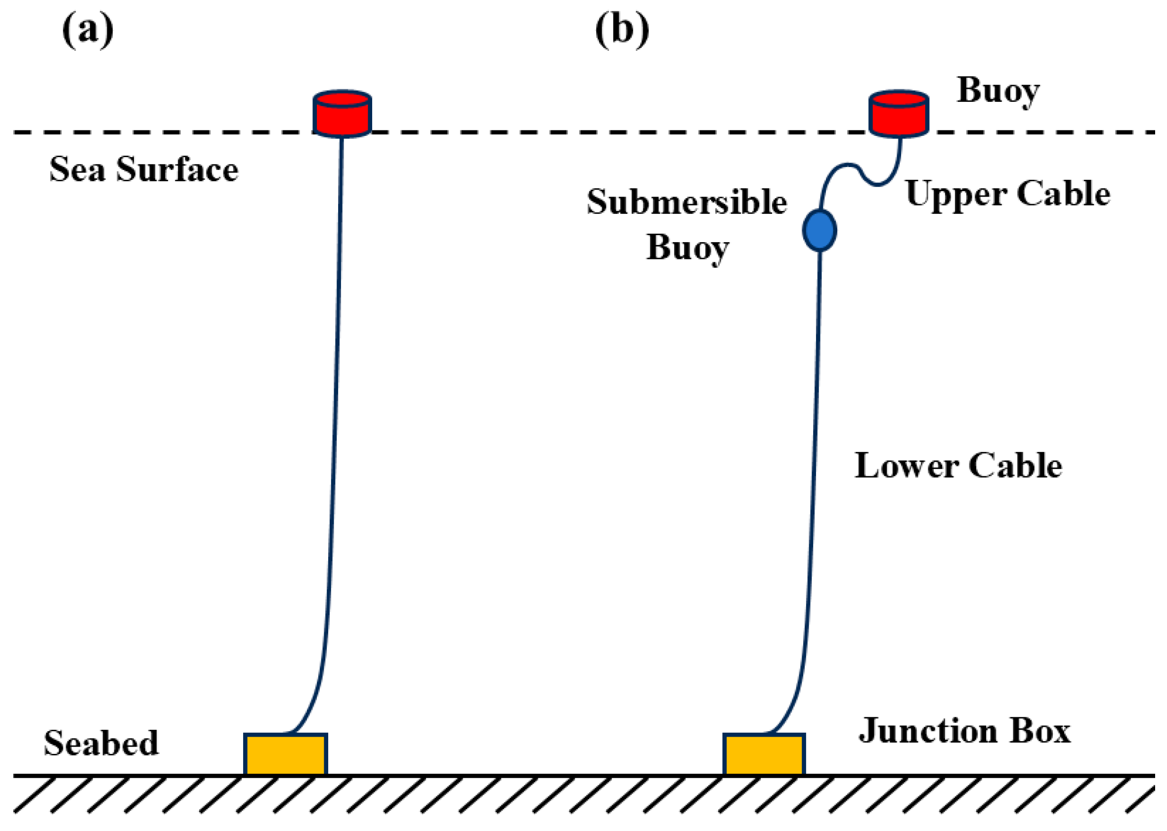
The stereoscopic monitoring system based on single-point mooring cables is widely applied for long-term, in situ marine environmental observation [10]. As shown in Figure 1, it is composed of buoys, mooring cables, and seabed observation nodes, based on which coordinated data collection and transmission can be realized. The system has a low cost and strong environmental adaptability. The stability of the system mainly depends on the configuration of underwater mooring structure, which must balance the ambient disruption. Currently, there are three types of mooring structures, namely, the chain-catenary, semi-taut, and inverse-catenary structures (see Figure 1).

The chain-catenary structure fixes the buoy by a suspended anchor chain, as shown in Figure 1a, achieving stable mooring through the balance of the chain’s weight and the buoy’s buoyancy. This mooring structure offers several advantages, including its simplicity on the structure and tolerance to water depth uncertainty or changes. However, its application is limited in deep waters due to increased design complexity and self-weight, as well as the cost [10]. The Catenary Anchor Leg Mooring (CALM) system is a widely adopted offshore mooring solution that ensures stable positioning of floating facilities by using chain-catenary structure. The initial design of the CALM system was simple, adopting buoys and anchor chains to moor tankers at the fixed location. It serves as an offshore refueling station. As offshore exploration moved into deeper waters, the CALM system evolved rapidly in the 1990s, which was applied at the water depths over 1000 m [11,12,13]. The CALM system was widely used in Nigeria, Brazil, Malaysia, and the North Sea, proving effective in diverse offshore settings [14,15,16,17].

The semi-taut mooring structure, as shown in Figure 1b, is an improved design based on the chain-catenary structure, which adopts anchor chains at both ends of the structure, and elastic synthetic cables such as nylon, polyester, polypropylene, and polyolefin in between [10]. The Woods Hole Oceanographic Institution (WHOI) developed the ‘GUMBY’ hose and subsurface monitoring system using the semi-taut mooring structure. In the system, hydrophones were used to investigate the activity of whales [18]. Ocean Observatories Initiative (OOI) deployed several Coastal Surface Moorings. The system includes a buoy powered by solar power and wind, a near surface detecting node located at the water depth of 7 m, and a seabed node, which are connected by electro-optical-mechanical (EOM) cables. This monitoring system has the ability to operate at water depths of up to 450 m [19,20]. Semi-taut mooring systems are also widely used in floating offshore wind turbines (FOWTs) [21,22].

As shown in Figure 1c, the inverse-catenary mooring system forms a S-curved configuration, which is realized by installing buoyancy units on the cable, or using cables with varying densities. The S-curved configuration effectively offsets the impact from the current and waves and reduces fatigue damage to the mooring cables on extreme sea conditions. Also, it extends the operational depth of single-point mooring systems to several thousand meters [10]. The inverse-catenary mooring system is widely used in deep-sea environments for meteorological, optical, ecological, and seismic monitoring. The Monterey Bay Aquarium Research Institute (MBARI) developed the MBARI Ocean Observatory System (MOOS) for the water depth of 4000 m, which connects surface buoy to seafloor node via a single EOM cable. Buoyancy units are used to produce a large S-curved shape [23,24]. The CSnet company developed the Offshore Communications Backbone (OCB) monitoring system with the inverse-catenary mooring structure, which is deployed at the water depth of 1000~2800 m [25,26]. The system is designed to monitor seafloor pressure and analyze the impact of tsunamis caused by submarine earthquakes [27,28,29]. The Chinese Academy of Sciences (CASs) developed the Mooring Buoys Observation System for Benthic with electro-optical-mechanical Cable (MBOSBC), which also incorporates an inverse-catenary mooring system with a zero-gravity cable, to support marine environmental observations in the South China Sea [30].

As a critical component of single-point mooring systems, the underwater dynamic cable, which is designed to withstand continuous mechanical bending due to environmental loads, plays a key role in determining the system’s stability and safety under complex sea conditions. Therefore, studying their configurations and hydrodynamic behavior is essential for reliable deep-sea observation systems. Paul et al. developed lightweight synthetic fiber-reinforced mooring cables and stretchable rubber EOM cable elements for the MOOS and evaluated its performance in extreme storms [31]. Grosenbaugh et al. designed a synthetic fiber-reinforced EOM cable and investigated its static and dynamic responses of moorings with low-modulus nylon or polyester fibers at water depths of 1800 m, 3000 m, and 5000 m [32]. Yu et al. provides design criteria for a single-point mooring system with a buoy, EOM cable, and benthic node. The environmental load of the buoy and the mooring hydrodynamic force of EOM were calculated, and the hydrodynamic force needed for the system under extreme marine conditions was thoroughly analyzed [33]. Han et al. compared the following two inverse-catenary mooring designs: segmented mooring using a single subsurface float (SSF) with an “S-tether” positioned above it, and integrated S-shaped mooring without SSF. The study indicates that the lengths of mooring cables, buoyancy sections, and snubber hose are important parameters influencing the stability of underwater mooring systems [34]. Bach-Gansmo et al. evaluated the performance of taut compliant and catenary mooring systems for FOWTs using experiments and simulations and highlighted the impact of mooring line angle and line pretension on dynamic response [35]. Amaechi et al. analyzed submarine hoses attached to a CALM buoy and moored by six mooring lines in a water depth of 23.0 m using a coupled dynamic model built in OrcaFlex, focusing on how hydrodynamic loads and flow angles affect the structural behavior of the hoses [36]. Touzon et al. conducted a numerical analysis of three well-known mooring design approaches applied to a floating wave energy converter moored by four catenary lines, evaluating them based on total mooring mass, required footprint, as well as the design line tension and structure offset [37].

NGH reservoirs in the South China Sea are typically located at sea depths exceeding 1000 m. Since EOM cables close to the junction box are not suitable for continuously contacting the seabed as is the case in the chain-catenary structure shown in Figure 1a, and the semi-taut mooring structure has a limited deployment water depth, therefore, a stereoscopic observation system based on the inverse-catenary mooring type for long-term, real-time deep-sea environmental monitoring needs to be developed. To address the scientific challenge of optimizing underwater mooring configurations for deep-water environments, which involves balancing minimized mooring tension, cost-effectiveness, and deployment flexibility, this study presents an Ocean Stereoscopic Monitoring System (GOSMS) based on the inverse-catenary mooring structure. The hydrodynamic performance of the mooring system considering changing of the mooring structure, cable length, and buoyancy setting is investigated via a detailed numerical simulation, with the optimized parameter being determined. The reliability of the designed system is confirmed by offshore deployment of the fabricated GOSMS at the sea depth of 1330 m in the “Shenhu” NGH area in the South China Sea.

The main novel contributions of this study are as follows: (1) a long-term independently operable GOSMS is developed. It establishes a communication architecture with redundant and complementary optical fibers, electrical cables, and acoustic transmission to enhance data delivery reliability. (2) A segmented inverse-catenary mooring configuration is optimized to achieve comprehensive improvements in dynamic stability, shape adaptability, and economic efficiency. (3) A technical framework for integrated multi-level monitoring of the marine environment is proposed, which enables real-time monitoring of methane content at multiple levels, such as the sea-air interface, the euphotic zone, and the seabed in the NGH area.

2. Materials and Methods

In this section, the mechanical design of GOSMS is introduced, the optimization method of underwater single-point mooring cables is discussed, and the basic situation of the offshore experiment is explained. In the hydrodynamic simulation of the mooring cable, this paper investigates the theories related to the hydrodynamic characteristics of the mooring cables and clarifies the tension calculation method of such cables. Based on the comprehensive optimal criterion of minimum tension, cost constraints and deployment flexibility, the influencing factors of mooring stability are discussed, and an optimized segmented inverse-catenary mooring configuration is formed and verified for reliability.

2.1. Mechanical Design

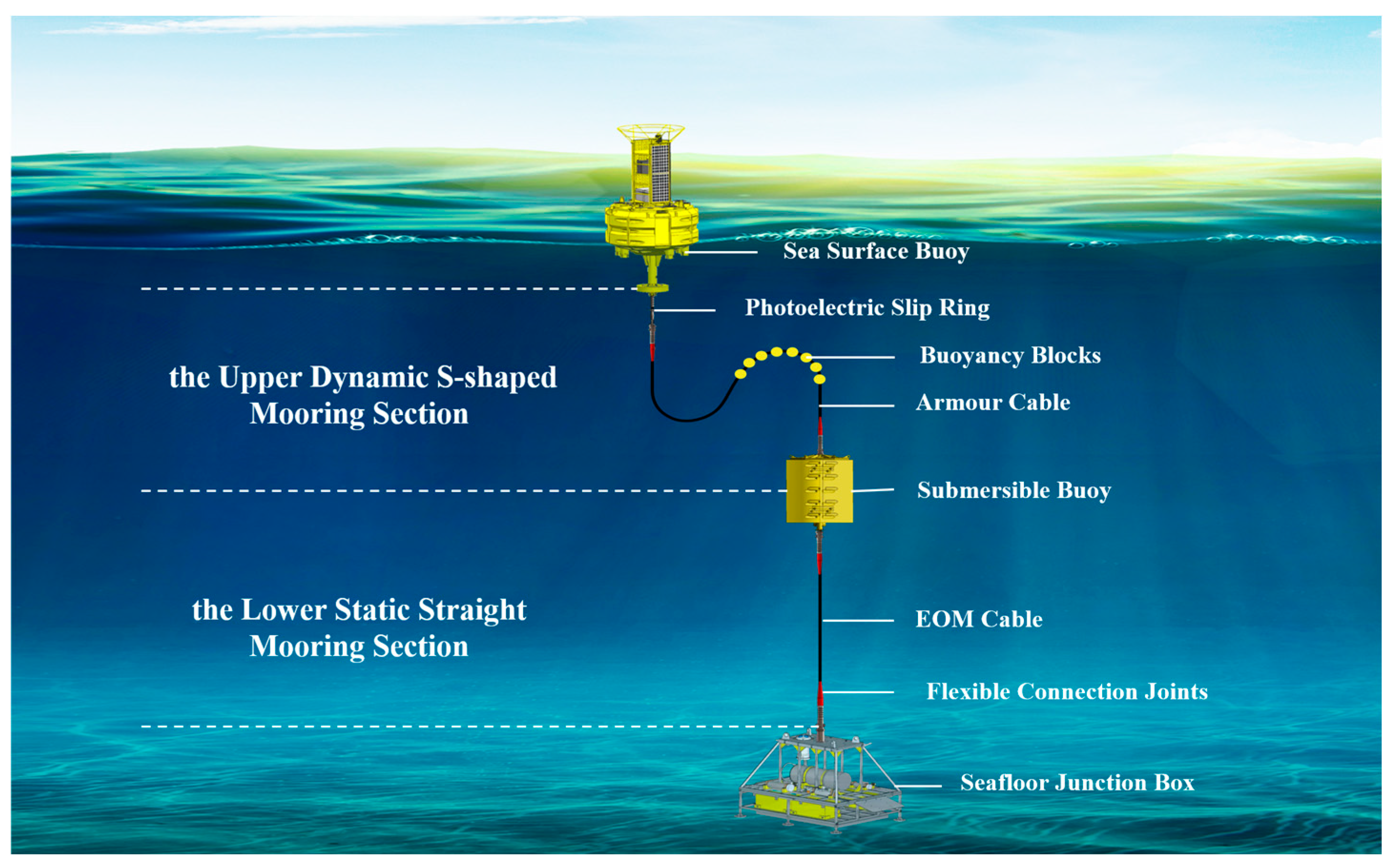
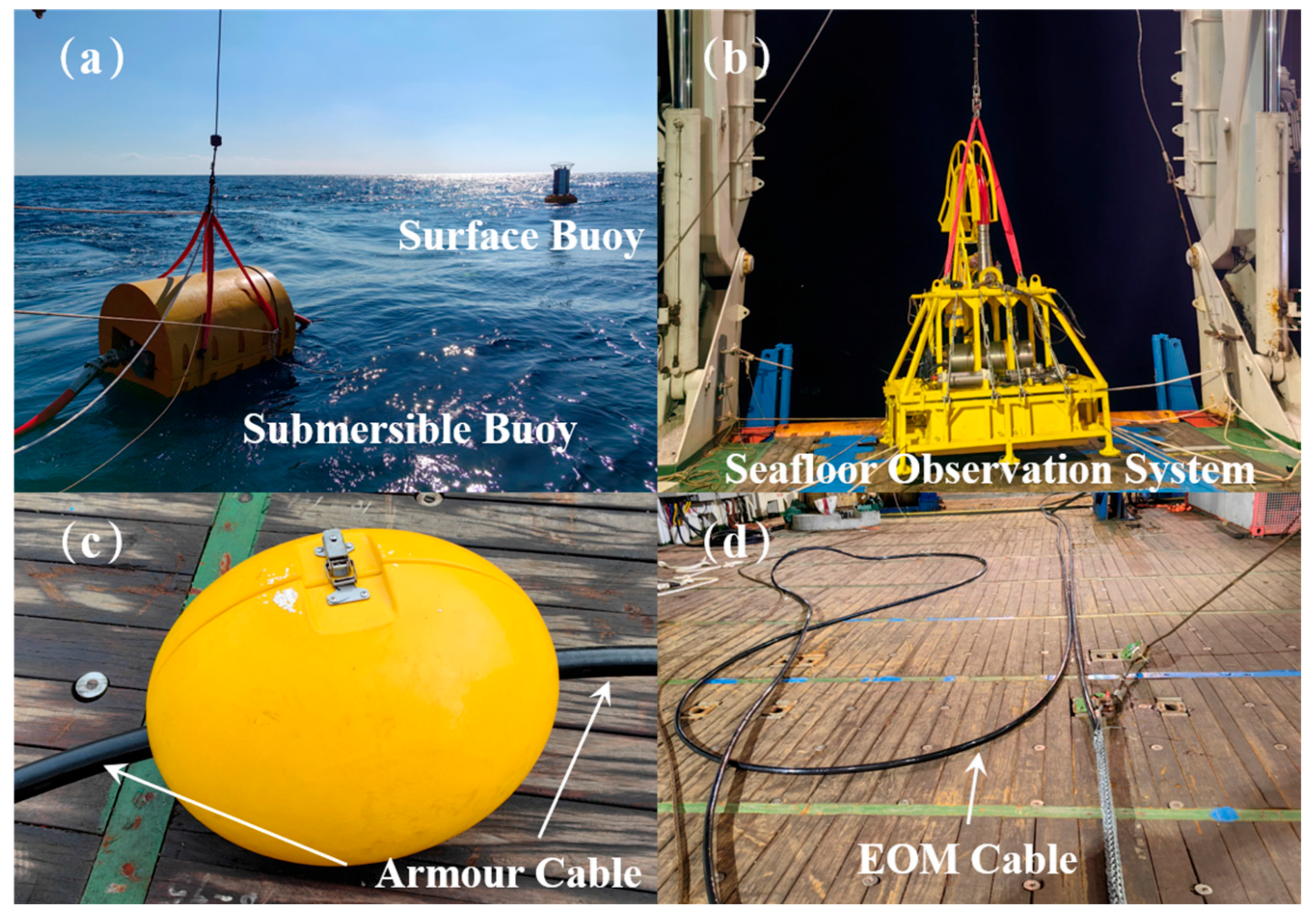
The designed GOSMS consists of a buoy, the power and communication transmission EOM cable, submersible rely buoy, and a monitoring station in a junction box on the sea floor (see Figure 2). This system enables real-time monitoring of the environmental impacts of deep-sea resource exploitation, with a focus on stereoscopic detection of methane leakage in NGH areas.

The buoy at the sea surface is primarily composed of buoy body, power supply unit, data acquisition and transmission unit, and the anchor positioning unit at the bottom. The main frame of the buoy, which has a diameter of 3.0 m, is built with a 316 L stainless steel. Polyurethane foam and polyethylene (PE) are adopted as buoyancy materials. The junction box on the seafloor has a dimension of 2.0 m × 1.9 m × 2.2 m and the weight of 3.75 t in water. It is composed of an electronic cabin, a landing unit (with ballast), and environmental monitoring sensors. The junction box acts as the anchor point that fixes the entire monitoring system on the seafloor. It is also the controlling center that guarantees the long-term operation of the system. The submersible buoy is positioned near the sea surface, which is installed with environmental monitoring sensors and the acoustic communication unit. An armored cable is used to connect the buoy and the submersible buoy, and a regular EOM cable is adopted to connect the submersible buoy to the junction box, enabling bidirectional transmission of power and data between these three sensing nodes. For the armored cable, numbers of bouncy blocks are adopted to regulate the congregation of the cable.

Various underwater sensors, including methane detectors (Aeris Ultra sensor, Aeris Technologies, Inc., Hayward, CA, USA; Contros HydroC^TM CH₄ sensor, -4H-JENA Engineering GmbH, Jena, Germany; METS CH₄ sensor, Franatech GmbH, Berlin, Germany) and carbon dioxide detectors (Contros HydroC^TM CO₂ sensor, -4H-JENA Engineering GmbH, Jena, Germany), Acoustic Doppler Current Profiler (ADCP, Teledyne RD Instruments, San Diego, CA, USA), Conductivity-Temperature-Depth (CTD, Sea-Bird Electronics, Inc., Bellevue, WA, USA), and a high-definition seabed camera (South China Sea Institute of Oceanology, Chinese Academy of Sciences, Guangzhou, China), are installed at the buoys and the junction box. These sensors enable comprehensive monitoring of environmental parameters across the sea-air interface, the euphotic zone, and the seabed boundary layer in the NGH areas.

This system employs a redundant and complementary communication method utilizing optical fibers, electrical cables, and acoustic transmission to enhance data delivery reliability. Firstly, communication between the buoy and the shore station utilizes Iridium or Beidou satellite. The data transmission frequency is adjustable based on needs. Secondly, communication between the sea surface buoy and the submersible buoy primarily relies on an armored cable using the RS485 protocol (Electronic Industries Association, EIA, Arlington County, VA, USA). Given the vulnerability of the upper dynamic cable in complex hydrodynamic conditions, an acoustic communication device serves as a backup on the submersible buoy. Thirdly, the submersible buoy and seafloor junction box are connected via the EOM cable, utilizing dual-channel communication for both optical and electrical modes. The primary communication is through optical fiber, with a transmission rate of 1000 Mbps, while RS485 electrical communication serves as a backup.

2.2. Numerical Simulation

For GOSMS deployed in the deep-sea NGH areas of the South China Sea, as is introduced previously, the inverse-catenary mooring structure is applied. In the system, the submersible buoy is adopted to effectively buffer the influence of upper water layer disturbances on the overall underwater mooring system. The hydrodynamic performance of the mooring structure is investigated through numerical simulation, and the optimized mooring configuration is proposed.

2.2.1. Simulation Method

In this study, the commercial software OrcaFlex (Version 11.4b) was employed to conduct hydrodynamic simulation of underwater single-point mooring cables, which adopts the finite element (FE) method, and the Lumped Mass model is applied to establish the mechanical analysis framework for cables [38,39,40,41]. This approach converts the distributed load acting on each cable element into equivalent nodal (mass point) loads and formulates the following motion equation for each node:

$$F\left(t\right)=M\ddot{X}+C\dot{X}+KX$$

(1)

where F(t) is the hydrodynamic exciting force vector of the system, M is the nodal mass matrix, C is the damping coefficient matrix at each node, K is the stiffness matrix, X is the motion vector, $\dot{X}$ is the velocity vector, and $\ddot{X}$ is the acceleration vector. With determined boundary conditions applied, the displacement X of each mass point in the submarine cables can be calculated, leading to the determination of node motion and the overall dynamic behavior of the cable.

The hydrodynamic loads exerted on each node of the submarine cables can be calculated by the Morison equation [42,43]:

$$F=C_{M}V{a}_f+{\displaystyle \frac{1}{2}}\rho C_{D}A\left|v_f\right|v_f$$

(2)

where F is the fluid force (per unit length) on the body, C_M is the inertia coefficient for the body, V is the mass of fluid displaced by the body, a_f is the fluid acceleration relative to earth, $\rho$ is the density of fluid, C_D is the drag coefficient for the body, A is the drag area, and v_f is the fluid velocity relative to earth.

The calculation of forces and moments is performed at each node step by step. Initially, the tensions in the cables are calculated. This involves computing the distance (and its rate of changes) between the nodes at the end of the segments, as well as the segment axial direction Sz, the unit vector in the direction joining the two nodes. The tension in the axial spring-damper at the center of each segment in the vector, in direction Sz, whose magnitude is given by the effective Te.

$$T_e=T_w+(p_o{a}_o-p_i{a}_i)$$

(3)

where T_w is the wall tension of the cable; p_i and p₀ are the internal pressure and external pressure, respectively; a_i and a₀ are the internal and external cross sectional stress areas, respectively.

2.2.2. Modeling of the Sea Condition

(1)

Ideal sea condition

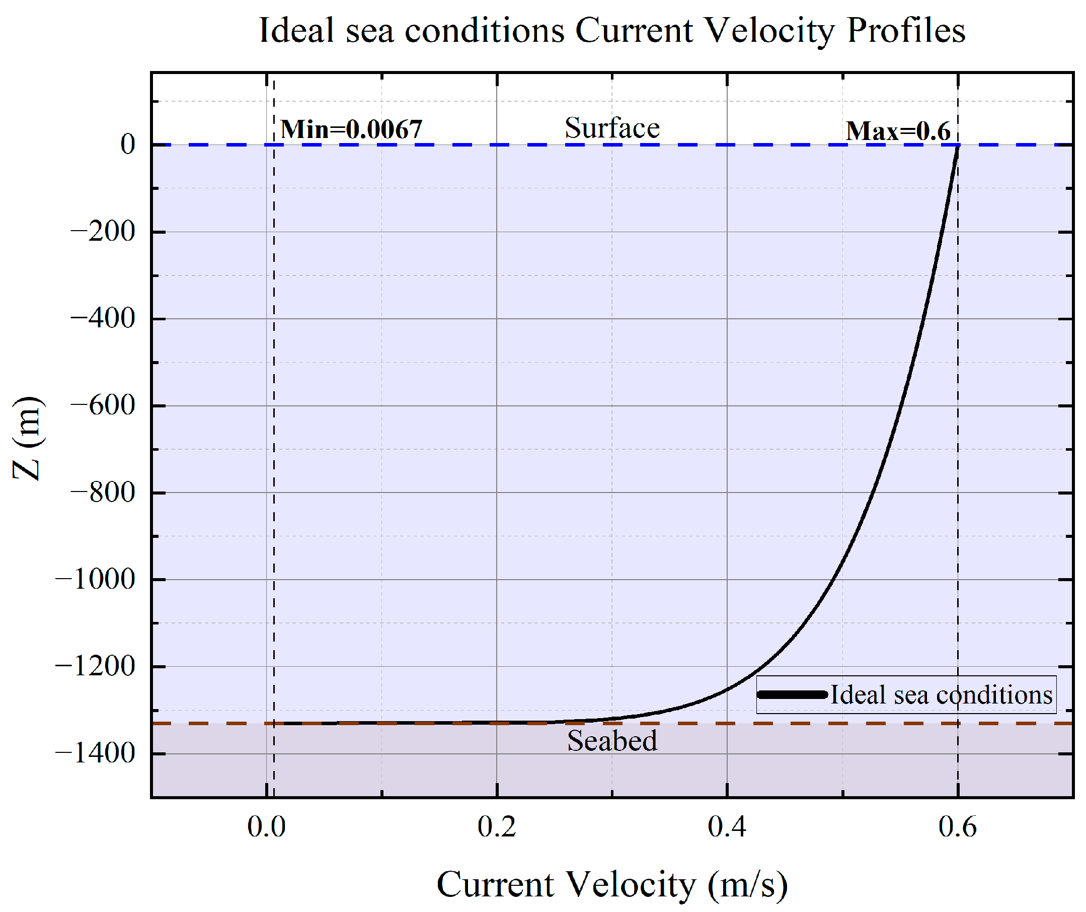
In the simulation, the density and the kinematic viscosity are set to 1025 kg/m³ and 1.350 × 10⁻⁶ m²/s, respectively. Here, an ideal sea condition based on the power-law-based current model is proposed as a standard sea condition in order to investigate the hydrodynamic performance of the mooring structure with various settings. A power-law-based current model that describes the current is proposed, as shown in Figure 3. This model assumes that the current velocity decays exponentially with depth, which approaches the characteristic current condition commonly observed in natural marine environments and is therefore widely applied for modeling the realistic marine flow field distributions [44]. However, this model has the following two limitations: (1) it does not account for extreme events (e.g., typhoon-induced currents) or seasonal variations in current direction/magnitude, which may affect mooring stability under non-ideal conditions; (2) the power-law exponent is fixed in this study, while real-world currents may exhibit depth-dependent exponent variations. Future work will validate this model against long-term observational data to improve its representativeness. The velocity S at location (X, Y, Z) is given by

$$S=S_b+(S_f-S_b){\left[{\displaystyle \frac{Z-Z_b}{Z_f-Z_b}}\right]}^{1/p}$$

(4)

where S_b is the current velocity near the seabed, S_f is the current velocity at the still water level (a theoretical static sea surface without waves or tidal variations), p is the power law exponent, Z_f is the Z coordinate of the still water level Z, and Z_b is the Z coordinate of the seabed directly below (X, Y).

In the ideal sea condition, the maximum current velocity is set to 0.6 m/s, with a power law exponent (p in Equation (4)) of 7, and the current along the horizontal direction as shown in Figure 3. Furthermore, the wave height at the sea surface is set to 2 m with the period of 7 s.

(2)

Average and Extreme Sea Conditions

The average and extreme sea conditions are applied to examine the safety of the developed mooring system based on the historical measurement from a mooring system deployed in the sea trial area (SH-C-MX03-2020, from 23 November 2020 to 13 May 2022) and supplemented with data from the third-generation wave model Wavewatch III developed by National Oceanic and Atmospheric Administration (NOAA) and National Centers for Environmental Prediction (NCEP) [45]. The average sea condition is the monthly mean current velocity, while the extreme sea condition is characterized by the monthly maximum current velocity.

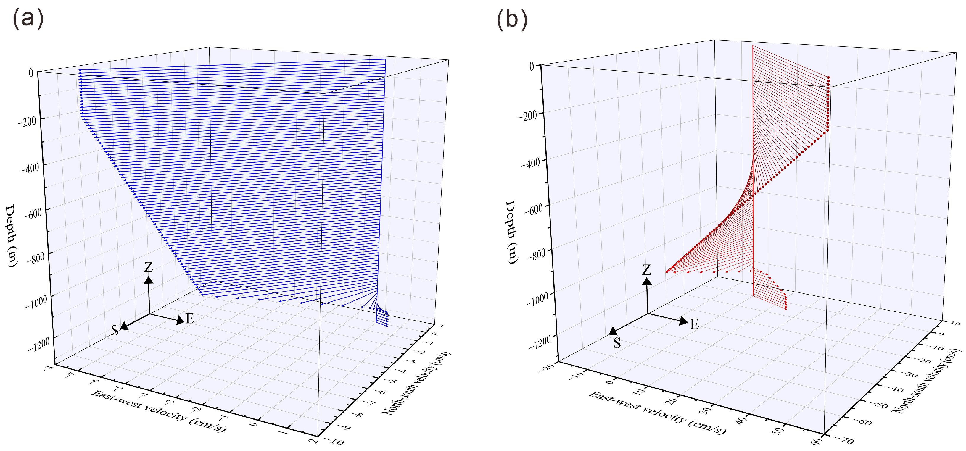
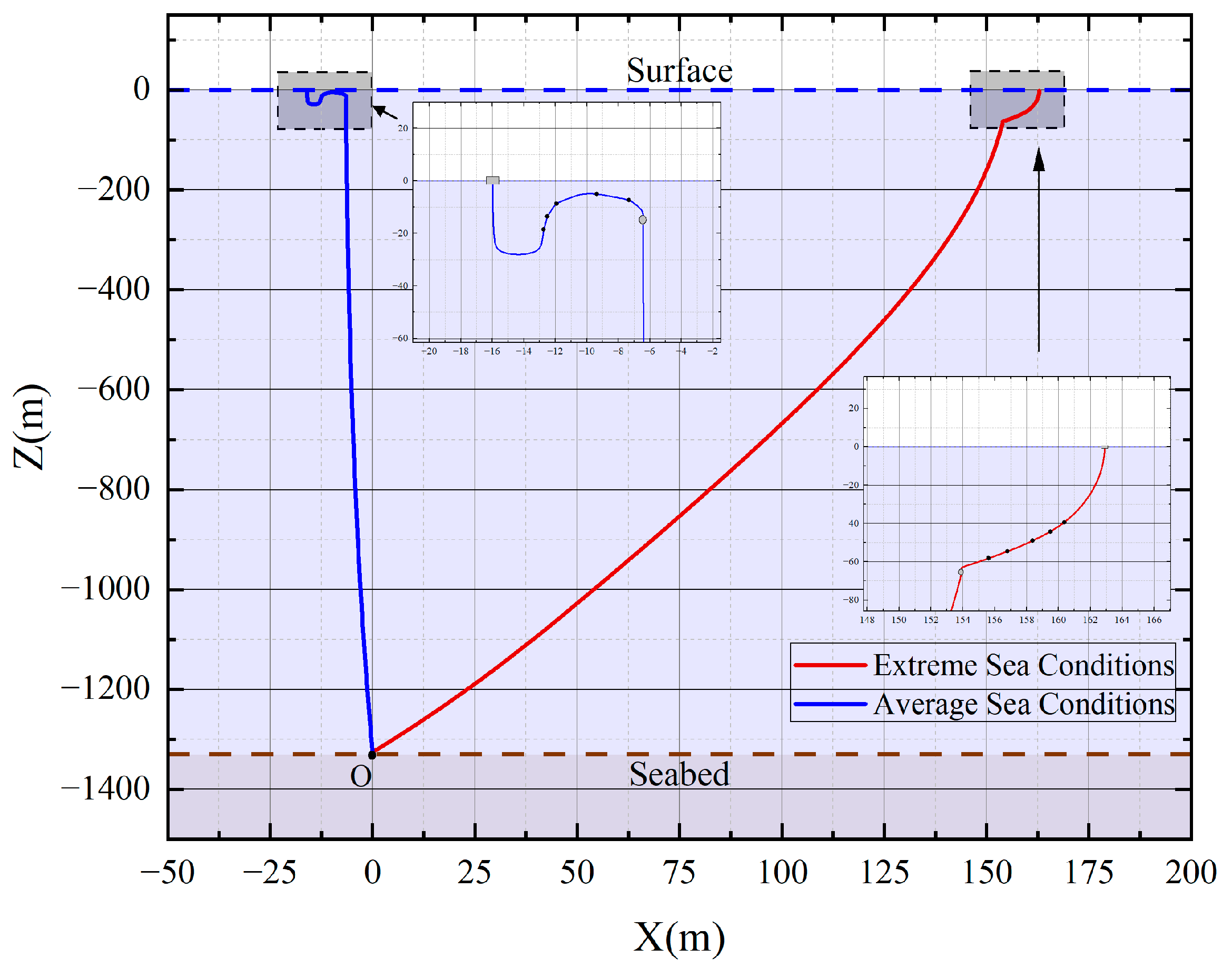
In the average sea condition as shown in Figure 4a, the current velocity ranges from 0.006 to 0.115 m/s, with 2 m wave height and 7 s wave period. The current direction is 231.02° counterclockwise with respect to the east. As the water depth increases, the current direction shifts toward the southeast, reaching a bottom direction of 340.75°. In the extreme sea conditions, the current speed ranges from 0.052 to 0.777 m/s, with 9.6 m wave height and 14.2 s wave period. The surface current direction is 313.21° counterclockwise with respect to the east. As depth increases, the current direction initially shifts toward the southwest, reaching a maximum deviation of 251.11°, and subsequently turns toward the southeast, with the bottom direction recorded at 341.22°, as illustrated in Figure 4b.

(3)

Modeling of the mooring structure

In the simulation, the water depth is 1330 m identical to the water depth of the realistic sea area for deployment of the system. Accordingly, based on deployment depth and manufacturing cost of cables, the total cable length is set to 1373 m.

To assess the influence of different mooring structures on the dynamic stability of the system, various mooring structures are proposed in the simulation. Figure 5a illustrates a straight-chain configuration simplified from the semi-taut moorings, where a single cable directly connects the buoy to the seabed node. Figure 5b presents the inverse-catenary mooring model incorporating a submersible buoy and a S-shaped configuration of the upper-armed EOM cable. The buoy is modeled as a cylinder with a diameter of 3 m, consisting of four vertically stacked segments with heights of 0.4 m, 0.4 m, 0.4 m, and 0.2 m, respectively, resulting in a total height of 1.4 m. The submersible buoy is represented by an ellipsoid model with a diameter of 2.5 m and a height of 3.0 m. The junction box is modeled as a rectangular prism with dimensions of 2.0 m × 2.0 m × 1.0 m. Detailed parameters of the above-mentioned mooring structure are listed in

Table 1. Configuration of model parameters.

Name of Components	Model Parameters	Applicable Configuration
Sea surface buoy	Cylinder Model, Six-Degree-of-Freedom (6D) Elements Diameter: φ 3.0 m Height: 1.4 m Weight: 4.5 t Total buoyancy: 98 kN	Straight-chain mooring; Inverse-catenary mooring.
Upper-armored cable	Diameter: φ 0.0473 m Weight: 5.1 kg/m Stiffness: Bending stiffness 0.2275 kN·m−2, Axial stiffness 112.3 × 103 kN, Torsional stiffness 3.25 kN·m−2 Minimum bending radius: 1 m Minimum breaking load: 1200 kN Safe working load: 300 kN Section length of upper cable: When Upper cable length = 15 m, the section length = 2-8-5 m (from top to bottom, the same below) When Upper cable length = 65 m, the section length = 2-18-12-24-2-2-5 m When Upper cable length = 115 m, the section length = 2-18-12-50-24-2-2-5 m When Upper cable length = 165 m, the section length = 2-18-12-50-50-24-2-2-5 m When Upper cable length = 215 m, the section length = 2-18-12-50-50-50-24-2-2-5 m	Inverse-catenary mooring.
Submersible buoy	Ellipsoid Model, Three-Dimensional (3D) Elements Diameter: φ 2.5 m Height: 3.0 m Volume: 5.5 m3 Weight: 1.2 t Total buoyancy: 53.9 kN	Inverse-catenary mooring.
Lower EOM cable	Diameter: φ 0.0364 m Weight: 2.2 kg/m Stiffness: Bending stiffness 0.1095 kN·m−2, Axial stiffness 51.99 × 103 kN, Torsional stiffness 0.593 kN·m−2 Minimum bending radius: 1 m Minimum breaking load: 530 kN Safe working load: 130 kN Section length of lower cable: (1) Straight-chain mooring model: Total cable length = 1373 m, the section length = 5-10-65-100 × 12-75-13-5 m (from top to bottom, the same below) (2) Inverse-catenary mooring model: When Upper cable length = 15 m, the section length = 5-10-50-100 × 12-75-13-5 m When Upper cable length = 65 m, the section length = 5-10-100 × 12-75-13-5 m When Upper cable length = 115 m, the section length = 5-10-50-100 × 11-75-13-5 m When Upper cable length = 165 m, the section length = 5-10-100 × 11-75-13-5 m When Upper cable length = 215 m, the section length = 5-10-50-100 × 10-75-13-5 m	Straight-chain mooring; Inverse-catenary mooring.
Seafloor junction box	Rectangular Prism, the Shape Model Size: 2.0 × 2.0 × 1.0 mm Weight: 4.0 t	Straight-chain mooring; Inverse-catenary mooring.
Bending reinforcements	Uniform Pipe Model Young’s modulus of material: 100 MPa Length: 2 m Inner Diameter: 0.049 m Outer Diameter: 0.05~0.15 m	Straight-chain mooring; Inverse-catenary mooring.

.

To accurately model the cable’s dynamic behavior in marine environments, JONSWAP wave spectrum (peak frequency 0.10097 Hz) is adopted in OrcaFlex. Hydrodynamic coefficients are configured as follows: drag coefficients (C_d) = 1.2 (transverse, x/y-direction), 0.008 (axial, z-direction); lift coefficient (C_l) = 0; added mass coefficients (C_a) = 1 (transverse, x/y-direction), 0 (axial, z-direction). Rayleigh damping is disabled, and the dynamic response is solved using implicit time-domain analysis for stable, efficient long-duration simulations.

In the simulation, the cable is discretized into multiple sections. Near the connection points between the cable and the buoy, submersible buoy, or junction box, lengths of sections are intentionally reduced to enable finer segmentation, thereby enhancing the accuracy of the simulation result. In contrast, section lengths in the mid-span region are increased to minimize the total number of sections, thus improving computational efficiency without compromising overall modeling fidelity. The complete cable segmentation scheme, the size of the cable, as well as the mechanical properties are shown in Table 1.

During the simulation, a time step of 0.1 s is adopted, and each operational condition is simulated for a total duration of 3600 s to guarantee that the system has reached the equilibrium state.

2.3. Offshore Experiment

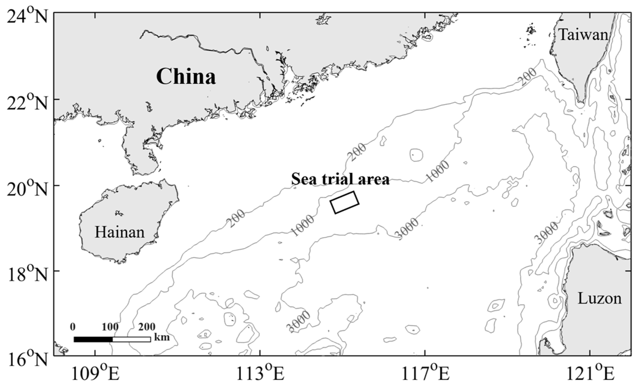
An offshore test for the monitoring system with the fabricated inverse-catenary mooring structure was conducted in the Shenhu area of the South China Sea (Figure 6). The water depth at the test site was 1330 m, with a seabed slope of 2°. The current velocity ranges from approximately 0.05 to 1.2 m/s, predominantly flowing in the southwest direction. The region is influenced by the northeast monsoon in winter, leading to a Level 5 sea condition according to wave classification standards. The average significant wave height was 2.0 m, while the maximum significant wave height could reach 9.5 m, corresponding to the Level 9 stormy sea condition. The sea trial was carried out on the “Marine Geological No. 2” vessel, operated by Guangzhou marine geological survey (GMGS).

During sea trial, the integrated monitoring system captures marine-atmospheric carbon cycling dynamics via multi-node sensors. Atmospheric CH₄ is measured by a buoy-mounted Aeris Ultra sensor, which has a range of 0.01~10,000 ppm, sensitivity < 1 ppb·s⁻¹, continuous operation, and 10 s sampling. For seawater parameters at buoy, submersible buoy and seafloor junction box, the following three sensors are used: Contros HydroC^TM CO₂ sensor (range 100~3000 ppm, resolution < 1 ppm), Contros HydroC^TM CH₄ sensor (range 1~40,000 μatm, resolution < 1 μatm), and METS CH₄ sensor (range 1~500 nmol·L⁻¹). All underwater gas sensors operate on a 1 h/12 h duty cycle with 5 s or 10 s sampling. Physical oceanographic parameters are collected by Sea-bird 16 plus V2 or 37 CTD and WHS-300 ADCP across all nodes, with a 30 min sampling interval. All sensors undergo annual calibration to ensure data reliability.

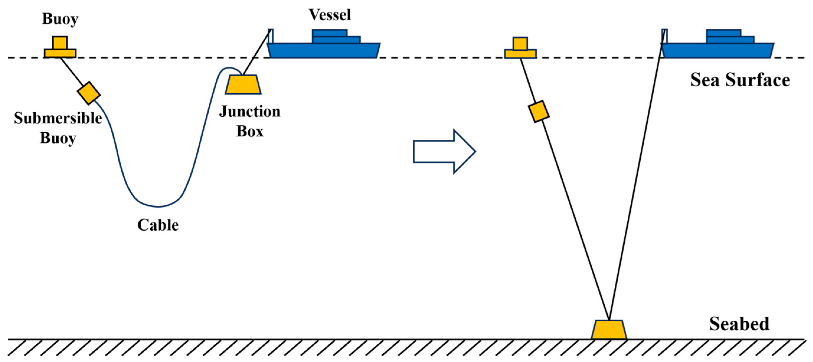
As shown in Figure 7, during the offshore deployment, the buoy, upper armored cable, submersible buoy, lower EOM cable, and the junction box were deployed sequentially from the mother ship equipped with the dynamic positioning (DP) system using the stern A-frame. The entire deployment process lasted approximately 10 h. Particular attention was given to ship speed control during the EOM cable deployment, as well as maintaining an appropriate distance between the vessel and the buoys.

3. Results and Discussion

3.1. Hydrodynamic Performance for Single-Point Mooring Cables

3.1.1. Effect of the Mooring Structure

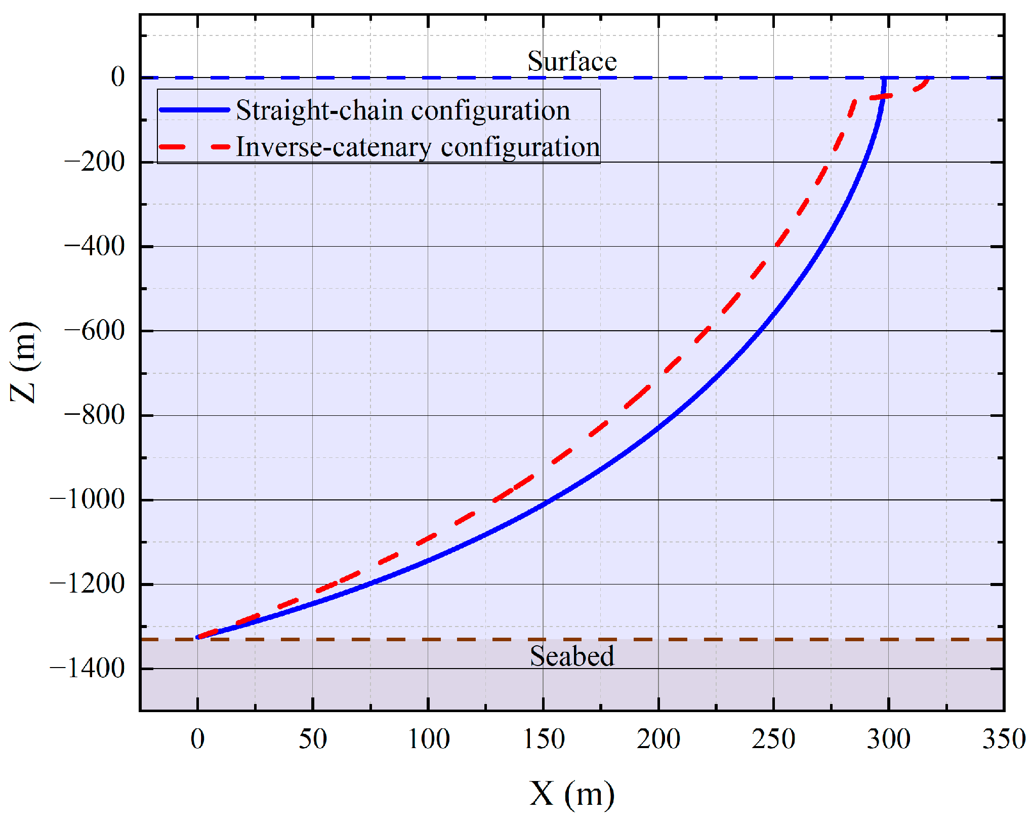
The effect of the mooring structure (Figure 5) on the hydrodynamic performance of the system is first investigated at the ideal sea condition, and the configuration formed when reaching the equilibrium state is shown in Figure 8. As introduced previously, the inverse-catenary mooring structure incorporates a submersible buoy near the sea surface, which divides the cable into upper and lower parts, forming a buffering structure above the submersible buoy. This structure prevents the impact of waves and surface current on the lower cable and the junction box on the seafloor. As shown clearly in Figure 8, obviously, displacement of the inverse-catenary mooring structure is smaller than the straight-chain mooring structure.

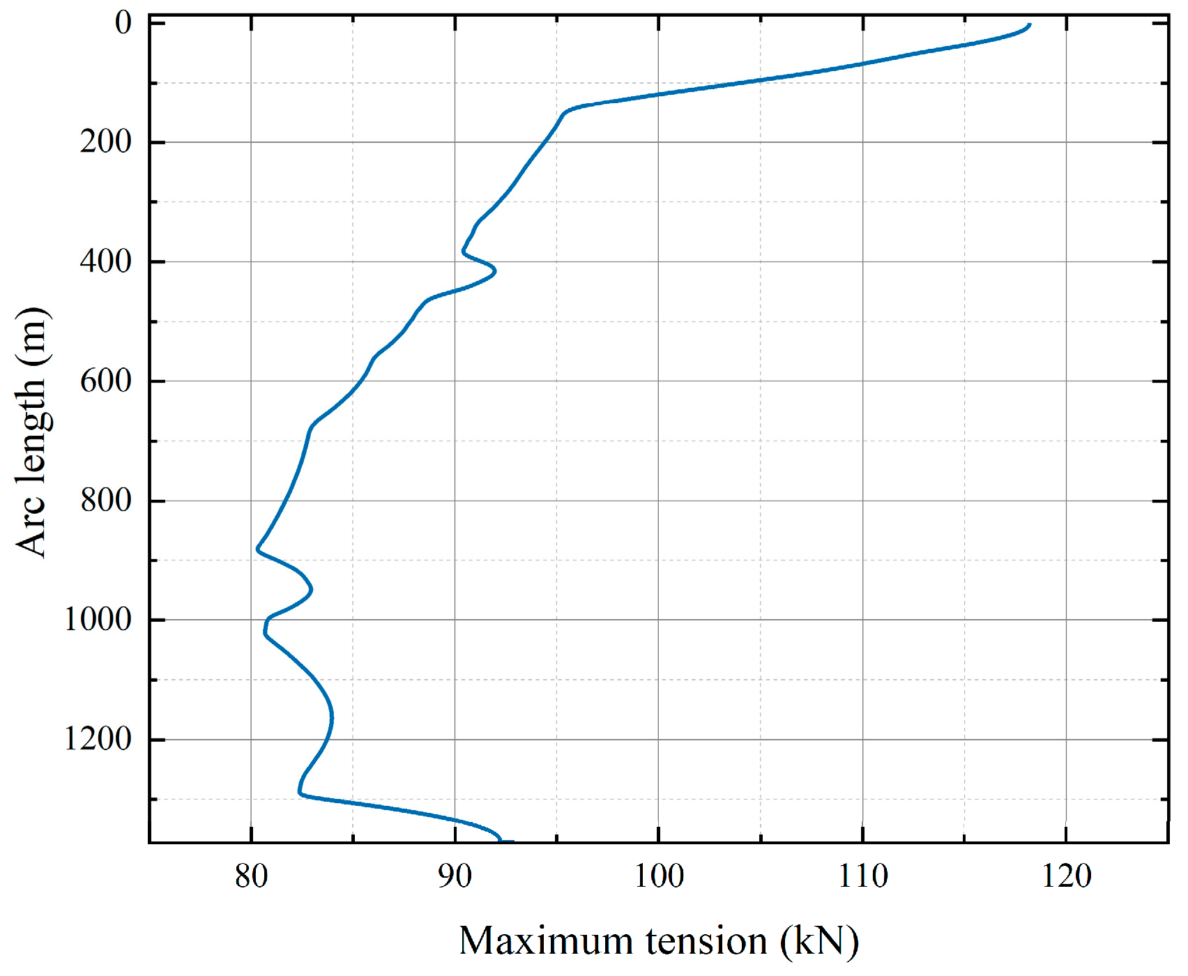
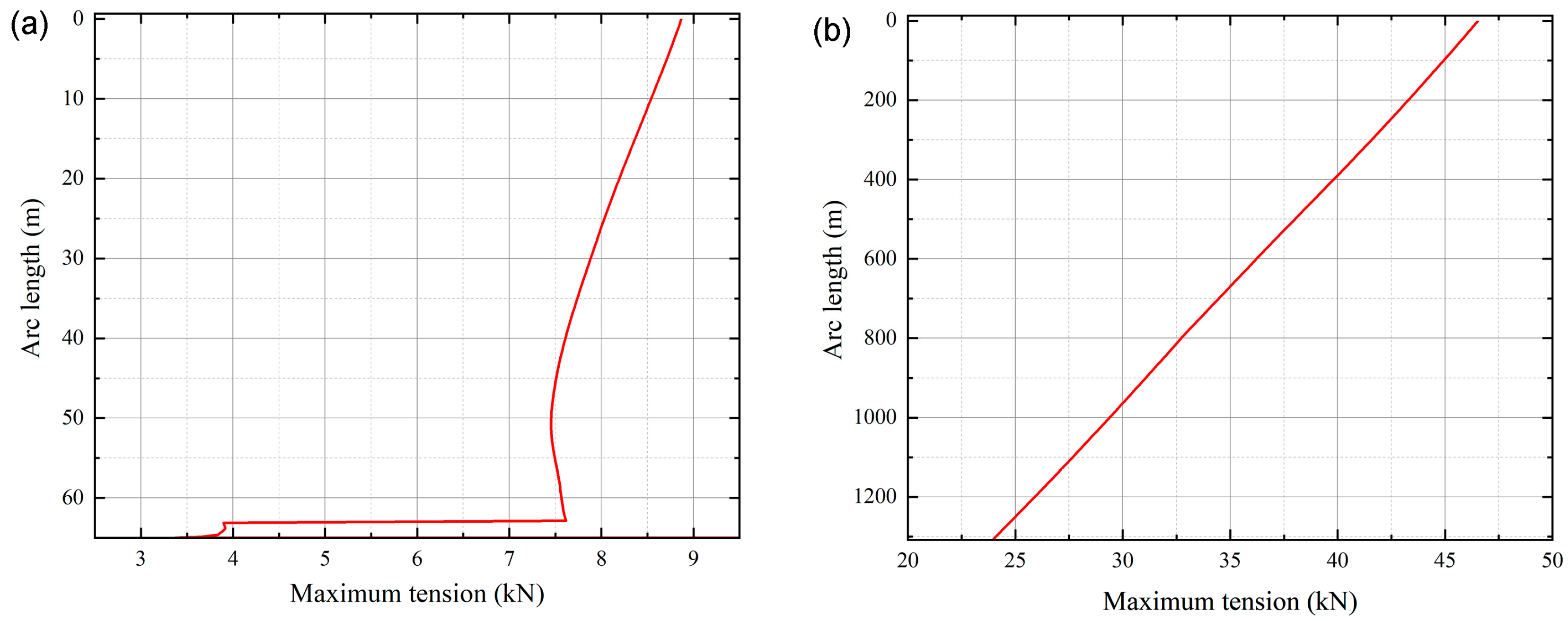
Figure 9 and Figure 10 show the maximum tension (defined as the temporal maximum tension on the cable at the equilibrium state) distribution along the cables for the two mooring structures. It is evident that the maximum tension is much lower for the inverse-catenary mooring structure compared to the straight-chain mooring structure (see

Table 2. Tension variations in cables under different mooring types.

Underwater Mooring Types and Connection Point Locations		Tension and Standard Deviation (KN)
		Max	Min	Mean	SD
Straight-Chain Mooing	between cable and buoy. A	118.166	−2.510	48.724	13.178
	between cable and junction box. B	92.830	−14.295	20.773	14.380
Segmented Inverse-Catenary Mooring	between upper cable and buoy. UA	8.868	0.320	3.475	0.851
	between upper cable and submersible buoy. UB	3.371	−0.326	0.169	0.323
	between lower cable and submersible buoy. LA	46.535	40.984	43.433	0.603
	between lower cable and junction box. LB	23.955	9.777	16.677	1.527

). The maximum tension in the straight-chain structure decreases nonlinearly with depth. Notably, a pronounced tension concentration occurs at the connection point located at the bottom of the buoy, with the maximum tension of 118.166 kN—substantially higher than 8.868 kN observed for inverse-catenary structure. Furthermore, the tension at the end of the buoy of the straight-chain mooring structure shows considerable fluctuation (see also Table 2), indicating strong influence from sea conditions and a tendency for the cable to experience the periodically tensile and compressive loads. On the other hand, with respect to the inverse-catenary mooring structure, the maximum tension at the end of the lower cable connecting to the junction box is 23.955 kN, which is lower than 92.830 kN in the straight-chain structure. These results indicate that the inverse-catenary structure effectively reduces the hydrodynamic tension by adopting the submersible buoy, reducing both the peak tension and tension fluctuations, especially at the ending of the cable connection the operation nodes. This is important for the long-term and reliable operation of the monitoring system. Therefore, the segmented inverse-catenary mooring structure is adopted for GOSMS.

3.1.2. Effect of the Length of the Upper Cable

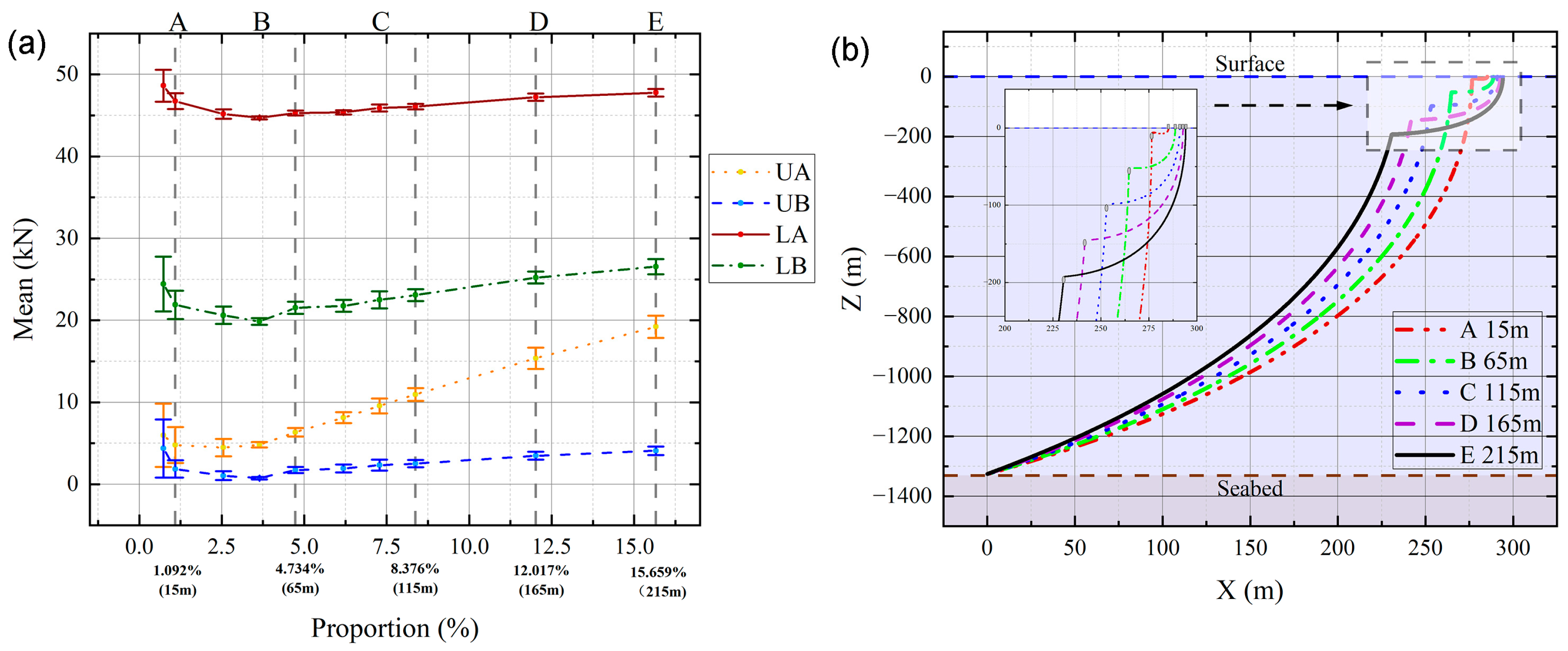
For the inverse-catenary mooring structure, the hydrodynamic performance with changing length of the upper cable is investigated by calculating the tension at key connection points of the cable at the ideal sea condition. The length of the upper cable varies from 10 m to 215 m and the lower segment changes accordingly, leading to the total cable length of 1373 m. To mitigate the impact of individual maximum tension extremes on simulation accuracy, the mean and standard deviation of the maximum tension values (top 1%) at each connection point were calculated. As shown in Figure 11a, with increasing length (or length proportion with respect to the total length of the cable) of the upper cable, change in tensions at the connection point of the buoy (UA), the upper and lower connection point of the submersible buoy (UB and LA), as well as the connection point on the junction box (LB) are similar, which first decrease to a minimum at the proportion of about 2.5%, followed by the continuous increasing. For UA with the length proportion above 2.5%, the maximum tension increases significantly, indicating that the dynamic load on the buoy rises with increasing upper cable length. In contrast, the maximum tension of UB and LA are relatively stable, which is due to the submersible buoy acting as a buffer that prevents the impact of the tension on the system below. The optimization objective is to minimize these maximum tension values, so the minimum at 2.5% represents the optimal stability condition.

From the above investigation, it is found that the upper cable with the length between 65 and 115 m (curves B and C in Figure 11b) is favorable, which has the minimum tension at all four connection points. It suppresses the vertical impact on UB if a lower upper cable is used. Also, it prevents additional tension on the nodes with longer cables and the corresponding cost since the upper cable is double-layer armored and thus has a much higher price compared to the lower cable.

3.1.3. Effect of Buoyancy of the Submersible Buoy

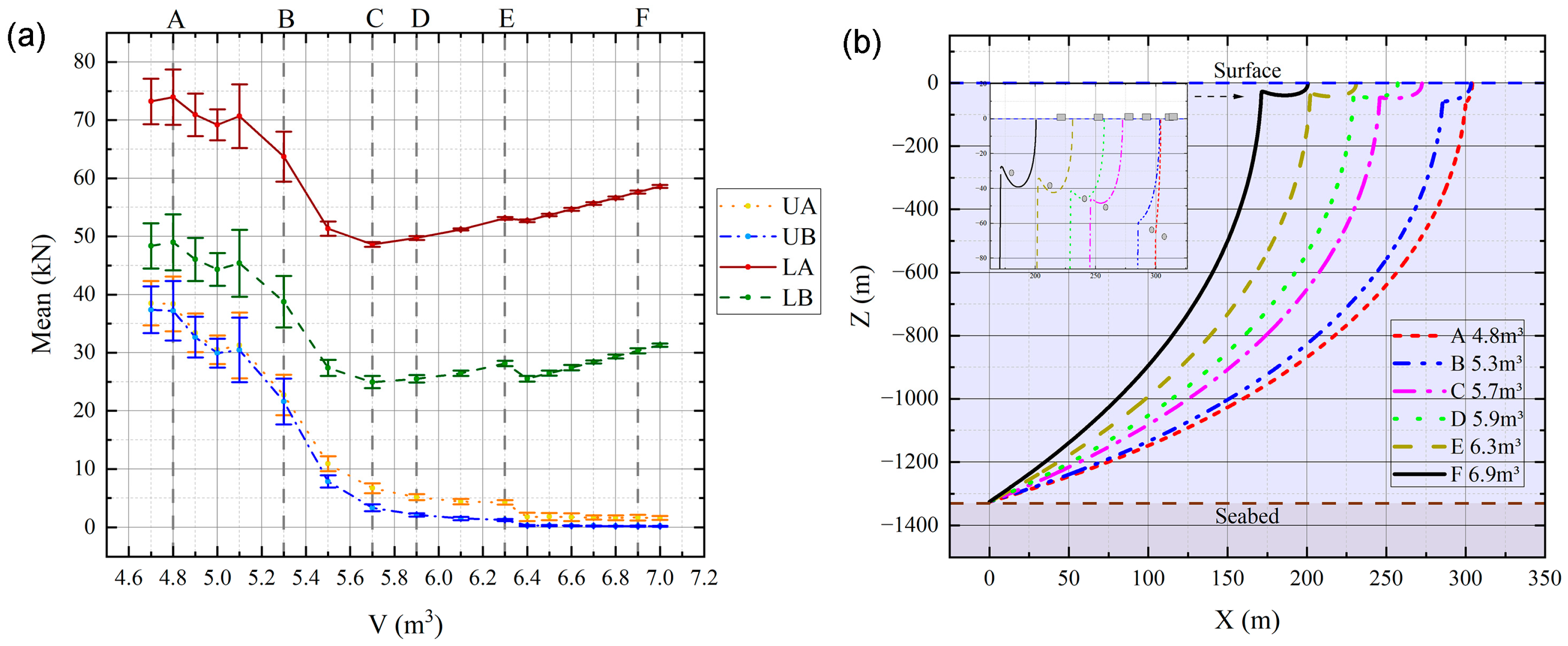
As discussed previously, in the inverse-catenary mooring structure, the submersible buoy buffers the impact from the current and wave near the sea surface. Its volume (i.e., buoyancy) directly affects the cable configuration and the hydrodynamic tension on the mooring structure. To investigate the effect of volume of the submersible buoy, length of the upper cable is kept at 65 m, and the length of the lower cable is 1308 m, with a total wet weight of 2878 kg. The volume of buoyancy material of the submersible buoy was selected within the range from 4.7 to 7.0 m³, and the corresponding buoyancy is from 47.4 to 70.3 kN. In this section, the mean and standard deviation of the top 1% of tension values at each connection point were also calculated.

As shown in Figure 12a, when the submersible buoy volume increases from 4.7 m³ to 7.0 m³, the tensions at both ends of the lower cable (LA and LB) exhibit an initial reduction followed by the increase. On the other hand, for the maximum tensions at UA and UB, it progressively decreases with increasing volume and eventually reaches a stable state. Notably, when the volume of the submersible buoy is between 5.5 and 5.9 m³, tensions for LA and LB reach minimum, meanwhile tensions for UA and UB are at low levels. Figure 12b shows the configuration of the mooring structure adopting the submersible buoy with various buoyancy. As the buoyancy increases, the submersible buoy is closer to the sea surface; meanwhile, the overall displacement of the mooring structure with the current reduced significantly indicating that the system could be more stable with variation in the current.

From the above investigation, it is considered that with the volume of the submersible buoy around 5.5 m³, a low level of cable tension could be achieved, which also has an acceptable cost compared to large ones.

3.2. Reliability Analyze for GOSMS

Based on the results of hydrodynamic simulations and parameter optimization, and considering practical manufacturing constraints and economic costs, we propose the optimized parameters of the mooring structure for the GOSMS and investigate the safety of the mooring system numerically at both average and extreme sea conditions. In the designed mooring system for GOSMS, the upper cable is 65 m long, with a multi-layer armored structure with a safe working load (SWL) of 300 kN and a minimum breaking load (MBL) of 1200 kN. It contains four electrical conductors and one pair of twisted wires. Five buoyancy blocks, each with 0.34 kN of buoyancy, are placed at the location of 34, 39, 44, 49, and 54 m along the cable away from the connection point of the buoy to maintain a S-shaped profile of the upper cable. The lower EOM cable has a length of 1308 m, for which a single-layer armored design with a safe working load of 130 kN and a minimum breaking load of 530 kN is employed. It integrates four electrical conductors, one pair of twisted wires, and two two-core optical fibers. The submersible buoy has a total volume of 5.5 m³, providing approximately 53.9 kN of total buoyancy.

Subsequently, the stability and safety performance of the proposed mooring configuration under average and extreme sea conditions is evaluated. Particular emphasis was placed on analyzing the maximum tension distribution on cable and at connection points, in order to verify whether the tension exceeds the SWL or MBL of the cables.

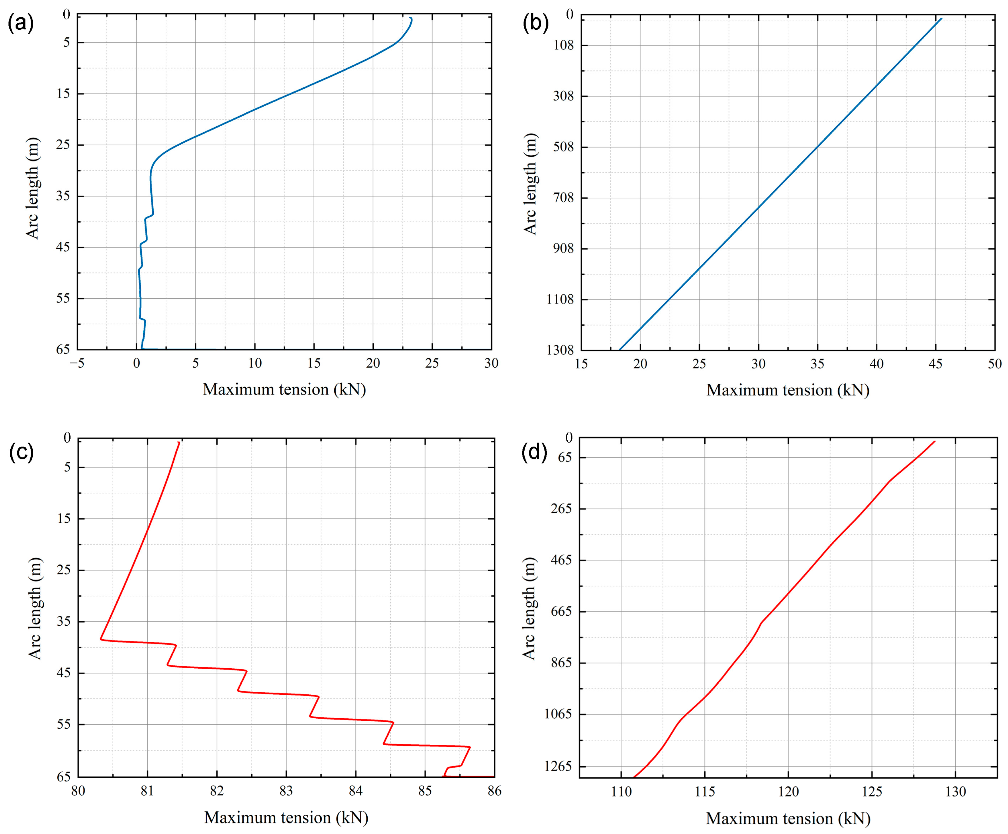
Figure 13a,b illustrate the variation in maximum tension along the upper and lower cable under average sea condition, while

Table 3. The variation in tension at different connections under various sea conditions.

Sea Conditions and Positions		Tension (KN)
		Max	Min	Mean	SD
Average Sea Condition	between upper cable and buoy	23.097	−0.394	1.344	0.825
	between upper cable and submersible buoy	0.418	−0.312	−0.025	0.089
	between lower cable and submersible buoy	45.498	40.995	43.289	0.656
	between lower cable and junction box	18.195	13.279	15.632	0.689
Extreme Sea Condition	between upper cable and buoy	81.438	−4.856	14.678	15.758
	between upper cable and submersible buoy	84.965	−1.259	13.087	15.627
	between lower cable and submersible buoy	128.765	24.214	56.323	15.636
	between lower cable and junction box	110.715	−11.024	29.749	16.886

presents the changes in maximum, minimum, average tension, and standard deviation at each connection point along the cables. The maximum tension distribution in the upper cable decreases non-linearly with length and eventually reaches a stable state. The peak tension occurs at the connection point between cable and buoy, with a value of 23.097 kN. By contrast, the maximum tension in the lower cable follows a linear decreasing trend along its length, with the maximum of 45.498 kN at the connection point below the submersible buoy. Overall, under average sea conditions, the underwater cable system forms a gentle S-shaped configuration, with a relatively uniform tension distribution (Figure 14).

The maximum tension distribution on the upper and lower cable under extreme sea conditions are shown in Figure 13c,d. The maximum tension in the upper cable first decreases and then increases in a stepwise form as shown in Figure 13c due to the presence of buoyancy blocks, with the turning point at about 38 m. The maximum tension peaks near the submersible buoy at over 85.5 kN. On the other hand, the tension on the lower cable maintains a linear decreasing trend similar to that observed under average sea condition, decreasing from 128.765 kN at the end of the submersible buoy to 110.715 kN at the connection point of the junction box. As shown in Figure 14, the cable system drifts significantly with the current under the extreme sea condition, causing sharp tension increases in the upper cable and also higher tension levels in the lower cable compared to the average sea condition.

In summary, from the numerical simulation, we find that with the optimized design of the mooring system for GOSMS,

(1)

The maximum tension of the upper cable is lower than 86 kN in all sea conditions, well below its SWL of 300 kN and MBL of 1200 kN. Due to the complex hydrological conditions in the surface layer, a multi-layer armoring design is adopted for the upper cable, which provides sufficient safety margin and reduces torsional fatigue.

(2)

Under the extreme sea condition, the maximum tension in the lower cable with a single-layer armoring design reaches 128.765 kN, which is well below its SWL (130 kN) and MBL (300 kN). This gives a sufficient safety margin ensuring the lower cable’s suitability for deep-sea and long-term deployment.

3.3. Offshore Deployment of GOSMS

The development of the fabricated GOSMS based on the optimized designed inverse-catenary mooring structure is successfully deployment to the NGH zone in the “Shenhu” area of the South China Sea at the sea-depth of 1330 m, as shown in Figure 6 and Figure 15. The system transmits the data to the stations on land twice a day, enabling continuous monitoring of the system’s status, as well as the environment of multiple layers—including the seabed boundary layer, water column, and sea-air interface.

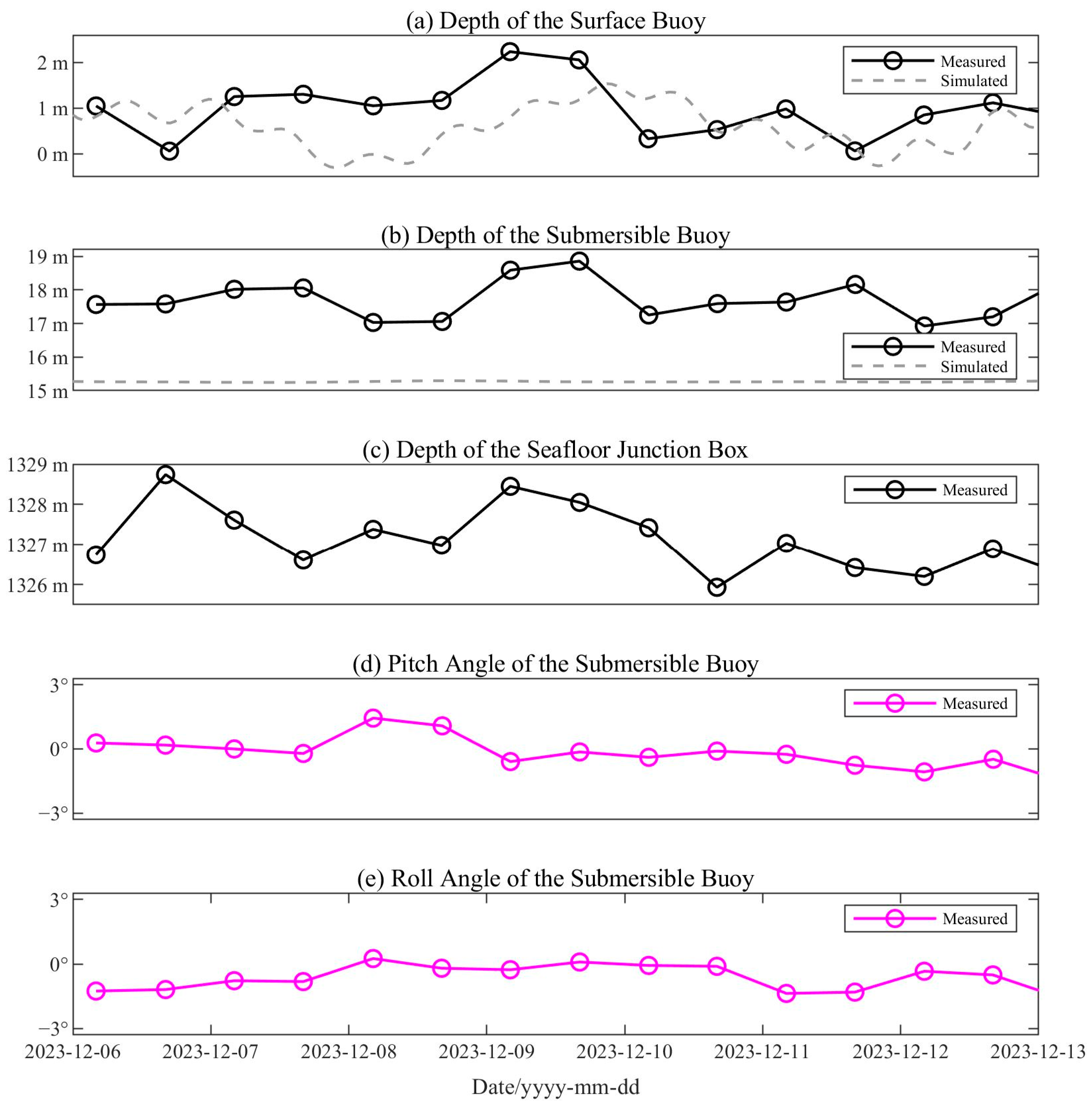
The stability of the mooring structure of GOSMS during the offshore deployment is assessed by the displacement of buoy, as well as the pitch and roll motion of the submersible buoy. As shown in Figure 16a, the measured water depth of the buoy ranges from 0.33 to 2.24 m. This is similar to the displacement of the junction box that is supposed to be static on the seabed (see Figure 16c), the depth of which varies between 1325.93 and 1328.74 m. The fluctuation of the water depth is considered to be caused by the tidal evolution between −0.60 and 0.65 m, with tidal data derived from the Tidal Model Driver (TMD) toolkit developed by the University of Oregon [46]. This indicates that the buoy maintained a stable attitude, which is not sensitive to the wind, waves, and the surface current. Figure 16b shows that the water depth for the submersible buoy, the fluctuation amplitude is around 1.9 m, which is larger than the simulation (within 0.1 m) at the average sea condition considering also the tidal effect. Furthermore, the attitude variation in submersible buoy is measured by underwater inclination sensor, as shown in Figure 16d,e, which present the pitch and roll angle changes observed during the sea trial. The pitch angle ranged from −1.48° to 1.44°, and the roll angle from −1.37° to 0.09°, both within a narrow range of less than 3° and without abrupt changes. This suggests that the submersible buoy remained stable during operation, experiencing minimal disturbance from wave action or ocean currents, and no significant tilting or rolling occurred. The motion of the mooring system measured during the deployment shows that the system is stable for reliable and continuous environment monitoring.

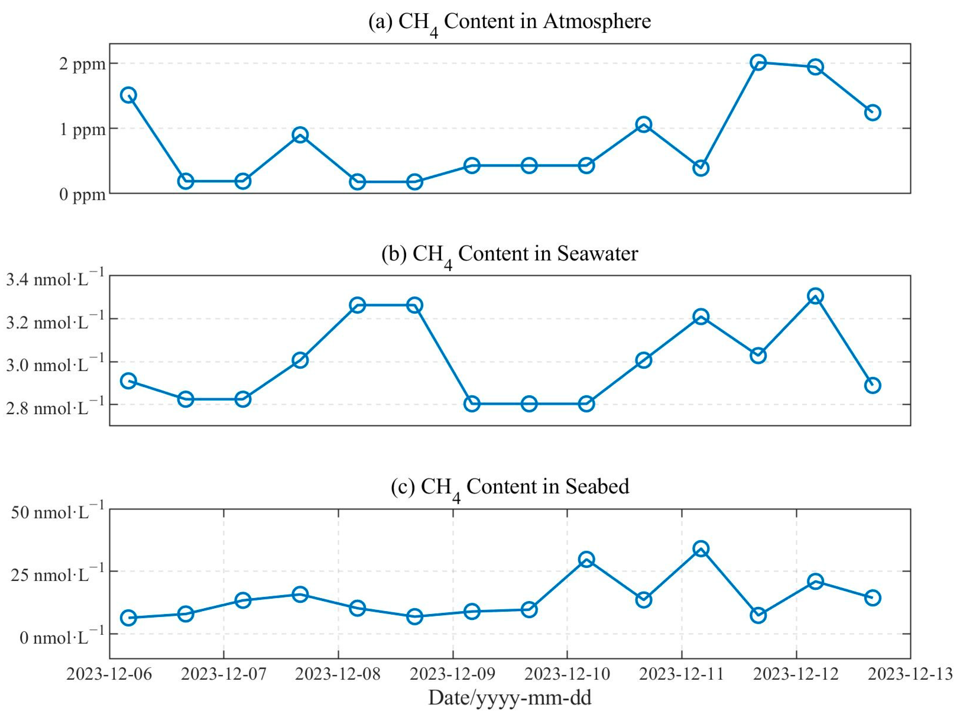
During the offshore test of GOSMS at the NGH zone, variations in methane concentration at different water layers are successfully measured through sensors installed at surface and submersible buoys as well as the junction box on the seabed, as shown in Figure 17. The methane content ranges from 6.42 to 34.08 nmol·L⁻¹ at the seabed boundary layer, from 2.80 to 3.26 nmol·L⁻¹ at the top layer of sea water, and from 0.20 to 2.01 ppm in the air above the sea surface. The result is consistent with previously collected environmental baseline data from this region [47,48,49,50]. This indicates that GOSMS developed is reliable.

3.4. Advantages and Limitations of GOSMS

As the mooring configurations, deployment water depths, and application scenarios of different ocean observation systems differ substantially, and there is no similar deep-water observation system in the northern South China Sea, it is currently difficult to provide a quantitative evaluation of the optimization effect of the underwater mooring structure in this paper. However, compared with other observation systems, the GOSMS is based on an optimized segmented inverse-catenary mooring configuration, achieving an overall optimum in terms of minimum tension, cost constraints and deployment flexibility (see

Table 4. Comparison between GOSMS and other existing technologies and equipment.

Items	GUMBY System	Coastal Surface Moorings of OOI	MOOS	OCB System	MBOSBC	GOSMS, This Paper
Underwater mooring configuration	Semi-taut	Semi-taut	Inverse-catenary	Inverse-catenary	Inverse-catenary	An optimized segmented inverse-catenary
Deployment depth	144 m	450 m	Designed for 4000 m, deployed at 1875 m	Designed for 3000 m, deployed at 1000~2800 m	20 m	1330 m
Monitoring layer	Underwater (at a depth of 20~35 m)	Sea surface, near surface (at a depth of 7 m), seabed	Sea surface, seabed	Sea surface, seabed	Sea surface, seabed	Sea-air interface, euphotic zone, seabed
Main monitoring purpose	Movement of whales	Meteorological conditions, oceanographic properties, and sea-air interactions	Marine meteorology, ocean physical processes, and water quality	Seafloor pressure; the impact of tsunamis caused by submarine earthquakes	Marine meteorology, ocean physical processes, and water quality	Stereoscopic monitoring of methane leakage in NGH areas
Data transmission method	Electrical cables	Electrical cables	Optical fibers, electrical cables	Optical fibers, electrical cables	Optical fibers, electrical cables	Optical fibers, electrical cables, and acoustic transmission
Power supply method	Alkaline battery pack	Solar and wind power	Solar and wind power	Diesel generator power	Solar and wind power	Solar power

). The application water depth of this system reaches 1330 m, which is comparable to that of MOOS and OCB systems. In terms of monitoring layers, GOSMS has added the monitoring of environmental parameters such as methane content in the euphotic zone, improving the stereoscopic monitoring ability of methane leakage. In addition, for data communication, dual-insurance transmission via EOM cables (integrating optical fibers and electrical conductors) is employed, with acoustic communication serving as a backup to enhance data transmission redundancy.

Although the first sea trial of GOSMS was successful, there are still some limitations and problems during the system design, simulation, and offshore deployment. First, during the simulation, this study mainly focused on the influence of different mooring configurations on the system’s stability. Parameters such as the total length of the cables, the length of the upper cable, and the buoyancy of the submersible buoy were fixed, and no sensitivity analysis of key parameters was carried out. The simulation results may be slightly affected by the uncertainty of the parameters. Second, since the system’s first sea trial lasted about 4 months, the fatigue damage of the cables under long-term mooring was not considered. Finally, during the sea trial, due to the incorrect estimation of the lowering speed of the junction box, the overall deployment time was extended from the planned 6 h to 10 h, which also greatly increased the risk of damage to the EOM cable. Next, researchers will conduct sensitivity analysis of key parameters to quantify the impact on simulation accuracy, supplement the research on the fatigue damage and fatigue identification of the mooring cables under long-term mooring situation, and further optimize the system deployment and recovery processes.

4. Conclusions

The GOSMS for multi-water-layer environmental monitoring in the NGH zone at the water depth of 1330 m is developed based on an optimized segmented inverse-catenary mooring configuration composed with buoy-upper cable-submersible buoy-lower cable-seafloor junction box, from the top to the bottom. Through a detailed numerical simulation, it is found that by incorporating the submersible buoy in the mooring structure, deformation of the cable configuration and tension are effectively suppressed especially at the part below the submersible buoy. Consequently, the overall stability of the system was markedly improved. Moreover, the length ratio between the upper and lower cables, as well as the buoyancy volume of the submersible buoy, are identified as critical parameters affecting the stability of the underwater mooring cables. Based on the numerical simulation, the GOSMS with improved mooring structure is successfully deployed and tested at a depth of 1330 m in the Shenhu NGH area of the northern South China Sea, showing satisfying stability in the harsh winter sea condition. Furthermore, the system also achieved reliable in situ monitoring and real-time transmission of environmental parameters in multi-water layer including the evolution of methane concentration during the offshore test. Future optimizations including enhanced cable mooring reliability and underwater data interfaces will improve system’s versatility and scalability, enabling integration with regional marine observation networks and expanding applications in deep-sea exploration and carbon sequestration monitoring.