Article

Channel Confinement Drives Unidirectional Migration: Coupling of Flow Structure and Sedimentary Evolution in Combined Turbidity–Bottom Current Flows

1
Hubei Key Laboratory of Marine Geological Resources, China University of Geosciences (Wuhan), Wuhan 430074, China
2
College of Marine Science and Technology, China University of Geosciences (Wuhan), Wuhan 430074, China
3
Research Institute for Intelligent Earth Systems, Marine Science and Technology College, Zhejiang Ocean University, Zhoushan 316022, China
4
Petro China Hangzhou Research Institute of Petroleum Geology, Hangzhou 310023, China
*
Author to whom correspondence should be addressed.
These authors contributed equally to this work and share first authorship.
J. Mar. Sci. Eng. 2026, 14(2), 152; https://doi.org/10.3390/jmse14020152
Submission received: 19 December 2025 / Revised: 6 January 2026 / Accepted: 7 January 2026 / Published: 11 January 2026
(This article belongs to the Section Geological Oceanography)

Abstract

Along-slope bottom currents and down-slope (gravity-driven) turbidity currents coexist in the ocean and interact during their flow processes. The interaction between turbidity currents and bottom currents plays a crucial role in determining the lateral stacking of sediments and the direction of channel migration. Currently, there is ongoing debate regarding the migration direction, with two primary contrasting views: upstream migration versus downstream migration relative to the bottom current. However, due to the challenges in directly observing unidirectionally migrating channels in nature, the sedimentary hydrodynamics and underlying flow mechanisms remain poorly understood. In this study, we employ numerical simulations to systematically analyze the internal flow characteristics and depositional patterns within channels subjected to varying degrees of confinement. Our results demonstrate that variations in channel confinement influence the intensity of the interaction and the nature of the secondary flow, ultimately determining the spatial distribution of sediments. As confinement decreases, the migration pattern of a channel changes from negligible migration to migration in the downstream direction of the bottom current. Subsequently, it changes to migration in the upstream direction of the bottom current. This research provides a novel theoretical perspective for understanding the diametrically opposite migration directions of unidirectionally migrating channels and insights into the turbidity–bottom current interaction processes and the evolutionary mechanisms of deep-sea depositional geomorphology.

1. Introduction

Along continental margins worldwide, interactions between bottom currents (along-slope flows) and turbidity currents (down-slope flows) are widespread and have a significant influence on sediment transport from source to sink. In recent years, the impact of turbidity–bottom current interactions on the sedimentary evolution of submarine channels has garnered increasing attention [1,2,3]. Since Rasmussen (1994) [4] first reported the lateral migration of turbidity current channels influenced by bottom currents offshore Gabon, West Africa, similar phenomena have been observed and studied in various marine regions. These include the Nova Scotia margin in North America [5,6], the Lower Congo Basin offshore West Africa [7], the South China Sea [8,9,10], the Mozambique margin offshore East Africa [11,12], the Antarctic Peninsula [13,14], and the Argentine continental margin offshore South America [15], among others. Gong et al. (2013) [10] defined the term “unidirectionally migrating channels” to describe these channels.
However, according the present publications, the migration direction of these unidirectionally migrating channels follows two contrasting patterns: one migrates downstream relative to the bottom current [7,8,10,15,16], while the other migrates upstream [5,6,11,12,17]. Studies on downstream migration suggest that it may be related to the development of a counter-flow secondary circulation within the channel, which transport near-bed sediment upstream [7]. Additionally, Kelvin-Helmholtz billows and bores induced by turbidity–bottom current interaction can cause erosion on the downstream side of the bottom current (wave front) and deposition on the upstream side (wave tail) [18]. Conversely, upstream migration mechanisms may involve the Lee Wave theory [5] or the formation of overbank drift deposits by fine-grained sediments on the downstream side of the bottom current, which could promote upstream channel migration [12]. Furthermore, Rasmussen et al. (2003) [19] proposed that variations in migration direction are controlled by the relative strengths of the turbidity current and the bottom current, where a stronger bottom current favors downstream migration. Chen et al. (2020) [11] suggested that helical secondary flows in sinuous channels could be enhanced or counteracted by the bottom current, thereby influencing the migration direction. Although these studies provide potential mechanisms from different perspectives, a unified theoretical framework capable of explaining the contrasting migration directions remains lacking.
Based on a systematic statistical analysis of the width-to-depth ratios of unidirectionally migrating channels influenced by turbidity–bottom current interactions worldwide (Table 1), a series of channels with extremely small width-to-depth ratios (averaging approximately 1.57) developed on the Pacific margin of the Antarctic Peninsula exhibiting no distinct migration trend [3,14]. In the Pearl River Mouth Basin, the Mauritania Basin, and the Lower Congo Basin, unidirectionally migrating channels with moderate width-to-depth ratios (approximately 13.43–24.44) consistently migrate downstream relative to the bottom current [7,10,16] (Table 1). In contrast, channels along the Tanzanian margin, Mozambique margin, and Nova Scotia margin, which have relatively large width-to-depth ratios (approximately 29.17–38.89), show a trend of upstream migration relative to the bottom current [5,12,20] (Table 1). Notably, offshore southeast Greenland, both migration directions coexist [19]. Specifically, early-stage channels migrated upstream, while late-stage channels migrated downstream, with the channel morphology transitioning from weakly confined in the early stage to strongly confined in the later stages (See Figure 9 by Rasmussen et al., 2003 [19], absence of vertical and horizontal scale information, the width-to-depth ratio cannot be calculated). Therefore, the channel width-to-depth ratio appears to be a key parameter influencing the migration direction of channels under turbidity–bottom current interaction.
During channel evolution, variations in geometric parameters provide feedback to the internal flow behavior which in turn influences subsequent hydrodynamic structures and depositional processes, forming morphodynamic feedback [21,22,23,24]. Adema et al. (2025a) [23] investigated the response of three channels with different depths to bottom current, finding that the secondary flow on the downstream side of the bottom current intensified as channel depth increased. In their study, the width-to-depth ratio corresponds to the channel confinement; variations in channel confinement affect the flow structure, thereby influencing sedimentation.
Previous studies have proposed that channel confinement is primarily shaped by the combined effects of flow structure and sediment deposition [25]. However, due to the inherent complexity of natural environments and limitations in observational techniques, directly observing the internal flow characteristics and modern sedimentary features of submarine channels is challenging. Furthermore, due to the potential interference of complex real-world topography on flow structure, it is often difficult in studies of actual seafloor settings to pinpoint exactly which factor influences the lateral migration of submarine channels. Consequently, much of the research relies on numerical simulations or flume experiments [23,24,25,26,27,28]. Among these approaches, numerical simulation offers significant advantages in visualizing complete flow field structures and adjusting parameters, combining both intuitive understanding and cost-effectiveness. This method has proven highly effective in elucidating channel evolution mechanisms [26,29,30,31,32].
Building upon this research background, the present study developed a series of channel models with varying width-to-depth ratios. This study focuses exclusively on the effect of a single variable—channel confinement (channel width-to-depth ratio)—on lateral channel migration, while treating all other factors as constants to minimize interference with the results. By comparing flow characteristics within channels with different width-to-depth ratios, this study investigates the migration mechanisms of channels with varying degrees of confinement under the combined control of turbidity and bottom currents from a hydrodynamic perspective. The results demonstrate that the channel width-to-depth ratio plays a significant role in regulating the intensity of turbidity–bottom current interaction, the internal secondary flow structure, and the spatial distribution of sediment, thus governing the direction of channel migration. From a morphodynamic perspective, the study reveals the controlling role of channel confinement in migration behavior during turbidity–bottom current interaction. It provides a unified theoretical framework for understanding the divergent migration mechanisms of unidirectionally migrating channels across different geological settings and offers a numerical simulation-based foundation for deepening the understanding of deep-sea sedimentary system evolution.

2. Method

2.1. Flow Parameterization

This study systematically employs dimensionless parameters, such as the Froude number (Fr) and Reynolds number (Re), alongside physical quantities including flow thickness, shear velocity, cross-stream velocity, particle volumetric concentration, and density, to analyze the influence of the width-to-depth ratio on the flow behavior of combined turbidity–bottom current flows.
Dimensionless numbers are essential for characterizing the fundamental properties of the flow and its sedimentary response [33,34,35,36,37]. Among these, the Reynolds number (Re) and the Froude number (Fr) are commonly used to describe the intrinsic properties of the flow itself [31,36,37]. This study employs these two key parameters to investigate the effect of the width-to-depth ratio on the characteristics of combined flow.
The Reynolds number shows the comparative significance of inertia forces versus viscous forces in the fluid. A higher value signifies a greater turbulent nature of the flow. It is calculated using the following formula:
R e = ρ U h μ
where U is the depth-averaged flow velocity, h is the depth-averaged height of the fluid, U = 0 | u | 2 d z 0 | u | d z , h = ( 0 | u | d z ) 2 0 | u | 2 d z , with | u | = ( u 2 + v 2 ) [33]; ρ is the fluid density; and μ is the dynamic viscosity of the fluid.
The Froude number quantifies the relative strength of inertial forces to gravitational forces. When Fr > 1, the flow is supercritical, while r < 1 indicates subcritical flow. With Fr = 1 as the threshold, subcritical flow tends to favor net deposition, whereas supercritical flow is more conducive to net suspension [38,39]. The calculation formula for the Froude number is:
F r = U g h
The Froude number is given by g = C g ( ρ ρ a ) ρ a , where ρ a is the ambient fluid density, g is the acceleration due to gravity, and C = 0 c | u | d z U h , with c representing sediment concentration.
The fluid thickness is defined, following Miramontes et al. (2020) [28], as the height at which the velocity reaches half of its maximum value. The shear velocity ( u * ) quantifies the turbulent shear at the flow bottom and is closely related to the bed shear stress. It is a crucial parameter for assessing the sediment transport capacity of the flow and governing the behavior of turbidity currents [39,40,41]. The formula for calculation shear velocity is:
u * = u m κ ( l n ( h m 0.1 d 90 ) ) 1
where u m is the maximum velocity; h m is the height at which the maximum velocity occurs; κ is the von Karman constant; and d 90 is the grain size corresponding to the 90% cumulative percentage in the grain-size distribution of the turbidity current.

2.2. Governing Equations

Utilizing the ANSYS-CFD (2022.1) numerical simulation platform and an Eulerian multiphase model based on the finite volume method, we solved the mass and momentum conservation equations for seawater and sediment particles [26,42,43,44]. Together, the mass conservation equation and the momentum conservation equation collectively form the fundamental equations of the Reynolds-Averaged Navier–Stokes (RANS) equations.
Mass balance equation:
t + x ρ u + y ρ v + z ρ w = 0
Momentum balance equation:
t + u x + v y + w z = 1 ρ p x + G x + f x
t + u x + v y + w z = 1 ρ p y + G y + f y
t + u x + v y + w z = 1 ρ p z + G z + f z
where ρ is the local mixture density. u ,   v ,   and   w represent the velocity components in the x-, y-, and z-directions, respectively. f x , f y , and f z are viscous accelerations in the x-, y-, and z-directions, and G x , G y , and G z are the body accelerations in the corresponding directions.
This study employs an Eulerian multiphase flow numerical model, which focuses on fixed spatial points and solves a set of momentum and continuity equations for each phase independently. For granular flow, the characteristics are derived using kinetic theory. The equations governing multiphase flows are presented here for the general case of an n -phase flow. The volume of phase q , denoted by V q , is described as follows [26,44,45]:
V q = V a q d V
where a q is the volume fraction of phase q , and q = 1 n a q = 1. The effective density of phase q , ρ ^ q , is given by:
ρ ^ q = a q ρ q
where ρ q represents the physical density of phase q .
For the specific phase q , Equations (4)–(7) can be modified to Equations (10) and (11) in the Eulerian multiphase model:
t a q ρ q + · a q ρ q v q = p = 1 n ( m ˙ p q m ˙ q p ˙ )
where v q represents the velocity of phase q, m ˙ p q describes the mass transfer from phase p to phase q , and m ˙ q p describes the mass transfer from phase q to phase p
t a q ρ q v q + · a q ρ q v q v q = a q P + · τ ̿ q + a q ρ q g + p = 1 n R p q ( m ˙ p q v p q m ˙ q p v q p ) + { F q + F w l , q + F l i f t , q + F v m , q + F t d , q }
Here P represents the pressure for all phases; g denotes the gravitational acceleration; τ ̿ q indicates the stress tensor for the q t h phase; K p q represents the interphase momentum exchange coefficient; v q and v p represent the phase-weighted velocities for the q t h and p t h phases, respectively; v p q is the interphase velocity, defined as follows. If m ˙ p q > 0 (meaning that mass from phase p is being transferred to phase q ), then v p q = v p ; if m ˙ p q < 0 (meaning that mass from phase q is being transferred to phase p ), then v p q = v q . Similarly, if m ˙ q p > 0, then v q p = v q ; if m ˙ q p < 0, then v q p = v p ; n is the total number of phases; F q denotes an external body force acting on the q t h phase; F w l , q represents a wall lubrication force; F l i f t , q represents a lift force; F v m , q represents a virtual mass force; and F t d , q represents a turbulent dispersion force. The stress tensor τ ̿ q is defined by
τ ̿ q = a q μ q v q + μ q T + a q λ q 2 3 μ q · v q I ̿
where λ q represents the bulk viscosity of the q t h phase; μ q represents the shear viscosity of the q t h phase; and I ̿ represents the identity tensor.
Equation (11) must be closed by an appropriate expression for the interphase force R p q . This force depends on friction, pressure, adhesion, and other effects, and is subject to the following constraints: R p q = R q p , R q q = 0 .
Fluent uses the following form for the simple interaction term:
p = 1 n R p q = p = 1 n K p q ( v p v q )
where K p q is the interface momentum exchange coefficient, K p q = ρ p f 6 τ p d p A i . A i is interface area; f is resistance function; τ p is the particle relaxation time, defined as τ p = ρ p d p 2 18 μ p , here, d p is droplet diameter of phase p . v p and v q represent the phase velocities, respectively.
Turbulence models can be applied across the full-scale, particularly in complex terrain with high Reynolds numbers, providing critical insights into the development of submarine channels and sedimentation–erosion processes [27,29,30,31,32,43]. This study employs the k-ε turbulence model and utilizes a mathematical technique known as Renormalization Group (RNG) for derivation. The turbulent kinetic energy (k) and its dissipation rate (ε) are derived from the following transport equations:
t ρ k + x i ρ κ u i = x i a k μ t k x j + G k + G b ρ ε Y M
t ρ ε + x i ρ ε u i = x j a ε μ t ε x j + C 1 ε ε k G k + C 3 ε G b C 2 ε ρ ε 2 k R ε
The modeled form is G k = μ t S , where S is the mean strain rate, given by S = 2 S i j S i j , and S i j = 1 2 u i x j + u j x i represents the components of the mean strain tensor. G b reflects the suppression of turbulence due to density stratification and it is modeled as G b = g i μ t ρ P r ρ x i , where P r (Prandtl number) is set to 0.75 [44]. Y M ( w h e r e   Y M = 2 ρ ε M t 2 ) represents the contribution of pulsating expansion to the total dissipation rate in compressible turbulence, with M t = k a 2 , where a is the speed of sound. The constants C 1 ε = 1.42 , C 2 ε = 1.68 and C 3 ε = t a n h ν u [29] are used, where u and ν are the components of velocity normal and tangential to the gravitational vector, respectively. The term R ε is defined as R ε = C μ ρ η 3 ( 1 η / η 0 ) 1 + β η 3 ε 2 k , where η = S k / ε , η 0 = 4.38, β = 0.012. Additionally, a k and a ε are the inverse effective Prandtl numbers for κ and ε , respectively. The effective viscosity μ t is given by μ t = ρ C μ k 2 ε , in RNG theory, where C μ = 0.0845.

2.3. Model Setup

In this study, we focus on issues related to channel morphology. To improve processing speed, we extracted the channel segment from the flume model created by Miramontes et al. (2020) [28] (Figure 1A). The overall dimensions of the model are 5 m in length and 6 m in width, with the width sufficiently large to accommodate potential sediment overspill from the channel. U-shaped and trapezoidal channels exhibit relatively similar flow characteristics [24]; however, trapezoidal channels offer better convergence and accuracy in numerical simulations. Therefore, this study employs a trapezoidal channel for modeling. The channel width is consistently set at 0.8 m for all simulation cases, while the depth varies. The sidewall slope of the channel is set at 30° (Figure 1C), a configuration commonly used in numerical simulation of channels [31,46]. To investigate the influence of channels with varying degrees of confinement on turbidity–bottom current interaction, we established seven simulation cases with width-to-depth ratios of 5, 8, 10, 15, 20, 27, and 40. All models are equipped with a 1 m-long flow diversion inlet section to ensure that the fluid enters the simulation domain in a relatively stable initial state. In our discretization schemes, the gradient was discretized using the Green-Gauss Cell Based method, pressure with Body Force Weighting, volume fraction with the QUICK scheme, and all other terms with the Second Order Upwind scheme. The pressure–velocity coupling employed the Phase-Coupled SIMPLE algorithm. The sediment settling model was governed by gravitational acceleration (9.81 m/s2), a drag law, and turbulent diffusion. The Schiller-Naumann drag law was used, and the “drag coefficient modification” was not activated.

2.4. Initial and Inlet Conditions

The turbidity and bottom current rates in the simulation were assigned according to flume studies [23]. The turbidity current inlet was defined using a mass flow inlet boundary condition with a mass flow rate of 9 kg/s [23]. Velocity inlets with opposing directions (One side has inward velocity while the other side has outward velocity) were configured on the left and right sides of the model to introduce a transverse bottom current field, with a velocity set at 0.1 m/s, consistent with measured bottom current velocities on the southeast Greenland margin [47]. In nature, bottom currents are traction currents driven by the global ocean’s “thermohaline circulation.” In our simulations, the velocity inlets configured on both sides of the model can better capture the self-sustained traction characteristics of such currents. Moreover, since the lateral velocity inlets are sufficiently far from the channel, the extremely weak artificial lateral jets do not affect the region where turbidity–bottom current interaction occurs. A density of 1025 kg/m3 was assigned to the ambient fluid, and 2650 kg/m3 was set for the particle density [32,48]. Based on previous physical experiments on turbidity currents in deep-water channels, the volumetric concentration of sediment particles was set to 2% [49], a concentration commonly used in numerical simulation studies to balance computational accuracy and efficiency [46]. To investigate the interaction and sorting mechanisms of particles of different sizes within the channel, two particle sizes were configured: 0.00006 m and 0.00001 m, with an initial concentration ratio of 1:1.
To ensure computational accuracy and convergence, the time step was set between 0.0005 and 0.0001 s, with a maximum of 20 iterations per time step. The simulation ended when the sediment particles had fully exited the model outlet. Regarding the mesh, local refinement was implemented around the channel and adjacent to the bed to resolve the substantial velocity and concentration gradients present in these areas. (Figure 1B). The mesh quality for all models was above 0.95, and the y+ values were kept below 200. During the simulation, the residuals for all variables remained below 1 × 10⁻³, with the more stringent criterion that the residual for the energy equation was below 1 × 10⁻⁶. Therefore, it is concluded that the computation maintained convergence. Due to the limited computing power of the research hardware, the grid is fixed and only two types of non-cohesive sedimentary particles are set. The specific simulation parameters are summarized in Table 2 and Table 3.

2.5. Model Validation

To validate whether the numerical model used in this study can accurately represent the flow characteristics under turbidity–bottom current interaction, model validation was conducted based on the flume experiments of turbidity–bottom current interaction performed by Miramontes et al. (2020) [28] in the Eurotank flume laboratory at Utrecht University, the Netherlands (Figure S1). All parameters used in this model validation experiment were consistent with those in the experiments of Miramontes et al. (2020) [28]. The validation results demonstrate that under identical experimental conditions, the current numerical model matches the flume experimental data well, both inside and above the channel, confirming its effectiveness for studying turbidity–bottom current interaction and unidirectionally migrating channels (Figure 1D).

2.6. Grid Test

An important concept in Computational Fluid Dynamics (CFD) is grid independence, which ensures that simulation results are not influenced by grid resolution. This can be tested by progressively increasing the grid resolution until the results stabilize, thereby achieving a balance between simulation accuracy and computational efficiency [37]. Detailed information regarding the employed mesh is presented in Table 4, while an example variable comparison is shown in Figure 1E. Among these, the case labeled “Moderate” in Table 4 represents the grid type uniformly adopted in this study.

3. Results

3.1. The Hydrodynamics of Modeled Mixed Flow

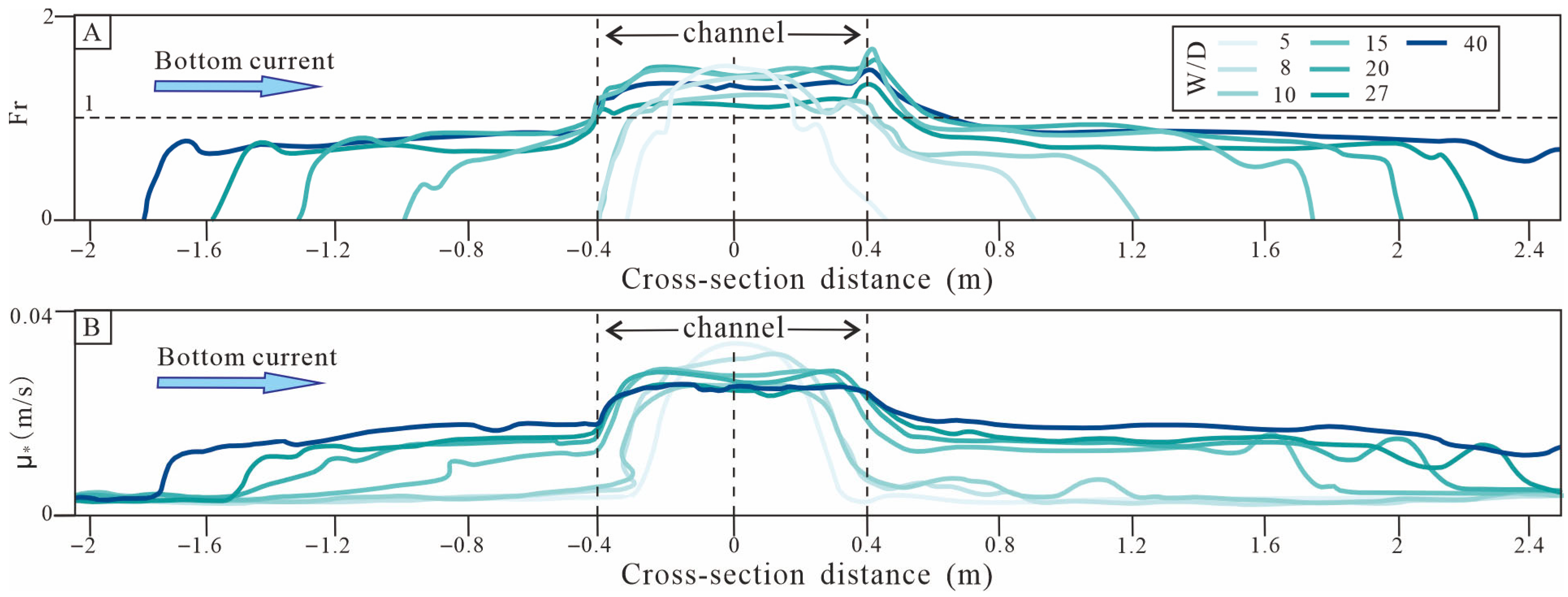
For each simulation case, this study calculated the average Froude number and Reynolds number across the entire flow domain (Table 3). The Froude number increased from 1.20 to 1.67 as the width-to-depth ratio increased. In the cross-stream direction, regardless of the channel confinement, the downstream side of the bottom current consistently exhibited higher Froude numbers and shear velocities within the channel interior. Inside the channel (from −0.4 m to 0.4 m), the Froude number was generally greater than 1, accompanied by relatively high shear velocities. Specifically, for smaller width-to-depth ratio, the maximum Froude number occurred near the channel centerline. In contrast, for larger width-to-depth ratios, the Froude number showed relatively uniform high values across the channel, with slightly lower values on the upstream side and a slightly higher peak on the downstream side of the bottom current. Outside the channel, the Froude number quickly decreased to below 1, and the shear velocity dropped significantly. Notably, as the width-to-depth ratio increased, the spatial extent where Fr > 0 expanded considerably, with this phenomenon being more pronounced on the downstream side of the bottom current (Figure 2A,B).

3.2. Flow Velocity

3.2.1. Down-Stream Velocity

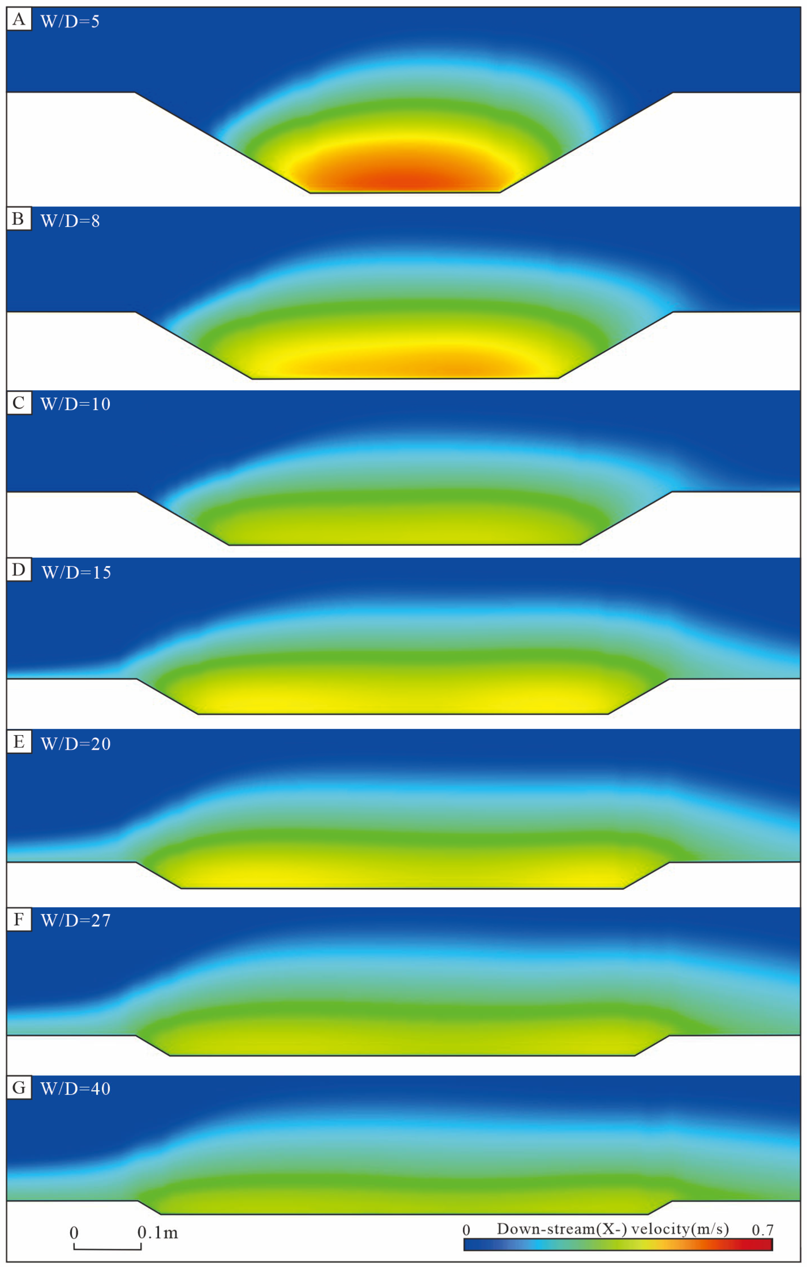
The distribution of down-stream velocity across the channel cross-section reflects the flow characteristics within channels with different width-to-depth ratios. In the color maps, areas ranging from blue to green represent lower flow velocities, while areas from yellow to red indicate higher velocities (Figure 3). For width-to-depth ratio of 5 and 8, the lower portion of the flow is predominantly yellow to red, with velocities around 0.4–0.5 m/s, while the upper portion is mainly green, with velocities between 0.1–0.3 m/s. At this stage, a distinct color stratification exists between the upper and lower parts, with a velocity difference exceeding 0.3 m/s (Figure 3A,B). As the width-to-depth ratio increases to 20–40, the lower part of the flow becomes green to light yellow, with velocities around 0.2–0.3 m/s. The color and velocity differences between this region and the light blue to green upper portion significantly diminish. The stratification becomes less distinct, overall velocities decrease, and the velocity difference between the upper and lower parts reduces to about 0.1 m/s (Figure 3E–G).
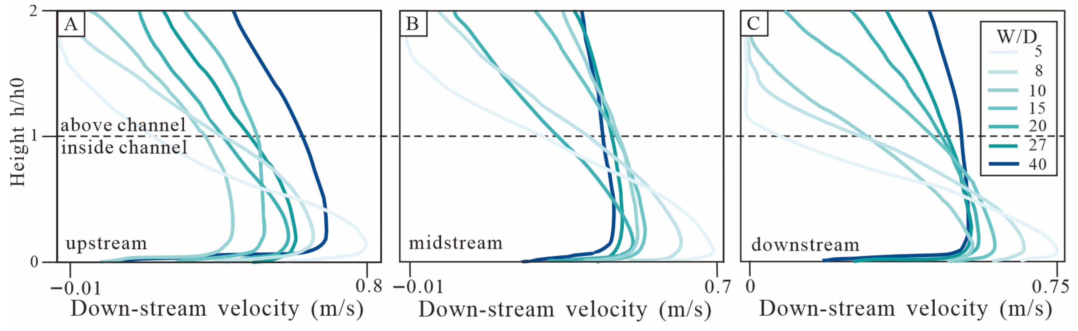
To further assess the impact of the bottom current on the channel flow, this investigation methodically collected downstream velocity profiles for various aspect ratios and studied their spatial development (Figure 4). The results show that as the width-to-depth ratio increases, the maximum downstream velocity decreases. In the upstream section of the channel (Figure 4A), the maximum velocity drops from 0.78 m/s at a width-to-depth ratio of 5 to 0.68 m/s at a ratio of 40; in the midstream section (Figure 4B), it decreases from 0.69 m/s to 0.45 m/s; and in the downstream section (Figure 4C), it decreases from 0.72 m/s to 0.54 m/s.
Furthermore, although the absolute depth-averaged flow thickness decreases with an increasing width-to-depth ratio, the dimensionless thickness relative to the channel height increases significantly as the ratio rises (Table 3, Figure 3 and Figure 4). The dimensionless flow thickness increases from less than 1 at a width-to-depth ratio of 5 to greater than 2 at a ratio of 40 (Figure 4). This trend further indicates that the vertical stratification effect of the flow weakens progressively as the channel width-to-depth ratio increases.

3.2.2. Cross-Stream Velocity

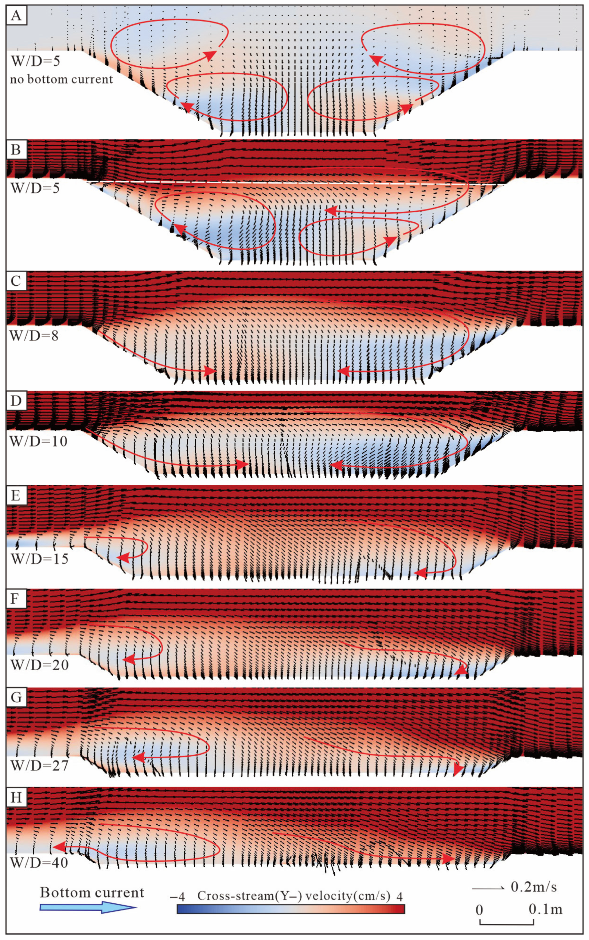
The cross-stream velocity distribution across the channel cross-section provides a clear representation of the evolution of the flow field as the width-to-depth ratio change (Figure 5). In the figure, red areas represent flow in the same direction as the bottom current, blue areas represent opposing flow, and the color intensity indicates the velocity magnitude. When the width-to-depth ratio is 5, a distinct interface exists between the bottom current above the channel and the flow within it (denoted by the white dashed line in Figure 5B), with clearly separated flow structures. Blue zones appear on both sides of the channel: the upstream blue zone is located near the channel bed, with a velocity of approximately −2.5 cm/s, while the downstream blue zone is positioned in mid-depth, with a velocity of about −1 cm/s (Figure 5B). As the width-to-depth ratio slightly increases the interaction between the turbidity current and the bottom current intensifies, causing their flow fields to gradually merge without a clear boundary. In this scenario, the blue zone within the channel is primarily located on the downstream side, with velocities ranging from −3 to −2 cm/s (Figure 5C–E). As the width-to-depth ratio continues to increase, the extent of the downstream blue zone gradually contracts, and its maximum velocity also weakens to about −1 cm/s. Simultaneously, a new blue zone begins to form on the upstream side, expanding progressively, with its maximum velocity increasing from approximately 0 cm/s to about −1 cm/s (Figure 5E–G). When the width-to-depth ratio reaches 40, the downstream blue zone largely disappears, leaving only a light blue area on the upstream side with a velocity of about −1 cm/s (Figure 5H).
The velocity vectors more clearly reveal the morphological evolution of the internal flow structure within the channel (Figure 5). The vector length represents the velocity magnitude, and the direction indicates the flow direction. When the width-to-depth ratio is 5, a pair of counter-rotating circulatory cells is present on both sides of the channel, similar in structure to the case without a bottom current (Figure 5A,B). As the width-to-depth ratio increases to 8–10, the flow fields on the two sides become asymmetric: a counter-flow secondary cell forms on the downstream side, while no significant cell forms on the upstream side (Figure 5C,D). As the width-to-depth ratio continues to increase from 10 to 27, the downstream circulatory cell gradually diminishes and is replaced by the direct influence of the bottom current, which flows in the same direction within the channel. Meanwhile, a new secondary cell begins to develop on the upstream side, extending beyond the channel confines when the width-to-depth ratio reaches 40 (Figure 5D–H).
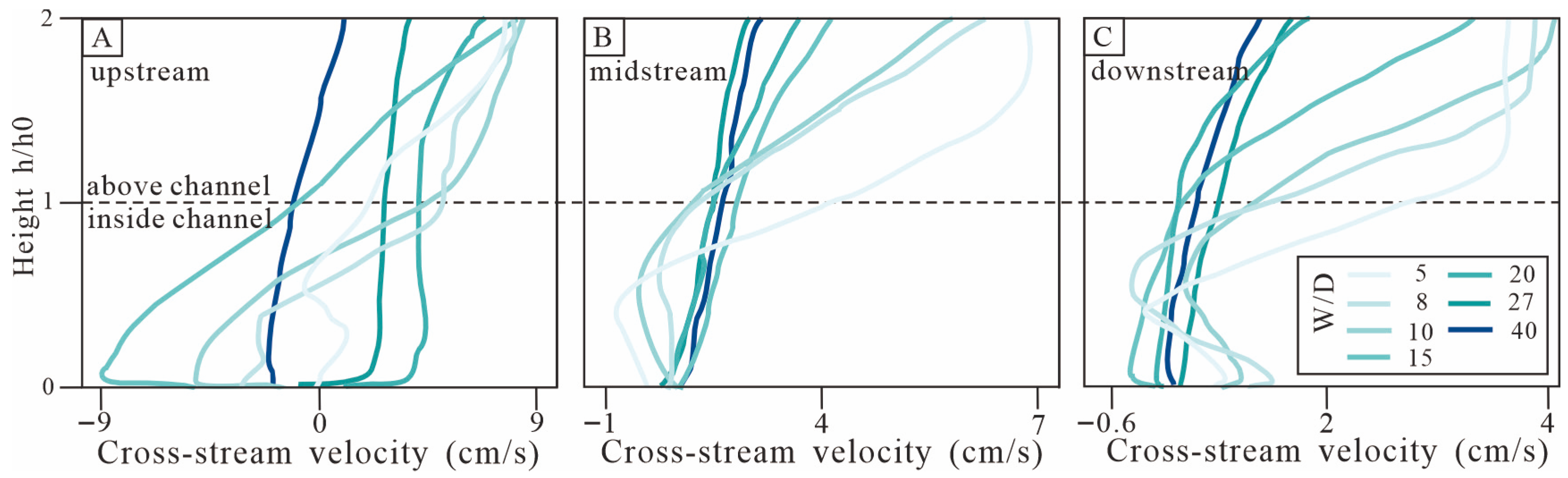
To more intuitively reveal the dynamic response of the flow above the channel under the influence of turbidity–bottom current interaction, this study systematically extracted the cross-stream velocity distributions for different width-to-depth ratios and analyzed their spatial evolution characteristics (Figure 6). The velocity profiles in the upstream region of the channel exhibit a more complex structure, while those in the midstream and downstream regions show clearer trends. When the width-to-depth ratio is small, the maximum cross-stream velocity of the flow is relatively large; as the ratio increases, this maximum velocity decreases. Specifically, in the upstream section (Figure 6A), the maximum velocity is 9 cm/s at a width-to-depth ratio of 5, but it decreases to 3 cm/s at a ratio of 40. In the midstream section (Figure 6B), the maximum velocity is 7 cm/s at a ratio of 5 and declines to 2 cm/s at a ratio of 40. In the downstream section (Figure 6C), the maximum velocity is 3.5 cm/s at a ratio of 5, reducing to 0.8 cm/s at a ratio of 40. Furthermore, from the upstream to the downstream sections of the channel, the maximum cross-stream velocity consistently decreases as the width-to-depth ratio increases.

3.3. Volumetric Concentration

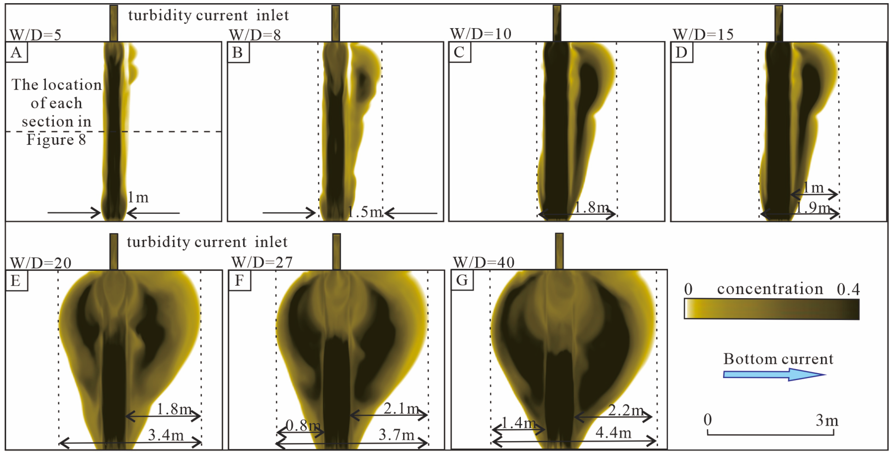
The planform distribution characteristics of fine-grained sediment concentration are shown in Figure 7. When the channel width-to-depth ratio is 5, sediment is largely confined within the channel, with only minor overspill toward the downstream side of the bottom current near the upstream outlet. The overall overspill effect is weak, with a maximum overspill distance reaching only 1 m (Figure 7A). As the width-to-depth ratio increases, the lateral extent of sediment overspill on both sides of the channel expands significantly, showing a decreasing trend along the channel, with the maximum overspill occurring in the upstream section. When the width-to-depth ratio reaches 40, the maximum overspill width increases to 4.4 m and the distribution has notable asymmetry, with the overspill extent about 2.2 m on the downstream side compared to 1.4 m on the upstream side (Figure 7G).
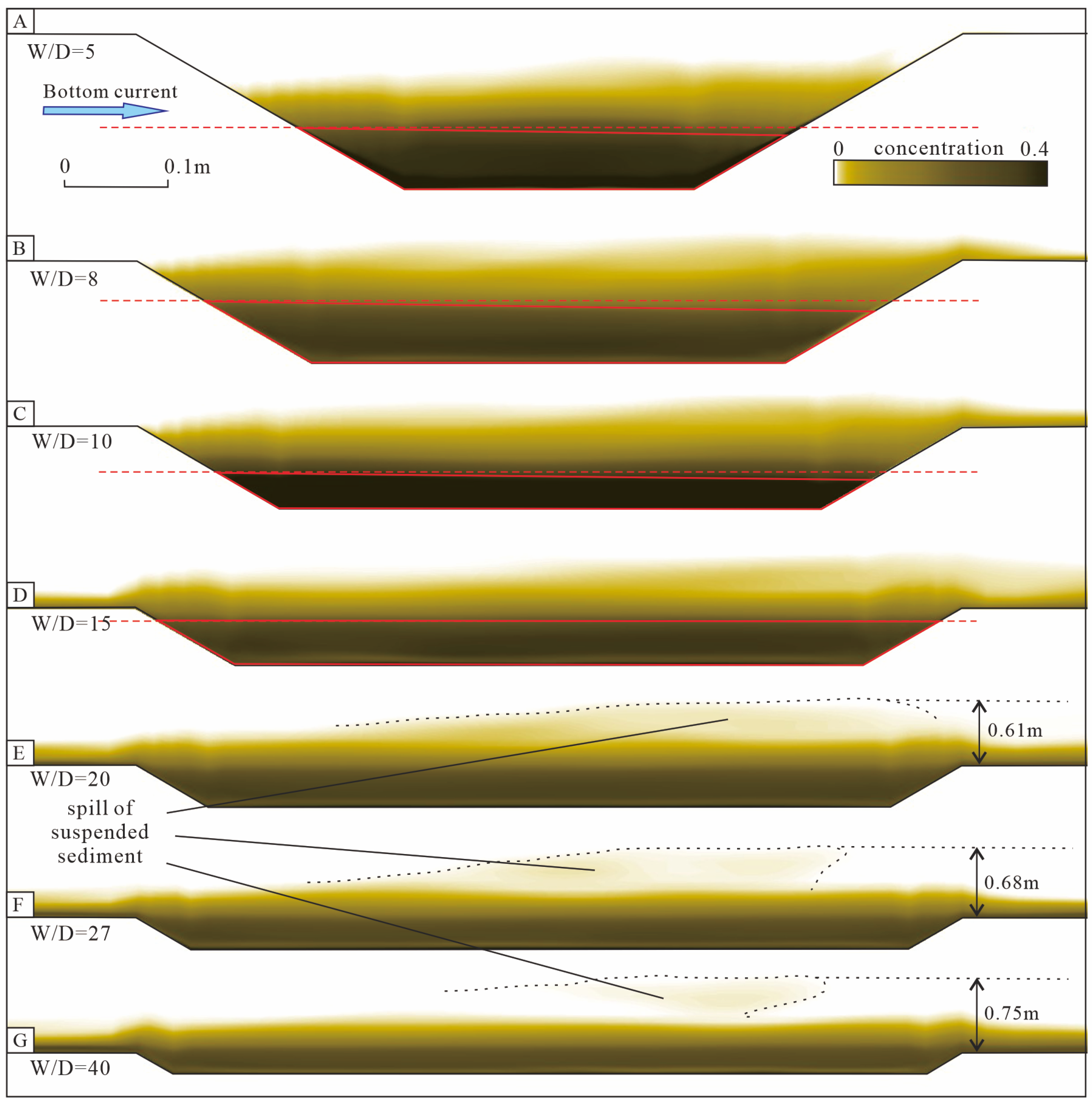
From the sediment concentration distribution across the channel cross-section (Figure 8), it is clear that, under the influence of the bottom current, the suspended sediment overall exhibits a deflection towards the downstream direction. This phenomenon is particularly pronounced in channels with a width-to-depth ratio greater than 20, as indicated by the black dashed line in Figure 8. As the width-to-depth ratio increases, the vertical extent of the sediment plume also expands. For instance, when the width-to-depth ratio is 20, the overspill height is 0.61 m; this increases to 0.75 m when the ratio reaches 40. For channels with a width-to-depth ratio less than 15, although suspended sediment in the upper layers still shows a tendency to deflect downstream, the near-bed concentration (indicated by the red solid line in Figure 8) exhibits an asymmetric pattern, with higher values upstream and lower values downstream. This pattern contrasts significantly with the horizontal reference line (red dashed line).

3.4. Fluid Density

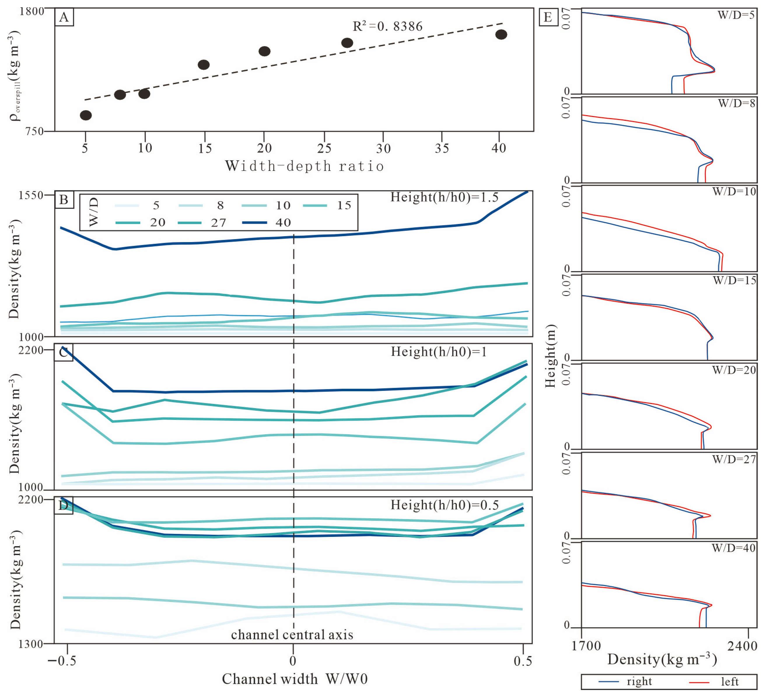
As the width-to-depth ratio increases, the average density of the overspill fluid shows a systematic increasing trend (Table 3, Figure 9A). In our simulations, there is a significant density contrast between the ambient fluid and the sediment particles. As a result, the fluid density directly reflects the sediment concentration it carries and can serve as an effective indicator for characterizing the spatial distribution of sediment. To systematically analyze the density distribution characteristics at different depths within the channel, Figure 9B–D illustrate the density variation along the down-stream direction for each simulation case. The channel width and depth in these figures are normalized to facilitate comparison of fluid density at different relative positions. The results show that channels with larger width-to-depth ratios exhibit higher fluid densities at the same relative height, and the high-density fluid also occupies a larger vertical extent. Specifically, at the height of 1.5 times the channel depth, only cases with a width-to-depth ratio greater than 27 maintain a relatively high average density (approximately 1400 kg/m3), with higher density observed on the downstream side of the bottom current. In other cases, the average density is close to that of the ambient fluid (1025 kg/m3). At the top of the channel (the height of 1 times the depth), the average density is approximately 1800 kg/m3 for cases with a width-to-depth ratio greater than 15, compared to about 1200 kg/m3 for cases with a ratio less than 15. At the height of 0.5 times the channel depth, the average density is approximately 2000 kg/m3 for cases with a ratio greater than 15 and about 1500 kg/m3 for those with a ratio less than 15 (Figure 9B–D). Further analysis of the density distribution at the same near-bed depth but across different lateral positions reveals a regular spatial pattern with varying width-to-depth ratio. When the ratio is less than 15, the density on the left side of the channel (red solid line) is higher than on the right side; conversely, when the ratio exceeds 15, the density on the right side (blue solid line) becomes greater (Figure 9E). This distribution characteristic is particularly pronounced in cases where the width-to-depth ratio is either less than 10 or greater than 27.

4. Discussion

4.1. The Impact of Varying Confinements on Turbidity–Bottom Current Interactions

Because the genesis of unidirectionally migrating channels arises from turbidity–bottom current interaction, investigating the influence of confinement on channel migration direction requires a clear understanding of how turbidity–bottom current interaction varies under different degrees of confinement.

4.1.1. The Strength of Interaction

Changes in dimensionless numbers such as the Froude number, effectively reflect the impact of external conditions on the dynamic processes of turbidity currents. Previous studies have suggested that an increase in the Froude number (Fr) typically indicates greater entrainment of ambient fluid into the turbidity current [41,50]. In these simulations, the ambient fluid is characterized as the lateral flow field that simulates the bottom current (Figure 3). Therefore, an increase in the Froude number signifies greater entrainment of the bottom current (as ambient fluid) into the turbidity current, leading to significant interaction between the two flows. These dimensionless numbers thus serve as effective indicators for the intensity of the interaction. Based on flume experiments, Adema et al. (2025a) [23] observed that under turbidity–bottom current interaction, as the channel width-to-depth ratio increased from 8 to 20, the Froude number of the flow within the channel increased from 1.6 to 1.9. Similarly, our simulations show a trend of increasing average Froude number as the width-to-depth ratio increases (Table 3). When channel confinement is strong (with a small width-to-depth ratio), the entrainment of the bottom current primarily occurs near the channel center. In contrast, as confinement weakens, the entrainment process shifts predominantly toward the channel sides, with the spatial extent available for bottom current entrainment also increasing (Figure 2). Moreover, in this study, the average Froude number ranges approximately from 1.2 to 1.73, which aligns with the Froude numbers (from 1.25 to 2.05) calculated by Chen et al. (2020) [11] for turbidity–bottom current interaction using sand-body geometric parameters from the Rovuma Basin. This indicates that the present simulations can, to some extent, reflect the fluid properties under real-world conditions.

4.1.2. Transporting Sediment Flow

Variations in channel confinement, driven by differing intensities of the interaction, lead to significant differences in the morphology of secondary flows and the distribution of flow velocities (Figure 5). It has been proposed that the formation mechanisms of secondary flows can be categorized into two main types: one arising from pressure gradients or centrifugal forces, and the other driven by the anisotropy of turbulence [51].
When the width-to-depth ratio is extremely small, the secondary flow pattern in the middle and lower parts of the channel resembles the secondary flow structure observed in straight channels without the influence of bottom currents (Figure 5A,B). Additionally, the maximum Froude number is located at the channel center (Figure 2). At this stage, the primary distinction between scenarios with and without a bottom current is that, in the presence of a bottom current, the circulatory cell on the upstream side is slightly stronger, and the secondary flow in the upper part of the channel aligns with the direction of the bottom current. The interaction at this point is weak, and the bottom current above the channel does not significantly alter the dynamic characteristics of the turbidity current in the middle and lower parts of the channel. In the mid-lower sections of straight channels, turbidity currents generate symmetrical secondary flows due to turbulence, which aligns with the secondary circulation model dominated by turbulence anisotropy, as proposed in previous studies [52,53,54]. In this study, the Reynolds number for all simulation cases ranges between 20,000 and 45,000, indicating significant turbulence effects (Table 3). Therefore, the circulation at this stage can be attributed to turbulence anisotropy.
As the width-to-depth ratio increases, the influence of the bottom current on the secondary flow gradually strengthens. Chen et al. (2020) [11] suggested that bottom currents may modulate the structure of secondary flows. Adema et al. (2025a) [23] further argued that, at this stage, the secondary flow is primarily generated by the shear stress gradient between the bottom current and the turbidity current, rather than by turbulence anisotropy, leading to changes in the flow direction and location of the circulatory cell. In our simulations, as the width-to-depth ratio increases, the location of the maximum Froude number shifts from the channel center towards the downstream side of the bottom current, and the Froude number values at both sides of the channel increase (Figure 2). This indicates that the channel sides experience a stronger and more asymmetric interaction. This change directly alters the secondary flow structure: a counter-rotating secondary flow cell concentrates on the downstream side of the bottom current, while no significant cell develops on the upstream side (Figure 5C,D). This pattern is consistent with the circulation features documented by Gong et al. (2016) [7], where the secondary flow originates from the downstream side and points upstream relative to the bottom current.
As the width-to-depth ratio continues to increase, the intensified interaction causes the secondary flow on the downstream side of the bottom current to gradually weaken and eventually disappear. The downstream region of the channel begins to be directly controlled by a flow field aligned with the bottom current direction. This phenomenon aligns with the observation by Adema et al. (2025a) [23] that the secondary flow initially located downstream weakens and vanishes as the width-to-depth ratio increases. Meanwhile, a new secondary flow cell gradually develops on the upstream side of the bottom current (Figure 5E–H), though its intensity remains relatively weak. Correspondingly, within the same simulation case, the Froude number on the upstream side of the bottom current is lower than that on the downstream side (Figure 2), indicating that at this stage, the flow dynamics are primarily governed by the direct influence of the downstream side of the bottom current.
In summary, as the channel width-to-depth ratio increases from small to large, the flow structure undergoes the following sequential evolution: initially dominated by symmetrical secondary flows driven by turbulence anisotropy; then transitioning to secondary circulation driven by shear stress gradients, developing only on the downstream side of the bottom current; and finally evolving into a flow field morphology directly controlled by the bottom current.

4.1.3. Near-Seabed Sediment

Both sediment concentration and fluid density are key indicators for characterizing the depositional features of turbidity currents [32,41,55]. Due to the significantly higher density of the particle phase compared to the ambient fluid (Table 2), variations in the width-to-depth ratio lead to differences in the dynamic properties of the sediment-laden flow. These differences, in turn, influence near-seabed depositional processes and shape the style of lateral sediment stacking.
When the width-to-depth ratio is small, the peak shear velocity is located near the channel center, slightly shifted towards the downstream side of the bottom current (Figure 2B). The lower shear velocity on the upstream side of the bottom current favors the settling of sediment near the bed. Under these conditions, the near-bed concentration contour (red solid line in Figure 8) exhibits higher values upstream and lower values downstream. Correspondingly, fluid density near the seabed is also higher on the upstream side of the bottom current compared to the downstream side (Figure 9E). This indicates that near-seabed sediment is transported upstream by the near-bed flow, resulting in a thicker deposit upstream, as described by Gong et al. (2016) [7].
In contrast to cases with width-to-depth ratios of 5–10, cases with ratios of 15–40 exhibit higher shear velocities on the upstream side of the bottom current (Figure 2B). Although a secondary flow opposing the bottom current direction persists upstream (Figure 5), the increased shear stress hinders significant sediment accumulation in this area. This is evident from the sediment concentration maps, where the near-bed concentration contour in Figure 8 gradually becomes more horizontal, indicating that near-seabed sediment is no longer being transported significantly upstream. Conversely, with enhanced interaction, the fluid density near the seabed is higher on the downstream side of the bottom current (Figure 9E), and the channel flow field becomes increasingly dominated by the direct influence of the bottom current (see Section 4.1.2). It is noteworthy that near-seabed sediment transport and near-wall treatment in the field of CFD do not operate at the same scale. As can be roughly observed from Figure 4, the viscous sublayer is confined to heights where h/h0 < 0.1. However, in Figure 9E, which is used to quantitatively characterize differences in near-seabed sediment transport, density contrasts between the two sides of the channel persist even at heights where h/h0 > 0.3 that already falls within the logarithmic layer. Therefore, sediment transport differences still exist in the lower part of the logarithmic layer. Relative to the entire channel, this transport discrepancy is located close to the channel bed and is thus referred to as near-seabed sediment transport variation.
As a result, near-seabed sediment is increasingly deflected downstream. This phenomenon of downstream sediment deflection aligns with the Drift Deposition Model proposed by Fonnesu et al. (2020) [12], which has been validated by flume experiments [28]. The transition in depositional mode induced by changes in the width-to-depth ratio described that, as the ratio increases, the dominant transport direction of near-seabed sediment gradually shifts from upstream to downstream.

4.1.4. Suspended Sediment

In studies of turbidity currents, higher shear velocity typically indicates that sediment is more likely to remain in suspension and is prone to overspill [25,41,56]. Wells and Dorrell (2021) [39] proposed that fluid stratification induced by sediment settling within turbidity currents can dampen turbulence development, leading to a decrease in the Froude number. Similarly, Serra et al. (2025) [54] argued that as turbidity currents undergo continuous mixing and settling, the inertial scale effects gradually weaken, resulting in a corresponding decrease in the Froude number. Thus, a decrease in the Froude number can indicate a tendency for net particle settling, while an increase suggests net particle suspension. In this study, as the width-to-depth ratio increases, the depth-averaged shear velocity, average Froude number, and Reynolds number of the flow all increase (Table 3). This suggests that, compared to channels with a smaller width-to-depth ratio, particles in channels with a larger ratio are more likely to remain suspended and experience overspill. Additionally, the depth-averaged height (h) decreases as the width-to-depth ratio increases (Table 3), indicating a weakening of flow stratification (Figure 3 and Figure 4). This further supports the trend of enhanced suspension, as indicated by the rising Froude number. In channels with larger width-to-depth ratios, sediment remains in a more suspension state, making it more susceptible to being driven by the bottom current, which results in an overall downstream deflection.
Since the Froude number in this study is calculated based on sediment concentration, the spatial extent where Fr > 0 outside the channel can be used to indicate the area of suspended sediment overspill. The results show that cases with larger width-to-depth ratios exhibit larger Fr > 0 regions, which corresponds to greater overspill distances for the sediment (Figure 2) and the formation of overspill deposits [12]. This trend is further supported by the increasing average density of the overspill fluid with larger width-to-depth ratios (Figure 9A). At the same relative depth, cases with larger width-to-depth ratios exhibit higher fluid densities (Figure 9B–D), reflecting greater concentrations and a larger vertical extent of overspilled sediment (Figure 7 and Figure 8). Collectively, this evidence demonstrates that sediment generally overspills and deflects downstream under the influence of the bottom current, and the channel width-to-depth ratio directly governs the spatial magnitude of this sediment overspill.

4.2. The Role of Confinement in Channel Unidirectionally Migration

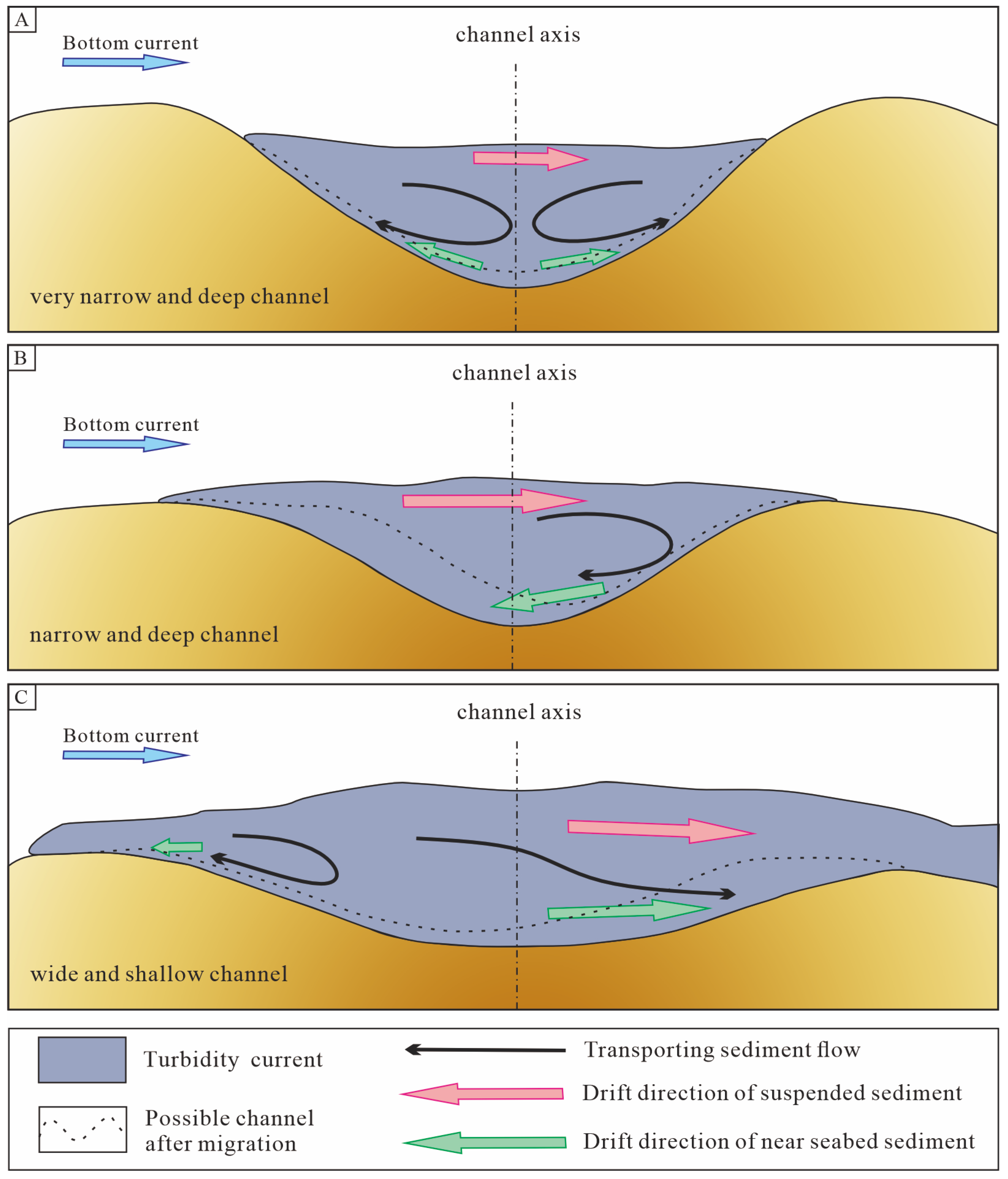
Flow properties and depositional trends within channels exhibit significant differences under varying width-to-depth ratios. By synthesizing the influence of confinement on the interaction in straight channels, this study proposes three mechanisms through which confinement governs channel migration direction.

4.2.1. Strong Confinement at Very Small Width-to-Depth Ratios

At this stage, the interaction within the channel is weak (Figure 2), and the secondary flow is primarily dominated by turbulence anisotropy. This manifesting as a pair of symmetrical, counter-rotating cells on both sides of the channel (Figure 5). Sediment overspill is minimal, and the depositional pattern resembles that of straight turbidity current channels without the influence of bottom current (Figure 7, Figure 8 and Figure 9). Previous studies have indicated that straight turbidity current channels typically lack the capacity for spontaneous unidirectional migration [57,58]. Correspondingly, channels at this stage also show no significant lateral migration trend (Figure 10A).

4.2.2. Moderate Confinement

As the interaction gradually intensifies (Figure 2), the secondary flow becomes dominated by the shear stress gradient between the bottom current and the turbidity current. While a portion of suspended sediment overspills in the downstream direction of the bottom current, near-seabed sediment is transported upstream by the secondary flow and deposited (Figure 5, Figure 6, Figure 7, Figure 8 and Figure 9). Over time, this process promotes overall channel migration in the downstream direction (Figure 10B). The secondary flow, which transports near-seabed sediment from the downstream to the upstream side of the bottom current, matches the flow direction and distribution position of the secondary flow [23]. Furthermore, the width-to-depth ratios of 8–15 used in this study are similar to those in their experimental cases (ratios of 8 and 11.4). This secondary flow pattern is also consistent with the model proposed by Gong et al. (2016) [7], based on seismic data.

4.2.3. Weak Confinement at Large Width-to-Depth Ratios

At this stage, the interaction is strong (Figure 2), and the flow is primarily governed by the bottom current. The transverse flow on the downstream side aligns with the direction of the bottom current, driving sediment drift deposition downstream (Figure 5, Figure 6, Figure 7, Figure 8 and Figure 9). A weak secondary flow develops on the upstream side, capable of transporting a small amount of sediment out of the channel (Figure 5). Over time, this mechanism leads to the channel exhibiting an overall upstream migration characteristic (Figure 10C). This mode, in which near-seabed sediment is transported directly downstream by the bottom current [12], and the drift process was demonstrated in the flume experiments of Miramontes et al. (2020) [28].
The above mechanisms indicate that variations in the channel width-to-depth ratio can lead to three distinct geomorphological evolution modes—negligible migration, downstream migration, and upstream migration—by altering the sedimentary dynamic processes.

5. Conclusions

Based on numerical simulation experiments, this study successfully reproduced the turbidity–bottom current interaction and systematically discussed the influence of various channel confinement parameters on this process. The model reveals a dynamic mechanism controlling channel morphological evolution by influencing the lateral sediment stacking trend, providing a new explanation for the long-standing debate regarding the evolutionary mechanisms of unidirectionally migrating channels. The research confirms that both downstream- and upstream-migrating channels can develop under actual geological conditions, unifying various previously proposed mechanisms and showing consistency with field data from seismic profiles.
(1) Variations in Channel Confinement: Changes in channel confinement modulate the intensity of the turbidity–bottom current interaction, thereby altering the flow velocity distribution and the structure of the secondary circulation within the channel. These changes ultimately affect the dynamic response of near-seabed sediment. As the width-to-depth ratio increases and the interaction strengthens, the dominant location of the secondary flow within the channel shifts from the downstream side to the upstream side of the bottom current. Correspondingly, the predominant transport direction of near-seabed sediment transitions from upstream deflection to downstream deflection relative to the bottom current.
(2) Highly Confined Channels: In highly confined channels, the influence of the bottom current is primarily restricted to the region above the channel while the turbidity current is largely confined within the channel. This results in a very weak interaction between the two. The flow behavior inside the channel resembles that of a turbidity current without a bottom current, dominated by turbulence-anisotropy-driven secondary flow. Consequently, these channels exhibit negligible lateral migration.
(3) Moderately Confined Channels: In moderately confined channels, which have a relatively small width-to-depth ratio, the bottom current can significantly influence the turbidity current. Under this interaction, a secondary circulation driven by the shear stress difference between the bottom current and the turbidity current develops on the downstream side of the channel. This flow transports near-seabed sediment from the downstream side towards the upstream side for deposition, promoting overall downstream channel migration.
(4) Weakly Confined Channels: In weakly confined channels, which have large width-to-depth ratios, the turbidity–bottom current interaction is strong. The bottom current descends directly after bypassing the channel wall, transporting and depositing sediment downstream. Meanwhile, a very weak secondary flow develops on the upstream side. This mechanism leads to a tendency for upstream channel migration.
This research provides a novel perspective on channel migration mechanisms, demonstrating that the migration process is governed by morphodynamic feedback. It offers valuable insights into the evolution of deep-sea sedimentary geomorphology. However, it should be noted that the turbidity–bottom current interaction is a complex process, and the channel width-to-depth ratio is not the sole factor influencing sediment lateral stacking and channel migration direction. In nature geological systems, factors such as the Coriolis force, channel sinuosity, continental slope gradient, and the relative scales of the turbidity and bottom currents may also play significant roles in governing the direction of migration. The specific factors involved and their coupled effects warrant further investigation in subsequent studies.

Supplementary Materials

The following supporting information can be downloaded at: https://www.mdpi.com/article/10.3390/jmse14020152/s1, Figure S1: (A) Flume model. The blue section represents the Eurotank flume model used for model validation, while the green section indicates the model used in the simulations. (B) Channel model used for model validation. The location of the cross-section is shown in Figure S1A.

Author Contributions

R.Z.: Writing—original draft, Conceptualization, Methodology, Software, Data curation, Investigation, Visualization, and Formal analysis. D.T.: Writing—review & editing, Writing—original draft, Methodology, Validation, Software, Investigation, Funding acquisition, and Visualization. X.L.: Writing—review & editing, Writing—original draft, Conceptualization, Supervision, Funding acquisition, Data curation, Resources, and Project administration. T.A.: Writing—review & editing. J.W.: Writing—review & editing. T.J.: Writing—review & editing and Software. G.L.: Writing—review & editing. X.X.: Writing—review & editing. All authors have read and agreed to the published version of the manuscript.

Funding

This research was funded by the National Natural Science Foundation of China (Nos. 42130408 and 42502098).

Data Availability Statement

Data will be made available on request, due to the fact that the relevant simulation files are too large and prone to damage when compressed.

Conflicts of Interest

The authors declare that they have no known competing financial interests or personal relationships that could have appeared to influence the work reported in this paper. Author J.W. comes from the Petroleum China Hangzhou Research Institute of Petroleum Geology, but in this study, he participated as a scholar rather than a sponsor. Petroleum China has no potential commercial interests in this study.

References

  1. Rebesco, M.; Hernández-Molina, F.J.; Van Rooij, D.; Wåhlin, A. Contourites and Associated Sediments Controlled by Deep-Water Circulation Processes: State-of-the-Art and Future Considerations. Mar. Geol. 2014, 352, 111–154. [Google Scholar] [CrossRef]
  2. Mulder, T.; Faugères, J.-C.; Gonthier, E. Mixed Turbidite–Contourite Systems. In Developments in Sedimentology; Elsevier: Amsterdam, The Netherlands, 2008; Volume 60, pp. 435–456. [Google Scholar] [CrossRef]
  3. Rodrigues, S.; Hernández-Molina, F.J.; Fonnesu, M.; Miramontes, E.; Rebesco, M.; Campbell, D.C. A New Classification System for Mixed (Turbidite-Contourite) Depositional Systems: Examples, Conceptual Models and Diagnostic Criteria for Modern and Ancient Records. Earth-Sci. Rev. 2022, 230, 104030. [Google Scholar] [CrossRef]
  4. Rasmussen, E.S. The Relationship between Submarine Canyon Fill and Sea-Level Change: An Example from Middle Miocene Offshore Gabon, West Africa. Sediment. Geol. 1994, 90, 61–75. [Google Scholar] [CrossRef]
  5. Calvin Campbell, D.; Mosher, D.C. Geophysical Evidence for Widespread Cenozoic Bottom Current Activity from the Continental Margin of Nova Scotia, Canada. Mar. Geol. 2016, 378, 237–260. [Google Scholar] [CrossRef]
  6. Rodrigues, S.; Deptuck, M.E.; Kendell, K.L.; Campbell, C.; Hernández-Molina, F.J. Cretaceous to Eocene Mixed Turbidite-Contourite Systems Offshore Nova Scotia (Canada): Spatial and Temporal Variability of down- and along-Slope Processes. Mar. Pet. Geol. 2022, 138, 105572. [Google Scholar] [CrossRef]
  7. Gong, C.; Wang, Y.; Steel, R.J.; Peakall, J.; Zhao, X.; Sun, Q. Flow Processes and Sedimentation in Unidirectionally Migrating Deep-water Channels: From a Three-dimensional Seismic Perspective. Sedimentology 2016, 63, 645–661. [Google Scholar] [CrossRef]
  8. Zhu, M.; Graham, S.; Pang, X.; McHargue, T. Characteristics of Migrating Submarine Canyons from the Middle Miocene to Present: Implications for Paleoceanographic Circulation, Northern South China Sea. Mar. Pet. Geol. 2010, 27, 307–319. [Google Scholar] [CrossRef]
  9. He, Y.; Xie, X.; Kneller, B.C.; Wang, Z.; Li, X. Architecture and Controlling Factors of Canyon Fills on the Shelf Margin in the Qiongdongnan Basin, Northern South China Sea. Mar. Pet. Geol. 2013, 41, 264–276. [Google Scholar] [CrossRef]
  10. Gong, C.; Wang, Y.; Zhu, W.; Li, W.; Xu, Q. Upper Miocene to Quaternary Unidirectionally Migrating Deep-Water Channels in the Pearl River Mouth Basin, Northern South China Sea. Bulletin 2013, 97, 285–308. [Google Scholar] [CrossRef]
  11. Chen, Y.; Yao, G.; Wang, X.; Lv, F.; Shao, D.; Lu, Y.; Cao, Q.; Tang, P. Flow Processes of the Interaction between Turbidity Flows and Bottom Currents in Sinuous Unidirectionally Migrating Channels: An Example from the Oligocene Channels in the Rovuma Basin, Offshore Mozambique. Sediment. Geol. 2020, 404, 105680. [Google Scholar] [CrossRef]
  12. Fonnesu, M.; Palermo, D.; Galbiati, M.; Marchesini, M.; Bonamini, E.; Bendias, D. A New World-Class Deep-Water Play-Type, Deposited by the Syndepositional Interaction of Turbidity Flows and Bottom Currents: The Giant Eocene Coral Field in Northern Mozambique. Mar. Pet. Geol. 2020, 111, 179–201. [Google Scholar] [CrossRef]
  13. Rebesco, M.; Larter, R.D.; Camerlenghi, A.; Barker, P.F. Giant Sediment Drifts on the Continental Rise West of the Antarctic Peninsula. Geo-Mar. Lett. 1996, 16, 65–75. [Google Scholar] [CrossRef]
  14. Rodrigues, S.; Hernández-Molina, F.J.; Larter, R.D.; Rebesco, M.; Hillenbrand, C.-D.; Lucchi, R.G.; Rodríguez-Tovar, F.J. Sedimentary Model for Mixed Depositional Systems along the Pacific Margin of the Antarctic Peninsula: Decoding the Interplay of Deep-Water Processes. Mar. Geol. 2022, 445, 106754. [Google Scholar] [CrossRef]
  15. Rodrigues, S.; Hernández-Molina, F.J.; Kirby, A. A Late Cretaceous Mixed (Turbidite-Contourite) System along the Argentine Margin: Paleoceanographic and Conceptual Implications. Mar. Pet. Geol. 2021, 123, 104768. [Google Scholar] [CrossRef]
  16. Mourlot, Y.; Calvès, G.; Clift, P.D.; Baby, G.; Chaboureau, A.-C.; Raisson, F. Seismic Stratigraphy of Cretaceous Eastern Central Atlantic Ocean: Basin Evolution and Palaeoceanographic Implications. Earth Planet. Sci. Lett. 2018, 499, 107–121. [Google Scholar] [CrossRef]
  17. Lu, H.; Fulthorpe, C.S.; Mann, P. Three-Dimensional Architecture of Shelf-Building Sediment Drifts in the Offshore Canterbury Basin, New Zealand. Mar. Geol. 2003, 193, 19–47. [Google Scholar] [CrossRef]
  18. Gong, C.; Wang, Y.; Rebesco, M.; Salon, S.; Steel, R.J. How Do Turbidity Flows Interact with Contour Currents in Unidirectionally Migrating Deep-Water Channels? Geology 2018, 46, 551–554. [Google Scholar] [CrossRef]
  19. Rasmussen, S.; Lykke-Andersen, H.; Kuijpers, A.; Troelstra, S.R. Post-Miocene Sedimentation at the Continental Rise of Southeast Greenland: The Interplay between Turbidity and Contour Currents. Mar. Geol. 2003, 196, 37–52. [Google Scholar] [CrossRef]
  20. Sansom, P. Hybrid Turbidite–Contourite Systems of the Tanzanian Margin. Pet. Geosci. 2018, 24, 258–276. [Google Scholar] [CrossRef]
  21. Kolla, V. A Review of Sinuous Channel Avulsion Patterns in Some Major Deep-Sea Fans and Factors Controlling Them. Mar. Pet. Geol. 2007, 24, 450–469. [Google Scholar] [CrossRef]
  22. Eggenhuisen, J.T.; Mccaffrey, W.D.; Haughton, P.D.W.; Butler, R.W.H. Shallow Erosion beneath Turbidity Currents and Its Impact on the Architectural Development of Turbidite Sheet Systems. Sedimentology 2011, 58, 936–959. [Google Scholar] [CrossRef]
  23. Adema, P.H.; Eggenhuisen, J.T.; Bleeker, J.; Jacinto, R.S.; Miramontes, E. Turbidity Current Flow Structure and Its Modulation by Contour Currents: Insights from 3D Flume Experiments. Mar. Geol. 2025, 480, 107469. [Google Scholar] [CrossRef]
  24. Adema, P.H.; Eggenhuisen, J.T.; Jacinto, R.S.; Lagunova, N.; Alwadhakhi, A.I.; Van Der Woning, R.; Miramontes, E. Submarine Channel Shape Controls Combined Turbidity Current–Contour Current Flow. Mar. Geol. 2025, 490, 107646. [Google Scholar] [CrossRef]
  25. De Leeuw, J.; Eggenhuisen, J.T.; Cartigny, M.J.B. Morphodynamics of Submarine Channel Inception Revealed by New Experimental Approach. Nat. Commun. 2016, 7, 10886. [Google Scholar] [CrossRef]
  26. Georgoulas, A.N.; Angelidis, P.B.; Panagiotidis, T.G.; Kotsovinos, N.E. 3D Numerical Modelling of Turbidity Currents. Environ. Fluid Mech. 2010, 10, 603–635. [Google Scholar] [CrossRef]
  27. Giorgio Serchi, F.; Peakall, J.; Ingham, D.B.; Burns, A.D. A Unifying Computational Fluid Dynamics Investigation on the River-like to River-Reversed Secondary Circulation in Submarine Channel Bends. J. Geophys. Res. 2011, 116, C06012. [Google Scholar] [CrossRef]
  28. Miramontes, E.; Eggenhuisen, J.T.; Jacinto, R.S.; Poneti, G.; Pohl, F.; Normandeau, A.; Campbell, D.C.; Hernández-Molina, F.J. Channel-Levee Evolution in Combined Contour Current–Turbidity Current Flows from Flume-Tank Experiments. Geology 2020, 48, 353–357. [Google Scholar] [CrossRef]
  29. Gladstone; Phillips; Sparks. Experiments on Bidisperse, Constant-volume Gravity Currents: Propagation and Sediment Deposition. Sedimentology 1998, 45, 833–843. [Google Scholar] [CrossRef]
  30. Ezz, H.; Imran, J. Curvature-Induced Secondary Flow in Submarine Channels. Environ. Fluid Mech. 2014, 14, 343–370. [Google Scholar] [CrossRef]
  31. Tian, D.; Jiang, T.; Cao, L.; Pei, J.; Liao, J.; Meiburg, E. Numerical Modeling of Flow Structure and Sedimentation to Explain the Force Balance in Sinuous Submarine Channels. Mar. Geophys. Res. 2025, 46, 26. [Google Scholar] [CrossRef]
  32. Ellison, T.H.; Turner, J.S. Turbulent Entrainment in Stratified Flows. J. Fluid Mech. 1959, 6, 423–448. [Google Scholar] [CrossRef]
  33. Cantero, M.I.; Balachandar, S.; García, M.H.; Bock, D. Turbulent Structures in Planar Gravity Currents and Their Influence on the Flow Dynamics. J. Geophys. Res. Oceans 2008, 113, 2007JC004645. [Google Scholar] [CrossRef]
  34. Amos, K.J.; Peakall, J.; Bradbury, P.W.; Roberts, M.; Keevil, G.; Gupta, S. The Influence of Bend Amplitude and Planform Morphology on Flow and Sedimentation in Submarine Channels. Mar. Pet. Geol. 2010, 27, 1431–1447. [Google Scholar] [CrossRef]
  35. Sequeiros, O.E.; Spinewine, B.; Beaubouef, R.T.; Sun, T.; García, M.H.; Parker, G. Characteristics of Velocity and Excess Density Profiles of Saline Underflows and Turbidity Currents Flowing over a Mobile Bed. J. Hydraul. Eng. 2010, 136, 412–433. [Google Scholar] [CrossRef]
  36. Fildani, A.; Normark, W.R.; Kostic, S.; Parker, G. Channel Formation by Flow Stripping: Large-scale Scour Features along the Monterey East Channel and Their Relation to Sediment Waves. Sedimentology 2006, 53, 1265–1287. [Google Scholar] [CrossRef]
  37. Yang, Y.; Wang, D.; Kneller, B.; Zhong, G.; Yu, K.; Wang, M.; Xu, J. How Does Plastic Litter Accumulate in Submarine Canyons? Geophys. Res. Lett. 2024, 51, e2024GL110767. [Google Scholar] [CrossRef]
  38. Eggenhuisen, J.T.; Cartigny, M.J.B.; De Leeuw, J. Physical Theory for Near-Bed Turbulent Particle Suspension Capacity. Earth Surf. Dyn. 2017, 5, 269–281. [Google Scholar] [CrossRef]
  39. Wells, M.G.; Dorrell, R.M. Turbulence Processes within Turbidity Currents. Annu. Rev. Fluid Mech. 2021, 53, 59–83. [Google Scholar] [CrossRef]
  40. Huang, H.; Imran, J.; Pirmez, C. Numerical Model of Turbidity Currents with a Deforming Bottom Boundary. J. Hydraul. Eng. 2005, 131, 283–293. [Google Scholar] [CrossRef]
  41. Abd El-Gawad, S.; Cantelli, A.; Pirmez, C.; Minisini, D.; Sylvester, Z.; Imran, J. Three-dimensional Numerical Simulation of Turbidity Currents in a Submarine Channel on the Seafloor of the Niger Delta Slope. J. Geophys. Res. Oceans 2012, 117, 2011JC007538. [Google Scholar] [CrossRef]
  42. Jiang, T.; Zhang, Y.; Tang, S.; Zhang, D.; Zuo, Q.; Lin, W.; Wang, Y.; Sun, H.; Wang, B. CFD Simulation on the Generation of Turbidites in Deepwater Areas: A Case Study of Turbidity Current Processes in Qiongdongnan Basin, Northern South China Sea. Acta Oceanol. Sin. 2014, 33, 127–137. [Google Scholar] [CrossRef]
  43. Khalaf, M.; Kim, H.; Sun, A.Y.; Van Essendelft, D.; Shih, C.Y.; Liu, G.; Siriwardane, H. High-Performance Reservoir Simulation with Wafer-Scale Engine for Large-Scale Carbon Storage. Energies 2025, 18, 5874. [Google Scholar] [CrossRef]
  44. Huang, H.; Imran, J.; Pirmez, C. The Depositional Characteristics of Turbidity Currents in Submarine Sinuous Channels. Mar. Geol. 2012, 329–331, 93–102. [Google Scholar] [CrossRef]
  45. Kuijpers, A.; Troelstra, S.R.; Prins, M.A.; Linthout, K.; Akhmetzhanov, A.; Bouryak, S.; Bachmann, M.F.; Lassen, S.; Rasmussen, S.; Jensen, J.B. Late Quaternary Sedimentary Processes and Ocean Circulation Changes at the Southeast Greenland Margin. Mar. Geol. 2003, 195, 109–129. [Google Scholar] [CrossRef]
  46. Tian, D.; Jiang, T.; Wang, H.; Zhang, D.; Meiburg, E. Flow Dynamics and Sedimentation at a Turbidity Channel Confluence in the Yinggehai Basin, Northwestern South China Sea. Geoenergy Sci. Eng. 2023, 227, 211927. [Google Scholar] [CrossRef]
  47. Straub, K.M.; Mohrig, D.; Buttles, J.; McElroy, B.; Pirmez, C. Quantifying the Influence of Channel Sinuosity on the Depositional Mechanics of Channelized Turbidity Currents: A Laboratory Study. Mar. Pet. Geol. 2011, 28, 744–760. [Google Scholar] [CrossRef]
  48. Cenedese, C.; Adduce, C. A New Parameterization for Entrainment in Overflows. J. Phys. Oceanogr. 2010, 40, 1835–1850. [Google Scholar] [CrossRef]
  49. Prandtl, L. Essentials of Fluid Dynamics; Hafner Publishing Company: New York, NY, USA, 1952. [Google Scholar]
  50. Hinze, J.O. Experimental Investigation on Secondary Currents in the Turbulent Flow through a Straight Conduit. Appl. Sci. Res. 1973, 28, 453–465. [Google Scholar] [CrossRef]
  51. Wang, Z.-Q.; Cheng, N.-S. Time-Mean Structure of Secondary Flows in Open Channel with Longitudinal Bedforms. Adv. Water Resour. 2006, 29, 1634–1649. [Google Scholar] [CrossRef]
  52. Hwang, H.G.; Lee, J.H. Secondary Flows in Turbulent Boundary Layers over Longitudinal Surface Roughness. Phys. Rev. Fluids 2018, 3, 14608. [Google Scholar] [CrossRef]
  53. Sun, J.; Liu, X.; Gong, C.; Guo, X.; Lu, Y.; Zhu, Y. Influence of Contour Currents on the Flow Dynamics and Deposition Patterns of Turbidity Currents in Deep-Sea Channels. Mar. Pet. Geol. 2026, 183, 107622. [Google Scholar] [CrossRef]
  54. Serra, T.; Soler, M.; Colomer, J. Sedimentation Patterns from Turbidity Currents Associated to Hydrodynamical Transport Modes. Sediment. Geol. 2025, 476, 106802. [Google Scholar] [CrossRef]
  55. Cantelli, A.; Pirmez, C.; Johnson, S.; Parker, G. Morphodynamic and Stratigraphic Evolution of Self-Channelized Subaqueous Fans Emplaced by Turbidity Currents. J. Sediment. Res. 2011, 81, 233–247. [Google Scholar] [CrossRef]
  56. Maier, K.L.; Fildani, A.; Paull, C.K.; McHargue, T.R.; Graham, S.A.; Caress, D.W. Deep-sea Channel Evolution and Stratigraphic Architecture from Inception to Abandonment from High-resolution Autonomous Underwater Vehicle Surveys Offshore Central California. Sedimentology 2013, 60, 935–960. [Google Scholar] [CrossRef]
  57. Cabrera, C.; Puig, P.; Durán, R.; Fabri, M.-C.; Guerin, C.; Lo Iacono, C.; Huvenne, V.A.I. Geomorphology and Evolution of the Blanes Canyon (NW Mediterranean). New Insights from High Resolution Mapping of Vertical Cliffs. Geomorphology 2024, 461, 109290. [Google Scholar] [CrossRef]
  58. Li, W.; Li, S.; Alves, T.M.; Rebesco, M.; Feng, Y. The Role of Sediment Gravity Flows on the Morphological Development of a Large Submarine Canyon (Taiwan Canyon), North-east South China Sea. Sedimentology 2021, 68, 1091–1108. [Google Scholar] [CrossRef]
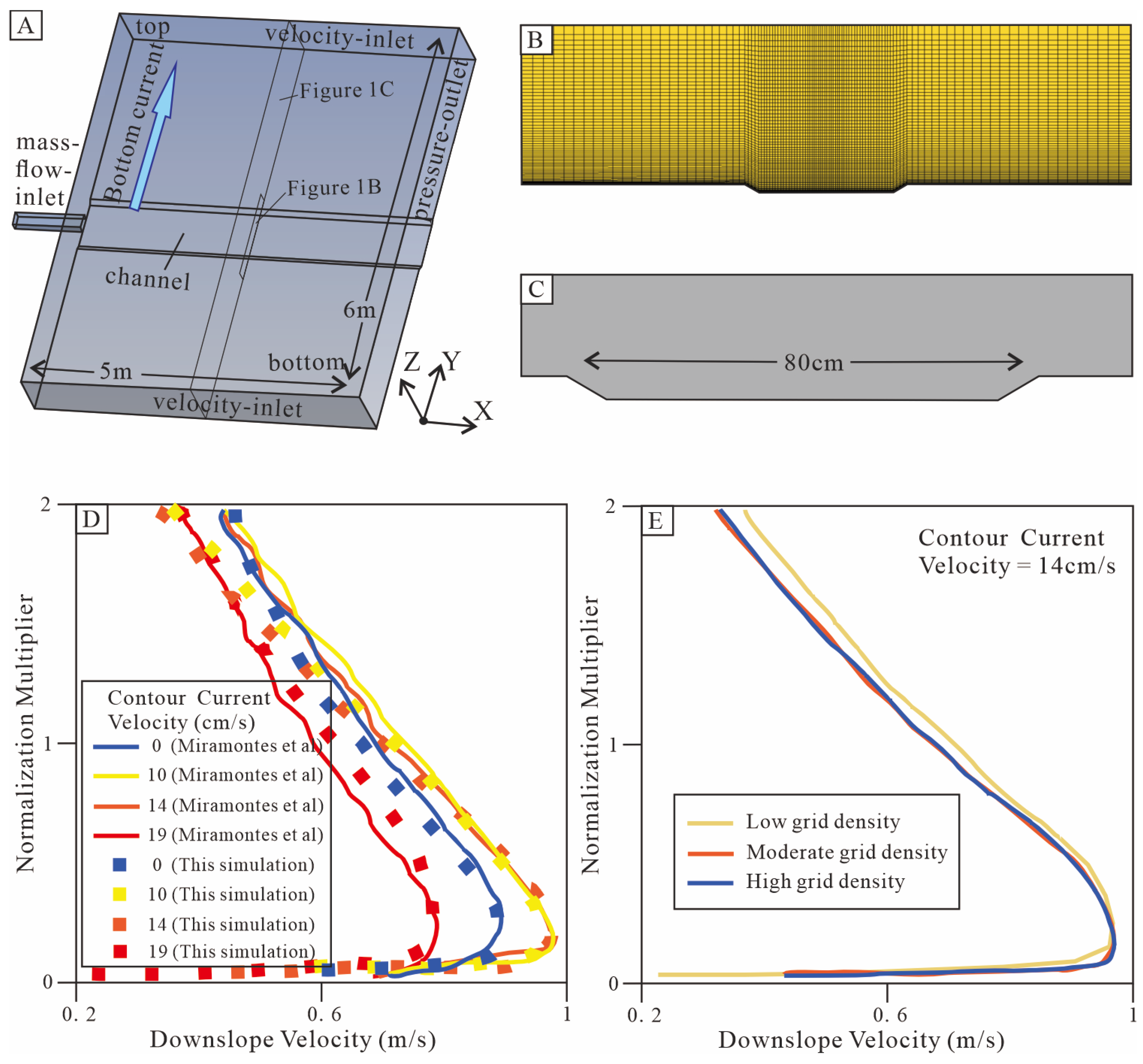
Figure 1. (A) Schematic diagram of the modeling. (B) A grid cross-section in the numerical simulation. (C) Channel cross-sectional profiles applied in the computational model. (D) Model validation between the flume experiments conducted by Miramontes et al. (2020) [28]. (E) Grid independence. The section locations for both (B,C) are indicated in (A).
Jmse 14 00152 g001
Figure 2. (A) Froude number and (B) turbulent shear velocity distributions along the channel cross-section (cross-stream direction), with 0 m representing the channel center.
Jmse 14 00152 g002
Figure 3. Down-stream velocity for different width-to-depth ratios. (A) The maximum flow velocity within the channel reaches 0.5 m/s. (B) The maximum flow velocity within the channel is approximately 0.45 m/s. (C) The maximum flow velocity within the channel is around 0.35 m/s. (D) The maximum flow velocity within the channel is about 0.4 m/s. (E) The maximum flow velocity within the channel is about 0.4 m/s. (F) The maximum flow velocity within the channel is approximately 0.3 m/s. (G) The maximum flow velocity within the channel is around 0.3 m/s. The location of the profiles is indicated in Figure 1C.
Jmse 14 00152 g003
Figure 4. Down-stream velocity at the (A) upstream, (B) midstream, and (C) downstream locations along the channel axis. Since the simulation cases have different channel depths, the depth is normalized to facilitate comparison across cases with varying width-to-depth ratios.
Jmse 14 00152 g004
Figure 5. Cross-stream velocity and velocity vectors for different width-to-depth ratios. (A) Flow field within a channel with a width-to-depth ratio of 5 without a bottom current. (BH) Flow fields within channels with width-to-depth ratios increasing from 5 to 40 when a bottom current is present. The red arrows indicate the identified location and direction of the secondary flow. A secondary flow pointing upstream relative to the bottom current is present on the upstream side. The location of the profiles is indicated in Figure 1C.
Jmse 14 00152 g005
Figure 6. Cross-stream velocity at the (A) upstream, (B) midstream, and (C) downstream locations along the channel axis. Since the simulation cases involve different channel depths, the depth is normalized to facilitate comparison across cases with varying width-to-depth ratios. The dashed line in the figure represents the channel’s top boundary, with the area below it indicating the channel interior.
Jmse 14 00152 g006
Figure 7. (AG) Map view of planform concentration (volumetric percentage) of fine-grained material within each model as the width-to-depth ratio increases from 5 to 40. Darker shades of yellow indicate higher sediment concentrations. For each planform concentration map, the overspill distance is measured as the distance from the channel side to the farthest point where sediment concentration is non-zero in the cross-stream direction. The dashed line in the figure denotes the farthest point where sediment concentration is non-zero in the cross-stream direction.
Jmse 14 00152 g007
Figure 8. Cross-sectional concentration (volumetric percentage) of fine-grained material. In cross profiles (AD), the solid red lines and dashed red lines represent the inclination comparison between the depositional concentration contours (solid lines) and the horizontal reference lines (dashed lines). (AC) When the width-to-depth ratio is less than 10, the sediment concentration contours show a pronounced inclination. (D) As the width-to-depth ratio reaches or exceeds 15, the sediment concentration contours become relatively horizontal. In cross profiles (EG), the black dashed lines outline the overspill extent of sediment, and the vertical distance from the highest point of the black dashed line to the model bottom was measured to indicate the overspill height. The location of the cross-section profile is indicated in Figure 7 and corresponds to the position shown in Figure 1C. Darker shades of yellow indicate higher sediment concentrations.
Jmse 14 00152 g008
Figure 9. (A) The average overspill fluid density increases with the width-to-depth ratio. (BD) Cross-stream distribution of fluid density within the channel at heights of 1.5, 1, and 0.5 times the channel depth, respectively. Channels with larger width-to-depth ratios exhibit greater overspill heights. (E) Comparison of fluid density on both sides of the channel for different width-to-depth ratios. As the width-to-depth ratio increases, the near-bed density distribution shifts from being higher on the left side (red line) to being higher on the right side (blue line). The locations of the measurement lines for Figure 9B–D are shown in Figure 1B.
Jmse 14 00152 g009
Figure 10. The impact of different channel confinements on channel migration patterns. (A) The channel exhibits negligible migration with very strong confinement. (B) The channel migrates downstream with moderate confinement. (C) The channel migrates upstream with weak confinement. The black arrows in the figure represent the direction and location of the flow field transporting sediment within the channel. The red arrows represent the general downstream drift of suspended sediment relative to the bottom current. The green arrows indicate the deflection direction of near-seabed sediment, which controls the potential trend of lateral sediment accumulation. The black dashed lines represent the possible channel after migration.
Jmse 14 00152 g010
Table 1. Tabulations of architectural parameters of unidirectional migrating channels along global continental margins examples.
SchemeWidth/kmDepth/mW/DReference
Negligible migration towards the bottom current
Pacific margin of the Antarctic Peninsula5.535101.57[3,14]
Downstream migration towards the bottom current
Pearl River Mouth Basin1.36101.2513.43[10]
Mauritanian Basin418521.62[16]
Lower Congo Basin3.3213624.44[7]
Upstream migration towards the bottom current
Tanzanian margin1.756029.17[20]
Mozambique margin1.644536.44[12]
Nova Scotia margin3.59038.89[5]
Table 2. Parameters and boundary conditions of the simulation.
ParametersValues
Model length × width/m5 × 6
Model depth/m0.82–0.96
Channel width/m0.8
Channel side wall angle/°30
Environmental fluid density/kg/m31025
Grain density/kg/m32650
Grain volume fraction0.02
Coarse-to-fine grain ratio1:1
Coarse grain size/m0.00006
Fine grain size/m0.00001
Turbidity current velocity/kg/s9
Bottom current velocity/m/s0.1
Time step/s0.0005–0.0001
Maximum iterations20
Table 3. List of numerical simulations, boundary conditions and flow scales.
Case1234567
D (cm)161085.33432
W/D581015202740
U (m)0.20970.21230.20960.21430.25540.21890.2610
h (m)0.19620.14690.14290.10160.14040.11620.1573
Fr1.201.421.411.711.731.631.67
Re43,38533,07831,57622,96137,80526,82743,286
ρ 0 897.651078.061079.991341.451440.761514.671588.89
u * (m/s)0.01490.01330.01450.01240.01700.01180.0188
Note. D—Channel depth, W/D—Width-depth ratio, ρ 0 —Average density of overbank fluid.
Table 4. Number of grids corresponding to different grid densities.
Grid DensitiesNumber of Grids
Low1,185,383
Moderate1,818,984
High2,738,178
Disclaimer/Publisher’s Note: The statements, opinions and data contained in all publications are solely those of the individual author(s) and contributor(s) and not of MDPI and/or the editor(s). MDPI and/or the editor(s) disclaim responsibility for any injury to people or property resulting from any ideas, methods, instructions or products referred to in the content.