Article

Machine Learning-Based Prediction of Maximum Stress in Observation Windows of HOV

1
National Deep Sea Center, Qingdao 266237, China
2
College of Ocean Science and Engineering, Shandong University of Science and Technology, Qingdao 266590, China
3
Yantai Graduate School, Harbin Engineering University, Yantai 264010, China
*
Author to whom correspondence should be addressed.
J. Mar. Sci. Eng. 2026, 14(2), 151; https://doi.org/10.3390/jmse14020151 (registering DOI)
Submission received: 15 December 2025 / Revised: 7 January 2026 / Accepted: 8 January 2026 / Published: 10 January 2026
(This article belongs to the Section Ocean Engineering)

Abstract

With advances in deep-sea exploration technologies, utilizing human-occupied vehicles (HOV) in marine science has become widespread. The observation window is a critical component, as its structural strength affects submersible safety and performance. Under load, it experiences stress concentration, deformation, cracking, and catastrophic failure. The observation window will experience different stress distributions in high-pressure environments. The maximum principal stress is the most significant phenomenon that determines the most likely failure of materials in windows of HOV. This study proposes an artificial intelligence-based method to predict the maximum principal stress of observation windows in HOV for rapid safety assessment. Samples were designed, while strain data with corresponding maximum principal stress values were collected under different loading conditions. Three machine learning algorithms—transformer–CNN-BiLSTM, CNN-LSTM, and Gaussian process regression (GP)—were employed for analysis. Results show that the transformer–CNN-BiLSTM model achieved the highest accuracy, particularly at the point exhibiting the maximum the principal stress value. Evaluation metrics, including mean squared error (MSE), mean absolute error (MAE), and root squared residual (RSR), confirmed its superior performance. The proposed hybrid model incorporates a positional encoding layer to enrich input data with locational information and combines the strengths of bidirectional long short-term memory (LSTM), one-dimensional CNN, and transformer–CNN-BiLSTM encoders. This approach effectively captures local and global stress features, offering a reliable predictive tool for health monitoring of submersible observation windows.

1. Introduction

The observation window is a critical component of human-occupied vehicles (HOV) and comprises polymethyl methacrylate (PMMA) [1]. During descent, it experiences stress accumulation owing to external loads [2,3]. In stress prediction for observation windows under loading conditions, the maximum principal stress is crucial. When the maximum principal stress exceeds the tensile or compressive strength of the material, failure may occur via either tensile or compressive modes. Hence, ensuring that the observation window withstands maximum principal stress under extreme external pressures is crucial for maintaining structural integrity and safety.
Conventional stress analysis methods primarily rely on numerical simulations, such as finite element analysis (FEA) [4]. Wang et al. [5] conducted a systematic investigation into the mechanical response characteristics of PMMA (Polymethyl Methacrylate), a commonly used material for observation windows, in high-pressure environments. The study utilized a linear elastic model to perform initial finite element analysis in ABAQUS. Subsequently, quasi-static loading and unloading experiments were carried out within a high-pressure chamber to capture strain and central displacement data at key locations. A comparison with the simulation results revealed significant discrepancies during high-pressure phases. Further analysis indicated that an increase in temperature (28–32 °C) affects the elastic modulus of PMMA, leading to a reduction of approximately 10%. The findings suggest that within the low-pressure range of up to 80 MPa, the linear elastic model demonstrates good consistency with experimental results, serving as an effective method for simplified design. Zhou et al. [6] exhibited the creep behavior of thick PMMA materials submerged in liquid under eight different stress levels. Arnold et al. [7] proposed a predictive model for the mechanical behavior of PMMA, which aligns well with experimental outcomes. Additionally, Pranesh et al. [8] examined various design strategies for observation windows to mitigate internal stress, achieving a significant reduction in corner stress through the selection of optimal radius dimensions.
Although these approaches accurately predict the stress distribution to a certain extent, they are computationally expensive, time-consuming, and less adaptable to complex loading conditions. With the rapid advancement of artificial intelligence, data-driven methods have provided a new direction for stress prediction [9]. Deep learning models [10] have demonstrated considerable potential in predicting stress in complex systems owing to their robust feature extraction capabilities and high predictive accuracy. Enjamamul Hoq et al. [11] developed and evaluated two data-driven approaches for predicting full-field stress responses. The first combines a reduced-order model using proper orthogonal decomposition (POD) with conventional machine learning algorithms such as k-nearest neighbors, random forests, and artificial neural networks to predict full-field responses from reduced POD coefficients. The second employs a ResNet-based convolutional neural network (CNN) and an improved conditional generative adversarial network (cGAN). Swischuk et al. [12] utilized POD to reduce the dimensionality of high-fidelity field data and applied artificial neural networks, k-nearest neighbors, decision trees, and multivariate polynomial regression approaches to predict the pressure or strain fields in two engineering cases. Chinesta et al. [13] emphasized that model order reduction (MOR) techniques considerably enhance the efficiency of full-field response prediction involving numerous output variables. In MOR, high-fidelity data are projected into a lower-dimensional subspace, thereby reducing computational complexity and enabling more efficient learning and training during the online stages.
Computer vision-based deep learning methods can extract meaningful model features, enabling accurate field predictions across diverse applications. Tripathy et al. [14] employed deep learning for image enhancement and correction, while Yu et al. [15] focused on mesh quality enhancement. Leger et al. [16] utilized real-time fault object recognition for quality control, while Bagave et al. [17] applied these techniques for predictive maintenance and machine failure forecasting. In recent years, the application of convolutional neural networks (CNNs) in engineering problems has grown considerably. Lee and You [18] applied CNNs to a fluid flow analysis, while Li et al. [19] used them for heat transfer studies. Abueidda et al. [20] utilized CNNs in topology optimization and Donegan et al. [21] applied them to modeling material plasticity and fracture. Zhang et al. [22] used CNNs for seismic response analysis. Nie et al. [23] developed two CNN architectures, a convolutional autoencoder and ResNet-based model, to predict stress fields in a cantilever structure made of homogeneous material. Herriott and Spear [24] utilized ridge regression, gradient boosting, and CNNs to predict the effective yield strength of additively manufactured metals, demonstrating that CNNs outperformed conventional methods in learning high-level features directly from image data.
The generative adversarial network (GAN) framework proposed by Goodfellow et al. [25] has been widely applied in image-to-image translation, high-resolution image synthesis, and video sequence prediction. GANs comprise two deep neural networks: a generator and discriminator, trained adversarially to produce data aligned with the original distribution. Chen and Gu [26] introduced a generative deep neural network for robust inverse design modeling to identify candidate materials. Ni and Gao [27] utilized cGAN to predict modulus distribution by constructing a representative shear modulus sampling space. Jiang et al. [28] employed an image-to-image translation-based cGAN model to design high-quality composite materials with enhanced toughness.
The aforementioned studies show that POD-based conventional machine learning methods and computer vision-oriented deep learning approaches are effective for predicting physical fields. Stress prediction for observation windows involves managing large datasets and high computational complexity, resulting in extended training and prediction times. Conversely, predicting a single metric reduces computational demands and enables more efficient training and prediction. This targeted approach enables rapid identification of critical stress states, facilitating structural assessment and reinforcement. To achieve this, a model combining Transformer–CNN-BiLSTM (generally used in natural language processing) with long short-term memory networks was developed and compared to conventional machine learning methods—Gaussian process regression and CNN-LSTM models. In this architecture, one-dimensional convolutional layers extract local features from the input data, capturing short-term dependencies [29], while the bidirectional LSTM component models long-term dependencies. Additionally, the multihead attention mechanism in the transformer encoder captures global contextual information, thereby enhancing the ability of the model to learn complex temporal patterns. As the transformer–CNN-BiLSTM encoder lacks inherent sequential awareness, a positional encoding layer is introduced to embed positional information, enabling recognition of relative relationships among sequence elements. Applying transformer–CNN-BiLSTM in predicting the maximum principal stress of observation windows in HOV has not yet been explored, highlighting its potential for future research.
The remainder of this paper is organized as follows: Section 2 presents the data acquisition process, including experiments subjecting the observation window to pressures of up to 80 MP; in addition, Section 2 introduces and discusses three prediction models for maximum principal stress: transformer–CNN-BiLSTM, CNN-LSTM, and GP. Section 3 provides an in-depth analysis of the results, while Section 4 presents a comparative evaluation of the model performance. Section 5 summarizes the findings and outlines directions for future research.

2. Materials and Method

2.1. Data Source

The dataset utilized in this study was obtained from experiments conducted on observation window samples (Jiangsu Tie Mao Technology Co., Ltd., Nantong, China) of HOV within a high-pressure test chamber. These samples were designed and manufactured to replicate actual operational conditions under different load and environmental conditions. The observation window design followed the ASME PVHO-1 standard and analyzed data in UEIlogger (Version 3.0.0). For clarity, the larger surface of the sample is referred to as the “front,” while the smaller surface is referred to as the “back,” corresponding with the light direction. The structure is illustrated in Figure 1, where the back diameter Φ1 = 37.6 mm, the front Φ2 = 153.2 mm (along the direction of light transmission), and height H = 60.4 mm. The front features a chamfer angle of R = 115° and cone angle of α = 90°. The mechanical parameters of the PMMA sample are presented in Table 1.
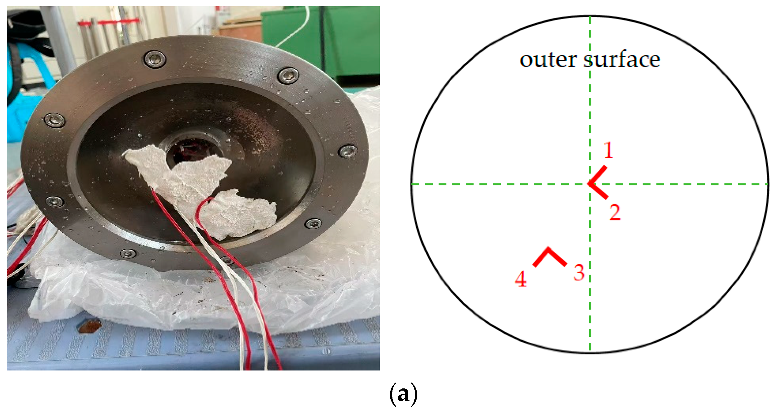
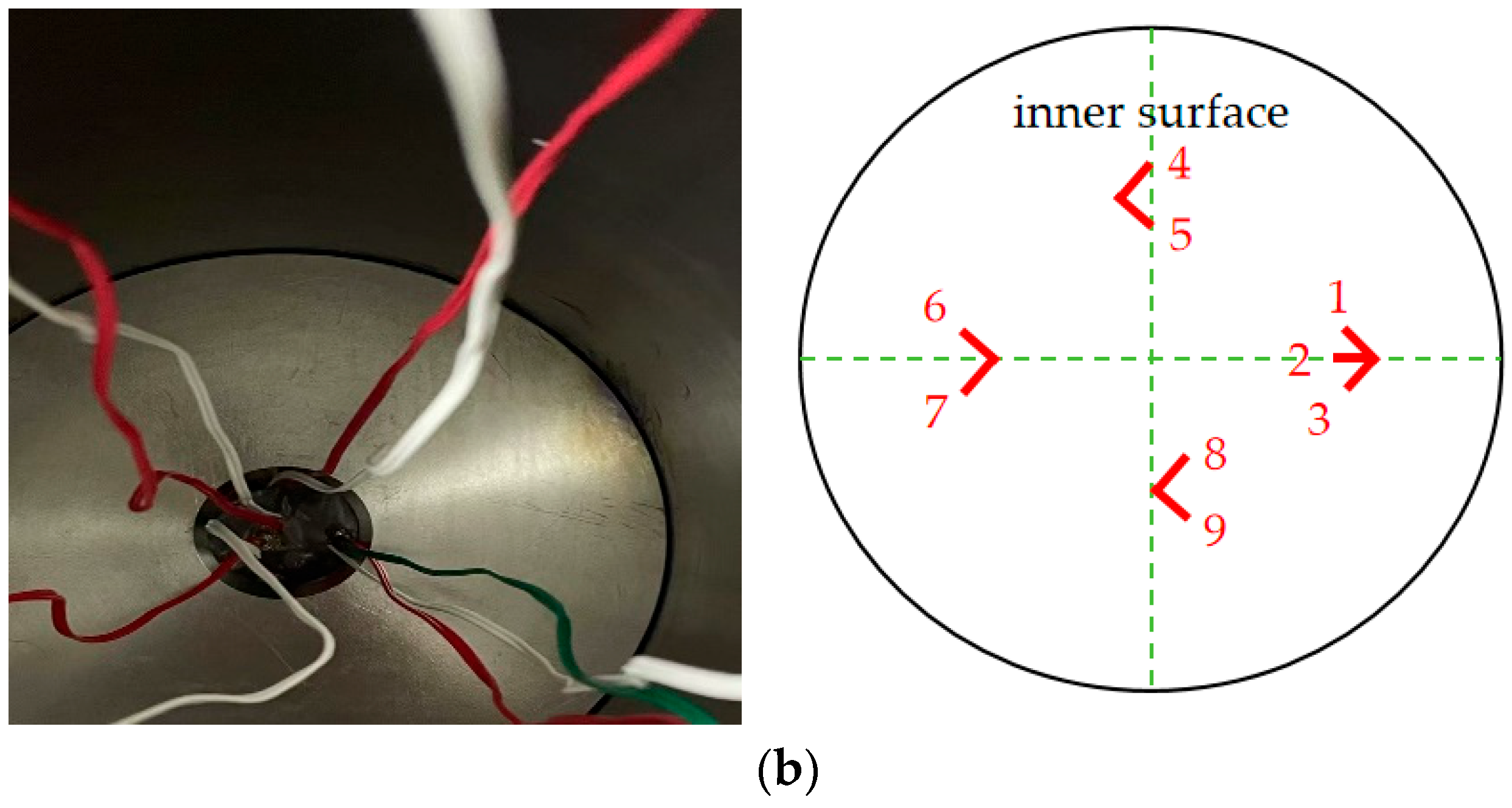
The high-pressure test chamber, located at the national deep sea center, is a specialized facility designed to simulate deep-sea environments and can withstand pressures up to 115 MPa. In this experiment, six strain gauges were strategically installed in the observation window area of the chamber to monitor the strain at different locations, thereby assessing stress distribution and structural integrity under high-pressure conditions. Two bidirectional strain gauges were mounted on the flat exterior surface of the observation window (Figure 2a), while three bidirectional strain gauges were positioned on the flat interior surface. Additionally, a triaxial strain gauge was positioned near the chamfer, 4 mm from the observation window (Figure 2b). This region is crucial owing to stress concentration arising from geometric characteristic, making strain gauge placement critical for accurate monitoring.
To monitor pressure variations within the high-pressure test chamber, high-precision pressure sensors with an accuracy of 0.1 MPa were integrated into the experimental setup. These sensors recorded real-time pressure changes on the observation window surface, as illustrated in Figure 3. Coupled with strain data, the recorded pressure values provided high-quality input variables for subsequent deep learning models, forming a comprehensive dataset. A total of 13,149 sets were collected, each comprising time-dependent strain values from five strain gauges in multiple directions and corresponding load data over time. The experiment was conducted in three distinct phases: (1) pressurization to 80 MPa, (2) holding at 80 MPa, and (3) depressurization to 0 MPa. The entire process was repeated twice, with an extended holding period during the second cycle to enable detailed observation of the strain behavior across different gauges under varying load conditions, as shown in Figure 4. Herein, channels 1–3 represent strain values from the internal triaxial strain gauges (referring to channels 1 to 3 shown in Figure 2a), 4–9 the internal bidirectional gauges (referring to channels 4 to 9 shown in Figure 2b), and 10–12 relate to the external bidirectional gauges (referring to channels 1 to 3 shown in Figure 2b). During the experiment, Channel 13 was damaged and consequently did not yield any data. The strain curves exhibit distinct rising and falling patterns corresponding with the loading and unloading phases. During the pressurization initial phase, strain values gradually increased, indicating deformation of the observation window under applied load.
Towards the end of the curves, the strain values start recovering, indicating that the observation window deformation gradually returns to its original state after unloading. Around the data midpoint (approximately 2000 s), the curve reaches its maximum strain value (including negative values), corresponding to the peak loading phase during this period. Channel 3 consistently exhibits higher strain values throughout the loading and unloading processes, which can be attributed to its location—the internal triaxial strain gauge positioned near the stress concentration region of the observation window—suggesting it experiences greater load effects. Channels 11 and 12 exhibit more pronounced fluctuations in strain values owing to their external placement, resulting in considerable variability around the peak and trough values.
In this experiment, a quarter-bridge configuration was utilized for the strain gauges during the strain data acquisition. This configuration introduces nonlinear errors into the measured strain values. To address this issue, the nonlinear correction formula expressed in Equation (1) was applied to obtain the true strain value, denoted as ε .
ε = ε 0 1 ε 0
where ε 0 represents the measured strain values obtained during the experiment.
Given the short duration of the descent and ascent phases, creep effects were not considered. The strain data collected from the triaxial direction on the internal surface of the observation window were utilized to calculate the maximum principal stress, as expressed Equation (2). This approach provides comprehensive and accurate data support for subsequent stress predictions in machine learning models.
σ max = E 2 1 v 2 ( 1 + v ) ε a + ε c + ( 1 v ) × 2 ε a ε b 2 + ε b ε c 2
Under the condition of plane strain, σ max refers to the magnitude, where E and v represent the elastic modulus and Poisson’s ratio of the experimental materials, respectively, with specific values detailed in Table 1. Additionally, ε a , ε b and ε c correspond to the strain measurements taken in three different directions from the strain gauges.
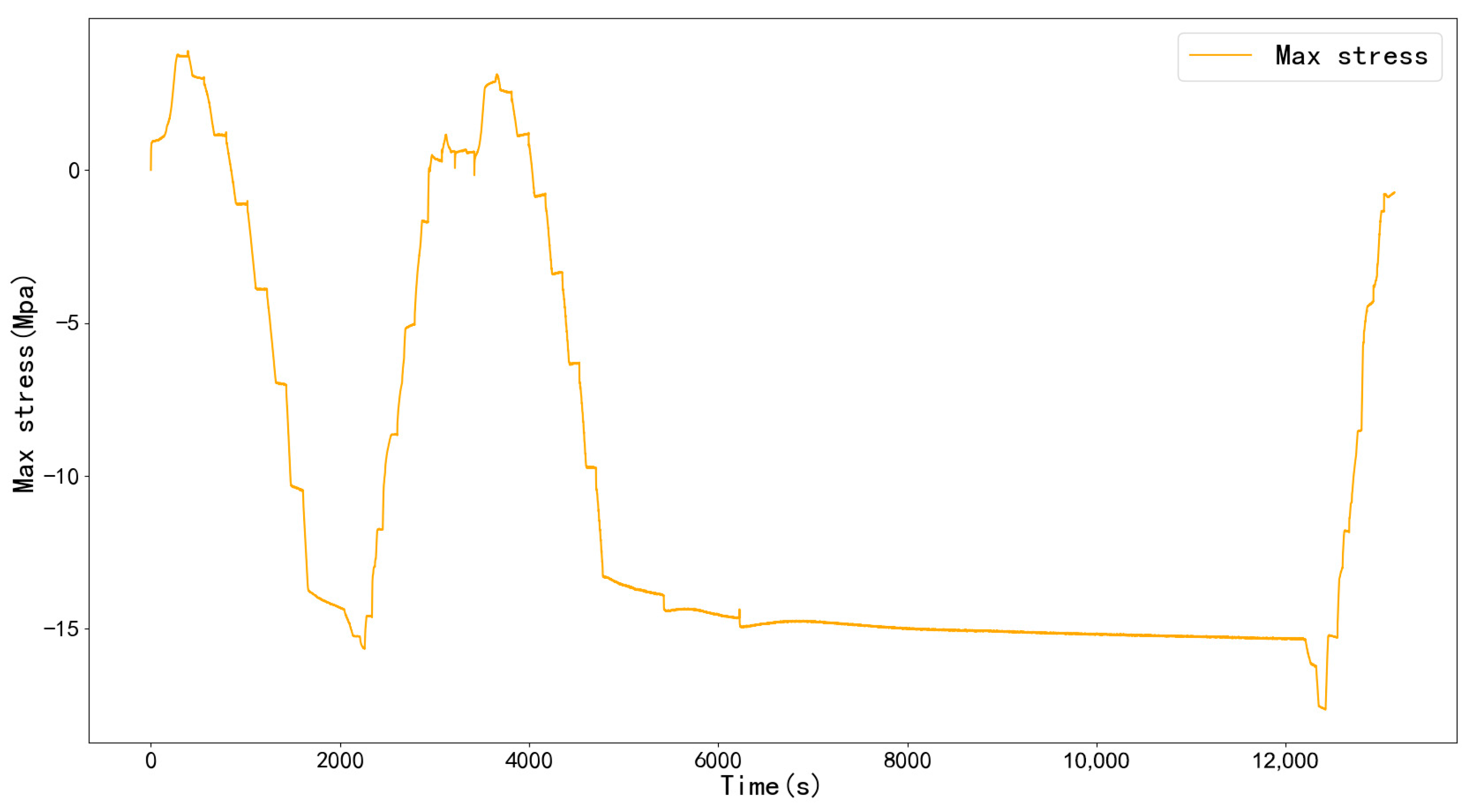
The variation in the maximum principal stress over time is shown in Figure 5. During the initial loading phase, the maximum principal stress increased rapidly and reached a local peak, indicating the formation of a distinct stress distribution within the structure as external pressure rose. Simultaneously, the strain curves from different channels exhibited rapid changes, particularly in Channel 3, where the strain values considerably increased. The strain gauge data confirmed localized strain concentrations, corresponding with the rapid increase in maximum principal stress. This correlation highlights the occurrence of pronounced stress concentration during the initial loading phase. During the holding pressure stage, the maximum principal stress stabilized with minor fluctuations. These fluctuations may be attributed to the material creep behavior or adjustments in contact conditions. During the unloading phase, the maximum principal stress decreases rapidly, returning to stress levels observed prior to unloading.
The strain data for the observation window at different loading pressures were obtained using experimental measurements. The results show that the distribution and concentration of maximum principal stress during the high-pressure loading considerably affect structural safety. These analyses provide a theoretical basis for maximum principal stress prediction using machine learning methods, enabling more efficient assessment of mechanical performance and supporting the optimization of the observation window design. The strain gauge data and maximum principal stress data acquired from the experiment served as training and validation datasets for the deep learning model. The applied load, used as a direct control variable, was varied stepwise to provide time-series input features for the model, while the maximum principal stress—a key indicator of structural safety—was designated as the target output.
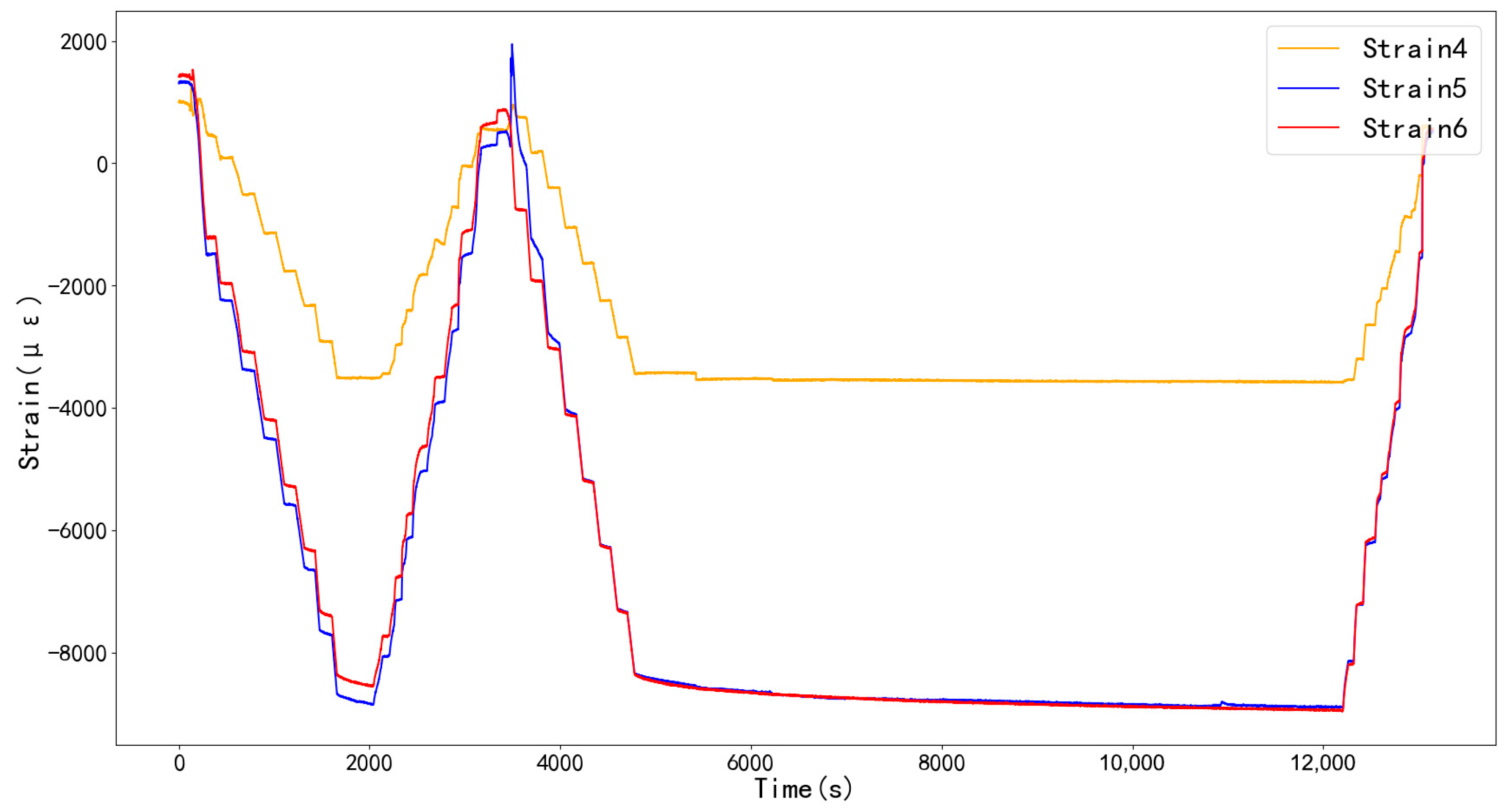
The dataset comprised time steps of the external load and strain data from two external strain gauges (measured in two directions), as shown in Figure 6, coupled with the maximum principal stress values obtained from the internal strain gauges (measured in three directions). Herein, the external load time steps and strain data were used as input features, while the maximum principal stress values served as the model output.
To simplify the model, an alternative dataset was constructed using the external load and strain data as inputs, with the maximum principal stress remaining as the output. In this dataset, Strain4 represents the axial strain values from the two external strain gauges, while Strain5 and Strain6 correspond with the axial and transverse strains, respectively, from another set of external gauges. This approach enables the assessment of how different feature combinations influence the predictive performance of the maximum principal stress.
To quantitatively assess the correlation between the target variable (maximum principal stress values) and environmental predictors (input features), the Pearson correlation coefficient was calculated, as illustrated in Figure 7. This analysis examines the linear correlation degree between the input features and principal stress values. The correlation coefficient is expressed as follows:
r = i = 1 n x i x ¯ y i y ¯ i = 1 n 1 x i x ¯ 2 i = 1 n 1 y i y ¯ 2
where x i and y i represent the observed values for each paired sample, x ¯ and y ¯ their respective means, and n the number of samples.
As illustrated in the figure, red denotes positive correlation ( r > 0) and blue negative correlation ( r < 0). The color intensity reflects the correlation magnitude, with darker tones indicating stronger relationships, while bubble size corresponds proportionally to the absolute correlation values. To enhance model training stability and prediction accuracy, data normalization was applied as follows:
Z = X X min X max X min
where X represents the original data; X m i n and X m a x its minimum and maximum, respectively; and Z the normalized data. The dataset was then divided into training and testing sets. Due to the nature of the experimental data as time series, this study opted for a time block partitioning approach, with 80% used for training and 20% for evaluating generalization performance. This method ensures the continuity of the time series within both the training and testing datasets.

2.2. Machine Learning Algorithms

2.2.1. Gaussian Process Regression

Rasmussen and Williams [30] considerably advanced GP application in machine learning. A GP can be regarded as a collection of random variables, any finite subset of which follows a joint Gaussian distribution. It defines a distribution over functions characterized by this joint distribution. To predict the maximum principal stress of the observation window, this study employs GP to model the objective function. Assuming that the function f(x) is a random process, it follows a Gaussian distribution for any input x as follows:
f ( x ) G P m ( x ) , k x , x
where m(x) represents the mean function and k(x,x′) the kernel function. The mean function is generally set to zero, while the kernel quantifies the similarity between input data points. In this study, the radial basis function (RBF) kernel, also known as the Gaussian kernel, is used because it effectively captures the similarity between features such as pressure and external strain data. Its parameters are optimized using the training dataset as follows:
K R B F x , x = exp x x 2 2 σ 2
where | | x x | | 2 represents the squared Euclidean distance between input points x and x′ and σ a hyperparameter controlling the function smoothness. The RBF kernel evaluates feature similarity and is optimized using the training data.
The model is then trained to learn the mapping input features—pressure and external strain data—and the output (MPA) while simultaneously optimizing the kernel parameters. The training process is conducted by maximizing the log-likelihood function as follows:
log p ( y X ) = 1 2 y T K 1 y 1 2 log | K | n 2 log 2 π
where X represents the input feature matrix, y the target value vector, K the kernel matrix, and n the number of samples.
After training, the model was used to predict the distribution of the target value f for a new test point X expressed as follows:
p f X , X , y = N f ¯ , V a r f
where the predictive mean f ̄ and variance V a r f are expressed as follows:
f ¯ = K X , X K ( X , X ) 1 y V a r f = K X , X K X , X K ( X , X ) 1 K X , X
where K X , X denotes the kernel matrix between test and training points and K X , X the matrix among training points.
The model parameters were set as follows: The constant kernel had an initial value of 1.0 (optimization range: 1 × 10⁻³, 1 × 10³) and RBF Kernel an initial length scale of 10 (range: 1 × 10⁻², 1 × 10². The final kernel was denoted as C d R B F . To avoid local optima, the number of optimization restarts was set to 10, while the regularization strength of 1 × 10⁻¹⁰ was applied to enhance numerical stability.

2.2.2. CNN-LSTM

The CNN-LSTM model is a hybrid neural network architecture that combines the advantages of CNN and LSTM networks. As demonstrated by Masood and Ahmad [31], this architecture is effective for managing computer vision and time-series data. The CNN component extracts local features from the input data, while the LSTM component captures the temporal dependencies inherent in sequential data. To predict the maximum principal stress of the observation window, local features were first extracted from the time-step and external strain data using the CNN model, which then served as inputs for the LSTM model for prediction.
CNNs are deep learning models well-suited for processing grid-like data such as images or time series. Deep CNNs comprise multiple layers, including convolutional, pooling, and fully connected layers, enabling efficient computation and multilevel feature extraction. The convolutional layers generate feature maps by performing convolutional operations that combine the input values with kernel weights and biases [32]. Each convolutional kernel comprises parameterized weight matrices designed to capture local spatial and temporal patterns within the input data.
To reduce the number of model parameters while preserving key features, the pooling layers perform dimensionality reduction on the outputs of the convolutional layers. These layers compress data by computing statistical measures—such as maximum or average values—over local regions, thereby enhancing computational efficiency and reducing storage requirements. To connect the multi-dimensional feature maps from the convolutional layers to the predicted outcomes, a flattening layer is introduced between the convolutional and fully connected layers, transforming the multi-dimensional data into a one-dimensional vector. The fully connected layer then integrates these features to complete the mapping from the input to the output. Figure 8 shows the CNN process, wherein a convolutional kernel size of 2 is utilized.
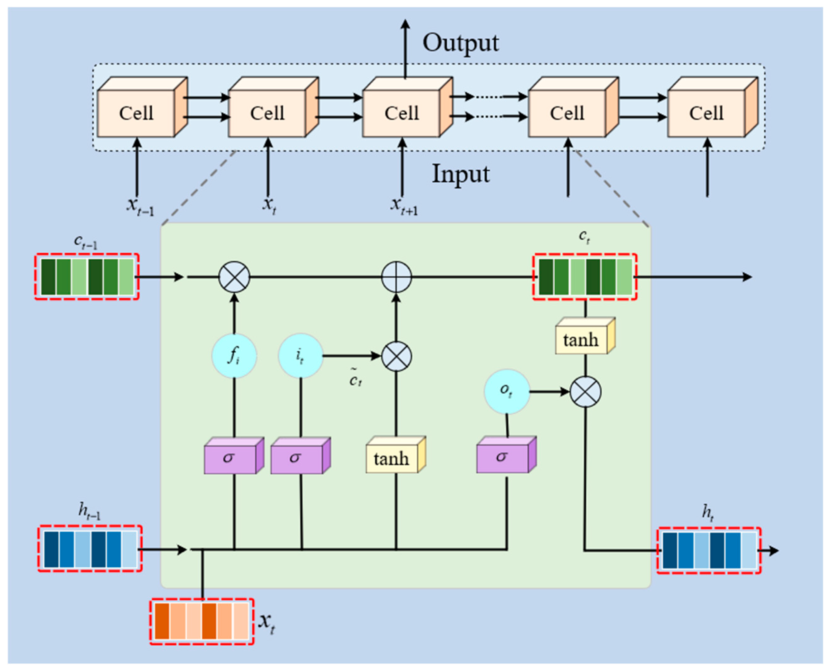
The structure of the CNN-LSTM model is shown in Figure 9. The CNN component includes an input layer, convolutional layers, pooling layers, and a flattening layer. The output of the CNN serves as the input to the LSTM, where 1D convolutional and pooling layers extract spatial features from the input data. The flattening layer bridges the CNN and LSTM components by converting the extracted features into a one-dimensional array suitable for sequential processing. The LSTM output layer then generates the predicted maximum principal stress, as shown in Figure 10. In this study, three sets of 1D convolution and pooling operations were implemented; subsequently, the flattening operation was carried out on the two LSTM layers and the output layer to facilitate output prediction. Each LSTM layer incorporated a dropout layer with a dropout rate of 0.5 to reduce overfitting. The hyperparameters were configured as follows: learning = 0.001, number of neurons between convolutional and pooling layers = 64, and both convolutional kernel and pooling sizes = 1. Each LSTM layer comprised 100 neurons, while the ReLU activation function was employed. To prevent gradient explosion during training, gradient clipping was applied beforehand, limiting the gradient magnitude to a maximum value of 1 before optimization.
This study leveraged the local feature extraction capability of CNNs to identify key patterns from time-step and strain data. The convolutional layers detected local features, while pooling layers reduced the dimensionality of the extracted information. The fully connected layers mapped these features to predict maximum principal stress values. This structure effectively captured local and global patterns in the data, providing a scientific basis for accurate stress prediction under high-pressure conditions.

2.2.3. Transformer-CNN-BiLSTM

The Transformer model was introduced by Vaswani et al. [33]. Pre-trained transformer-based models such as BERT and GPT have considerably advanced deep learning across domains including natural language processing, computer vision, and time series analysis. In the transformer–CNN-BiLSTM architecture, raw data such as pressure and strain features are first processed by a CNN to extract local patterns and capture short-term dependencies. These features are then passed to the LSTM layer, which captures dynamic relationships and produces a hidden state sequence or global temporal features. Unlike conventional CNN-LSTM models, this architecture incorporates a transformer encoder that utilizes the Query–Key–Value (QKV) attention mechanism and multi-head attention to model global interactions among input features. The encoder further integrates positional encoding to embed temporal and spatial dependencies, enabling richer and more comprehensive feature representation.
The decoder module of the transformer–CNN-BiLSTM model employs masked multi-head attention together with historical predictions to ensure temporal consistency in sequential outputs. Unlike conventional models that rely solely on the recursive nature of LSTM for time-series modeling, the decoder enables parallel input processing, thereby enhancing sequence generation efficiency. The decoded features are then mapped to target stress values through fully connected layers, forming an integrated framework that transitions from local features to global patterns and from short-term dynamics to long-term dependencies.
The primary advancements of the transformer–CNN–BiLSTM model over the CNN-LSTM model include the integration of transformer encoder and decoder modules, which enhance global interaction capturing and reduce dependence on extended sequences. The QKV attention mechanism strengthens relationships among features, particularly for modeling long-range dependencies, while the masked multi-head attention enables parallel computation, thereby increasing efficiency and addressing the limitations of recursive LSTM operations.
The model structure is shown in Figure 11. By integrating local feature extraction from CNNs, temporal dynamic modeling from LSTMs, and global interaction learning from transformers, this model achieves comprehensive modeling and accurate stress prediction.

3. Results

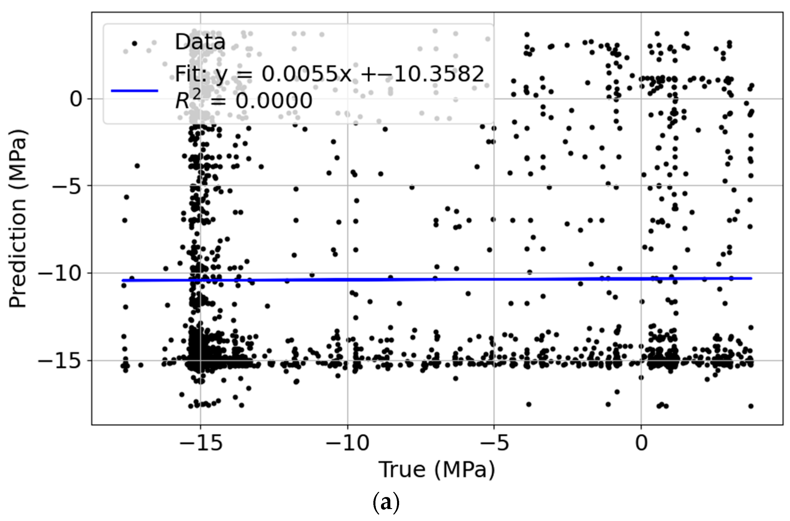
This study provides a detailed analysis of the performance of two datasets in model predictions. The first dataset comprises external load time steps, strain data from two external strain gauges (measured in two directions), and maximum principal stress values derived from internal strain gauges (measured in three directions). In this dataset, the time steps and strain data from the two external gauges are used as input features, while the maximum principal stress values serve as the predicted output for the model. Experimental results indicate that utilizing a dataset with multidimensional features enables the model to more accurately capture the effects of external loads and strain variations on the maximum principal stress, resulting in significantly reduced prediction errors. Furthermore, the model demonstrates strong performance in capturing nonlinear characteristics and temporal dynamics, further validating its applicability in processing complex input data.
In contrast, the second dataset employs simplified features, containing only external load time steps and associated time step characteristics as input, with maximum principal stress values as the predicted output. The experimental findings reveal that, despite the reduction in input dimensionality, the model still achieves high predictive accuracy, particularly within regions of steady load variation, where the prediction errors are minimal. However, due to the simplification of input features, the model displays some limitations in capturing the nonlinear relationships between strain and principal stress, which results in an increased discrepancy between predicted and actual values, especially during periods of rapid load change.
The fitting lines of the three models for the first dataset are shown in Figure 12. The slopes of the fitting lines and R2 values close to 1 in the scatter plots indicate minimal prediction errors.
Figure 13 illustrates the fitting lines of the three models for the second dataset. The fitting performance was considerably affected by the reduction in feature dimensions. Unlike the first dataset, the second dataset included only external load time-steps and time-step characteristics, excluding external strain information. This decrease in feature dimensions increased the learning difficulty for all models, particularly in capturing nonlinear stress variations.
Figure 14 shows the predicted maximum principal stress results for the first dataset. Among the models, the GP model exhibited the highest prediction errors and failed to effectively track actual stress variations. The CNN-LSTM model showed deviations at peak regions, while the transformer–CNN–BiLSTM model achieved the lowest prediction error, demonstrating superior performance. In fitting performance at the peak and trough values, the GP model performed poorly, while the CNN-LSTM model exhibited slight lag and the transformer–CNN–BiLSTM model accurately captured changes at the local extrema.
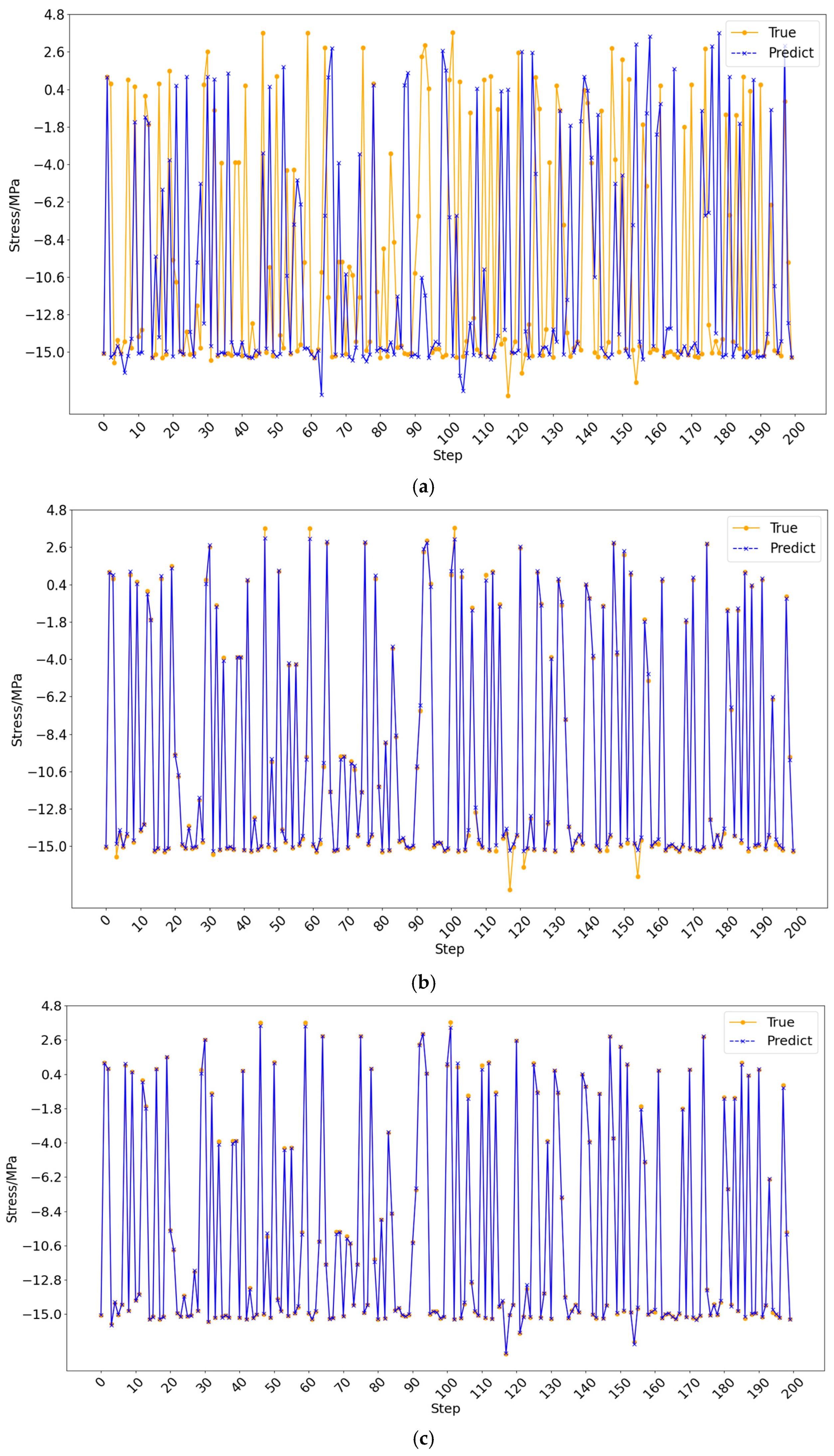
Figure 15 shows the predicted maximum principal stress results for the second dataset. The reduced input features constrained the models to rely on limited information, thereby increasing the demand for generalization. Under these circumstances, the transformer–CNN-BiLSTM model demonstrated the best predictive performance, maintaining strong agreement with the overall trend and minimizing errors in the peak and trough regions.

4. Comparison of Models

Maximum principal stress prediction within the observation window is a regression problem. Evaluating model performance requires assessing the deviation between predicted and actual values and similarity in their distributions. This study employed the mean squared error (MSE), mean absolute error (MAE), and root squared residual (RSR) to quantify discrepancies between true and predicted values across models. These evaluation metrics are expressed as follows:
M S E = 1 n t = 1 N y t y p r e d i c t   2
M A E = 1 n t = 1 N y t y p r e d i c t  
R S R = t = 1 N y t y p r e d i c t   2 t = 1 N y t y a v e r a g e   2
where N represents the number of observations, y t the true value, y p r e d i c t the predicted value, and y a v e r a g e the mean of the true value. Smaller MSE and MAE values indicate better model performance, while an RSR value closer to 0 is preferable.
MSE, MAE, and RSR were employed to compare discrepancies between true and predicted values across models, thereby assessing the performance of deep learning and machine learning models.
For the first dataset, the performance of the three models was evaluated using the aforementioned metrics, and the results are presented in Table 2. The transformer–CNN–BiLSTM model outperformed the other models across all metrics, exhibiting lower values for each indicator and an RSR closer to zero.
On the first dataset, the transformer–CNN-BiLSTM model achieved a 69.03% reduction in MSE, 24.11% in MAE, and 44.3% in RSR compared to the CNN-LSTM model, demonstrating considerable enhancement in capturing global dependencies and sequential features, notably in highly nonlinear and time-dependent data. Further, the CNN-LSTM model outperformed the GP model across all metrics, indicating that combining convolutional neutral networks with LSTM effectively addresses complex stress prediction tasks. Although the GP model can address simpler prediction issues, it exhibits clear limitations in modeling high-dimensional and complex nonlinear tasks. The comparative metrics for the three models are illustrated in Figure 16.
To investigate the variations in the metrics during each training epoch, the changes in the indicators for the first dataset are presented in Figure 17.
To further analyze performance evolution during training, the variations in MSE, MAE, and RSR for the first dataset are shown in Figure 17. As the GP model does not have an iterative training process like deep learning models, it is not possible to conduct an analysis based on the changing trends of training loss and test loss. To compare its prediction performance, this study only evaluates its prediction effect using the slope of the fitted line and the coefficient of determination (R2 value). Only the CNN-LSTM and transformer–CNN–BiLSTM models were compared. The transformer–CNN–BiLSTM model demonstrated a faster convergence rate and lower final values across all indicators than the CNN-LSTM model. These improvements are primarily attributed to the transformer module, whose multi-head attention mechanism captures global dependencies and effectively models complex nonlinear strain–stress relationships. Further, the transformer module enhances multidimensional feature representation and accelerates parameter optimization, resulting in superior predictive performance.
The second dataset was similarly used to evaluate the performance of the three models using MSE, MAE, and RSR, as presented in Table 3.
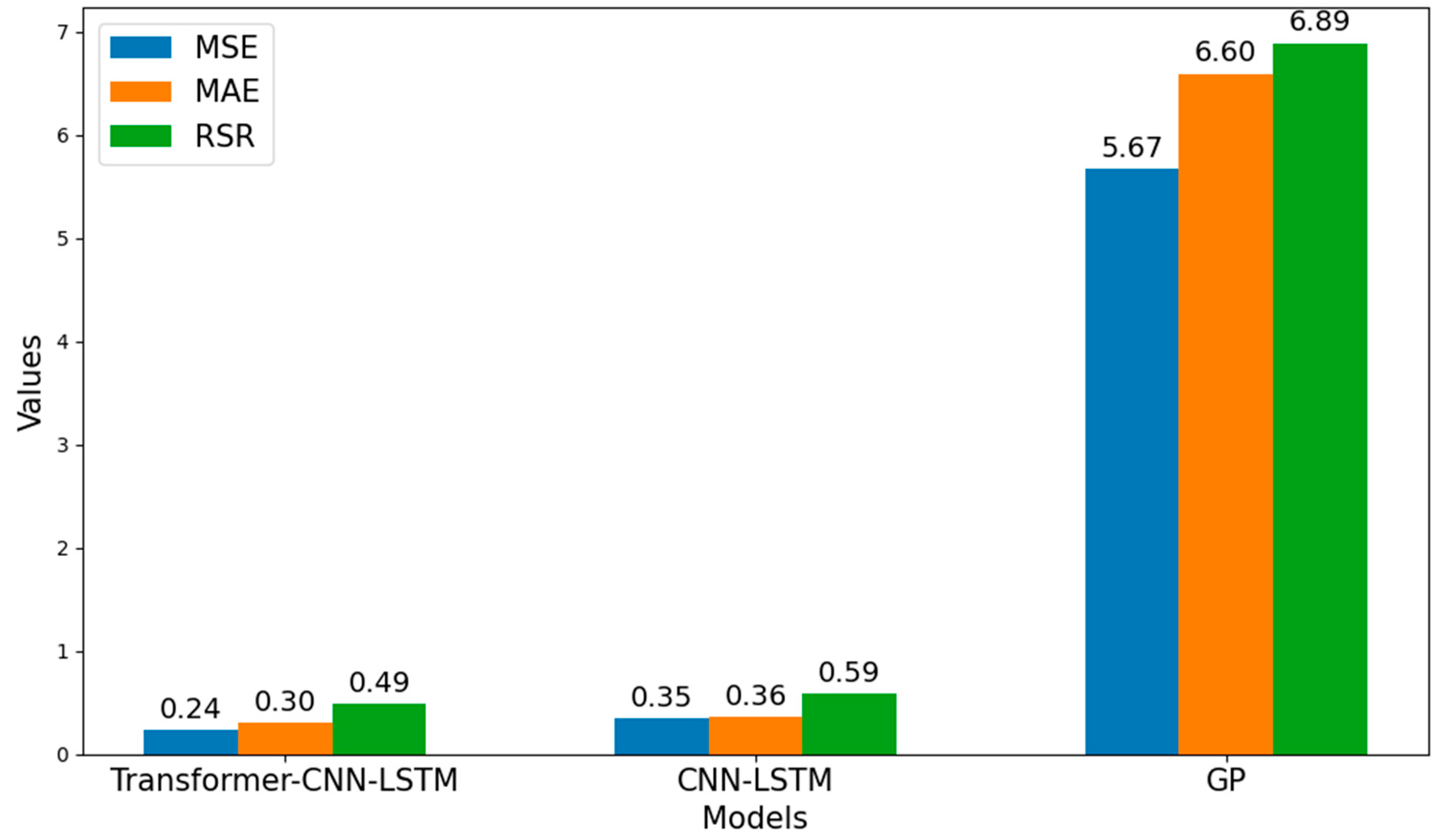
The transformer–CNN–BiLSTM model achieved reductions of 31.1% in MSE, 17.01% in MAE, and 16.98% in RSR compared to the CNN-LSTM model. Additionally, the CNN-LSTM model exhibited considerably lower MSE, MAE, and RSR values than the GP model, confirming its superior ability to model nonlinear stress–strain relationships. The comparative metrics for the three models on the second dataset are shown in Figure 18.
Figure 19 shows the variations in the metrics across training epochs for the second dataset.
The transformer–CNN–BiLSTM model exhibited a rapid decrease in all three metrics during the initial phases, with a notably faster convergence rate than the CNN-LSTM model. After the 20th epoch, the MSE and MAE trends stabilized, indicating improved training consistency. Additionally, the fluctuations in RSR were considerably smaller than those in the CNN-LSTM model.

5. Conclusions

This study addresses maximum principal stress prediction in observation windows by developing a finite element model to verify the equivalence between two- and three-dimensional analyses. Stress concentration regions were identified, while strain gauges were strategically placed nearby to collect experimental data, forming the basis of the machine learning datasets. Three models—GP, CNN-LSTM, and transformer–CNN-BiLSTM—were developed and systematically compared using two distinct datasets.
In the comparative analysis, the transformer–CNN-BiLSTM model outperformed the CNN-LSTM and GP models across all performance metrics (MSE, MAE, and RSR). On the first dataset, it achieved MSE, MAE, and RSR values of 0.0183, 0.0954, and 0.1353, respectively, representing reductions of 69.03%, 24.1%, and 44.3%, respectively, compared to the CNN-LSTM model, with even greater improvements over the GP model. These results highlight the superior capability of the transformer–CNN-BiLSTM model in capturing complex nonlinear relationships and global dependencies.
In the dataset comparison, the first dataset comprised external load time-steps, large external surface strains (in two directions), and small internal surface maximum principal stress values, offering a richer set of features. Conversely, the second dataset included only external load time-steps and time-step features, resulting in reduced data dimensionality. The analysis indicated that all models achieved higher predictive accuracy on the first dataset than the second. Notably, the transformer–CNN–BiLSTM model exhibited minimal performance variation between both datasets, demonstrating robust performance, even under sparse feature conditions. Conversely, the GP and CNN-LSTM models exhibited pronounced performance degradation when the features were simplified, particularly in predicting peaks and troughs.
Further analysis revealed that the transformer–CNN-BiLSTM prediction curves corresponded with the actual values, notably at the peak and troughs, with minimal errors and superior global modeling and local dynamic response capabilities. In comparison, although the CNN-LSTM model captured general stress trends, its predictive accuracy at extreme value points remained limited. The GP model is theoretically suited for nonlinear problems; however, its performance deteriorates when dealing with complex high-dimensional data. This limitation hampers its ability to accurately capture critical features in scenarios where there are significant variations in stress distribution; consequently, the GP model performed weakest overall, demonstrating clear deficiencies in fitting stress peaks and troughs.
Validation across both datasets confirms that the transformer–CNN–BiLSTM model effectively processes complex high-dimensional features while maintaining robustness and generalization, even under sparse feature conditions. This highlights its broad potential for predicting stress in complex environments. To address current dataset limitations, future studies should focus on generating diverse and high-dimensional datasets using experimental measurements, simulation modeling, and data augmentation methods, including validating the performance and feasibility of the model in larger-scale, complex industrial scenarios.

Author Contributions

Conceptualization, D.L. and Z.D.; Methodology, X.A.; Software, X.A.; Validation, X.A.; Formal analysis, Z.W.; Investigation, Z.W.; Resources, D.L. and Z.D.; Data curation, X.A.; Writing—original draft, X.A.; Writing—review & editing, D.L. and Z.W.; Supervision, D.L.; Project administration, D.L. and Z.D.; Funding acquisition, D.L. and Z.D. All authors have read and agreed to the published version of the manuscript.

Funding

This research was supported by the National Key Research and Development Program of China (Grant No.2021YFC2802100, No. 2023YFC2812902) and the Key Research and Development Program of Shandong (Grant No.2025CXPT093).

Data Availability Statement

Data are contained within the article.

Acknowledgments

The authors would like to thank the editor and reviewers for providing valuable review comments.

Conflicts of Interest

The authors declare no conflicts of interest.

References

  1. Stachiw, J.D. Handbook of Acrylics for Submersibles, Hyperbaric Chambers, and Aquaria; Best Publishing Company: Flagstaff, AZ, USA, 2003. [Google Scholar]
  2. Busby, R.F. Manned Submersibles; Office of the Oceanographer of the Navy: Washington, DC, USA, 1976; pp. 55–63. [Google Scholar]
  3. Stachiw, J.D. Conical acrylic windows under long-term hydrostatic pressure of 10,000 psi. ASME J. Eng. Ind. 1972, 94, 1053–1059. [Google Scholar] [CrossRef]
  4. ASME. PVHO-1-Safety Standard for Pressure Vessels for Human Occupancy; American Society of Mechanical Engineers: New York, NY, USA, 2012. [Google Scholar]
  5. Wang, F.; Wang, W.; Zhang, Y.; Du, Q.; Jiang, Z.; Cui, W. Effect of temperature and nonlinearity of PMMA material in the design of observation windows for a full ocean depth manned submersible. Mar. Technol. Soc. J. 2019, 53, 27–36. [Google Scholar] [CrossRef]
  6. Zhou, F.; Hou, S.; Qian, X.; Chen, Z.; Zheng, C.; Xu, F. Creep behavior and lifetime prediction of PMMA immersed in liquid scintillator. Polym. Test. 2016, 78, 6–7. [Google Scholar] [CrossRef]
  7. Arnold, J.; White, V. Predictive models for the creep behaviour of PMMA. Mater. Sci. Eng. A 1995, 197, 251–260. [Google Scholar] [CrossRef]
  8. Pranesh, S.B.; Kumar, D.; Subramanian, V.A.; Sathianarayanan, D.; Ramadass, G.A. Numerical and experimental study on the safety of viewport window in a deep sea manned submersible. Ships Offshore Struct. 2019, 10, 1–11. [Google Scholar] [CrossRef]
  9. Lagaris, I.E.; Likas, A.; Fotiadis, D.I. Artificial neural networks for solving ordinary and partial differential equations. IEEE Trans. Neural Netw. 1998, 9, 987–1000. [Google Scholar] [CrossRef]
  10. De Ryck, T.; Jagtap, A.D.; Mishra, S. Error Estimates for Physics Informedneural Networks Approximating the Navier-Stokes Equations. arXiv 2022, arXiv:2203.09346. [Google Scholar]
  11. Hoq, E.; Aljarrah, O.; Li, J.; Bi, J.; Heryudono, A.; Huang, W. Data-driven methods for stress field predictions in random heterogeneous materials. Eng. Appl. Artif. Intell. 2023, 123, 106267. [Google Scholar] [CrossRef]
  12. Swischuk, R.; Mainini, L.; Peherstorfer, B.; Willcox, K. Projection-based model reduction: Formulations for physics-based machine learning. Comput. Fluids 2019, 179, 704–717. [Google Scholar] [CrossRef]
  13. Chinesta, F.; Huerta, A.; Rozza, G.; Willcox, K. Model reduction methods. In Encyclopedia of Computational Mechanics Second Edition; Wiley Online Library: Hoboken, NJ, USA, 2017; pp. 1–36. [Google Scholar]
  14. Tripathy, S.; Kannala, J.; Rahtu, E. Learning image-to-image translation using paired and unpaired training samples. In Computer Vision—ACCV 2018; Jawahar, C.V., Li, H., Mori, G., Schindler, K., Eds.; Springer International Publishing: Cham, Switzerland, 2019; pp. 51–66. [Google Scholar] [CrossRef]
  15. Yu, W. Deep learning mesh generation techniques. In Proceedings of the 2021 International Applied Computational Electromagnetics Society (ACES-China) Symposium, Chengdu, China, 28–31 July 2021; IEEE: New York, NY, USA, 2021; pp. 1–2. [Google Scholar]
  16. Leger, A.; Le Goic, G.; Fauvet, É.; Fofi, D.; Kornalewski, R. R-CNN based automated visual inspection system for engine parts quality assessment. In Proceedings of the Fifteenth International Conference on Quality Control by Artificial Vision, Tokushima, Japan, 12–14 May 2021; Ko-Muro, T., Shimizu, T., Eds.; SPIE: Bellingham, WA, USA, 2021; p. 1179412. [Google Scholar]
  17. Bagave, P.; Linssen, J.; Teeuw, W.; Brinke, J.K.; Meratnia, N. Channel state information (CSI) analysis for predictive maintenance using convolutional neural network (CNN). In Proceedings of the 2nd Workshop on Data Acquisition to Analysis, New York, NY, USA, 10 November 2019; Academy of Medicine: New York, NY, USA, 2019; pp. 51–56. [Google Scholar]
  18. Lee, S.; You, D. Data-driven prediction of unsteady flow over a circular cylinder using deep learning. J. Fluid Mech. 2019, 879, 217–254. [Google Scholar] [CrossRef]
  19. Li, Y.; Wang, H.; Deng, X. Image-based reconstruction for a 3D-PFHS heat transfer problem by ReConNN. Int. J. Heat Mass Transf. 2019, 134, 656–667. [Google Scholar] [CrossRef]
  20. Abueidda, D.W.; Koric, S.; Al-Rub, R.A.; Parrott, C.M.; James, K.A.; Sobh, N.A. A deep learning energy method for hyperelasticity and viscoelasticity. Eur. J. Mech. A Solids 2022, 95, 104639. [Google Scholar] [CrossRef]
  21. Donegan, S.P.; Kumar, N.; Groeber, M.A. Associating local microstructure with predicted thermally-induced stress hotspots using convolutional neural networks. Mater. Charact. 2019, 158, 109960. [Google Scholar] [CrossRef]
  22. Zhang, R.; Liu, Y.; Sun, H. Physics-guided convolutional neural network (PhyCNN) for data-driven seismic response modeling. Eng. Struct. 2020, 215, 110704. [Google Scholar] [CrossRef]
  23. Nie, Z.; Jiang, H.; Kara, L.B. Stress field prediction in cantilevered structures using convolutional neural networks. J. Comput. Inf. Sci. Eng. 2020, 20, 011002. [Google Scholar] [CrossRef]
  24. Herriott, C.; Spear, A.D. Predicting microstructure-dependent mechanical prop-erties in additively manufactured metals with machine- and deep-learning methods. Comput. Mater. Sci. 2020, 175, 109599. [Google Scholar] [CrossRef]
  25. Goodfellow, I.J.; Pouget-Abadie, J.; Mirza, M.; Xu, B.; Warde-Farley, D.; Ozair, S.; Courville, A.; Bengio, Y. Generative adversarial networks. Commun. ACM 2014, 63, 139–144. [Google Scholar] [CrossRef]
  26. Chen, C.-T.; Gu, G.X. Generative deep neural networks for inverse materials design using backpropagation and active learning. Adv. Sci. 2020, 7, 1902607. [Google Scholar] [CrossRef]
  27. Ni, B.; Gao, H. A deep learning approach to the inverse problem of modulus identification in elasticity. MRS Bull. 2021, 46, 19–25. [Google Scholar] [CrossRef]
  28. Jiang, H.; Nie, Z.; Yeo, R.; Farimani, A.B.; Kara, L.B. Stressgan: A generative deep learning model for two-dimensional stress distribution prediction. J. Appl. Mech. 2021, 88, 051005. [Google Scholar] [CrossRef]
  29. Graves, A.; Jaitly, N.; Mohamed, A.R. Hybrid speech recognition with deep bidirectional LSTM. In Proceedings of the 2013 IEEE Workshop on Automatic Speech Recognition and Understanding, Olomouc, Czech Republic, 8–12 December 2013. [Google Scholar]
  30. Williams, C.K.; Rasmussen, C.E. Gaussian Processes for Machine Learning; MIT Press: Cambridge, MA, USA, 2006; Volume 2. [Google Scholar]
  31. Masood, A.; Ahmad, K. A review on emerging artificial intelligence (AI) techniques for air pollution forecasting: Fundamentals, application and performance. J. Clean. Prod. 2021, 322, 129072. [Google Scholar] [CrossRef]
  32. Chen, Y.; Wu, M.; Tang, R.; Chen, S.; Chen, S. A hybrid deep learning model based on LSTM for long-term PM2.5 prediction. In Proceedings of the 3rd International Conference on Intelligent Science and Technology, Tokyo Japan, 25–27 September 2021. [Google Scholar] [CrossRef]
  33. Vaswani, A.; Shazeer, N.; Parmar, N.; Uszkoreit, J.; Jones, L.; Gomez, A.N.; Kaiser, Ł.; Polosukhin, I. Attention is all you need. Neural Inf. Process. Syst. 2017, 30. Epub ahead of printing. [Google Scholar]
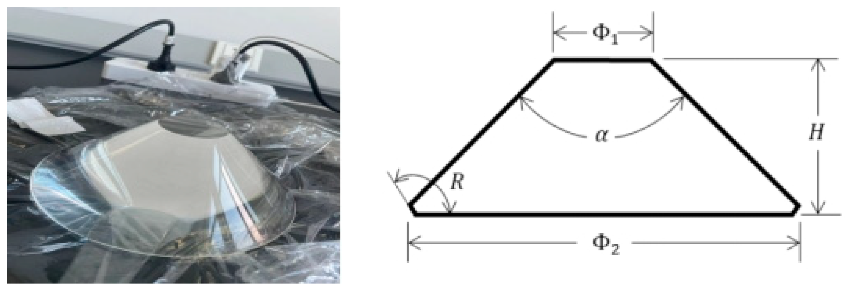
Figure 1. Physical sample and sample structure.
Jmse 14 00151 g001
Figure 2. (a). Positions of external strain gauges and measured directions. (b). Positions of internal strain gauges and measured directions.
Jmse 14 00151 g002aJmse 14 00151 g002b
Figure 3. Pressurization load variation.
Jmse 14 00151 g003
Figure 4. Overall strain variation.
Jmse 14 00151 g004
Figure 5. Maximum principal stress variation over time.
Jmse 14 00151 g005
Figure 6. Strain variation on the external surface.
Jmse 14 00151 g006
Figure 7. Correlation coefficients.
Jmse 14 00151 g007
Figure 8. CNN architecture.
Jmse 14 00151 g008
Figure 9. LSTM architecture.
Jmse 14 00151 g009
Figure 10. CNN-LSTM model.
Jmse 14 00151 g010
Figure 11. Structure of the transformer–CNN–BiLSTM model.
Jmse 14 00151 g011
Figure 12. (a). Fitting line of the GP model. (b). Fitting line of the CNN-LSTM model. (c). Fitting line of the transformer–CNN-BiLSTM model.
Jmse 14 00151 g012aJmse 14 00151 g012b
Figure 13. (a). Fitting line of the GP model. (b). Fitting line of the CNN-LSTM model. (c). Fitting line of the transformer–CNN–BiLSTM model.
Jmse 14 00151 g013aJmse 14 00151 g013b
Figure 14. (a). Prediction results of the GP model. (b). Prediction results of the CNN-LSTM model. (c). Prediction results of the transformer–CNN–BiLSTM model.
Jmse 14 00151 g014
Figure 15. (a). Prediction results of the GP model. (b). Prediction results of the CNN-LSTM model. (c). Prediction results of the transformer–CNN–BiLSTM model.
Jmse 14 00151 g015
Figure 16. Comparison of first dataset metrics.
Jmse 14 00151 g016
Figure 17. (a) Variations in the CNN-LSTM metrics using the first dataset. (b) Variations in the transformer–CNN–BiLSTM metrics using the first dataset.
Jmse 14 00151 g017
Figure 18. Comparison of the second dataset metrics.
Jmse 14 00151 g018
Figure 19. (a). Variations in the CNN-LSTM metrics using the second dataset. (b). Variations in the transformer–CNN–BiLSTM metrics using the second dataset.
Jmse 14 00151 g019
Table 1. Mechanical parameters of the PMMA samples.
Technical SpecificationsNumerical Values
Density (g/cm3)1.186
Tensile modulus/GPa3.13
Yield strength/MPa129
Poisson’s ratio0.37
Refractive index1.49
Elasticity modulus/MPa3540
Table 2. MSE, MAE, and RSR values of the three models.
MSEMAERSR
Transformer-CNN-BiLSTM0.01830.09540.1353
CNN-LSTM0.05910.12740.2432
GP1.177011.220831.0849
Table 3. MSE, MAE, and RSR values of the three models.
MSEMAERSR
Transformer-CNN-BiLSTM0.23980.30010.4897
CNN-LSTM0.348060.36160.5899
GP5.6746.59686.892
Disclaimer/Publisher’s Note: The statements, opinions and data contained in all publications are solely those of the individual author(s) and contributor(s) and not of MDPI and/or the editor(s). MDPI and/or the editor(s) disclaim responsibility for any injury to people or property resulting from any ideas, methods, instructions or products referred to in the content.