Abstract
In this study, we developed a novel water quality model that integrated hydrodynamic, solute transport, and geochemical reactions processes. This model was built upon the open-source ELCIRC hydrodynamic model, the TVD-format solute transport model, and the PhreeqcRM geochemical reaction engine. The accuracy of the model was rigorously validated using a 2D chain decay analytical solution, demonstrating its capability to accurately simulate water flow, solute transport, and chemical reactions. To evaluate the practical applicability of the model, case studies involving the 2012 Huaihe River benzene leakage accident and the acetic acid leakage accident in the Gulei sea area were simulated. Findings indicate that the model effectively captures the diffusion and attenuation dynamics of the benzene contamination plume. Furthermore, it accurately depicts the reaction–diffusion interaction with seawater following acetic acid release. Notably, the versatility and flexibility of the model were further demonstrated by its ability to simulate a wide range of pollutants and their associated biochemical processes. This addresses the limitations of existing water quality models and provides a powerful tool for environmental monitoring and assessment. The results of this study offer valuable insights for improving water quality management and emergency response strategies in the face of environmental pollution incidents.
1. Introduction
Water serves as the fundamental source of life. Rivers and lakes, serving as important water resources, are vital for human survival and living. However, the contamination of these aquatic ecosystems has become progressively severe, primarily due to the extensive discharge of both industrial and municipal wastewater, alongside the accidental leakage of hazardous chemicals. This situation adversely impacts the quality of life for inhabitants and impedes societal development and progress. In recent years, several persistent and sudden environmental pollution accidents have caused significant damage to the local surface water environment, which has caused great losses to both human lives and property. Consequently, the protection of surface water resources has emerged as an urgent and critical issue that requires immediate resolution.
The surface water quality model, based on partial differential equations describing the transport, mixing, and migration of pollutants in surface water, is an effective tool for surface water pollution analysis. Early hydrodynamic numerical simulation research mainly focused on 1D and 2D numerical models. In 1871, Saint-Venant proposed the Saint-Venant equation [1], which opened up a new direction of numerical simulation of fluids and provided a theoretical basis for transient flow. The advancement of computer technology has ushered in a new era of rapid development for hydrodynamics numerical simulation, leading to the emergence of excellent methods such as the finite element method, finite difference method, and operator splitting method. In recent years, many numerical hydrodynamic models have emerged, including the HAMSOM model [2], the POM model [3], the ELCIRC model [4], and the Delft3D model [5]. Qin [6] used the narrow slit method to simulate tidal waves during the change in the boundary water level and achieved relatively good results; Wang [7] successfully used a wind-generated circulation model for a lake with a 3D hydrodynamic simulation; and Peng [8] promoted a finite volume method in the numerical calculation of 2D tidal currents.
The numerical modeling of solute or heat transport processes in natural waters is crucial for evaluating pollution issues within aquatic environments. In surface water environments, the Lagrangian particle tracking method and the convective diffusion model based on the Euler equations are frequently used [9]. Researchers [7,10,11,12] have demonstrated that the Lagrangian particle tracking method can simulate the trajectory of the solute. However, the accuracy of the result is significantly influenced by the number of particles released, making this method computationally intensive. In some cases, this method also fails to provide a clear visualization of the solute’s diffusion process [13]. The convective diffusion modeling method, when solving the convective diffusion equations, highly depends on the accuracy of the flow field obtained from numerical hydrodynamic simulations. Therefore, high-precision numerical methods are required to reduce the artificial diffusion and numerical oscillations in the discrete process [14]. Consequently, numerous higher-order formats have been investigated, including the Godunov format, approximate Riemann format [15], Total Variation Diminishing (TVD) format [16], and Essentially Non-Oscillatory (ENO) format [17]. At present, the TVD format is extensively employed in the numerical modeling of both structured and unstructured grids [18,19,20,21,22,23].
The water quality model is used to simulate the physical, chemical, ecological, and other interactions and patterns of change among solutes in rivers, lakes, and other water bodies [24]. For the last few years, some researchers have progressively integrated kinetic response modules into the advection–diffusion equations to formulate tightly coupling models. PHREEQC [25] is a sophisticated geochemical modeling software that has been developed from the chemical simulation program PHREEQE to simulate all types of chemical reactions with a variety of solutes, whereas PhreeqcRM [26] is built on PHREEQC [25] for performing equilibrium and kinetic reaction calculations. Widely used water quality models such as WASP, EFDC, and MIKE typically embed fixed sets of biogeochemical reaction modules, which are limited to conventional pollutants (e.g., nitrogen, phosphorus, dissolved oxygen). These models lack the flexibility to incorporate complex or non-standard geochemical processes, such as organic acid-driven mineral dissolution, redox transformations involving emerging contaminants, or custom aqueous speciation, without extensive code modification. This rigidity significantly restricts their applicability in scenarios involving accidental chemical spills, acid mine drainage, or carbon sequestration leakage, where dynamic and diverse chemical reactions play a critical role. In contrast, the integration of hydrodynamic models with PhreeqcRM [26], utilizing its powerful and extensible geochemical capabilities to complete the chemical part of the water quality model, has become a novel and promising approach for reaction modeling. PhreeqcRM enables the simulation of any reaction defined in the PHREEQC [25] thermodynamic database, including multi-phase equilibria, surface complexation, and kinetic reactions, without altering the core hydrodynamic code. This plug-and-play architecture provides unprecedented adaptability for simulating a wide range of real-world pollution scenarios [27].
The application of water quality models has been constrained by the excessive variety of pollution types and the complexity of pollutant properties and reactions. Most of the water quality models can only simulate the mixing, transport, and transformation of specified pollutants, not for non-target pollutants. No water quality model with wide coverage and versatility is reported. In contrast to previous studies, which often rely on idealized scenarios or limited datasets, this study presents a novel and practical approach by validating the integrated model using actual environmental accident data, which is rarely performed in the current literature. This provides a more realistic and reliable assessment of the model’s performance under real-world conditions. Furthermore, our 2D coupled hydrodynamic-solute transport-chemical reaction model, built upon the open-source ELCIRC hydrodynamic model and the geochemical reaction engine PhreeqcRM, overcomes the limitations of traditional models by incorporating comprehensive chemical reactions and achieving high computational efficiency through OpenMP acceleration.
2. Method
2.1. Hydrodynamic and Solute Transport Reaction Equations
The governing equations of ELCIRC are derived from the standard Navier–Stokes equations under the hydrostatic assumption and the Boussinesq approximation.
Momentum equation:
where t is the time [s]; u [m s−1] and v [m s−1] are the velocity components in the x and y directions (Cartesian coordinate system), respectively; is the free surface water level [m]; and is other forcing terms in the momentum equation (baroclinic pressure gradient force (), horizontal viscosity, earth tide potential, coriolis force, atmospheric pressure, radiation stress).
Vertically integrated continuity equation:
where is the vertical velocity [ms−1].
Depth-integrated continuity equation:
Transport equation:
where is the tracer concentration (salinity, temperature, sediment, etc.); is the vertical eddy viscosity and diffusivity for tracers [ms−1]; and is the horizontal diffusion and source-sink terms for substances.
For the 2D solute transport problem, it is assumed that variations in solute concentration are negligible in the vertical direction. Consequently, the depth-integrated equation for convection–diffusion of 2D solute transport can be derived as follows (Equation (1)):
where C is the depth-averaged solute concentration [g L−3]; Kxx, Kxy, Kyx, and Kyy are the components of the 2D diffusion coefficient tensor [m2 s−1]. R represents the reaction term. The coefficients can be calculated according to Preston [28] (Equations (2)–(4)),
where θ is the angle of the flow direction regarding the x-axis [−], and KL [m2 s−1] and KT [m2 s−1] are the diffusion coefficients along the longitudinal and transverse directions, respectively. These two diffusion coefficients can be estimated as follows (Equations (5) and (6)) [29]:
where c is Chèzy’s coefficient [m1/2 s−1]; α and β are two constant coefficients [−], with theoretical values close to 5.93 and 0.15 in a fully developed boundary layer of a straight channel [30] and close to 13 and 1.2, respectively, as the flow turbulence intensifies [31]. Under these and other conditions, the ratios of α to β and KL to KT are typically much greater than 1, resulting in anisotropic diffusion.
The operator splitting method is employed to segregate the equation into convective, diffusive, and reaction terms as follows (Equations (7)–(9)), and a different numerical method is applied to each term to improve the accuracy of the convective and diffusive terms [14,32,33]:
Advection:
Diffusion:
Reaction:
Equations (7) and (8) are differentially computed using the finite volume method and the alternating operator splitting step [32]. The operators are computed as follows (Equations (10)–(12)):
where Ladv is the convection operator and Ldiff is the diffusion operator, and R represents the reaction process.
Kong et al. [23] proposed an improved numerical scheme for solving the convective term using the finite volume method and anisotropic term from the Green formula, which satisfies the conservation of matter and the maximum–minimum principle. For details, refer to Kong et al. [23].
In reactivity modeling, kinetic reactions are very important. In PhreeqcRM, kinetic reactions are usually characterized by rate expressions. The RATES data in PhreeqcRM could be used to define a variety of reaction rate expressions, including multi-order Mono equations, equations taking into account inhibitory factors, and kinetic equations of any order [34]. Rate equations involving kinetic reactions of aqueous solutes can generally be written as follows (Equation (13)) [35]:
where ci is the concentration of the solutes i; v is the stoichiometric coefficient; N is the number of kinetic reactions; and Rjk is the degradation reaction rate of reaction jk.
In terms of solute transport, PhreeqcRM uses either an explicit Runge-Kutta or implicit CVODE equation solver, which allows for the simultaneous integration of multiple rate equations [36].
2.2. Water Quality Model Coupling
2.2.1. Coupled Water Quality Modeling Techniques
The chemical reaction model PhreeqcRM (Table 1) is coupled with a hydrodynamic-solute transport model. A flow chart of the two main processes of the initialization and the execution of the reaction is shown in Figure 1.

Table 1.
Create PhreeqcRM.
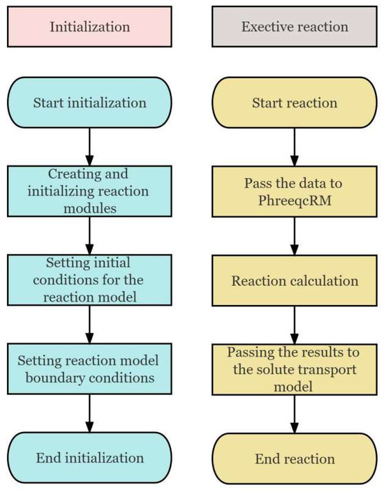
Figure 1.
Flow chart of reactive transport simulator.
In the numerical method of PhreeqcRM, the hydrogen (H) and oxygen (O) concentrations in the solution should be accurately distinguished to correctly calculate the pH and Pe values of the solution. It is also helpful to the stability of the calculations that H and O are distinguished in water and non-water. By using the RM_SetComponentH2O(id, tf) function, this determines whether water in the substance transport list can be set. The RM_Create mapping (id, grid2chem) function can be utilized to establish mapping between the hydrodynamic-solute transport grid and the chemical reaction grid. The integer array grid2chem (nxyz) can then be assigned appropriately to minimize the number of superfluous reaction grids, thereby conserving computational time.
Generally, the representative volume (RV) of each reaction unit is 1 L, and the water content (lc) of each reaction unit is calculated as follows (Equation (14)):
where S is saturation, n is porosity, and RV is representative volume. Saturation, porosity, and representative volume are set through the functions RM_SetSaturation(id, sat), RM_SetPorosity(id, por), and RM_SetRepresentativeVolume(id, rv), respectively. To make the reaction model solution concentration units consistent with the transport model, we set the concentration units with the function RM_SetUnitsSolution(id, option), and this procedure is automatically implemented by PhreeqcRM.
Initial conditions include the solution composition of the reaction unit, the amount of solutes, and the type of chemical reaction. Each reaction unit can be initialized by reading the Phreeqc input file and using the specified functions in PhreeqcRM. The boundary conditions of the model are set through the RM_InitialPhreeqc2Concentrations(id, bc_conc, nbound, bc1), which essentially assigns the solution concentrations in the input processing instance InitialPhreeqc to the real array of boundary concentrations, bc_conc (nbound, ncomps) (Table 2 and Table 3).
Table 2.
Set the initial conditions of the reaction model.
Table 3.
Set the boundary conditions of the reaction model.
Before reaction calculations, various parameters of each reaction unit need to be passed to PhreeqcRM at each time step. These parameters include the pressure, saturation, porosity, temperature, density, and concentration of the reaction units using the functions RM_SetPressure(id, p), RM_SetSaturation(id, sat), RM_SetPorosity(id, por), RM_SetTemperature(id, t), RM _SetConcentrations(id, c), and RM_SetDensity(id, density), respectively, for setting conditions (Table 4).
Table 4.
Data transfer and reaction calculations.
2.2.2. Parallel Computing Techniques in Water Quality Modeling
To deal with the large amount of computation, the coupled model is parallelized based on the OpenMP technique. In general, the following three principles need to be observed to successfully parallelize the target program [37]: I. Correctness principle. The computational results of the serial program and the parallel program must be the same. II. High-performance principle. The parallel computation time is smaller than the serial computation time. III. Scalability principle. Avoid drastically modifying the parallel program due to the availability of new hardware in case of rapid hardware changes. For this water quality model, parallel technology mainly includes hydrodynamic model parallel technology, solute transport model parallel technology, and chemical reaction model parallel technology.
Regarding hydrodynamic model parallel technology, firstly, the OpenMP header file can be announced at the beginning of the source program with a statement. The OMP_SET_NUM_THREADS () function in the OpenMP library function is to set the number of threads that will work together to perform the task in subsequent parallel regions, and parallel directives (! $OMP PARALLEL (clause list) and ! $OMP END PARALLEL) are to specify the beginning and end of a parallel; finally, ! $OMP DO and ! $OMP END DO instructions are to parallelize the loop structure.
Regarding the solute transport model parallel technique, the first three steps are consistent with the hydrodynamic model, and the fourth step is parallelized differently due to the different hotspots of the solute transport model program. We use the SECTIONS instruction to realize the segmented parallelism of the transport of different solutes.
On parallel techniques for chemical reaction modeling, PhreeqcRM supports MPI and OpenMP parallel computing, and different parallel acceleration methods are selected according to different use cases.
3. Model Calibration
Figure 2 shows the validation phase of the model. Initially, the soil column was filled with NaNO3-KNO3 solution, and the system achieved exchange equilibrium with the cationic adsorbent X present in the soil matrix. Upon commencement of the simulation, the soil column was flushed with CaCl2 solution. It was assumed throughout the simulation that Ca2+, K+, and Na+ remained in continuous equilibrium with the cation adsorbent X.
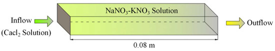
Figure 2.
Schematic diagram of a 1D model considering ion exchange.
The total length of the soil column was 0.08 m and discretized into 40 grid cells with the size of each grid being 0.002 m. The velocity of the CaCl2 solution was 2.778 × 10⁻⁶ m s−1 (Table 5), the simulation period was 72,000 s, the model time step was 720 s, and the cation exchange capacity of the adsorbent in the soil column was 0.0011 Eq L−1. The initial solution of NaNO3-KNO3 and flushing solution CaCl2 were composed as shown in Table 5.
Table 5.
Composition of initial solution and eluent.
The equilibrium reaction between the cation adsorbent and each dissolved cation determines the order of the ion penetration profile observed in the effluent [38]. Within this model, Ca2+ exchange exhibits the most robust activity, followed by K+, with Na+ exchange demonstrating the least strength.
Figure 3 shows the Cl− breakthrough curve of the effluent without the ion diffusion considered. Because the ion exchange reactions did not take place, its concentration changes abruptly from 0 to 1.2 mmol kg w−1 when the flushing solution CaCl2 moves to the end of the soil column. The breakthrough curve of Na+ initially remained unchanged, subsequently exhibiting a decrease. This alteration was primarily attributed to the model’s weakest exchange capacity for Na+. In the same way, the breakthrough curve of K+ initially remained unchanged, subsequently increased, and ultimately decreased. This pattern was attributed to the superior exchange capacity of K+ compared to Na+ in the model under consideration. The concentration surged when a substantial amount of adsorbed K+ was exchanged from the soil columns. Conversely, as the adsorbed K+ was progressively depleted, a decline in concentration ensued. As the adsorbed K+ in the soil column is progressively depleted, a corresponding decrease in concentration is observed. The breakthrough curve for Ca2+ was zero at the beginning and then gradually increased to a stable concentration in the flushing solution; this is due to its strongest exchange capacity, which becomes detectable in the effluent when the original adsorbed Na+ and K+ in the soil column are gradually depleted.
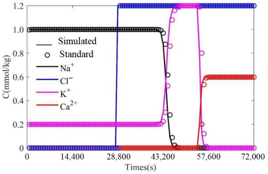
Figure 3.
Comparison of breakthrough curves by coupling model and PHREEQC.
During the initial phase of the simulation, the cationic adsorbent in the soil column reached equilibrium with the initial solution NaNO3-KNO3 reaction in case the adsorbate was composed of NaX or KX. With the inflow of the CaCl2 solution, the cations in the original NaX and KX were exchanged, leading to the adsorbate composition being NaX, KX, and CaX2. When all the original NaX and KX in the soil column had been exchanged, only CaX2 remained in the adsorbate at this point.
The simulated values of the model agreed well with the simulated values, indicating the correctness of the coupling model developed in this study.
4. Applications
4.1. Case Study of Hazardous Chemical Spills in Inland Waters
4.1.1. Study Area
At 22:10 on 28 February 2012, an explosion occurred 3.6 km downstream of the Bengbu lock of the Huaihe River, resulting in benzene-containing wastewater spillage into the Huaihe River’s mainstream. According to the Environmental Quality Standards for Surface Water (GB 3838-2002 [39]), the concentration of benzene in surface water should not be more than 0.01 mg L−1. In order to safeguard the water quality of the downstream source, both the local government and the Huaihe River Water Resources Commission promptly implemented measures for water disposal. The discharge of the Bengbu lock was reduced, and activated carbon was put into the polluted water body to adsorb contaminants at three different river sections.
After the pollution accident occurred, the Huaihe River Basin Water Resources Protection Bureau monitored benzene concentrations at 20 cross sections downstream to accurately figure out the plume of benzene. Figure 4 shows the riverside area affected by this accident and the location of the monitoring cross-sections; to facilitate the analysis, the study area is divided into 10 sections (Figure 4).
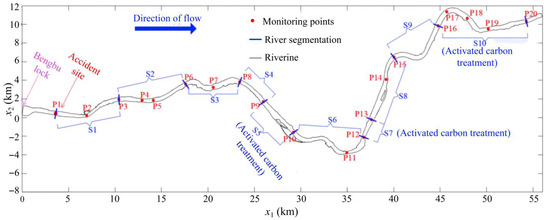
Figure 4.
Overview of the study area.
The hydrodynamic model of the Huaihe River Basin is a 2D model, and the model grid is an unstructured triangular grid with 41,035 elements and 22,632 nodes. The topographic interpolation of the grid was performed by taking the measured topographic data of the study area, with the inlet on the left side of the river and the outlet on the right side. The inlet boundary is set as a sequence of flux through the Bengbu lock bar from 28 December 2012 to 13 January 2013, and the outlet boundary condition is set as a sequence of water levels at the outlet section over the corresponding time.
At the inlet position, P1 is the benzene leakage point shown in Figure 4. The timely measured value of P1 is set as the inlet concentration boundary. The outlet concentration boundary was set to the zero-concentration gradient. Typical values of diffusion coefficient D in the Huaihe River Basin (Table 6) range from 1.5 to 9.7 [40], and the diffusion coefficient was 5 in this simulation [41].
Table 6.
The attenuation coefficient of each river section.
The decay process of benzene in the water quality modeling includes volatilization, activated carbon adsorption, and natural attenuation. PhreeqcRM is utilized as the kinetic reaction module. The decay rate of benzene was from the RATES data block. The details of model validations can be found in the Appendix A and Appendix B.
4.1.2. Simulations and Studies Under Different Cases
To further investigate the effectiveness of the disposal measures, four cases are considered in this section: Case A represents the actual situation, with the flow control and activated carbon adsorption; Case B with the activated carbon adsorption and without flow control; Case C with the flow control and without activated carbon adsorption; and Case D without flow control and activated carbon adsorption.
Figure 5 presents the curve of maximum concentration (Cm) at the cross-section under different cases. The maximum concentration at the cross-section decreased from monitoring point P1 to P20 due to the river’s dilution effect and benzene’s attenuation effect. In the activated carbon input river section (depicted in gray within the Figure), both Cases A and B exhibited a notable reduction in the maximum concentration across the cross-section. This observation underscores the efficacy of activated carbon in significantly diminishing the peak concentration of benzene-contaminated plumes.
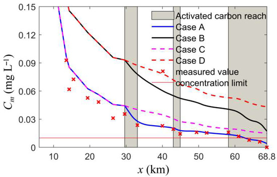
Figure 5.
Maximum concentration curve of the section under different cases.
The variation curves of benzene concentration at each monitoring point under the four different cases are shown in Figure 6. Both Cases A and B show that the lack of flow control results in not only an earlier peak arrival time of the benzene-contaminated plume but also a significant increase in the peak concentration. This is mainly due to the flow increase, which leads to an increased velocity and average channel depth, reducing the dilution, decay time, and volatilization coefficient of the benzene-contaminated plume, consequently leading to a significant increase in the peak concentration. The same conclusion can be drawn for Case C compared to D.
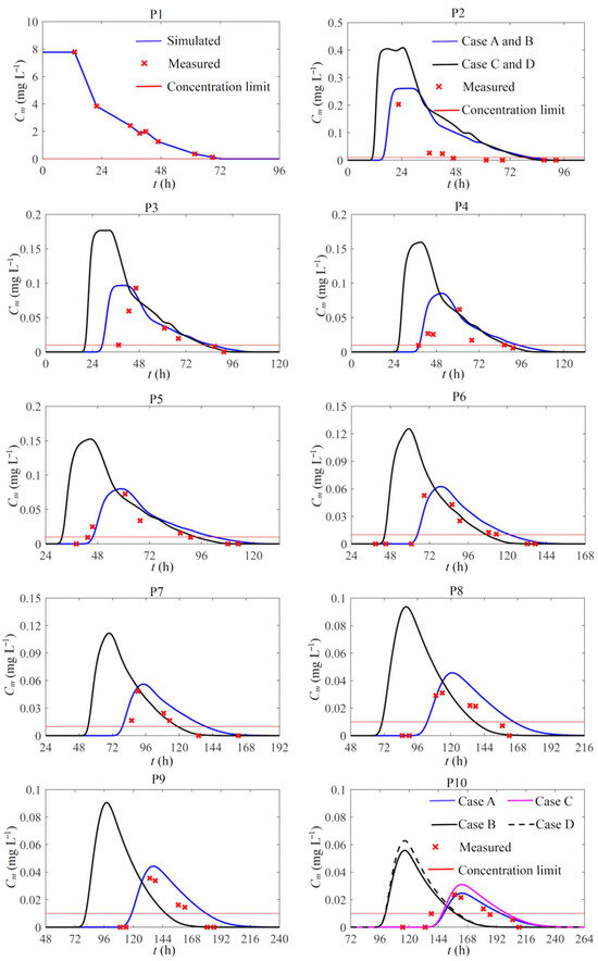
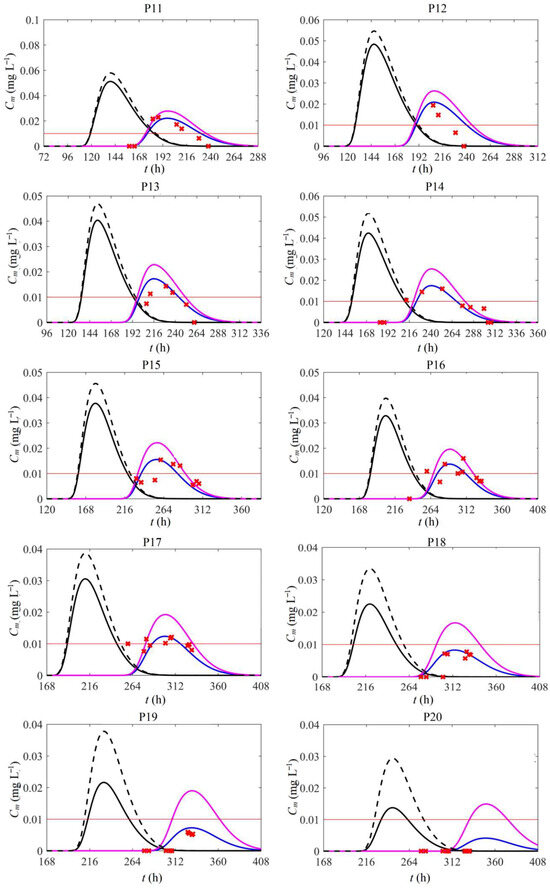
Figure 6.
Measured and simulated concentration process of benzene at each monitoring point under different cases.
As observed in Cases A and C, the activated carbon significantly reduced the peak concentration of the benzene-contaminated plume but did not change the peak arrival time. The same conclusion can be obtained for Case B compared to D. In a word, Case A is the most effective and Case D is the least effective. It indicates that both flow control and activated carbon adsorption are effective in reducing the peak concentration of the benzene-contaminated plume.
Three phases of benzene removed from river water were the volatilization phase, activated carbon adsorption phase, and natural attenuation phase. Simulation results are shown in Table 7; the removed benzene was mainly in the volatile and activated carbon adsorption phases. In Case A, only about 12% of the benzene was in the natural decay phase, around 39% was in the volatile phase, and 48% was activated carbon adsorption phase. In Cases C and D, most of the removed benzene was in the volatile phase, suggesting that volatilization is the dominant form of benzene attenuation in the absence of activated carbon adsorption. Case C and Case D show that the volatile phase percentage decreases as the flow increases.
Table 7.
Distributions of benzene in different cases.
To further assess the movement characteristics of the benzene pollution plume in the river section under the four scenarios, the spatial and temporal range curves of the benzene pollution plume under the different scenarios are shown in Figure 7. The range of the curves under the scenarios also showed the tendency to decrease, followed by increase, then relative stability, and finally another decrease. This was mainly related to the relative magnitude of convective diffusion and attenuation at the various stages.
Figure 7.
Spatial and temporal extent of the benzene pollution zone in different cases.
For Case A, the total duration of benzene pollution in the river (Tm) was about 300 h, affecting a river section of about 60 km downstream of the Bengbu lock. It indicates that the two measures can effectively reduce benzene pollution. The remaining three cases are not effective in controlling benzene pollution, and there is a risk of contamination downstream. From Cases A and C, the range of the curves is significantly reduced in the sections by activated carbon, which further illustrates the ability of activated carbon to significantly reduce the range of benzene contamination and decrease the duration of contamination (TL). From Cases A and B, an increase in velocity decreases the total benzene contamination duration (Tm) but expands the extent of benzene contamination.
4.2. Acid-Base Balance Analysis of Nearshore Waters
4.2.1. Study Area
Gulei Harbor is located on the west side of Dongshan Bay. Figure 8 shows the contour of water depth and the hydrologic observation points (T1 and C1). The coral reef nature reserve is located on the southwest side of Gulei Harbor, as shown in Figure 9.
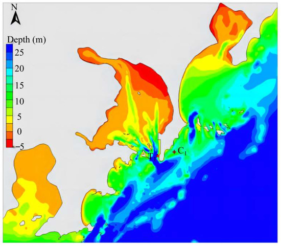
Figure 8.
Location diagram of observation points in December 2013.
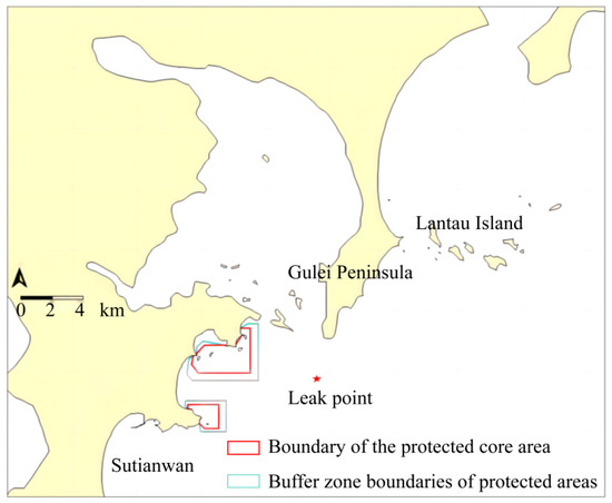
Figure 9.
The location of the incident.
The tidal current in the Gulei Sea area is an irregular semi-diurnal shallow sea current. The tidal current movement form is mainly reciprocating flow. The leakage of acetic acid happens when low and flat tides are present. The leakage continued for about 1.5 h, and the model period is 72 h. The leakage location was chosen at the intersection of the Gulei channel and Dongshan branch channel (Figure 9), and the total amount of leakage was taken as 1000 t. Model validation is in the Appendix A and Appendix B.
4.2.2. Analysis of Model Results
Acetic acid will react with various ions in the ocean when spilled, and the main reactions involving acetate are shown in Table 8. In addition, acetic acid also reacts with the carbon dioxide–carbonate system in seawater to form CH3COO− as follows (Equations (15)–(17)):
Table 8.
Main reaction equations involving acetate.
Simulation results show that the four solutes, CH3COO−, CH3COOH, CH3COOMg+, and CH3COONa, account for more than 98% at any moment, indicating that the majority of the leaked acetic acid exists in these four forms after reacting with seawater.
Figure 10 illustrates the mass of CH3COO−, CH3COOH, CH3COOMg+, and CH3COONa after an acetic acid spill. During the duration of the leak (0–1.5 h), the CH3COO−, CH3COOMg+, and CH3COONa masses increased sharply due to the large amount of acetic acid leakage in a short period. The mass of CH3COOH shows a trend of increasing and then decreasing because the mass consumed by the reaction between CH3COOH and seawater is smaller than the mass leaked into the seawater at the early stage of the leakage. However, at the late stage of the leakage, with the diffusion of CH3COOH by hydrodynamics, the area of reaction with seawater increased, so the mass consumed by the reaction between CH3COOH and seawater is larger than the mass leaked into seawater, showing a decreasing trend.
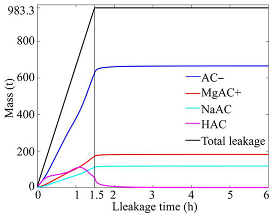
Figure 10.
Mass change curve of solutes containing acetate.
Following the leakage, CH3COO−, CH3COOMg+, and CH3COONa increased slightly and then tended to be constant, while the mass of CH3COOH decreased rapidly and finally lowered to zero. Since there was still a small amount of CH3COOH in the seawater after the leakage, CH3COOH was consumed by seawater; the mass of CH3COOH eventually decreased to zero, while the mass of CH3COO−, CH3COOMg+, and CH3COONa first increased and then remained constant.
Table 9 demonstrates the various components and total mass of acetate in the 72 h sea area; the magnitude of the percentage of the final form of leaking acetic acid present was CH3COO− > CH3COOMg+ > CH3COONa > CH3COOCa+ > CH3COOK > (CH3COO)2Mg > (CH3COO)2Ca > (CH3COO)2Na− > (CH3COO)2K− in accordance with the reaction rate constants and the concentrations of the reactants.
Table 9.
Type and mass of acetate in the sea area (t = 72 h).
Figure 11 shows the comparison between the simulated values and the standard value of the concentration of each component of the inorganic carbon at the leakage point. The simulated values of the concentration of each component can meet the standard value very well, indicating that the CO2–carbonate system simulated by the coupled model can correctly respond to the actual situation.
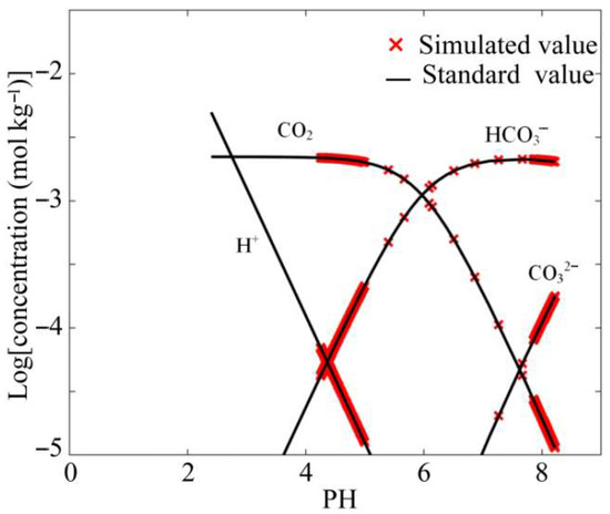
Figure 11.
Simulated value of each component concentration of inorganic carbon at leakage point.
Figure 12a demonstrates the trends of the concentrations of HCO3−, CO32−, H+, and CO2 at the leakage point over time from 0 to 3 h. During the leakage stage, due to the large amount of leaking acetic acid, the CO2–carbonate system drastically changes, the concentrations of HCO3− and CO32− decrease, and the concentration of CO2 increases, while the pH decreases. When the leak is over, the CO2–carbonate system quickly recovers due to hydrodynamic diffusion effects.
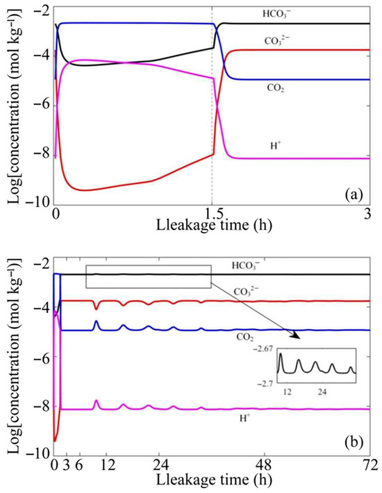
Figure 12.
Variation in the concentration of every component of inorganic carbon at the leakage point. (a) 0−3 h, (b) 0−72 h.
Figure 12b illustrates the trend of the concentration of HCO3−, CO32−, H+, and CO2 in the leak point cell with time throughout the simulation time. The concentration of each component shows periodic fluctuation with time, including the concentration of HCO3− and H+. The concentration of CO2 periodically increases, and the concentration of CO32− periodically decreases. The range of fluctuation is gradually decreasing, and the concentration of each component stays relatively stable after experiencing five more obvious cycles. The main reason for the periodicity of the concentration of each component is that the sea area has irregular semi-diurnal shallow currents, and the form of current movement is mainly reciprocating, which results in the periodic change in the concentration of each component. The gradual decrease in the range of fluctuation of each component is mainly due to the strong buffering effect of seawater.
It should be noted that the trend of HCO3− concentration in the leakage time changed in the subsequent diffusion time, which is mainly due to the different acid–base environments. In the acidic environment of the leakage phase, an increase in solution pH leads to a decrease in HCO3− concentration [42]. In contrast, in the later diffusion phase, the H+ concentration is always in an alkaline environment, although it periodically increases, and an increase in solution pH leads to an increase in HCO3− concentration.
Subsequently, the entire sea area was studied to analyze the changes in the concentrations of CO2, H+, and CaCO3 after the acetic acid spill. The amount of CO2 gas in seawater is usually expressed in terms of the partial pressure of CO2 (pCO2) in μatm, which in combination with Henry’s law and can be used to calculate the concentration of CO2 gas dissolved in seawater (Equation (18)):
where K0 is Henry’s constant for CO2 in seawater as follows (Equation (19)):
where T = t + 273.15.
It is proven that raising partial pressures of CO2 in seawater could lead to seawater acidification, coral reef bleaching [43], and an increase in the proportion of aberrant and incomplete phytoplankton pellets [44]. Esbaugh [45] studied the effects of CO2 partial pressure magnitude on marine scleractinian fish in 2012 and showed that acidosis occurred in fish after 15 min of exposure to 1000 and 1900 μatm CO2 partial pressure. We used the results of Esbaugh’s study and plotted the area of CO2 partial pressure exceedance versus time using 1000 μatm as the exceedance level, as shown in Figure 13.
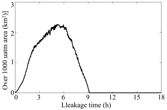
Figure 13.
Temporal development of the excess area of CO2 partial pressure.
The results show that the area of CO2 partial pressure exceedance generally followed a trend of increasing and then decreasing. At the initial stage of the leakage, the exceedance area increased due to the convective diffusion effect of the tidal current. Subsequently, due to the strong buffering effect of seawater, the exceedance area decreased rapidly, and the CO2 partial pressure exceedance area disappeared in approximately 9 h. The 24 h envelope and hour-by-hour concentration contour of CO2 partial pressure in the sea area are shown in Figure 14.
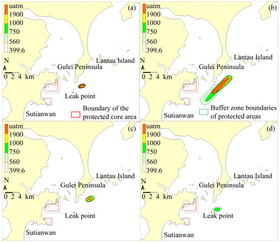
Figure 14.
Distribution of CO2 partial pressure in sea area. (a) 24 h envelope, (b) 3 h, (c) 6 h, and (d) 9 h concentration distributions.
Acidification of seawater due to acetic acid leakage also causes the dissolution of CaCO3 in seawater. It has been shown that the dissolution of calcium carbonate in seawater restricts the shell growth of calcareous shelled organisms in the ocean [44,46,47], which can severely affect the stability of the euphotic zone ecosystem. Figure 15 illustrates the envelope of calcium carbonate concentration distribution after an acetic acid spill.
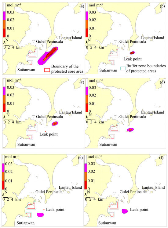
Figure 15.
Distribution of CaCO3 in sea area. (a) 24 h envelope, (b) 3 h, (c) 6 h, (d) 9 h, (e) 12 h, and (f) 15 h concentration distributions.
5. Conclusions
This study coupled the hydrodynamic model ELCIRC, the solute transport model in TVD format, and the geochemical package PhreeqcRM to establish a 2D surface water quality model of hydrodynamic-solute transport-chemical reactions. The key findings are as follows:
The model was validated by a 2D chain decay analytical solution. Results showed that the model in this paper can accurately simulate the water flow, solute transport, and chemical reaction processes.
The model was applied to the simulation of benzene leakage in the Huaihe River in 2012 and calibrated by measured data. The dispersion of benzene pollution in the river under different scenarios was also simulated. Results showed that increased flow would increase the dispersion range and peak concentration of the benzene pollution plume, reduce the duration of benzene pollution in the watershed, and decrease the percentage of the volatile phase of benzene in the river. In contrast, the input of activated carbon significantly reduces the spreading range, peak concentration, and duration of benzene pollution plume in the watershed.
The model was applied to the simulation of the acetic acid water quality process in the Gulei Harbor area of Xiamen Port. The spilled acetic acid reacts rapidly with seawater and becomes mostly CH3COO−, a small portion as CH3COOMg+ and CH3COONa, and a very small portion in other forms; in addition, it can cause changes in the carbon dioxide–carbonate system in seawater.
In terms of applicability, the proposed model excels in simulating complex aqueous-phase geochemical reactions, such as acid–base equilibria, redox transformations, mineral dissolution/precipitation, and metal–organic complexation, within shallow, well-mixed surface water bodies. Its integration with PhreeqcRM provides exceptional flexibility for modeling non-standard or emerging contaminants (e.g., organic acids, heavy metals, industrial chemicals) without requiring code-level modifications. However, the current 2D vertically averaged formulation limits its use in strongly stratified or deep-water systems where vertical gradients are critical. Moreover, the model does not yet incorporate biodegradation, photolysis, or air–water gas exchange processes. Therefore, it is best suited for short-to-medium-term simulations of reactive pollutant spills in rivers, estuaries, and nearshore coastal zones, particularly scenarios involving rapid inorganic or organic aqueous chemistry, such as chemical accidents or acid discharges.
Author Contributions
Conceptualization, J.K. and Q.T.; methodology, S.H.; software, Q.T.; validation, K.W. and S.H.; formal analysis, S.H.; investigation, K.W.; resources, J.K.; data curation, K.W.; writing—original draft preparation, Q.T.; writing—review and editing, K.W., Q.T. and S.H.; visualization, S.H.; funding acquisition, J.K. All authors have read and agreed to the published version of the manuscript.
Funding
This research was supported by the National Key R&D Program of China (2021YFB2600200) and the National Natural Science Foundation of China (42576225).
Data Availability Statement
Some or all data, models, or code that support the findings of this study are available from the corresponding author upon reasonable request.
Conflicts of Interest
The authors declare no conflicts of interest.
Appendix A. Model Validation
Appendix A.1. Case Study of Hazardous Chemical Spills in Inland Waters
As shown in Figure A1, the coupled model predictions of the 20 monitoring points were in good agreement with the measured values as well as the concentration trends. Results of the mean absolute error (MAE) and root mean square error (RMSE) (Table A1) are reasonable and vary within a small range. These results show that the measured values and the predicted values of the model simulation fit well, and the established coupled model can be applied to the simulation of benzene pollution leakage in the Huaihe River.
Table A1.
Benzene concentration error value at each monitoring point.
Appendix A.2. Acid–Base Balance Analysis of Nearshore Waters
The model is designed to be a nested mathematical model, using the large model to provide boundary conditions for the small model, i.e., the China Sea tidal wave model, a local mathematical model in the engineering area. The tidal wave model of the China Sea was used in the large model, with boundaries provided by the reconciliation constants; the boundaries of the small model are given in Figure A1. The measured and simulated concentration process of benzene at each monitoring point is noted, water level boundaries are obtained from the actual simulation of the large model, and the modeling domain includes the whole of Dongshan Island, Gulei Peninsula, and Nan’ao Island.
To better represent the complex characteristics of the bay in the Gulei Sea, the model computational mesh was set as the non-structural triangular mesh, and the mesh is refined in the vicinity of the leakage point; the total number of non-structural grids is 83,834, and the total number of cell nodes is 43,059.
The validation data is based on the measured data of Foutou Bay located on the north side of Dongshan Island, and the specific station layout is given (Figure 8). The values of the resistive Manning’s coefficient in the model validation range from 0.010 to 0.016, and the periods of the model are from 00:00 of 17 December 2013 to 00:00 of 27 December 2013, respectively. High tide: 18 December 2013 to 19 December 2013; medium tide: 22 December 2013 to 23 December 2013; low tide: 25 December 2013 to 26 December 2013.
Based on the tide level data in December 2013, the validation results show that the model-calculated values are in good agreement with the measured tide level (such as T1); see Figure A2. According to Figure A3, the validation of the mean flow velocity process of the spring tide at observation point (C1) shows that the model-calculated values are in good agreement with the measured tidal levels, and the flow velocity process is generally consistent with the field.
To verify that PhreeqcRM can correctly simulate the various reactions of acetic acid, we reproduce the acetic acid titration curves versus the concentration of each inorganic carbon component in seawater as a function of pH using PhreeqcRM. As strong acids, the shape of the titration curve for weak acids depends strongly on the properties of the acid and the corresponding ionization constant (Ka). The titration curves of HAC, HCl solution, and NaOH solution were plotted using PhreeqcRM (Figure A4), PhreeqcRM was able to reproduce the characteristics of the titration curves very well and was also able to match the values of the titration standards very well. The solid black line represents the titration curve for the titration of 0.1 mol L−1 HAC solution with 0.2 mol L−1 NaOH solution, while the dashed line represents the titration curve for the titration of 0.1 mol L−1 HCl solution with 0.2 mol L−1 NaOH solution.
To verify that PhreeqcRM can correctly simulate the reaction between acetic acid and seawater, as well as to understand the reaction that occurs with seawater after the leakage of acetic acid, and to provide a basis for subsequent coupled modeling, we investigated the changes in the seawater carbon dioxide–carbonate system following the addition of acetic acid to seawater. To reproduce the change curves of the concentration of each inorganic carbon component in seawater with pH value, PhreeqcRM was used to simulate the change in the concentration of each inorganic carbon component after adding glacial acetic acid to seawater (Figure A5). It can be seen that PhreeqcRM can reproduce the variation rules of CO2, HCO3−, and CO32− well, and it also matches well with the concentration standard values.


Figure A1.
Measured and simulated concentration process of benzene at each monitoring point.


Figure A2.
Verification of tide level process at Gulei Station (T1).


Figure A3.
Verification of flow velocity and direction during spring tide. (a) velocity validation; (b) flow direction validation.


Figure A4.
Comparison of titration simulation value and standard value.


Figure A5.
Simulated value of the concentration of inorganic carbon components in seawater changing with pH value.

The acetic acid coupling model largely aligns with Section 3, exhibiting only minor discrepancies. Firstly, different chemical coupling models use different Phreeqc files. Secondly, the reaction simulation of acetic acid using PhreeqcRM requires the use of the llnl.dat database file, so it is necessary to load llnl.dat in the program (Table A2). Finally, the reaction of acetic acid with seawater requires the use of the PhreeqcRM ion transport module, which is different from the solute transport module and uses different functions (Table A2). A total of 45 solutes were selected for transport using the PhreeqcRM ion transport module, as shown in Table A3.
Table A2.
Multicomponent-diffusion transport module.
Table A3.
Name and initial concentration of transported solutes.
Appendix B. Results
The results are shown in Table A4.
Table A4.
Type and mass of acetate in the sea area (t = 72 h).
References
- Barré de Saint-Venant, A.-J.-C. Théorie du Mouvement Non Permanent des Eaux, Avec Application aux Crues des Rivières et à L’introduction des Marées Dans Leur Lit; Gauthier-Villars: Paris, France, 1871. [Google Scholar]
- Backhaus, J.O. A Three-Dimensional Model for the Simulation of Shelf Sea Dynamics. Dtsch. Hydrogr. Z. 1985, 38, 165–187. [Google Scholar] [CrossRef]
- Blumberg, A.; Mellor, G. A Description of a Three-Dimensional Coastal Ocean Circulation Model. In Three-Dimensional Coastal Ocean Models; American Geophysical Union: Washington, DC, USA, 1987; Volume 4. [Google Scholar] [CrossRef]
- Zhang, Y.; Baptista, A.M.; Myers, E.P. A Cross-Scale Model for 3D Baroclinic Circulation in Estuary–Plume–Shelf Systems: I. Formulation and Skill Assessment. Cont. Shelf Res. 2004, 24, 2187–2214. [Google Scholar] [CrossRef]
- Delft Hydraulics, W.L. Delft3D-FLOW: Simulation of Multi-Dimensional Hydrodynamic Flows and Transport Phenomena, Including Sediments—User Manual. In Report of Delft Hydraulics; Deltares: Delft, The Netherlands, 2003. [Google Scholar]
- Qin, Z.H.; Hu, S.; Cheng, L.Q. Tidal simulation in the adjacent sea area of Cook Strait based on FVCOM. Coast. Eng. 2025, 44, 173–185. [Google Scholar] [CrossRef]
- Wang, J.; Shen, Y.; Guo, Y. Seasonal Circulation and Influence Factors of the Bohai Sea: A Numerical Study Based on Lagrangian Particle Tracking Method. Ocean Dyn. 2010, 60, 1581–1596. [Google Scholar] [CrossRef]
- Peng, D.; Mao, J.; Li, J.; Zhao, L.; Peng, D.; Mao, J.; Li, J.; Zhao, L. Tidal Current Modeling Using Shallow Water Equa-tions Based on the Finite Element Method: Case Studies in the Qiongzhou Strait and Around Naozhou Island. Sustainability 2025, 17, 1256. [Google Scholar] [CrossRef]
- Peng, H.; Yao, Y.-M.; Liu, L. Study on the Features of Water Exchange in Xiangshangang Bay. J. Mar. Sci. 2012, 30, 1–12. [Google Scholar]
- Provenzale, A.; Babiano, A.; Villone, B. Single-Particle Trajectories in Two-Dimensional Turbulence. Chaos Solitons Fractals 1995, 5, 2055–2071. [Google Scholar] [CrossRef]
- Korotenko, K.A.; Mamedov, R.M.; Kontar, A.E.; Korotenko, L.A. Particle Tracking Method in the Approach for Prediction of Oil Slick Transport in the Sea: Modelling Oil Pollution Resulting from River Input. J. Mar. Syst. 2004, 48, 159–170. [Google Scholar] [CrossRef]
- Liu, W.-C.; Chen, W.-B.; Hsu, M.-H. Using a Three-Dimensional Particle-Tracking Model to Estimate the Residence Time and Age of Water in a Tidal Estuary. Comput. Geosci. 2011, 37, 1148–1161. [Google Scholar] [CrossRef]
- Deleersnijder, E.; Delhez, E.J.M. Timescale- and Tracer-Based Methods for Understanding the Results of Complex Marine Models. Estuar. Coast. Shelf Sci. 2007, 74, 585–776. [Google Scholar] [CrossRef]
- Rubio, A.D.; Zalts, A.; El Hasi, C.D. Numerical Solution of the Advection–Reaction–Diffusion Equation at Different Scales. Environ. Model. Softw. 2008, 23, 90–95. [Google Scholar] [CrossRef]
- Roe, P.L. Approximate Riemann Solvers, Parameter Vectors, and Difference Schemes. J. Comput. Phys. 1997, 135, 250–258. [Google Scholar] [CrossRef]
- Harten, A. High Resolution Schemes for Hyperbolic Conservation Laws. J. Comput. Phys. 1997, 135, 260–278. [Google Scholar] [CrossRef]
- Harten, A.; Engquist, B.; Osher, S.; Chakravarthy, S.R. Uniformly High Order Accurate Essentially Non-Oscillatory Schemes, III. J. Comput. Phys. 1987, 71, 231–303. [Google Scholar] [CrossRef]
- Frink, N.T. Upwind Scheme for Solving the Euler Equations on Unstructured Tetrahedral Meshes. AIAA J. 1992, 30, 70–77. [Google Scholar] [CrossRef]
- Tamamidis, P. A New Upwind Scheme on Triangular Meshes Using the Finite Volume Method. Comput. Methods Appl. Mech. Eng. 1995, 124, 15–31. [Google Scholar] [CrossRef]
- Gross, E.S.; Koseff, J.R.; Monismith, S.G. Evaluation of Advective Schemes for Estuarine Salinity Simulations. J. Hydraul. Eng. 1999, 125, 32–46. [Google Scholar] [CrossRef]
- Mingham, C.G.; Causon, D.M.; Ingram, D.M. A TVD MacCormack Scheme for Transcritical Flow. Proc. Inst. Civ. Eng. Water Marit. Eng. 2001, 148, 167–175. [Google Scholar] [CrossRef]
- Li, L.; Liao, H.; Qi, L. An Improved r-Factor Algorithm for TVD Schemes. Int. J. Heat Mass Transf. 2008, 51, 610–617. [Google Scholar] [CrossRef]
- Kong, J.; Xin, P.; Shen, C.-J.; Song, Z.-Y.; Li, L. A High-Resolution Method for the Depth-Integrated Solute Transport Equation Based on an Unstructured Mesh. Environ. Model. Softw. 2013, 40, 109–127. [Google Scholar] [CrossRef]
- Dong, W. A Review of Progress in Research on Water Quality Models in America. Water Resour. Hydropower Eng. 2006, 37, 68–73. [Google Scholar]
- Parkhurst, D.L.; Thorstenson, D.C.; Plummer, N. PHREEQE: A Computer Program for Geochemical Calculations; U.S. Geological Survey, Water Resources Division: Reston, VA, USA, 1980.
- Parkhurst, D.L.; Wissmeier, L. PhreeqcRM: A Reaction Module for Transport Simulators Based on the Geochemical Model PHREEQC. Adv. Water Resour. 2015, 83, 176–189. [Google Scholar] [CrossRef]
- FEFLOW® 6.2 User Manual 2012, DHI: Horsholm, Denmark, 2012.
- Preston, R.W. The Representation of Dispersion in Two-Dimensional Shallow Water Flow; Central Electricity Research Laboratories: Surrey, UK, 1985; Volume 84, pp. 1–13. [Google Scholar]
- Elder, J.W. The Dispersion of Marked Fluid in Turbulent Shear Flow. J. Fluid Mech. 1959, 5, 544–560. [Google Scholar] [CrossRef]
- Fischer, H.B. Longitudinal Dispersion and Turbulent Mixing in Open-Channel Flow. Annu. Rev. Fluid Mech. 1973, 5, 59–78. [Google Scholar] [CrossRef]
- Falconer, R.A. Review of Modelling Flow and Pollutant Transport Processes in Hydraulic Basins. In Water Pollution: Modelling, Measuring and Prediction; Wrobel, L.C., Brebbia, C.A., Eds.; Springer: Dordrecht, The Netherlands, 1991; pp. 3–23. ISBN 978-94-011-3694-5. [Google Scholar]
- Liang, D.; Wang, X.; Falconer, R.A.; Bockelmann-Evans, B.N. Solving the Depth-Integrated Solute Transport Equation with a TVD-MacCormack Scheme. Environ. Model. Softw. 2010, 25, 1619–1629. [Google Scholar] [CrossRef]
- Valocchi, A.J.; Malmstead, M. Accuracy of Operator Splitting for Advection-Dispersion-Reaction Problems. Water Resour. Res. 1992, 28, 1471–1476. [Google Scholar] [CrossRef]
- Steefel, C.I.; Appelo, C.A.J.; Arora, B.; Jacques, D.; Kalbacher, T.; Kolditz, O.; Lagneau, V.; Lichtner, P.C.; Mayer, K.U.; Meeussen, J.C.L.; et al. Reactive Transport Codes for Subsurface Environmental Simulation. Comput Geosci. 2015, 19, 445–478. [Google Scholar] [CrossRef]
- Jacques, D.; Šimůnek, J.; Mallants, D.; van Genuchten, M.T. Modeling Coupled Hydrologic and Chemical Processes: Long-Term Uranium Transport Following Phosphorus Fertilization. Vadose Zone J. 2008, 7, 698–711. [Google Scholar] [CrossRef]
- Cohen, S.D.; Hindmarsh, A.C.; Dubois, P.F. CVODE, A Stiff/Nonstiff ODE Solver in C. Comput. Phys. 1996, 10, 138–143. [Google Scholar] [CrossRef]
- Jin, H.; Jespersen, D.; Mehrotra, P.; Biswas, R.; Huang, L.; Chapman, B. High Performance Computing Using MPI and OpenMP on Multi-Core Parallel Systems. Parallel Comput. 2011, 37, 562–575. [Google Scholar] [CrossRef]
- Rolle, M.; Sprocati, R.; Masi, M.; Jin, B.; Muniruzzaman, M. Nernst-Planck-based Description of Transport, Coulombic Interactions, and Geochemical Reactions in Porous Media: Modeling Approach and Benchmark Experiments. Water Resour. Res. 2018, 54, 3176–3195. [Google Scholar] [CrossRef]
- GB3838-2002; Environment Quality Standards for Surface Water. Ministry of Ecology and Environment of the People’s Republic of China: Beijing, China, 2002.
- Deng, Z.-Q.; Bengtsson, L.; Singh, V.P.; Adrian, D.D. Longitudinal Dispersion Coefficient in Single-Channel Streams. J. Hydraul. Eng. 2002, 128, 901–916. [Google Scholar] [CrossRef]
- Jin, G.; Zhang, Z.; Yang, Y.; Hu, S.; Tang, H.; Barry, D.A.; Li, L. Mitigation of Impact of a Major Benzene Spill into a River through Flow Control and In-Situ Activated Carbon Absorption. Water Res. 2020, 172, 115489. [Google Scholar] [CrossRef]
- Emerson, S.R.; Hamme, R.C. Chemical Oceanography: Element Fluxes in the Sea, 1st ed.; Cambridge University Press: Cambridge, UK, 2022; ISBN 978-1-316-84117-4. [Google Scholar]
- Bellwood, D.; Hughes, T.; Folke, C.; Nyström, M. Confronting the Coral Reef Crisis. Nature 2004, 429, 827–833. [Google Scholar] [CrossRef] [PubMed]
- Riebesell, U.; Zondervan, I.; Rost, B.; Tortell, P.D.; Zeebe, R.E.; Morel, F.M.M. Reduced Calcification of Marine Plankton in Response to Increased Atmospheric CO2. Nature 2000, 407, 364–367. [Google Scholar] [CrossRef]
- Esbaugh, A.J.; Heuer, R.; Grosell, M. Impacts of Ocean Acidification on Respiratory Gas Exchange and Acid–Base Balance in a Marine Teleost, Opsanus Beta. J. Comp. Physiol. B 2012, 182, 921–934. [Google Scholar] [CrossRef]
- Zondervan, I.; Zeebe, R.E.; Rost, B.; Riebesell, U. Decreasing Marine Biogenic Calcification: A Negative Feedback on Rising Atmospheric pCO2. Glob. Biogeochem. Cycles 2001, 15, 507–516. [Google Scholar] [CrossRef]
- Langdon, C.; Broecker, W.S.; Hammond, D.E.; Glenn, E.; Fitzsimmons, K.; Nelson, S.G.; Peng, T.; Hajdas, I.; Bonani, G. Effect of Elevated CO2 on the Community Metabolism of an Experimental Coral Reef. Glob. Biogeochem. Cycles 2003, 17, 1020. [Google Scholar] [CrossRef]


Disclaimer/Publisher’s Note: The statements, opinions and data contained in all publications are solely those of the individual author(s) and contributor(s) and not of MDPI and/or the editor(s). MDPI and/or the editor(s) disclaim responsibility for any injury to people or property resulting from any ideas, methods, instructions or products referred to in the content. |
© 2026 by the authors. Licensee MDPI, Basel, Switzerland. This article is an open access article distributed under the terms and conditions of the Creative Commons Attribution (CC BY) license.