Multi-Horizon Significant Wave Height Forecasting Along Guangdong–Hong Kong Coast Using Tropical Cyclone Trajectory Information

Abstract

Accurate forecasting of significant wave height (SWH) during tropical cyclones (TCs) is important for coastal risk management. This study develops a multi-horizon TC-aware sequence-to-sequence (MH-TCSeq2Seq) framework for 12 and 24 h lead time forecasting at eight Guangdong–Hong Kong stations, utilizing marine and historical TC data as baseline inputs. An enhanced variant integrated with 6–24 h future TC trajectory information (MH-TCSeq2Seq-FutureTC) is further established using retrospective best track data as an idealized upper bound benchmark. Evaluation against the ERA5 reanalysis data shows that MH-TCSeq2Seq-FutureTC achieves the lowest overall root mean square error (RMSE), reaching 0.207 m at 12 h and 0.307 m at 24 h. It reduces the TC-associated RMSE by 9.6% and 7.3% relative to the MH-TCSeq2Seq baseline. Statistical validation confirms the overall robustness of this forecasting improvement across TC events. Adding identical future TC predictors to Quantile Bidirectional Gated Recurrent Unit and TC-gated Bidirectional Gated Recurrent Unit degrades performance, indicating that such benefits are architecture dependent. Replacing these track inputs with operational forecast descriptors from the Automated Tropical Cyclone Forecasting System still reduces the TC-associated RMSE by 6.1% and 4.7% relative to MH-TCSeq2Seq. Interpretability analyses confirm the model’s reliance on future TC information for improving SWH forecasting.

1. Introduction

The South China Sea and its adjacent coastal zones are among the regions that are most frequently affected by tropical cyclones (TCs), where storm-induced extreme waves pose serious risks to maritime safety, coastal infrastructure, and offshore operations [1,2]. Significant wave height (SWH), defined as the average height of the highest one-third of waves in a given sea state, is a primary parameter for characterizing ocean wave intensity in both scientific research and operational forecasting [3,4]. Along the Guangdong and Hong Kong coasts, historical TCs such as Super Typhoon Hato (2017) and Mangkhut (2018) generated severe waves and storm surges, causing widespread coastal inundation and substantial economic losses in the Pearl River Delta region [2,5]. Accurate and timely SWH forecasting is therefore essential for disaster preparedness, navigational safety, port operations, and coastal protection.

The Guangdong–Hong Kong coastal waters are also recognized as a priority area for offshore wind energy development [6,7]. Wave conditions, particularly SWH, directly affect wind-farm construction and operation, including foundation installation, cable laying, vessel operability, and turbine fatigue loading. Consequently, accurate SWH forecasting in this region is not only essential for disaster mitigation but also a prerequisite for the safe and cost-effective utilization of offshore wind energy.

Third-generation numerical wave models, including SWAN (Simulating WAves Nearshore) [8], WAVEWATCH III [9], and WAM [10], have long been widely used for SWH forecasting. Despite their strong physical foundations, numerical forecasting systems may retain substantial biases under both normal and extreme weather conditions, largely due to coarse wind field representation and simplified wave interaction parameterizations [11,12]. This limitation motivates the development of complementary data-driven forecasting and correction approaches [13]. TC-induced wave prediction is particularly challenging because the sea state is jointly controlled by cyclone intensity, storm size, storm-site relative position, and the time-dependent evolution of the wind field [2,14,15,16]. These processes produce strongly nonlinear and rapidly evolving wave responses that are difficult to represent accurately, especially at longer forecast horizons.

Machine-learning methods for SWH forecasting have progressed from early artificial neural networks and support vector regression models [17,18] to recurrent architectures based on long short-term memory networks, which are capable of learning temporal dependencies in oceanographic time series [19,20,21]. More recently, transformer-based and foundation model-inspired sequence architectures have also shown potential in wave forecasting applications [22,23]. However, several issues remain insufficiently addressed for coastal SWH prediction during TC-affected periods.

First, many data-driven studies focus primarily on overall deterministic performance, without separately evaluating TC-associated and non-TC conditions. This makes it difficult to determine whether model improvements remain effective during storm-affected periods, when wind forcing, storm proximity, and swell propagation change rapidly [23,24,25]. Although recent studies have investigated TC-induced waves through approaches such as buoy observations, case analyses of extreme weather events in the South China Sea, and TC characteristic descriptors, systematic stratified evaluations across multiple coastal stations and forecast horizons remain limited [24,26,27].

Second, dedicated multi-station studies are still needed to quantify the spatial variability of TC period forecast performance along complex coastlines [24,26]. In addition, most existing TC-aware models use concurrent or historical storm descriptors, such as maximum sustained wind speed, central pressure, and storm-site distance [27]. The value of TC trajectory information over the forecast window, the dependence of that value on the model architecture, and the effect of replacing retrospective best track inputs with forecast track guidance available at initialization remain insufficiently explored.

To address these gaps, this study develops a multi-horizon TC-aware sequence-to-sequence (MH-TCSeq2Seq) framework for 12 and 24 h SWH forecasting at eight coastal and offshore stations along the Guangdong–Hong Kong coast. The framework adopts separate encoding pathways for marine variables and historical TC evolution. The proposed MH-TCSeq2Seq further combines TC-aware information fusion with multi-horizon decoding, allowing local marine conditions and TC evolution to be represented separately before their interaction is learned for multi-horizon forecasting. A future tropical cyclone (FutureTC) branch is introduced to provide forecast window TC trajectory descriptors over the 6–24 h period. The same future TC predictors are also incorporated into the Q-BiGRU and TG-BiGRU models to examine whether their predictive value depends on the model architecture. Two complementary experiments are conducted: future TC descriptors are retrospectively derived from best track records and treated as an idealized upper bound configuration; and another experiment replaces the best-track-derived future TC inputs with forecast guidance from the Automated Tropical Cyclone Forecasting System (ATCF) available at initialization, referred to as FutureATCF, to assess operational applicability.

Accordingly, this study aims to: (1) evaluate overall forecasting performance and compare model skill under TC-associated and non-TC conditions at the 12 and 24 h horizons; (2) quantify the spatial-, event scale-, and architecture-dependent contributions of the forecast window TC trajectory information; (3) assess the architecture dependence through reduced recurrent baselines; and (4) examine operational relevance through forecast track replacement and model reliance using SHapley Additive exPlanations (SHAP) and group permutation diagnostics. By explicitly incorporating forecast window TC evolution, this study seeks to clarify when, where, and under which model configurations future TC information can improve coastal SWH forecasting.

2. Materials and Methods

2.1. Study Area and Data

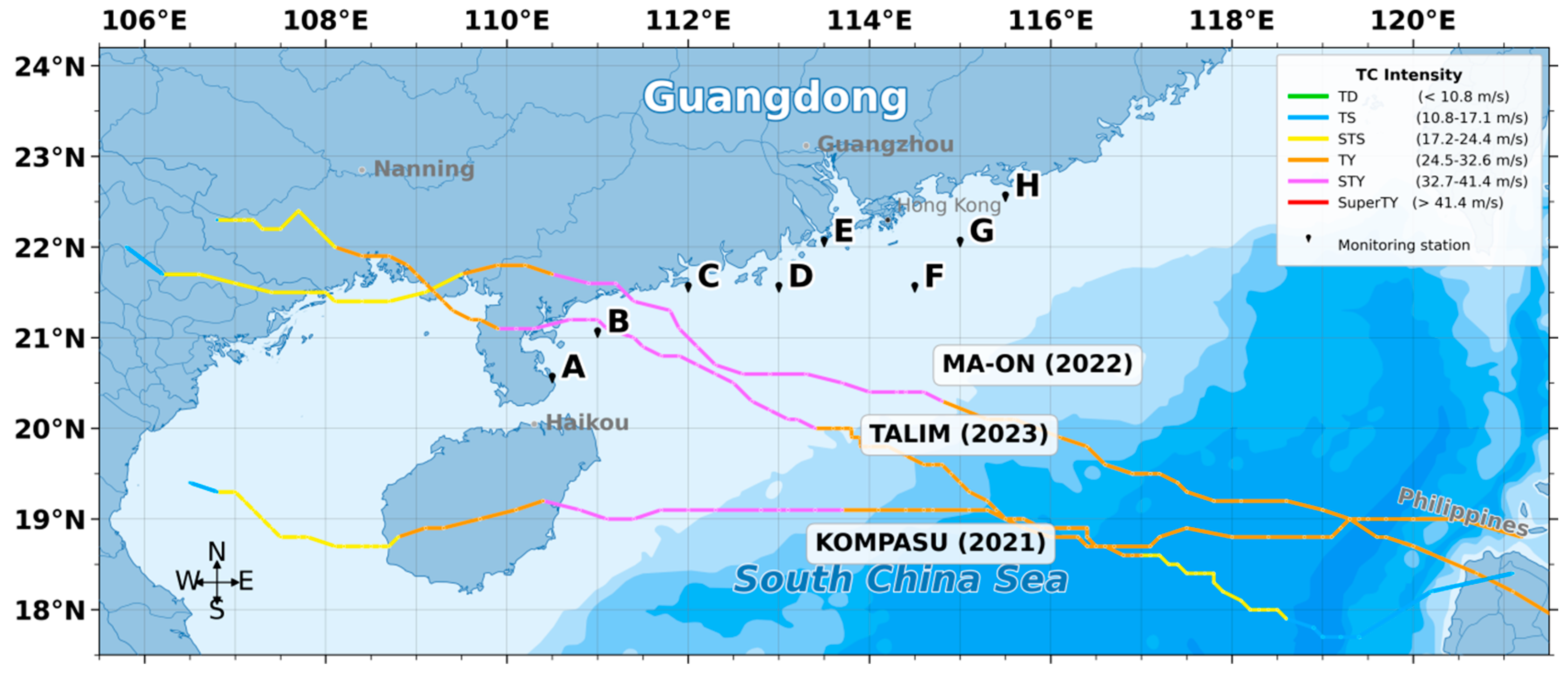
This study focuses on eight representative coastal and offshore stations (A–H) along the Guangdong–Hong Kong coasts of the South China Sea (Figure 1). The locations span approximately 5° of longitude (110.5° E to 115.5° E) and 2° of latitude (20.5° N to 22.5° N), covering about 600 km of coastline from the Leizhou Peninsula in the west to the eastern Guangdong coast. The stations can be grouped into three segments: western Guangdong (Stations A–C), the Pearl River Delta (Stations D–E), and the eastern open coast (Stations F–H)—all within priority zones for offshore wind energy development [6,7].

This study uses two datasets spanning from 2008 to 2023. TC best track data, including maximum sustained wind speed (Vmax), central pressure, geographic position, and TC size (radius of gale force winds, R34), are obtained from the China Meteorological Administration (CMA). Hourly atmospheric and wave variables, such as wind speed and direction, wave height, period, and direction, are extracted from the fifth-generation reanalysis dataset of the European Centre for Medium-Range Weather Forecasts (ERA5) [28]. Atmospheric variables have a spatial resolution of 0.25°, while wave variables adopt a 0.5° resolution. The target variable (Y) is SWH at the future times of 12 and 24 h. The potential predictor variables (X) include all relevant atmospheric, wave, and TC track features. In addition to current TC characteristics, we also incorporate future TC track variables representing the forecasted TC intensity, distance, and approach azimuth at the future lead times of 6, 12, 18, and 24 h (5 variables × 4 lead time horizons). All input and output variables are listed in

Table 1. Input and output variables used in the forecasting framework.

Category	Variable	Description	Unit
Input Local marine variables	WHmax	Maximum individual wave height	m
	P_WHmax	Period corresponding to maximum individual wave height	s
	MWP	Mean wave period	s
	NWS	10 m neutral wind speed	m/s
	NWS_6h	Rolling mean of 10 m neutral wind speed over the preceding 6 h	m/s
	NWS_12h	Rolling mean of 10 m neutral wind speed over the preceding 12 h	m/s
	NWS_24h	Rolling mean of 10 m neutral wind speed over the preceding 24 h	m/s
	Hour_sin/cos	Sine and cosine components of hour-of-day cyclic encoding	—
	Month_sin/cos	Sine and cosine components of month-of-year cyclic encoding	—
	SWH_chan1h	1 h temporal change in significant wave height (SWH)	m
	SWH_chan3h	3 h temporal change in SWH	m
	MWD_sin/cos	Sine and cosine components of mean wave direction	—
	NWD_sin/cos	Sine and cosine components of 10 m neutral wind direction	—
Input TC track variables	Vmax	Current maximum sustained wind speed of the TC	m/s
	P_central	Current central pressure of the TC	hPa
	R34	Current radius of 34-knot winds of the TC	km
	Distance	Current great circle distance from the TC center to target station	km
	App_rate	Current TC approaching rate to the station	km/h
	App_acc	Current temporal change rate of TC approaching speed	km/h2
	Az_sin/cos	Current sine and cosine components of TC azimuth relative to the station	—
Input future TC track variables	F_Vmax	Maximum sustained wind speed of the TC at future lead times of 6, 12, 18, and 24 h	m/s
	F_Distance	Great circle distance from the TC center to target station at future lead times of 6, 12, 18, and 24 h	km
	F_Az_sin/cos	Sine and cosine components of TC azimuth relative to the station at future lead times of 6, 12, 18, and 24 h	—
	F_TC_flag	Binary flag indicating TC occurrence at future lead times of 6, 12, 18, and 24 h	0/1
Input Gate	TC_gate	Binary indicator used to activate or suppress the TC-aware gating branch	0/1
Output Forecast targets	SWH (t + 12)	Forecasted SWH at 12 h lead time	m
	SWH (t + 24)	Forecasted SWH at 24 h lead time	m

Notes: Sine/cosine pairs are used as two independent input features. Raw SWH is not used directly as a local input feature; only the 1 and 3 h historical SWH change features are retained. FutureTC branch contains five predictors: F_Distance, F_Az_sin, F_Az_cos, F_Vmax, and F_TC_flag. TC_gate is used as an auxiliary input for the TC-aware gating module.

.

2.2. Predictor Construction and Data Preparation

2.2.1. Input Features

Based on the variables listed in Table 1, the predictors are organized into three groups: local marine conditions, current TC track predictors, and future TC track variables, with an auxiliary binary gate TC_gate for the TC-aware gating module. The local marine conditions include ERA5-derived wave and wind variables: maximum individual wave height (WHmax), period corresponding to WHmax (P_WHmax), mean wave period (MWP), and 10 m neutral wind speed (NWS). Raw SWH is excluded from direct inputs, mainly to avoid target leakage. Feeding present time raw SWH would encourage the model to learn a naive persistence forecast rather than making full use of wind- and TC-related physical forcing. It is also strongly collinear with WHmax. Instead, short-term wave evolution is represented by temporal variation terms of historical SWH: 1 h and 3 h SWH-change terms (SWH_chan1h, SWH_chan3h).

Directional variables, such as the mean wave direction (MWD) and neutral wind direction (NWD), are converted into sine/cosine pairs to avoid numerical discontinuities at 0°/360°. This group also captures short-term wind persistence: rolling 6, 12, and 24 h average NWS series. Diurnal and annual periodicity is encoded via sine/cosine pairs for hour-of-day and month-of-year.

The current TC track predictor group (historical TC encoder branch) includes current variables: Vmax, central pressure (P_central), R34 (radius of 34-knot winds) [29], great circle distance between the TC center and target station, TC azimuth (encoded with sine/cosine), and the temporal evolution of the TC–station distance (App_rate and App_acc). The FutureTC branch provides forecast horizon TC information at lead times of 6, 12, 18, and 24 h, including F_Vmax, F_Distance, paired F_Az_sin/F_Az_cos, and a binary occurrence indicator F_TC_flag. If no TC occurs within 800 km of the station across all four forecast lead times (6, 12, 18, 24 h), the global gating input ‘TC_gate’ is set to 0, and the TC-aware gating module suppresses the entire FutureTC branch. Otherwise, ‘TC_gate’ activates the branch. For individual lead times, ‘F_TC_flag = 1’ denotes such a TC occurrence, where physical TC forecast values are adopted for ‘F_Distance’, ‘F_Az_sin’, ‘F_Az_cos’, and ‘F_Vmax’. For lead times without TC (F_TC_flag = 0), these predictors are assigned NaN as missing value markers.

A threshold of 800 km is adopted to define TC occurrence relative to the target station. This choice follows the outer-bound radial scale widely used in operational TC statistical prediction schemes such as the Statistical Hurricane Intensity Prediction Scheme (SHIPS) [30], where environmental predictors are averaged within the 200–800 km annulus surrounding the TC center. Physically, TC-generated swell waves can propagate up to 800 km [31], while beyond 800 km, the direct TC-related signal becomes negligible.

The TC approaching azimuth relative to each station is computed using spherical trigonometry [32]. The TC–station great circle distance is calculated using the haversine formula:

$$\mathrm{D}\mathrm{i}\mathrm{s}\mathrm{t}\mathrm{a}\mathrm{n}\mathrm{c}\mathrm{e}=2\mathrm{R}\mathrm{a}\mathrm{r}\mathrm{c}\mathrm{s}\mathrm{i}\mathrm{n}\sqrt{{\mathrm{s}\mathrm{i}\mathrm{n}}^2\left({\displaystyle \frac{{\mathit{\varphi }}_{\mathit{s}}\mathit{-}{\mathit{\varphi }}_{\mathit{t}\mathit{c}}}{2}}\right)+\cos \left({\mathit{\varphi }}_{\mathit{t}\mathit{c}}\right)\cos \left({\mathsf{\varphi }}_{\mathrm{s}}\right)\sin {\displaystyle \frac{{\mathit{\lambda }}_{\mathit{s}}\mathit{-}{\mathit{\lambda }}_{\mathit{t}\mathit{c}}}{2}}}$$

(1)

where Distance is the great circle distance, R is the mean Earth radius, ${\mathit{\varphi }}_{\mathit{t}\mathit{c}}$ and ${\mathit{\lambda }}_{\mathit{t}\mathit{c}}$ denote the latitude and longitude of the TC center, and ${\mathit{\varphi }}_{\mathit{s}}$ and ${\mathit{\lambda }}_{\mathit{s}}$ denote the latitude and longitude of the target station.

The TC approaching rate is defined as the negative first-order temporal difference of the TC–station distance:

$$\mathrm{A}\mathrm{p}\mathrm{p}\_\mathrm{r}\mathrm{a}\mathrm{t}\mathrm{e}\left(t\right)=-\left[\mathrm{D}\mathrm{i}\mathrm{s}\mathrm{t}\mathrm{a}\mathrm{n}\mathrm{c}\mathrm{e}\left(t\right)-\mathrm{D}\mathrm{i}\mathrm{s}\mathrm{t}\mathrm{a}\mathrm{n}\mathrm{c}\mathrm{e}\left(t-1\right)\right]$$

(2)

A positive value indicates that the TC is moving toward the station. The approaching acceleration is then defined as:

$$\mathrm{A}\mathrm{p}\mathrm{p}\_\mathrm{a}\mathrm{c}\mathrm{c}\left(t\right)=\mathrm{A}\mathrm{p}\mathrm{p}\_\mathrm{r}\mathrm{a}\mathrm{t}\mathrm{e}\left(t\right)-\mathrm{A}\mathrm{p}\mathrm{p}\_\mathrm{r}\mathrm{a}\mathrm{t}\mathrm{e}\left(t-1\right)$$

(3)

These two variables describe whether a TC is approaching or receding from the station and whether the approaching speed is increasing or decreasing.

2.2.2. Data Partitioning, Preprocessing, and Sequence Construction

The dataset is chronologically split into training (2008–2018), validation (2019–2020), and testing (2021–2023) periods, all based on TC best track records. Following the construction of the 24 h historical input sequences and a 24 h maximum forecast horizon, the partitions contain 771,659, 139,968, and 209,883 station-specific samples, respectively (

Table 2. Distribution of station-specific forecast samples obtained with a 24 h historical input window and a 24 h maximum forecast horizon.

Partition	Period	Total Samples	TC Associated, n (%)	Non-TC, n (%)	Distinct TC Events
Training	2008–2018	771,659	61,228 (7.93%)	710,431 (92.07%)	114
Validation	2019–2020	139,968	8833 (6.31%)	131,135 (93.69%)	25
Test	2021–2023	209,883	14,877 (7.09%)	195,006 (92.91%)	23

Note: Samples are station-specific sequence instances; adjacent hourly initializations share overlapping input windows and are not statistically independent. Distinct TC events are counted within each partition.

). TC-associated samples accounted for 7.93%, 6.31%, and 7.09% of these partitions, and the test set includes 23 distinct TCs. In addition, a complementary hindcast experiment is conducted over the 2021–2023 test period using forecast tracks from the Automated Tropical Cyclone Forecast (ATCF) system [33] to assess performance under more operationally realistic input conditions.

All continuous input variables and output targets are processed via robust scaling based on the median and interquartile range (IQR) [34]:

$${\mathit{x}}^{\prime }={\displaystyle \frac{\mathit{x}-\mathrm{m}\mathrm{e}\mathrm{d}\mathrm{i}\mathrm{a}\mathrm{n}\left(x\right)}{\mathrm{I}\mathrm{Q}\mathrm{R}\left(x\right)}}$$

(4)

where x is the raw variable and x′ is the scaled value. Robust scaling is preferred over standard z-score normalization because the median and IQR are less sensitive to heavy-tailed extreme wave values induced by TCs [34]. To avoid information leakage across data partitions, all scaling parameters are estimated from the training set and then applied without modification to the validation and test sets [35].

The forecasting task is formulated as a multi-horizon sequence learning problem. For each sample, a 24 h historical input window is constructed to generate simultaneous SWH forecasts at 12 and 24 h lead times.

2.3. Proposed MH-TCSeq2Seq Architecture

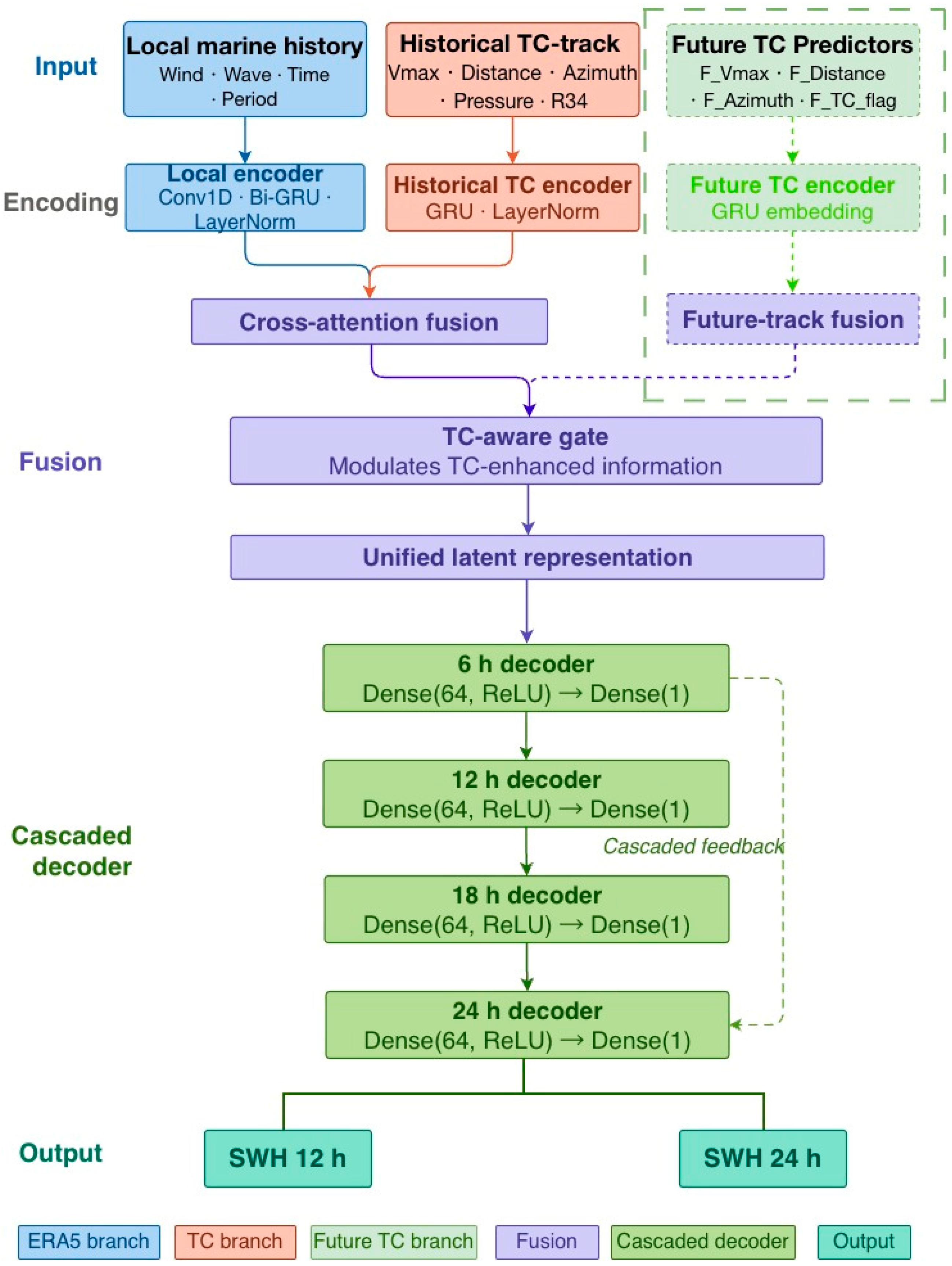
The proposed multi-horizon TC-aware sequence-to-sequence model, named MH-TCSeq2Seq, adopts two independent encoders to process local marine variables and historical TC track information separately. Its core workflow integrates cross-attention feature fusion, a TC-aware gating module, and cascaded multi-horizon decoders to jointly output SWH predictions at 12 and 24 h lead times. As an extended comparative model variant denoted MH-TCSeq2Seq-FutureTC, an extra dedicated FutureTC encoder branch is incorporated, which ingests future TC predictors including the forecasted TC distance, azimuth, intensity, and TC occurrence flag, as illustrated in Figure 2.

The core architecture contains two historical input branches. The local marine encoder extracts 24 h sequential features covering wave variables, wind, directional cyclic signals, and SWH temporal variations. The historical TC encoder processes the corresponding 24 h sequence of TC-related descriptors, including TC intensity, storm size, TC–station distance, azimuth, and dynamic approaching metrics (App_rate, App_acc). These two branches are designed to separately represent local sea state memory and historical TC evolution before feature fusion.

The encoded local marine and historical TC representations are fused using a multi-head cross-attention module [36], formulated as Equation (5), in which the marine features serve as query and the TC representations act as keys and values:

$$\mathrm{A}\mathrm{t}\mathrm{t}\mathrm{e}\mathrm{n}\mathrm{t}\mathrm{i}\mathrm{o}\mathrm{n}\left(\mathit{Q}\mathit{,}\mathit{K}\mathit{,}\mathit{V}\right)=\mathrm{S}\mathrm{o}\mathrm{f}\mathrm{t}\mathrm{m}\mathrm{a}\mathrm{x}\left({\displaystyle \frac{\mathit{Q}{\mathit{K}}^{\mathit{T}}}{\sqrt{{\mathit{d}}_{\mathit{k}}}}}\right)\mathit{V}$$

(5)

where ${\mathrm{d}}_{\mathrm{k}}$ denotes the dimensionality of the key vectors. This design allows the model to selectively extract TC-related information relevant to the evolving local sea state. The fused TC-enhanced representation is then modulated by TC_gate before being passed to the decoder. TC_gate is treated as a model input.

The MH-TCSeq2Seq-FutureTC variant adds a FutureTC encoder branch providing horizon-specific future TC information, such as F_Distance, F_Az_sin/F_Az_cos, F_Vmax, and F_TC_flag. These predictors represent the forecasted future TC–station geometry, TC intensity, and TC occurrence state, which are not included in the baseline MH-TCSeq2Seq model.

After cross-attention fusion and gate modulation, a cascaded multi-horizon decoder generates four SWH forecasts. The 6 h forecast representation is produced first and then passed forward to support the subsequent 12, 18, and 24 h forecasts. This decoder structure enables joint multi-horizon learning while allowing longer-lead-time predictions to benefit from shorter-lead-time forecast representations.

2.4. Model Comparison Design

The model comparison is implemented stepwise from a simple non-learning benchmark and recurrent baselines to the proposed framework and its FutureTC extended variant. This design enables separate evaluations of the contributions from learning-based sequential modeling, TC-aware conditioning mechanisms, multi-horizon Seq2Seq structural design, and future TC predictive inputs. Recurrent models are selected as learning-based baselines, as gated and bidirectional recurrent structures are widely used for sequence modeling and significant wave height forecasting [37,38,39,40].

The persistence forecast provides the simplest reference by propagating the latest SWH value to the forecast times. Quantile Bidirectional Gated Recurrent Unit (Q-BiGRU) serves as a basic recurrent baseline that learns temporal patterns from historical marine and TC variables. TC gated Bidirectional Gated Recurrent Unit (TG-BiGRU) adopts the same recurrent structure with an additional TC_gate input module. A comparison between Q-BiGRU and TG-BiGRU therefore evaluates the effectiveness of TC-aware conditioning in the recurrent baseline.

The proposed MH-TCSeq2Seq framework is described in Section 2.3. To assess the added value and architecture dependence of future TC information, the same future TC predictors are incorporated into MH-TCSeq2Seq, Q-BiGRU, and TG-BiGRU, forming the three FutureTC variants. Persistence and the two MH variants are evaluated at 6, 12, 18, and 24 h lead times, whereas the Q-BiGRU and TG-BiGRU baselines are evaluated at the common 12 and 24 h horizons. To assess the sensitivity to random initialization, MH-TCSeq2Seq and MH-TCSeq2Seq-FutureTC are additionally trained using five random seeds (42–46) under the same training settings. The station-balanced RMSE values at 12 and 24 h are summarized as the mean ± sample standard deviation across the five runs. Detailed model configurations and training hyperparameters are provided in Table S1. All models are implemented in Python (version 3.12) using TensorFlow (version 2.21.0), NumPy (version 2.5.0), and scikit-learn (version 1.8.0).

2.5. Performance Evaluation

The forecast accuracy over the 2021–2023 test period is evaluated using the root mean square error (RMSE), mean absolute error (MAE), and coefficient of determination $\left(R^2\right)$:

$$\mathrm{R}\mathrm{M}\mathrm{S}\mathrm{E}=\sqrt{{\displaystyle \frac{\mathrm{1}}{\mathit{N}}}{\sum }_{\mathit{i}\mathit{=}\mathrm{1}}^{\mathit{N}}{\left({\mathit{y}}_{\mathit{i}}\mathit{-}{\widehat{\mathit{y}}}_{\mathit{i}}\right)}^{\mathrm{2}}}$$

(6)

$$\mathrm{M}\mathrm{A}\mathrm{E}={\displaystyle \frac{1}{\mathit{N}}}{\sum }_{\mathit{i}=1}^{\mathit{N}}\left|{\mathit{y}}_{\mathit{i}}\mathit{-}{\widehat{\mathit{y}}}_{\mathit{i}}\right|$$

(7)

$${\mathit{R}}^2=1-{\displaystyle \frac{{\sum }_{\mathit{i}=1}^{\mathit{N}}{\left({\mathit{y}}_{\mathit{i}}\mathit{-}{\widehat{\mathit{y}}}_{\mathit{i}}\right)}^2}{{\sum }_{\mathit{i}=1}^{\mathit{N}}{\left({\mathit{y}}_{\mathit{i}}\mathit{-}\overline{\mathit{y}}\right)}^2}}$$

(8)

where ${\mathit{y}}_{\mathit{i}}$ is the ERA5 reference SWH, ${\widehat{\mathit{y}}}_{\mathit{i}}$ is the predicted SWH, and $\overline{\mathit{y}}$ is the mean reference value. These metrics are calculated separately for each forecast horizon. In addition to all sample evaluation, the metrics are also computed for TC-associated and non-TC samples.

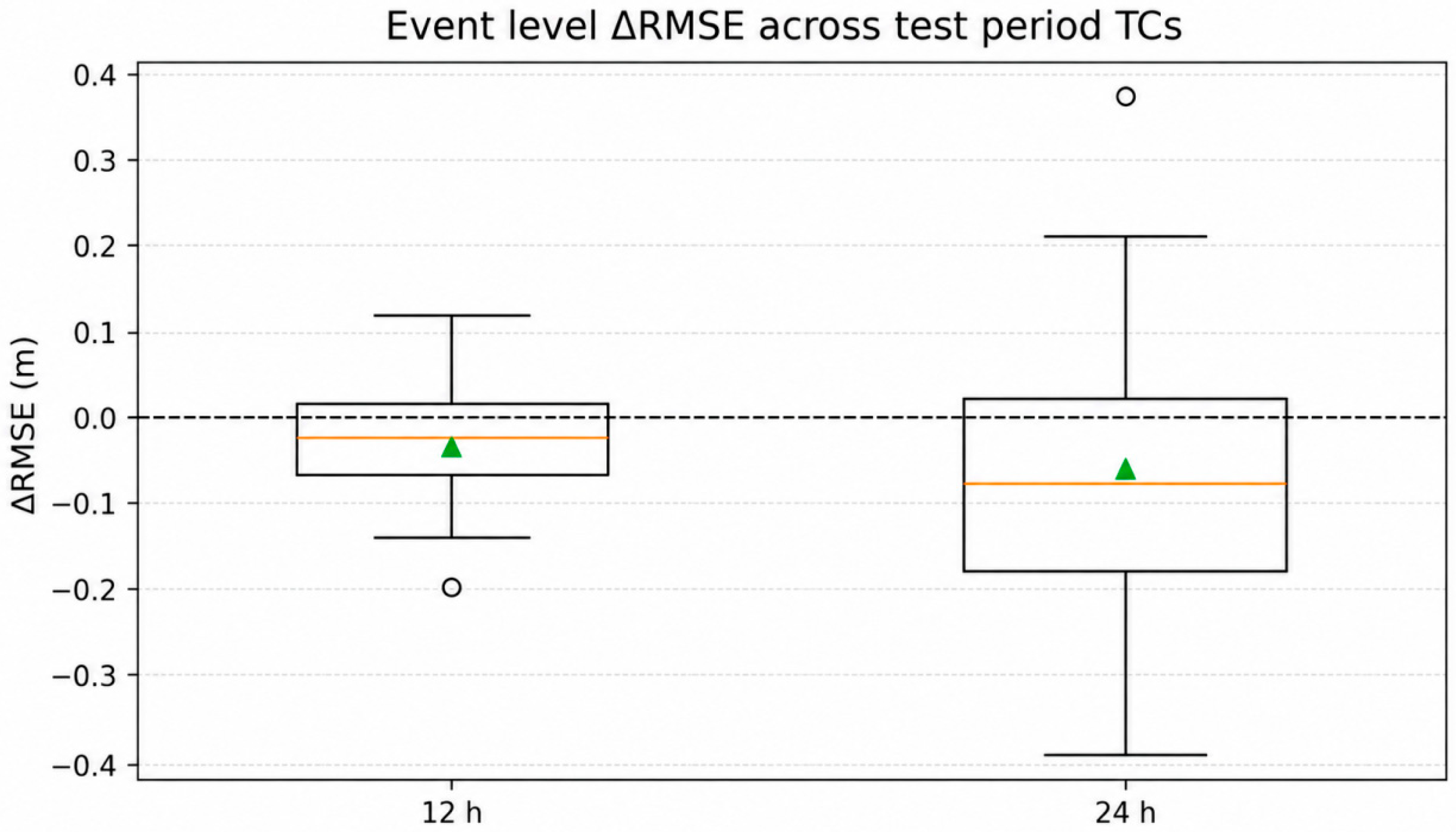
Sample-wise statistics can be dominated by storms with large sample counts. To avoid this bias and examine whether model improvements hold consistently across individual storm cases, we further conduct event-level performance evaluation for all 23 TC events in the test period. Each TC-associated sample is assigned to its nearest corresponding TC event within the forecast window, based on observed TC track records. RMSE differences between the MH-TCSeq2Seq and MH-TCSeq2Seq-FutureTC models are computed for each station event pair. The results are then aggregated by assigning equal weight to every TC storm, preventing storms with more hourly samples from dominating the outcome. The proportions of TC events and station event pairs for which FutureTC achieves lower RMSE values are also reported.

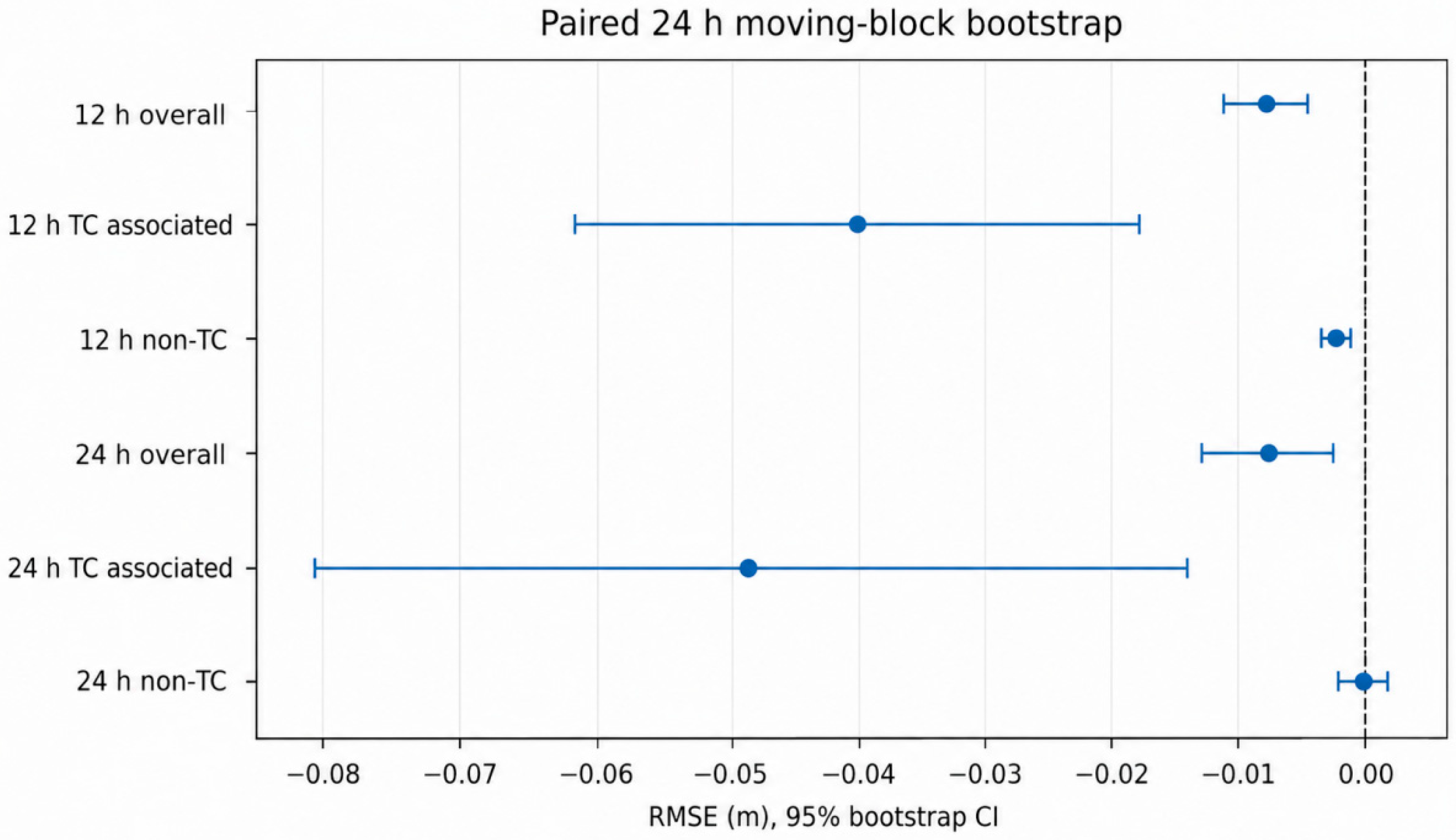
Hourly forecast samples show strong temporal autocorrelation, so standard statistical tests assuming independent samples are not suitable here. To quantify the uncertainty of skill differences between the MH-TCSeq2Seq and MH-TCSeq2Seq-FutureTC models, we adopt a paired circular moving-block bootstrap with 5000 replicates and a block length of 24 h [41]. An identical set of resampled time blocks is applied to outputs from both models for paired comparison. The evaluation metrics are first computed for each station and then equally averaged across the eight target stations. A complementary paired event cluster bootstrap is also performed by resampling complete TC events to evaluate the variability among storms.

2.6. SHAP-Based Feature Importance Analysis

Prior to interpretation using SHAP, forecast performance at the 12 and 24 h lead times is compared among all seven candidate models, namely, Persistence, MH-TCSeq2Seq, Q-BiGRU, TG-BiGRU, MH-TCSeq2Seq-FutureTC, Q-BiGRU-FutureTC, and TG-BiGRU-FutureTC, to identify the best performing model configurations. The best performing models with and without FutureTC inputs are selected for SHAP-based feature importance analysis. The analysis uses all TC-associated samples from the independent 2021–2023 test period, with the 12 h and 24 h outputs analyzed separately. SHAP provides a game theoretic framework for attributing individual model predictions to their corresponding input features and is widely used to interpret nonlinear machine-learning models [42].

SHAP values are calculated using GradientExplainer (SHAP version 0.49.1), with 50 SWH stratified training period samples per station used as the background set. Mean absolute SHAP values are first calculated within each station and then averaged equally across the eight stations to summarize the relative importance of local marine variables, historical TC descriptors, and future TC descriptors. Because some predictors within these groups are correlated, grouped permutation importance is further used as a complementary branch-level analysis [43]. For the local marine, historical TC, and FutureTC branches, all inputs within one branch are jointly permuted across TC-associated test samples within each station under the same random permutation index, while the other branches remain unchanged. The procedure is repeated 10 times for each branch, and branch importance is measured by the increase in RMSE relative to the original predictions.

3. Results and Discussion

This section integrates the principal results with their interpretation. Cross model comparisons are conducted at the common 12 and 24 h forecast horizons, whereas the additional 6 and 18 h results are used only to diagnose lead-time-dependent performance within the two MH-TCSeq2Seq variants. The analysis proceeds from overall model performance to TC-associated skill, station level variability, robustness, forecast track replacement, event scale behavior, SHAP attribution, and the main limitations.

3.1. Overall Performance and Model Configuration Effects

The overall forecasting skill is first assessed. As shown in

Table 3. Eight-station-averaged forecasting metrics for all models at the 12 and 24 h forecast horizons. Overall RMSE and overall R² are calculated over the full test dataset; RMSE_TC and RMSE_non-TC represent RMSE values computed exclusively over TC-affected and non-TC-affected samples, respectively.

Model	Overall RMSE (m)	Overall R2	RMSE_TC (m)	RMSE_non-TC (m)
Panel A. 12 h forecast
Persistence	0.262	0.698	0.518	0.231
Q-BiGRU	0.219	0.788	0.428	0.193
Q-BiGRU-FutureTC	0.223	0.776	0.478	0.191
TG-BiGRU	0.227	0.772	0.434	0.203
TG-BiGRU-FutureTC	0.233	0.760	0.470	0.204
MH-TCSeq2Seq	0.215	0.794	0.426	0.189
MH-TCSeq2Seq-FutureTC	0.207	0.808	0.385	0.187
Panel B. 24 h forecast
Persistence	0.389	0.364	0.825	0.331
Q-BiGRU	0.334	0.520	0.653	0.296
Q-BiGRU-FutureTC	0.356	0.455	0.812	0.294
TG-BiGRU	0.341	0.500	0.639	0.307
TG-BiGRU-FutureTC	0.353	0.476	0.690	0.314
MH-TCSeq2Seq	0.315	0.578	0.641	0.273
MH-TCSeq2Seq-FutureTC	0.307	0.599	0.594	0.273

Note: RMSE is computed for each station and then arithmetically averaged across the eight stations.

, MH-TCSeq2Seq-FutureTC achieves the lowest RMSE among all configurations at both horizons. At the 12 h horizon, its RMSE is 0.207 m, compared with 0.262 m for Persistence, 0.219 m for Q-BiGRU, 0.227 m for TG-BiGRU, and 0.215 m for MH-TCSeq2Seq. At the 24 h horizon, MH-TCSeq2Seq-FutureTC also obtains the lowest RMSE of 0.307 m, compared with 0.389, 0.334, 0.341, and 0.315 m for Persistence, Q-BiGRU, TG-BiGRU, and MH-TCSeq2Seq, respectively. The corresponding R² values show the same ranking, indicating that the FutureTC-augmented MH-TCSeq2Seq variant achieves the strongest overall deterministic forecasting skill for the 12 and 24 h horizons.

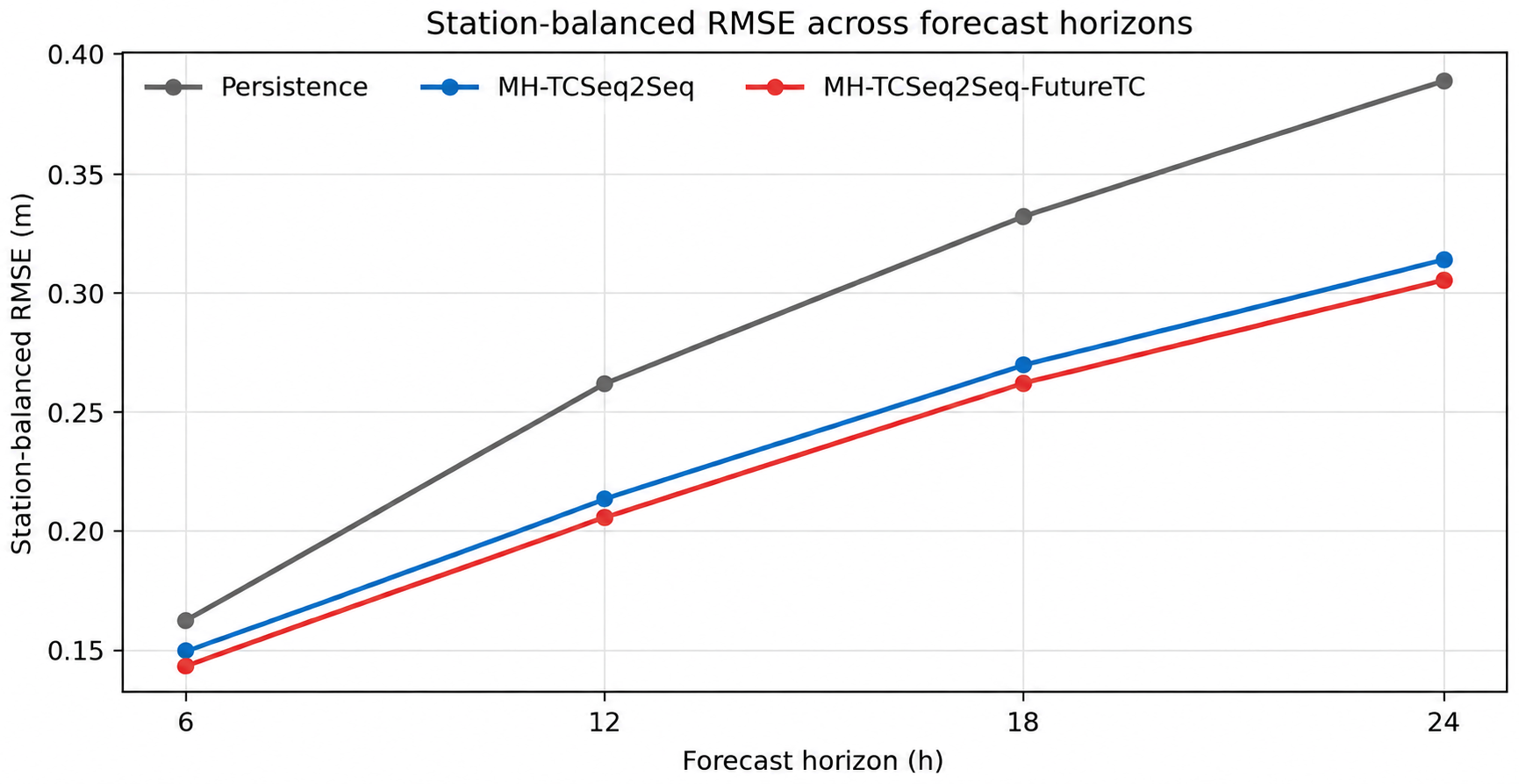
Figure 3 shows the lead time dependence of the station-balanced overall RMSE for Persistence and the two best performing MH-TCSeq2Seq configurations (with and without future TC inputs), which are available at all four forecast horizons. The RMSE increases progressively from 6 to 24 h for all three models, reflecting the increasing difficulty of longer-lead SWH forecasting. MH-TCSeq2Seq-FutureTC maintains a lower point estimate RMSE than MH-TCSeq2Seq at each horizon, indicating that the benefit of FutureTC is retained across the multi-horizon forecast range. Other recurrent baseline models are not included in Figure 3 to keep the plot focused; their full performance comparison is provided in Table 3.

Table 3 also shows that simply appending future TC predictors to the recurrent baseline models does not improve their overall forecast performance. Unlike MH-TCSeq2Seq, where future TC inputs yield clear performance gains, both Q-BiGRU-FutureTC and TG-BiGRU-FutureTC produce higher RMSEs than their corresponding non-FutureTC versions at the 12 and 24 h horizons. This contrast suggests that future TC descriptors are not automatically beneficial. Their usefulness depends on how TC trajectory information is integrated with local marine history, historical TC descriptors, and multi-horizon forecast constraints.

Under TC-associated conditions, all three learning-based base models substantially outperform Persistence. At the 12 h horizon, the RMSE_TC values of MH-TCSeq2Seq, Q-BiGRU, and TG-BiGRU are 0.426, 0.428, and 0.434 m, respectively, compared with 0.518 m for Persistence. At the 24 h horizon, TG-BiGRU achieves the lowest RMSE_TC of 0.639 m, followed closely by MH-TCSeq2Seq at 0.641 m and Q-BiGRU at 0.653 m, whereas Persistence reaches 0.825 m. The differences among the three learning-based models are small, and their ranking changes between the two forecast horizons. Thus, no single base architecture shows a consistent advantage under TC-associated conditions. Their consistent superiority over Persistence, particularly at 24 h, highlights the limitation of fixed value extrapolation for rapidly evolving storm-driven waves.

A clearer separation among the base models is observed for non-TC samples (Table 3). MH-TCSeq2Seq achieves the lowest RMSE_non-TC among the base architectures at both forecast horizons, with values of 0.189 m at 12 h and 0.273 m at 24 h. Importantly, introducing the FutureTC branch does not degrade the non-TC performance: RMSE_non-TC decreases slightly from 0.189 to 0.187 m at 12 h and remains essentially unchanged at 0.273 m at 24 h. This result indicates that FutureTC brings forecast improvements for TC-affected cases without imposing any performance penalty for ordinary non-TC conditions, which is highly desirable for operational forecasting. Given that TC-associated samples account for only approximately 7% of the test set, more pronounced FutureTC-related performance changes under TC conditions translate into relatively modest changes in overall RMSE.

A five-seed robustness analysis further evaluates model sensitivity to random initialization. Across seeds 42–46, MH-TCSeq2Seq-FutureTC yields lower mean station balanced overall RMSE than MH-TCSeq2Seq at both lead times, decreasing from 0.2150 ± 0.0032 to 0.2105 ± 0.0022 m at 12 h and from 0.3129 ± 0.0024 to 0.3068 ± 0.0019 m at 24 h. The corresponding mean ΔRMSE values are −0.0045 ± 0.0033 and −0.0061 ± 0.0039 m. Larger average reductions occur under TC-associated conditions, with ΔRMSE_TC of −0.0217 ± 0.0161 m at 12 h and −0.0372 ± 0.0268 m at 24 h, whereas non-TC differences remain small (−0.0017 ± 0.0021 and −0.0009 ± 0.0014 m). Lower overall and TC-associated RMSEs are obtained in four of the five seeds at both horizons, while seed 44 shows near neutral, slightly adverse differences. These results support an average FutureTC benefit, particularly under TC-associated conditions, while indicating that the magnitude of the incremental gain varies with random initialization rather than being guaranteed for every trained realization. Detailed seed wise results are provided in Table S2.

3.2. Spatial Variability of Forecast Errors Across Stations

Section 3.1 shows that MH-TCSeq2Seq-FutureTC achieves the optimal overall performance across all horizons, sample types and model groups. Among the base architectures, MH-TCSeq2Seq provides the best overall and non-TC performance, while the TC-associated rankings vary slightly between forecast horizons. To further explore the spatial heterogeneity of performance differences introduced by the FutureTC module, this section focuses exclusively on MH-TCSeq2Seq and its FutureTC-augmented variant, and

Table 4. Station-level overall and TC-associated RMSE of MH-TCSeq2Seq and MH-TCSeq2Seq-FutureTC at the 12 and 24 h forecast horizons. RMSE reduction refers to the relative percentage drop in RMSE after integrating the FutureTC branch.

Station	RMSE_MH (m)	RMSE_FutureTC (m)	Reduction (%)	RMSE_TC, MH (m)	RMSE_TC, FutureTC (m)	TC Reduction (%)	Overall Mean ERA5 Reference SWH (m)	TC-Associated Mean ERA5 Reference SWH (m)
Panel A. 12 h forecast
A	0.168	0.167	0.6	0.308	0.299	2.9	0.757	1.041
B	0.199	0.195	2.0	0.380	0.370	2.6	0.978	1.348
C	0.152	0.145	4.6	0.308	0.262	14.9	0.721	1.041
D	0.249	0.225	9.6	0.532	0.444	16.5	1.165	1.770
E	0.180	0.176	2.2	0.351	0.307	12.5	0.718	1.122
F	0.280	0.280	0.0	0.560	0.559	0.2	1.505	2.262
G	0.284	0.266	6.3	0.568	0.475	16.4	1.412	2.119
H	0.208	0.203	2.4	0.398	0.366	8.0	1.079	1.661
Mean	0.215	0.207	3.7	0.426	0.385	9.6	1.042	1.546
Panel B. 24 h forecast
A	0.235	0.233	0.9	0.462	0.470	−1.7	0.757	1.041
B	0.282	0.285	−1.1	0.561	0.587	−4.6	0.978	1.348
C	0.214	0.204	4.7	0.467	0.387	17.1	0.721	1.041
D	0.351	0.339	3.4	0.796	0.726	8.8	1.165	1.770
E	0.241	0.228	5.4	0.513	0.433	15.6	0.718	1.122
F	0.466	0.449	3.6	0.941	0.845	10.2	1.505	2.262
G	0.426	0.422	0.9	0.839	0.760	9.4	1.412	2.119
H	0.302	0.300	0.7	0.553	0.542	2.0	1.079	1.661
Mean	0.315	0.307	2.5	0.641	0.594	7.3	1.042	1.546

Note: For the mean row, RMSE values are arithmetic averages across eight stations. Reduction percentages in the mean row are calculated from these station-averaged RMSE values, not from averaging the per station percentage reduction values. MH = MH-TCSeq2Seq; FutureTC = MH-TCSeq2Seq-FutureTC.

compares their station-level forecasting metrics at the 12 and 24 h horizons.

For MH-TCSeq2Seq, the overall RMSE ranges from 0.152 m at Station C to 0.284 m at Station G for the 12 h forecast, and from 0.214 m at Station C to 0.466 m at Station F for the 24 h forecast. For MH-TCSeq2Seq-FutureTC, the corresponding RMSE ranges are 0.145–0.280 m and 0.204–0.449 m. Station C maintains the lowest forecast error at both horizons, whereas Stations F, G, and D generally show larger RMSE values. In terms of the ERA5 reference wave conditions, Station E records the lowest overall mean SWH, while Station F records the highest. Stations with larger mean SWH generally also have larger RMSEs. However, the improvement from FutureTC does not simply follow the local mean SWH. The wider RMSE range at the 24 h lead time indicates the stronger spatial heterogeneity of forecast error for longer prediction windows.

The performance gain brought by the FutureTC branch varies across stations and forecast horizons. The overall RMSE of MH-TCSeq2Seq drops for most station horizon pairs after integrating the FutureTC module. At 12 h, Station D shows the maximum reduction of the RMSE from 0.249 to 0.225 m (9.6%), followed by Station G with a 6.3% drop. At 24 h, Station F shows the largest absolute RMSE reduction, from 0.466 to 0.449 m, while Station E achieves the highest relative improvement of 5.4%. Stations C and D also show clear error declines. Slight performance degradation occurs only at Station B for the 24 h forecast, with RMSE rising by 0.003 m. These results confirm that FutureTC improves overall performance at most stations, although the magnitude of improvement differs spatially and temporally.

Station F is particularly notable. Despite having the highest mean SWH, FutureTC produces almost no improvement at 12 h, with overall and TC-associated RMSE reductions of only 0.0% and 0.2%, respectively. In contrast, at 24 h, FutureTC produces the largest absolute reductions, decreasing the overall RMSE by 0.017 m and the TC-associated RMSE by 0.096 m. These results show that the benefit of FutureTC at Station F becomes much more evident at the longer forecast horizon and is not simply related to the local wave magnitude.

FutureTC shows larger average error reductions under TC-associated conditions than for the overall sample. The eight-station-averaged TC-affected RMSE decreases by 9.6% at 12 h and 7.3% at 24 h, compared with overall RMSE reductions of 3.7% and 2.5%, respectively. At 12 h, the largest absolute TC-associated RMSE reductions occur at Stations G and D, reaching 0.093 and 0.088 m. At 24 h, Station F shows the maximum absolute RMSE reduction, while Station C achieves the largest relative improvement of 17.1%. However, the TC-associated RMSE increases slightly at Stations A and B at the 24 h lead time forecast. Overall, these results indicate that FutureTC provides greater benefits during TC-associated forecast windows, although the improvement is not spatially uniform.

3.3. Robustness Across TC Events and Temporal Dependence

In addition to the sample- and station-based results, we further examine model performance at the individual TC event level and quantify statistical uncertainty. The event-level analysis includes all 23 TCs during 2021–2023, resulting in 168 valid TC–station combinations with TC-associated samples at each forecast horizon. Compared with MH-TCSeq2Seq, MH-TCSeq2Seq-FutureTC reduces the RMSE by an average of 0.0274 m at 12 h and 0.0612 m at 24 h, with median reductions of 0.0223 and 0.0798 m. It achieves lower RMSEs for 15 of the 23 events (65.2%) at 12 h and 17 events (73.9%) at 24 h. At the TC–station level, a lower RMSE is obtained for 104 of 168 combinations at 12 h and 106 of 168 combinations at 24 h (Figure 4). These results show that the improvement is observed across many test events, although not every TC benefits from the additional future TC track information.

To further evaluate the uncertainty in these model differences, the temporal dependence among adjacent hourly predictions is also considered. Because these predictions are not independent, a paired moving-block bootstrap with 24 h blocks is applied (Figure 5). At 12 h, the overall ΔRMSE is −0.0074 m (95% CI: −0.0105 to −0.0041; p < 0.0002), while the TC-associated ΔRMSE is −0.0404 m (95% CI: −0.0602 to −0.0184; p = 0.0002). At 24 h, the corresponding differences are −0.0072 m (95% CI: −0.0124 to −0.0020; p = 0.0078) and −0.0478 m (95% CI: −0.0797 to −0.0126; p = 0.0058), respectively. In contrast, the 24 h non-TC difference is very small at −0.0001 m (95% CI: −0.0016 to 0.0013; p = 0.8618). A complementary TC event cluster bootstrap is also performed to assess the variation among individual TCs. It produces wider confidence intervals that cross zero at both horizons, indicating greater differences in model improvement among storms. Overall, the bootstrap results show lower average RMSEs for MH-TCSeq2Seq-FutureTC, particularly under TC-associated conditions, while the magnitude of the improvement varies among individual TC events.

3.4. Sensitivity to TC Forecast Track-Derived FutureTC Inputs

To assess whether the FutureTC branch remains effective when driven by operationally available TC forecast data, we carry out an input replacement experiment during the test period. The model retains the training configuration of MH-TCSeq2Seq-FutureTC, whereas the best track TC inputs for the forecast window are replaced with ATCF forecast track outputs issued at or before forecast initialization. Because the complete 24 h TC trajectory is available at initialization, using its trajectory descriptors for the 12 h forecast does not introduce future information leakage.

As shown in

Table 5. Overall and TC-associated RMSEs averaged over eight stations for MH, FutureTC, and MH-TCSeq2Seq-FutureATCF (FutureATCF) at the 12 and 24 h forecast horizons.

Horizon	FutureTC RMSE (m)	FutureATCF RMSE (m)	FutureTC RMSE_TC (m)	FutureATCF RMSE_TC (m)	MH RMSE_TC (m)
12 h	0.207	0.217	0.385	0.400	0.426
24 h	0.307	0.329	0.594	0.611	0.641

, the ATCF-driven configuration, denoted FutureATCF, obtains overall RMSE values of 0.217 m at 12 h and 0.329 m at 24 h. Its TC-associated RMSE values are 0.400 and 0.611 m, respectively. Compared with the best track-based FutureTC configuration, the TC-associated RMSE increases by 3.9% at 12 h and 2.9% at 24 h. This reduction in accuracy is consistent with uncertainties in forecast storm position, intensity, and timing, together with the input mismatch between best track-based training and ATCF-based testing. Nevertheless, compared with MH-TCSeq2Seq, FutureATCF reduces the TC-associated RMSE from 0.426 to 0.400 m at 12 h and from 0.641 to 0.611 m at 24 h, corresponding to improvements of 6.1% and 4.7%, respectively. These results indicate that operational forecast track information retains useful predictive value for TC-associated SWH forecasting.

3.5. Case Studies of Extreme TC Wave Events Along the Guangdong–Hong Kong Coast

Following the event robustness analysis in Section 3.3, three extreme TC cases are examined to illustrate event-scale forecast behavior. One event is selected from each year of the independent 2021–2023 test period based on the maximum ERA5 reference SWH along the Guangdong–Hong Kong coast. Table S3 ranks all TC events from 2021 to 2023 according to the peak SWH recorded across the eight coastal and offshore stations. The complete set of candidate TC–station event pairs used to construct this ranking is provided in Table S4. For each TC, the reported SWH corresponds to the maximum value recorded at any station during the event, and the station of event peak indicates where this maximum occurs.

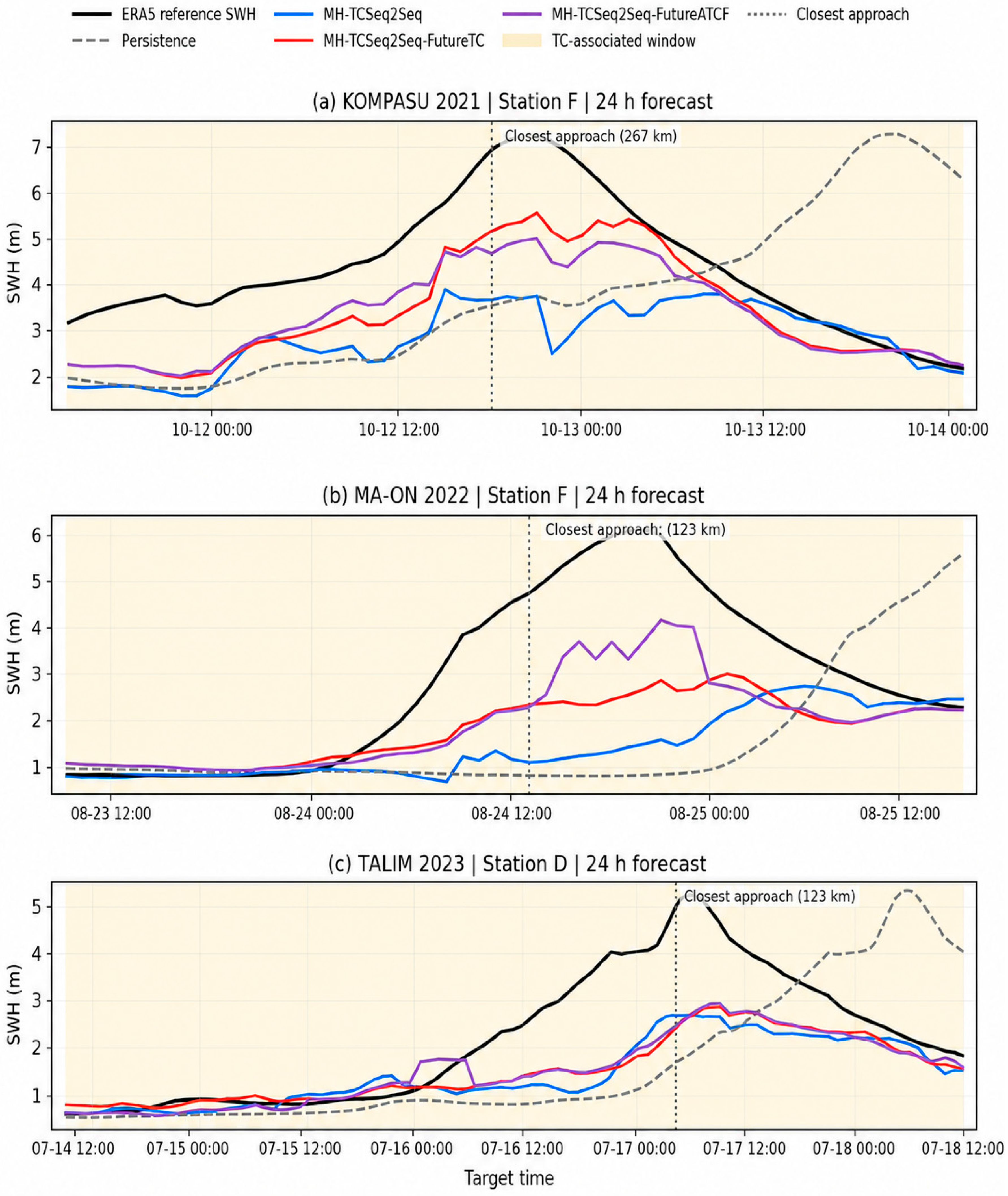
TC KOMPASU (2021) produces a maximum ERA5 reference SWH of 7.310 m at Station F; TC MA-ON (2022) produces a maximum SWH of 6.168 m at Station F; TC TALIM (2023) generates a maximum SWH of 5.341 m at Station D. Accordingly, we adopt KOMPASU 2021 (Station F), MA-ON 2022 (Station F), and TALIM 2023 (Station D) as representative cases to compare the forecast performance across all models.

Figure 6 presents time series comparisons of ERA5 reference SWH versus model forecasts for the 24 h lead time at the corresponding station of each TC: KOMPASU 2021 at Station F, MA-ON 2022 at Station F, and TALIM 2023 at Station D. For KOMPASU and MA-ON, MH-TCSeq2Seq-FutureTC and MH-TCSeq2Seq-FutureATCF reproduce the rise and fall of TC-driven waves more accurately than MH-TCSeq2Seq, even though both augmented models still underestimate the highest ERA5 wave peaks. In contrast, performance gains remain marginal for TALIM. Across the three case study panels (Figure 6), the ERA5 reference SWH peaks for Station F (two events) and Station D occur 2, 7, and 2 h after the closest approach of KOMPASU, MA-ON, and TALIM, respectively, indicating a short lag between storm proximity and the maximum local wave response. By contrast, forecast errors exhibit no consistent positioning relative to the wave peak. Such divergent improvements across the three TC cases demonstrate that the predictive benefit of the FutureTC module depends heavily on individual TC characteristics.

We further quantify model performance using case-specific RMSE values calculated for the three TC cases, as summarized in

Table 6. Case-wise RMSEs of Persistence, MH-TCSeq2Seq, MH-TCSeq2Seq-FutureTC and MH-TCSeq2Seq-FutureATCF for three representative extreme TC cases at the 24 h forecast horizon.

Case	Station	Persistence RMSE (m)	MH RMSE (m)	FutureTC RMSE (m)	FutureATCF RMSE (m)
KOMPASU 2021	F	2.640	1.945	1.161	1.231
MA-ON 2022	F	2.707	2.232	1.650	1.349
TALIM 2023	D	1.665	1.174	1.115	1.088

. Among all tested models, the Persistence baseline delivers the worst forecast accuracy. MH-TCSeq2Seq-FutureTC and MH-TCSeq2Seq-FutureATCF yield lower RMSEs than the baseline MH-TCSeq2Seq across all three events. For MA-ON and TALIM, MH-TCSeq2Seq-FutureATCF (driven by operational ATCF forecast tracks) outperforms MH-TCSeq2Seq-FutureTC (driven by reanalysis best tracks).

The most substantial error reduction appears for KOMPASU: RMSE declines from 1.945 m (MH-TCSeq2Seq) to 1.161 m (FutureTC) and 1.231 m (FutureATCF), corresponding to relative reductions of 40.3% and 36.7%, respectively. For MA-ON, RMSE drops from 2.232 m to 1.650 m and 1.349 m, with reductions of 26.1% and 39.6%. TALIM exhibits only modest improvements, with RMSE cut by 5.0% and 7.3% for FutureTC and FutureATCF respectively.

3.6. Feature Attribution During TC-Associated Periods

Global SHAP analysis is conducted using all TC-associated samples from the independent 2021–2023 test period to examine how MH-TCSeq2Seq and MH-TCSeq2Seq-FutureTC use their respective input predictors. Mean absolute SHAP values are first calculated separately for each station and forecast horizon and are then averaged across the eight stations, ensuring equal station-level weighting.

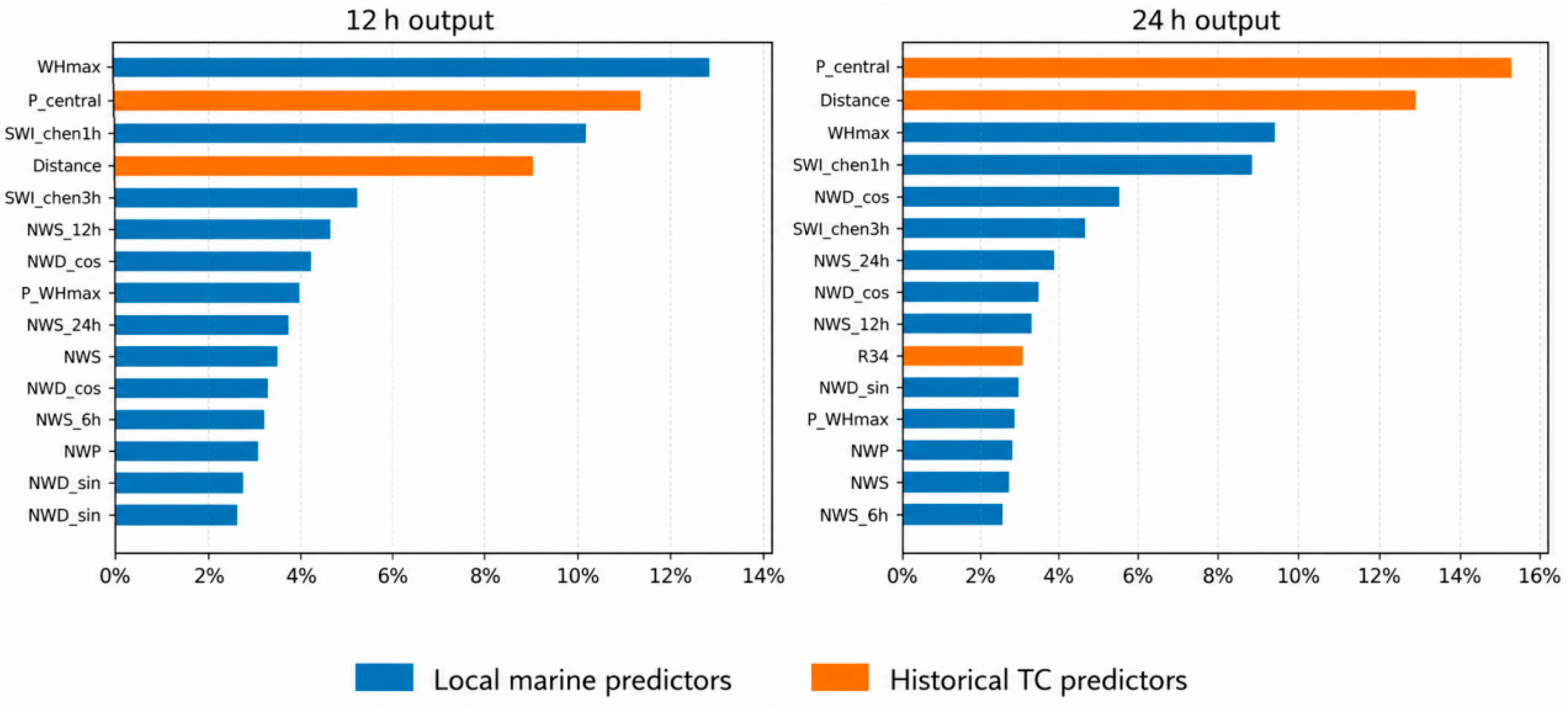
For the base MH-TCSeq2Seq model, the SHAP rankings indicate greater attribution to recent local marine conditions and historical TC information (Figure 7). At the 12 h lead time, WHmax, P_central, SWH_chan1h, and Distance are the leading predictors. At the 24 h lead time, P_central and Distance move to the top of the ranking, followed by WHmax and SWH_chan1h. This change suggests that historical TC intensity and TC–station geometry become relatively more influential as the forecast horizon increases.

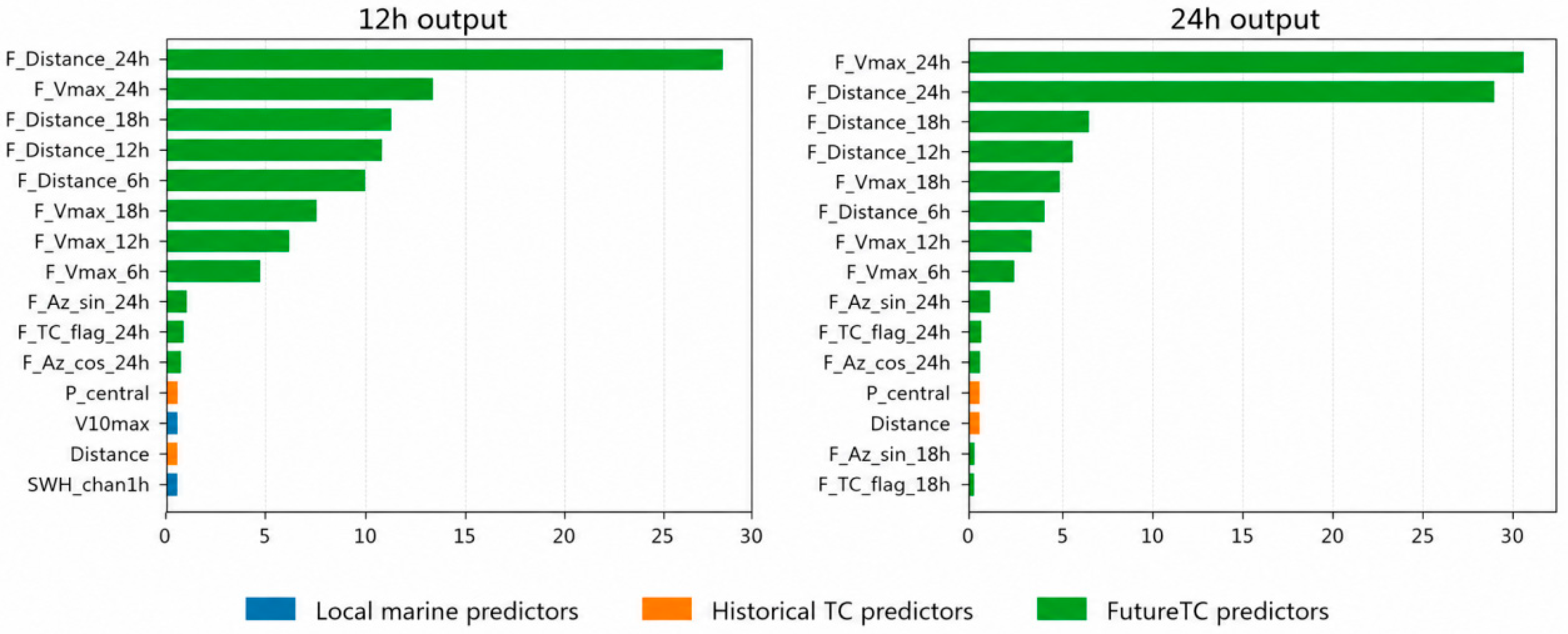
Once the FutureTC branch is integrated, future TC–station distance and intensity variables receive high SHAP attribution at both forecast horizons (Figure 8). At the 12 h forecast horizon, F_Distance_24h and F_Vmax_24h rank among the most influential inputs, together with future distance descriptors at shorter intermediate lead times. At the 24 h forecast horizon, F_Vmax_24h and F_Distance_24h rank first and second, followed by other future TC distance and intensity variables. These results indicate that MH-TCSeq2Seq-FutureTC relies strongly on information describing the expected evolution of storm proximity and intensity when generating TC period wave forecasts.

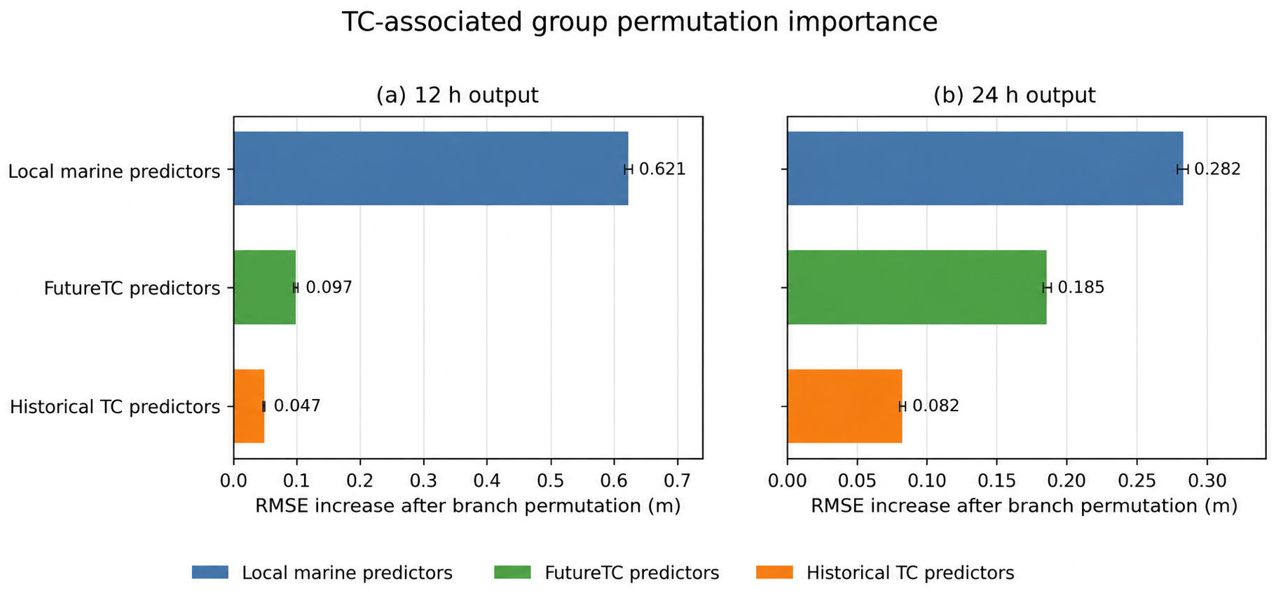
To corroborate the SHAP-based feature rankings shown in Figure 8, the group permutation analysis further examines the contribution of each input branch (Figure 9). Each branch is independently shuffled among TC-associated samples within the same station, while the other inputs remain unchanged. Permuting the local marine branch increases the RMSE by 0.621 m at 12 h and 0.282 m at 24 h, showing that recent marine conditions provide the main forecast basis. Permuting the FutureTC branch increases the RMSE by 0.097 and 0.185 m, respectively, indicating that Future TC information becomes more important at the longer forecast horizon. Historical TC permutation produces smaller increases of 0.047 and 0.082 m.

Overall, the two model configurations draw on distinct predictive information pathways. MH-TCSeq2Seq integrates recent wave conditions with historical TC intensity and location, whereas MH-TCSeq2Seq-FutureTC relies more strongly on forecasted future TC–station distance and intensity. This divergence in feature reliance aligns with the enhanced TC period forecast performance obtained by incorporating future TC trajectory inputs.

3.7. Limitations

Two limitations define the scope of these findings. First, the forecasts are evaluated against ERA5 reference SWH rather than independent in situ observations. The reported results therefore mainly reflect forecasting performance within the ERA5 reanalysis space. Independent validation using buoy or satellite altimeter observations would be needed to further assess the absolute accuracy of the forecasts under extreme TC conditions. Second, the main FutureTC experiment uses future TC descriptors derived retrospectively from best track records and therefore represents an idealized upper bound assessment. The FutureATCF experiment further evaluates the framework using forecast track information available at initialization, providing a more realistic assessment under forecast track uncertainty. The difference between the two configurations therefore reflects, at least in part, the influence of uncertainty in the predicted TC position, intensity, and timing.

The proposed framework is demonstrated only for the Guangdong–Hong Kong coast. However, the model architecture relies on region-independent predictors, TC–station distance, azimuth, intensity, and local marine variables, which can be derived for any coastal location with available TC track and wave data. Thus, the methodological framework is transferable to other TC-prone regions, though retraining with local data would be required. We leave this as a priority for future work.

4. Conclusions

This study presents a trajectory-informed multi-horizon Seq2Seq framework (MH-TCSeq2Seq) for 12 and 24 h SWH forecasting at eight coastal and offshore stations along the Guangdong–Hong Kong coast. Using separate encoding pathways and TC-aware information fusion, the baseline MH-TCSeq2Seq integrates local marine history and historical TC evolution. An enhanced variant further incorporates future TC trajectory descriptors within the forecast window, denoted MH-TCSeq2Seq-FutureTC. In the best track-based comparison, MH-TCSeq2Seq-FutureTC achieves the lowest overall RMSE, reaching 0.207 m at 12 h and 0.307 m at 24 h. Relative to MH-TCSeq2Seq, it reduces the TC-associated RMSE by 9.6% and 7.3%, respectively, while the non-TC performance changes only marginally. In contrast, adding the same future TC predictors to Q-BiGRU and TG-BiGRU degrades performance, indicating that the value of future TC information depends on the model architecture and how this information is integrated with historical inputs.

The improvement from FutureTC is not uniform across stations or individual storms, but an average benefit is evident across the broader test set. MH-TCSeq2Seq-FutureTC achieves lower RMSEs for most test period TCs and lower overall and TC-associated RMSE in four of the five random seed experiments at both forecast horizons. The paired moving-block bootstrap further supports lower average RMSE after accounting for temporal dependence, while the event cluster analysis indicates substantial storm-to-storm variability. SHAP and group permutation analyses further show strong model reliance on future TC information, particularly future TC–station distance and intensity-related descriptors. These results indicate that future TC trajectory information provides useful additional predictive information for multi-horizon SWH forecasting during TC-associated periods, although the magnitude of the improvement varies among storms and model initializations.

When retrospective best track inputs are replaced by the ATCF forecast guidance available at initialization, MH-TCSeq2Seq-FutureATCF still reduces the TC-associated RMSE by 6.1% at 12 h and 4.7% at 24 h relative to MH-TCSeq2Seq, although its performance remains below the idealized best track-based configuration. The best track results should therefore be interpreted as an upper bound assessment, while the FutureATCF experiment provides an operational-like sensitivity test indicating that forecast track information retains predictive value under more realistic input conditions. Further training with archived forecast guidance and independent validation against buoy or satellite altimeter observations are needed before extending these findings beyond ERA5 reanalysis space.

This work demonstrates two key contributions: a multi-source encoding architecture that separately processes local marine history, historical TC evolution and future TC trajectory information via TC-aware fusion. Predictive gains from future TC information are not universal but conditioned on model architecture and feature integration strategies. Overall, these findings indicate that future TC trajectory information can improve multi-horizon SWH forecasting under TC-associated conditions when appropriately integrated, underscoring the importance of tailored architecture design for utilizing TC information within forecast windows.