Fold-Reconstructed Sensitivity Priors and Structure-Preserving BP Neural Curves for Ducted Propeller Hydrodynamic Prediction

Abstract

Rapid surrogate prediction of ducted propeller performance is challenging when only a limited number of independent geometries are available and operating points belonging to the same geometry are strongly correlated. This study proposes a sensitivity-informed physics-regularized backpropagation neural network (SIPR-BP) for simultaneous prediction of the thrust coefficient K_T and the scaled torque coefficient 10K_Q. A CFD database comprising 20 Ka4-70-derived parameterized geometries, each evaluated at five advance ratios, provides 100 observations and 20 complete performance curves. The framework combines three main strategies. First, two-component multi-output partial least-squares (PLS) curve surrogates are reconstructed exclusively from the training geometries of each outer fold to generate leakage-controlled conditional Sobol gate priors. Second, the operating coordinate J is separated from geometric gating and represented by five ordered curve nodes, which guarantee non-increasing K_T and 10K_Q responses over the investigated interval. Third, training-only physics-consistency reliability weighting and a three-member ensemble improve robustness to locally irregular CFD responses and initialization variability. Under a ten-round geometry-grouped holdout protocol, SIPR-BP achieves a geometry-balanced MAPE of 2.65%, RMSE of 0.0112, MAE of 0.00911, and pooled R² of 0.951. When evaluated under the same outer partitions, a two-component PLS baseline yields a MAPE of 4.38%. Across the evaluated PLS, Extra Trees, GPR, and SVR baselines, SIPR-BP reduces geometry-balanced MAPE by approximately 39.6–79.2%. The results indicate that the proposed framework improves unseen-geometry prediction while preserving the prescribed response-curve structure.

1. Introduction

Ducted propellers are widely used in underwater vehicles and other high-load marine applications because they provide high thrust, favorable maneuverability, and improved resistance to cavitation at low advance ratios. Reliable prediction of their hydrodynamic performance is therefore fundamental to preliminary design and optimization. Considerable effort has been devoted to numerical methods that resolve the strong interaction between the propeller and the duct. Jin et al. [1] proposed a coupled Boundary Element Method-Reynolds-Averaged Navier–Stokes (BEM-RANS) approach, while Li et al. [2] developed a parametric optimization framework integrating geometric modeling, multi-objective genetic algorithms, and experimental validation. RANS-based Computational Fluid Dynamics (CFD) has also been applied to oblique flow [3], steady and unsteady propeller operation [4], wave-induced performance variation [5], cavitating equalizing ducts [6], hull-motion-induced excitation [7], and ducted propeller design and testing [8]. Collectively, these studies demonstrate the fidelity of CFD for resolving complex blade-duct interactions, but they also expose the computational burden that limits repeated use in iterative design.

Data-driven surrogates offer a practical route to replacing repeated CFD evaluations during extensive parametric exploration. Valcic and Dejhalla [9] used neural networks to estimate the open-water characteristics of Wageningen ducted propellers, and Shora et al. [10] combined CFD with an artificial neural network to predict thrust, torque, and cavitation volume under variations in pitch ratio, rake angle, skew angle, advance ratio, and cavitation number. Dong et al. [11] further demonstrated the value of data-driven optimization in multidisciplinary underwater-vehicle design. Related studies have mapped propeller geometry and operating conditions to hydrodynamic responses using experimental neural models [12,13], self-organizing maps and multivariate analysis [14], multitask artificial neural networks (ANNs) for complete coefficient curves [15], cross-series machine learning design [16], and multi-fidelity transfer learning [17]. These developments establish the promise of learning-based propeller surrogates, but they also highlight the need for evaluation protocols and model structures that remain credible when only a small number of independent geometries is available.

Among available neural architectures, the backpropagation (BP) network remains attractive for small-sample engineering surrogates because it combines a compact structure, mature optimization procedures, and strong nonlinear approximation capability. BP-based models have supported energy-saving optimization of propeller boss cap fins [18], identification of unmanned surface vehicle dynamics [19], prediction of AU-type propeller open-water performance from CFD data [20], and neural-fuzzy motion control of biomimetic robotic fish [21]. These applications confirm that BP networks can provide computationally efficient mappings when numerical or experimental databases are limited; however, their effectiveness depends strongly on how prior engineering knowledge and validation structures are introduced.

Three methodological limitations remain particularly important for limited-geometry ducted propeller prediction. First, treating operating points from the same geometry as independent samples can transfer geometry-specific information between training and test sets and thereby overstate generalization. Second, directly mixing the operating coordinate with geometric descriptors obscures their distinct roles: the former locates a point along a performance curve, whereas the latter governs curve-to-curve variation. Third, unconstrained black-box regressors do not guarantee physically expected response directions and may be sensitive to locally irregular CFD observations or random initialization. Existing BP surrogates rarely address these three issues within a single leakage-controlled framework. A model that coordinates geometry-level validation, sensitivity-guided feature allocation, and structural curve constraints is therefore needed.

The standard Ka4-70 propeller operating with a No. 19A duct provides the reference configuration for the present study. The standard Ka4-70 blade is a fixed-pitch design with a constant radial pitch ratio. In the present database, however, this standard configuration is used only as the reference and CFD benchmark: pitch, skew, rake, and blade thickness are deliberately parameterized to construct modified Ka4-70-derived geometries. These sampled designs should therefore not be interpreted as standard members of the Ka series. The distinction is important because the objective of the present work is not to reproduce the complete Ka-series catalogue, but to evaluate geometry-level surrogate prediction over a controlled four-dimensional modification space. Pitch is intentionally retained as a principal design degree of freedom because it strongly influences thrust and torque; the conditional sensitivity analysis in Section 5 subsequently confirms its dominant contribution within the sampled bounds.

To close these gaps, this study introduces a sensitivity-informed physics-regularized backpropagation neural network (SIPR-BP) that couples fold-reconstructed sensitivity priors with structure-preserving performance curves. Its distinctive contribution is the coordinated architecture and information flow rather than an isolated modification to a conventional BP network. Specifically, (1) 20 independently parameterized Ka4-70-derived geometries are simulated at five advance-ratio conditions and retained as complete geometry curves; (2) a surrogate-assisted conditional Sobol workflow separates the operating coordinate J from geometric sensitivity, validates two-component multi-output PLS curve surrogates by strict leave-one-geometry-out prediction, and reconstructs output-specific gate priors exclusively inside every outer training fold; (3) five ordered nodes for K_T and 10K_Q impose a non-increasing curve structure as J increases; (4) training-only physics-consistency reliability weights provide robust soft reweighting without deleting observations; and (5) a three-member ensemble and a balanced geometry-group holdout protocol jointly support ablation, benchmark, paired statistical, and dense-grid physical-consistency analyses. This integrated design directly targets geometry-level generalization while preventing held-out geometries from influencing any data-dependent component of the modeling pipeline.

2. Parametric Geometric Model of the Ducted Propeller

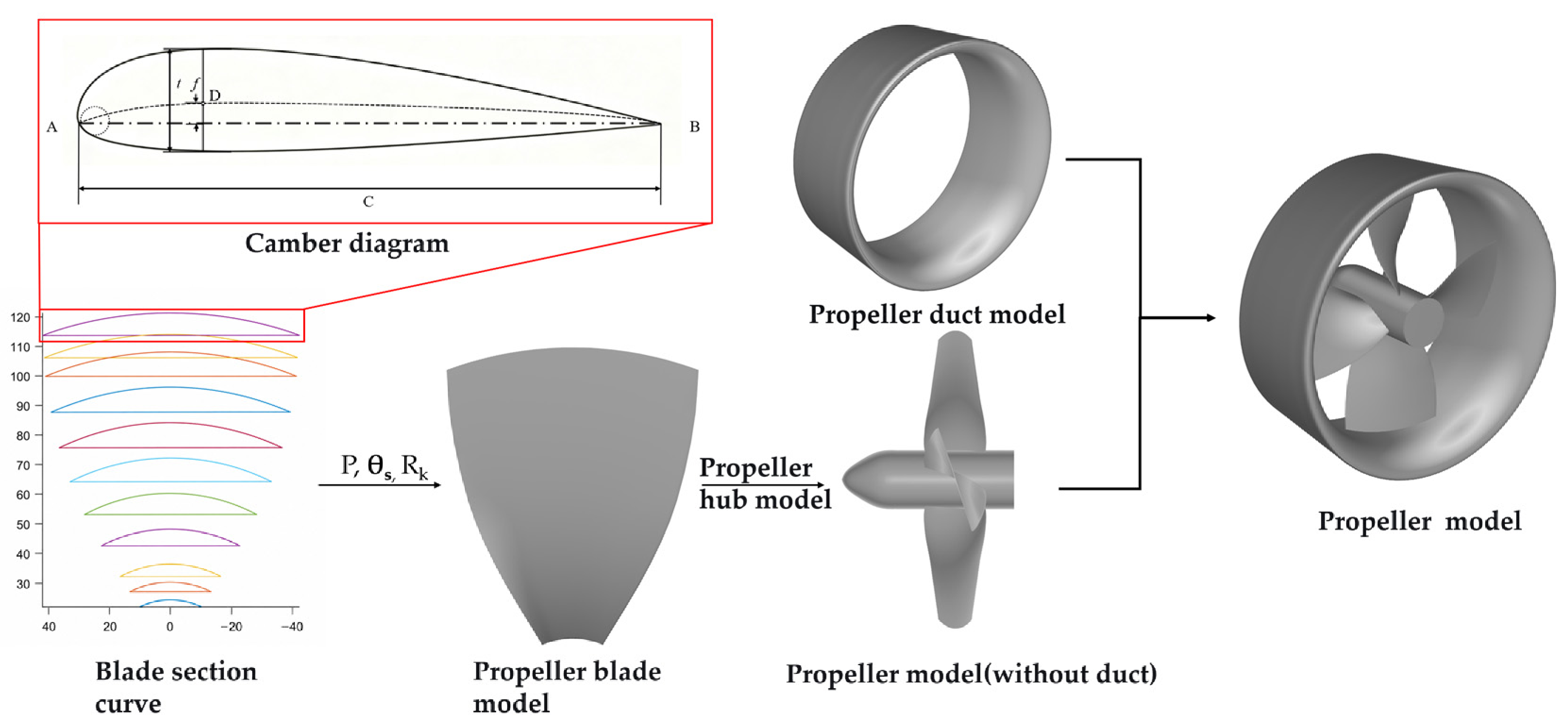
Two geometric definitions are distinguished throughout this study. First, the standard four-bladed Ka4-70 propeller with a No. 19A duct is used as the reference configuration and for CFD benchmark assessment. Second, the machine learning database is constructed from 20 Ka4-70-derived parameterized geometries in which selected blade descriptors are deliberately varied. The propeller diameter is D = 240 mm. Figure 1 summarizes the modeling workflow, and the following subsections define the standard reference geometry and the parameterized blade-generation procedure.

2.1. Blade Model and Parameters

The standard Ka4-70 propeller is adopted as both the reference geometry and the propeller used for CFD benchmark assessment. The propeller has four blades, an expanded-area ratio A_E/A₀ = 0.70, and a constant radial pitch ratio P/D = 1.0. Its radial chord and thickness distributions are reconstructed from the standard Ka-series geometric data reported by Sheng and Liu [22], as summarized in

Table 1. Principal radial parameters of the standard Ka4-70 reference propeller.

r/R	b/D	P/D	θs	Rk	t/D
0.20	0.2314	1.000	0	0	0.0400
0.30	0.2639	1.000	0	0	0.0352
0.40	0.2935	1.000	0	0	0.0300
0.50	0.3205	1.000	0	0	0.0245
0.60	0.3446	1.000	0	0	0.0190
0.70	0.3648	1.000	0	0	0.0138
0.80	0.3793	1.000	0	0	0.0092
0.90	0.3882	1.000	0	0	0.0061
1.00	0.3890	1.000	0	0	0.0050

.

The two-dimensional blade sections of the standard Ka4-70 propeller are defined separately using the published Ka-series sectional ordinates in the same reference. These data specify the blade-back and blade-face ordinates at prescribed chordwise positions relative to the maximum-thickness location, with the ordinates expressed as percentages of the local maximum blade thickness. The complete published geometric data used to define the standard Ka4-70 benchmark blade, including the radial dimensional relations and the blade-back and blade-face sectional ordinates, are provided in Supplementary Tables S1–S3. Thus, the standard Ka4-70 sectional definition is kept distinct from the modified NACA 66 sectional construction subsequently used for the 20 parameterized database geometries.

For the Ka4-70 configuration, Z = 4 and A_E/A₀ = 0.70. Following the standard Ka-series definition in Ref. [22], the reference chord length at r/R = 0.6 is calculated from

$${\displaystyle \frac{b_{0.6}}{D}}=1.969{\displaystyle \frac{1}{Z}}{\displaystyle \frac{A_E}{A_0}}=0.344575$$

(1)

The chord lengths at the remaining radial stations are obtained from the corresponding percentages of the 0.6R section length reported in Ref. [22]. The maximum-thickness ratios in Table 1 are taken directly from the same standard Ka-series definition.

In contrast to the standard Ka4-70 benchmark geometry described above, the 20 parameterized database geometries are generated separately from 11 radial sectional parameter records. Their two-dimensional sections use a modified NACA 66 thickness distribution combined with an a = 0.8 camber-line distribution. The geometry generator uses 27 normalized chordwise ordinates, which are provided in Supplementary Table S4.

2.1.1. Generation of the Two-Dimensional Surface Points of the Parameterized Blade Section

For each radial station, the dimensional radius r, chord b, pitch P, maximum thickness t_max, and maximum camber f_max are obtained from the corresponding nondimensional geometric parameters as

$$\begin{array}{c}r=\left({\displaystyle \frac{r}{R}}\right){\displaystyle \frac{D}{2}},\hspace{1em}b=\left({\displaystyle \frac{b}{D}}\right)D,\hspace{1em}P=\left({\displaystyle \frac{P}{D}}\right)D,\\ t_{\mathit{max}}=\left({\displaystyle \frac{t}{D}}\right)D,\hspace{1em}{f}_{\mathit{max}}=\left({\displaystyle \frac{f}{b}}\right)b.\end{array}$$

(2)

Let $\overline{x}$, $\overline{t}$, and $\overline{f}$ denote the normalized chordwise position, normalized thickness ordinate, and normalized camber ordinate, respectively. The corresponding dimensional camber-line coordinate, local thickness, and camber ordinate are

$$x_c=\overline{x}b, t=\overline{t}{t}_{\mathit{max}}, y_c=\overline{f}{f}_{\mathit{max}}.$$

(3)

The local inclination of the camber line is defined as

$$\gamma =\arctan \left({\displaystyle \frac{d{y}_c}{d{x}_c}}\right)$$

(4)

Using the local camber-line inclination, the upper- and lower-surface coordinates are reconstructed as

$$\left.\begin{array}{l}{x}_u=x_c-{\displaystyle \frac{t}{2}}\sin \gamma \\ y_u=y_c-{\displaystyle \frac{t}{2}}\sin \gamma \end{array}\right\}\left.\begin{array}{l}\hspace{1em}\hspace{1em}\hspace{1em}{x}_l=x_c-{\displaystyle \frac{t}{2}}\sin \gamma \\ \hspace{1em}\hspace{1em}\hspace{1em}{y}_l=y_c-{\displaystyle \frac{t}{2}}\sin \gamma \end{array}\right\}$$

(5)

2.1.2. Transformation from Two-Dimensional Coordinates to Three-Dimensional Spatial Coordinates

The local pitch angle at each radial station is calculated as

$$\theta =\arctan ({\displaystyle \frac{P}{2\pi r}})$$

(6)

where P is the local pitch and r is the dimensional radius of the corresponding radial station.

The sectional coordinates are mapped to the global three-dimensional blade system using the local pitch angle, together with the station-specific skew and rake values. The geometric construction naturally employs cylindrical relations: each radial section is positioned at its prescribed radius and wrapped onto the corresponding coaxial cylindrical surface, while the angular displacement accounts for skew and the axial displacement accounts for pitch and rake. The resulting point coordinates are then expressed in the global Cartesian system (x,y,z) because these coordinates can be passed directly to the CAD environment for point, spline, surface, and solid construction. Thus, cylindrical coordinates are used conceptually in the geometric mapping, whereas Cartesian coordinates are retained as the final CAD representation. This choice does not alter the prescribed blade geometry but simplifies the interface between the analytical parameterization and the subsequent solid-modeling operations. The complete 11-station chord, pitch, skew, rake, thickness, and camber distributions used to generate the 20 parameterized geometries are provided in Supplementary Table S5.

$$\left.\begin{array}{l}x=-i_G-r{\theta }_s\tan \theta +(0.5c-x_c)\sin \theta +(y_c\pm 0.5t\cos \gamma )\cos \theta \\ y=r\sin \left[{\theta }_s-{\displaystyle \frac{(0.5c-x_c)\cos \theta -(y_c\pm 0.5t\cos \gamma )\sin \theta }{r}}\right]\\ z=r\cos \left[{\theta }_s-{\displaystyle \frac{(0.5c-x_c)\cos \theta -(y_c\pm 0.5t\cos \gamma )\sin \theta }{r}}\right]\end{array}\right\}$$

(7)

The parameter-to-geometry conversion is implemented using a custom script written by python 3.13 and executed within the developer environment of the commercial CAD package Siemens NX 2412. The custom script evaluates the sectional geometry and coordinate-transformation equations for all prescribed radial stations and transfers the resulting Cartesian point sets to NX, where the corresponding curves, blade surfaces, and solid geometry are constructed. Therefore, the geometric parameterization and coordinate generation are custom-developed, whereas the CAD construction and solid-modeling operations are performed within Siemens NX 2412. The completed geometry is exported in Parasolid format for assembly, mesh generation, and subsequent CFD analysis.

2.2. Duct and Hub Model and Parameters

The standard No. 19A section is used as the duct profile, with its ordinate definition taken from Sheng and Liu [22]. A uniform 1 mm tip clearance is maintained between the blade tips and the duct’s inner wall. The duct length is 120 mm, corresponding to c/D = 0.5. The inlet and outlet contours and the duct installation angle follow the standard No. 19A definition. The three-dimensional duct is generated by revolving the section curve about the propeller axis in NX.

The hub comprises a cylindrical main body and a streamlined tail cap. Its diameter ratio is dh/D = 0.2, giving a hub diameter of 48 mm. The streamlined cap provides a smooth fairing transition, limits separation near the hub, and connects the blades continuously to the hub body.

After the blade, duct, and hub are generated, Boolean operations assemble them into the complete ducted propeller geometry. The resulting solid is exported in Parasolid format and used directly as the geometric input for meshing and CFD calculations.

3. Sensitivity-Informed Physics-Regularized Backpropagation Neural Network (SIPR-BP)

3.1. Overall Framework

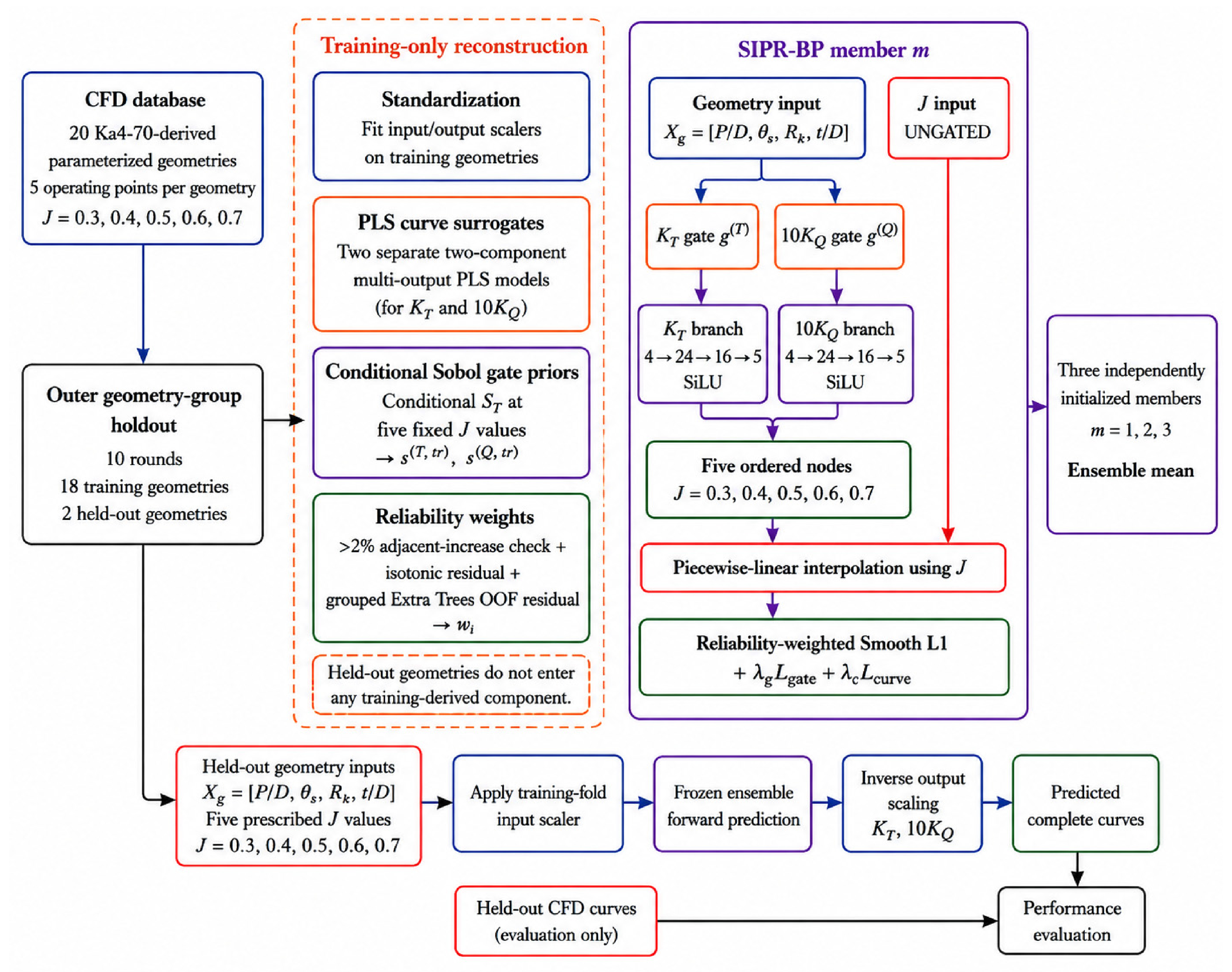
SIPR-BP integrates five mutually reinforcing components: training-subset standardization, output-specific Sobol sensitivity gating of the geometric variables, structurally monotonic performance curves along the advance ratio J, physics-consistency reliability-based soft weighting, and a three-member deep ensemble. The innovation lies in the fold-wise coordination of these components: sensitivity information allocates geometric influence without using test data, ordered nodes encode the expected curve direction, reliability weighting limits the effect of locally irregular training observations, and ensemble averaging suppresses initialization variability. Figure 2 shows the architecture and the complete training information flow.

3.2. Input and Output Variables and Standardization

The model input is the five-dimensional vector X = [J, P/D, θ_s, R_k, t/D], and the output is Y = [K_T, 10K_Q]. The angular variables θ_s and R_k are entered in degrees. In every outer validation round, the input and output scalers are fitted exclusively to the current training geometries and then applied unchanged to the corresponding training and test subsets. For any input or output variable v, the transformation is

$$\widetilde{v_i}={\displaystyle \frac{v_i-{\mu }_v^{tr}}{{\sigma }_v^{tr}}}$$

(8)

where v_i is the value of variable v for sample i; ${\mu }_v^{tr}$ and ${\sigma }_v^{tr}$ are the mean and standard deviation, respectively, estimated from the current outer-training subset; and ${\tilde{v}}_i$ is the standardized value. The superscript tr explicitly denotes that no held-out geometry contributes to the preprocessing statistics.

The physical torque coefficient retains its conventional definition. A constant factor of 10 is applied only to the learning target so that its numerical scale is comparable to that of K_T:

$$K_Q={\displaystyle \frac{Q}{\rho n^2{D}^5}},\hspace{1em}10K_Q={\displaystyle \frac{10Q}{\rho n^2{D}^5}}$$

(9)

where Q is the propeller torque, ρ the fluid density, n the rotational speed in revolutions per second, and D the propeller diameter. The scaled quantity 10K_Q is used consistently in training, prediction, figures, and tables. Because multiplication by a positive constant does not alter variance-based indices, K_Q and 10K_Q have identical conditional Sobol indices at the same fixed J.

3.3. Output-Specific Sensitivity Gating for Geometric Variables

The advance ratio J identifies the operating location on an ordered performance curve and is therefore deliberately excluded from gating. Instead, the geometric vector x_g = [P/D, θ_s, R_k, t/D] is processed through a separate positive gate for each output branch. At the beginning of every outer validation round, a two-component multi-output PLS curve surrogate is reconstructed using only the 18 training geometries. Conditional total-effect indices are evaluated at the five fixed J levels and aggregated using output-variance weights to initialize the four geometry-gate proportions. This fold-reconstructed design prevents both held-out geometries and their operating rows from influencing the sensitivity prior:

$${g_j}^{(o)}={\displaystyle \frac{\mathrm{softplus}({a_j}^{(o)})+\epsilon }{\frac{1}{p}{\displaystyle \sum _{r=1}^p[\mathrm{softplus}({a_r}^{(o)})+\epsilon ]}}}$$

(10)

where o denotes the thrust branch T or torque branch Q; j indexes the p = 4 geometric variables; a_j^(o) is the trainable raw gating parameter; ε = 10⁻⁶ prevents a zero gate; softplus(·) enforces positivity; and g_j^(o) is the normalized gate applied to geometric variable j in output branch o.

A weak prior loss transfers the fold-specific Sobol ranking to the normalized gate proportions while preserving their ability to adapt to the prediction objective:

$$L_{gate}={\displaystyle \frac{1}{2}}{\displaystyle \sum _{o\in \left\{T,Q\right\}}\mathrm{MSE}\left(\frac{g^{(o)}}{{\displaystyle {\sum }_j{g_j}^{(o)}}},\frac{s^{(o)}}{{\displaystyle {\sum }_j{s_j}^{(o)}}}\right)}$$

(11)

where g^(o) is the learned geometry-gate vector and s(o, tr) is the fold-specific normalized vector of variance-weighted conditional total-effect indices for output branch o. MSE(·,·) denotes the mean squared difference. The superscript tr emphasizes that the prior is independently reconstructed from the current outer-training geometries rather than transferred from the full dataset.

3.4. Dual-Branch Monotonic Performance-Curve Architecture

K_T and 10K_Q are represented by two independent geometry-conditioned curve branches. Each branch uses a 4 → 24 → 16 → 5 feedforward architecture with SiLU activations and predicts one unconstrained baseline parameter, together with four raw decrement parameters. Transforming the decrements to non-negative values and cumulatively subtracting them produces five intrinsically ordered nodes:

$${{\delta }_k}^{(o)}=\mathrm{softplus}({d_k}^{(o)})\ge 0{y_0}^{(o)}=b^{(o)}$$

(12)

$${y_k}^{(o)}=b^{(o)}-{\displaystyle \sum _{r=1}^k{{\delta }_r}^{(o)}}, k = 1, \dots , 4$$

(13)

where o denotes the output branch; b^(o) is the baseline node; ${d_k}^{(o)}$ is the k-th raw decrement; ${{\delta }_k}^{(o)}$ is its non-negative softplus transform; and ${y_k}^{(o)}$ is the node value at operating point k. Because every ${{\delta }_k}^{(o)}$ is non-negative, the node sequence cannot increase with k.

The five nodes are anchored at J = 0.3, 0.4, 0.5, 0.6, and 0.7. For any J within this interval, the normalized position and the interpolation coefficient between adjacent nodes are defined as follows:

$$\left.\begin{array}{l}{J}_k=0.3+0.1k,\\ \xi =\mathrm{clip}({\displaystyle \frac{J-0.3}{0.4}},0.1),\\ k=\min (\mathrm{floor}(4\xi ),3),\\ \alpha =4\xi -k\end{array}\right\}$$

(14)

$${\hat{y}}^{(o)}(J)=(1-\alpha ){y_k}^{(o)}+\alpha y_{k+1}^{(o)}$$

(15)

where J_k is the k-th node location; ξ is the clipped normalized advance ratio; k selects the left node of the active interval; α is the local interpolation fraction; and ${\hat{y}}^{(o)}$(J) is the predicted K_T or 10K_Q. Piecewise-linear interpolation between ordered nodes guarantees a non-increasing response for every J over 0.3 ≤ J ≤ 0.7, rather than merely penalizing violations at sampled points [23].

3.5. Physics-Consistency Reliability-Based Soft Weighting

The reliability module is reconstructed independently within the training subset of every outer validation round, so test geometries never participate in weight estimation. For each training geometry, the K_T and 10K_Q sequences are inspected in ascending J order. In the complete CFD database, 3 of the 20 geometries contain at least one adjacent increase exceeding the adopted 2% tolerance. In total, six output-specific adjacent transitions exceed the threshold and involve eight distinct geometry–operating-condition observations. All corresponding CFD solutions were rechecked and retained. Because the available evidence does not permit the local increases to be attributed uniquely to discretization-related variability or to genuine local hydrodynamic behavior, they are treated as valid but trend-inconsistent observations rather than as erroneous data. Local increases not exceeding 2%, residuals from a non-increasing isotonic projection, and geometry-grouped Extra Trees reference residuals are combined into the non-negative inconsistency score s_i. The resulting training-only soft reweighting reduces the influence of locally irregular observations while retaining every sample [24]. The continuous reliability weight is

$$w_i=\max (w_{\mathit{min}},e^{-s_i}),\hspace{1em}{w}_{\mathit{min}}=0.05$$

(16)

where s_i ≥ 0 is the inconsistency score of training sample i, w_i is its reliability weight, and w_min = 0.05 is the retained lower bound. Thus, s_i = 0 gives full weight, increasingly inconsistent observations are down-weighted smoothly, and no sample is removed. The weights do not alter the target values, and all outer-test observations remain unweighted during evaluation.

3.6. Loss Function and Training

Data fitting is performed on the standardized output scale using a reliability-weighted Smooth L1 loss. For a residual e, the Smooth L1 function is defined as

$$l_{\beta }(e)=\left\{\begin{array}{l}{\displaystyle \frac{e^2}{2\beta }},\hspace{1em}\hspace{1em}\left|e\right|<\beta \\ \left|e\right|-{\displaystyle \frac{\beta }{2}}, \left|e\right|\ge \beta \end{array}\right. \hspace{1em}\beta =0.15$$

(17)

where e is the standardized prediction residual and β = 0.15 is the transition threshold. The quadratic region promotes accurate fitting of small residuals, whereas the linear-growth region limits the leverage of large residuals.

The two output losses are first averaged at the sample level and then aggregated using the reliability weights:

$$L_{\mathit{data}}={\displaystyle \frac{{\displaystyle {\sum }_{i=1}^N{w}_i\left[\frac{1}{2}{\displaystyle \sum o\in \left\{T,Q\right\}{l}_{\beta }({\widehat{z_i}}^{(o)}-{z_i}^{(o)})}\right]}}{{\displaystyle {\sum }_{i=1}^N{w}_i}}}$$

(18)

where N is the number of training samples; z_i^(o) and ${{\hat{z}}_i}^{(o)}$ are the standardized target and prediction for sample i and output o, respectively; and w_i is the physics-consistency reliability weight.

Curve regularization is applied only to the final three decrement parameters of each output branch:

$$L_{\mathit{curve}}={\displaystyle \frac{1}{2}}\left[{\mathrm{mean}}_{i,k=2,3,4}{({{\delta }_{i,k}}^{(T)})}^2+{\mathrm{mean}}_{i,k=2,3,4}{({{\delta }_{i,k}}^{(Q)})}^2\right]$$

(19)

where δ_i,k^(T) and δ_i,k^(Q) are the k-th non-negative decrements predicted for sample i in the K_T and 10K_Q branches, respectively. The complete training objective is

$$L=L_{\mathit{data}}+{\lambda }_g{L}_{\mathit{gate}}+{\lambda }_c{L}_{\mathit{curve}},\hspace{1em}{\lambda }_g={10}^{-2}, {\lambda }_c={10}^{-5}$$

(20)

where L_data is the reliability-weighted fitting loss, L_gate is the conditional-Sobol gate-prior loss, L_curve is the decrement regularization term, and λ_g and λ_c are the corresponding weights. Importantly, monotonicity is guaranteed by the ordered-node construction rather than by L_curve. Optimization uses AdamW, cosine-annealed learning rates, and gradient clipping. A0–A2 use unit training weights, whereas A3 and SIPR-BP use the fold-reconstructed reliability weights.

3.7. Three-Member Deep Ensemble

The final SIPR-BP is an ensemble of three reliability-weighted monotonic networks trained on identical fold-specific information but initialized independently. Their arithmetic mean defines the final prediction:

$$\widehat{y_i}={\displaystyle \frac{1}{M}}{\displaystyle {\sum }_{m=1}^M{\widehat{y_i}}^{(m)},\hspace{1em}M=3}$$

(21)

where ${\widehat{y_i}}^{(m)}$ is the two-output prediction of ensemble member m for sample i, M = 3 is the ensemble size, and $\widehat{y_i}$ is the final ensemble prediction. Averaging reduces initialization-dependent fluctuations [25]. Member agreement is retained as supplementary stability evidence and is not used to rank models.

3.8. Evaluation Metrics

The primary ranking criterion is the geometry-balanced mean absolute percentage error, which assigns equal influence to every unseen geometry regardless of how its observations are pooled:

$${\mathrm{MAPE}}_{\mathrm{gb}}={\displaystyle \frac{100}{G}}{\displaystyle {\sum }_{g=1}^G\left[\frac{1}{2N_g}{\displaystyle {\sum }_{o\in \left\{T,Q\right\}}{\displaystyle {\sum }_{i=1}^{N_g}\left|\frac{{{\hat{y}}_{gi}}^{(o)}-{y_{gi}}^{(o)}}{{y_{gi}}^{(o)}}\right|}}\right]}$$

(22)

where G is the number of unseen test geometries, N_g is the number of operating conditions for geometry g, o denotes the K_T or 10K_Q output, and ${y_{gi}}^{(o)}$ and ${{\hat{y}}_{gi}}^{(o)}$ are the corresponding CFD value and prediction. Here, N_g = 5 for every geometry.

The coefficient of determination is computed as

$$R^2=1-{\displaystyle \frac{SSE}{SST}},$$

(23)

$$\mathit{SSE}={{\displaystyle {\sum }_{i=1}^N\left(y_i-\widehat{y_i}\right)}}^2$$

(24)

$$\mathit{SST}={{\displaystyle {\sum }_{i=1}^N\left(y_i-\overline{y_i}\right)}}^2$$

(25)

where SSE is the residual sum of squares, SST the total sum of squares, y_i and $\widehat{y_i}$ the observed and predicted values, $\overline{y}$ the sample mean, and N the number of evaluated observations. Geometry-averaged R² is obtained by calculating R² for each output within each unseen geometry and then averaging across outputs and geometries. Pooled out-of-group R² is calculated after combining all unseen-geometry observations. RMSE and MAE provide complementary absolute-error measures, while monotonicity violation and negative-prediction rates on a dense J grid audit structural consistency.

4. Generation of Hydrodynamic Performance Data for Different Ducted Propeller Models

4.1. Design Variables and Experimental Design

The CFD database is constructed from 20 Ka4-70-derived parameterized ducted propeller geometries. Four design-level descriptors are varied: pitch ratio P/D, tip skew angle θ_s, tip rake angle R_k, and thickness ratio t/D. Here, the scalar pitch-ratio descriptor corresponds to the value at r/R = 0.7, whereas the scalar thickness ratio is defined by the maximum blade thickness at r/R = 0.2, normalized by the propeller diameter. The reported skew and rake variables represent the total values at the outermost blade section. All other sectional quantities follow the corresponding CAD parameter records.

These four scalar quantities identify the sampled designs but do not by themselves replace the complete sectional geometry. Each CAD model is generated from an 11-station radial parameter table containing the corresponding chord, pitch, skew, rake, thickness, and camber distributions. The complete radial parameter records for all 20 geometries are provided in Supplementary Table S5.

Twenty designs were generated using an optimized Latin-hypercube sampling procedure based on the ESEA/OLHS algorithm. The four variables were sampled over P/D in [0.90, 1.20], θ_s in [0 degrees, 35 degrees], R_k in [0 degrees, 12 degrees], and t/D in [0.08, 0.14]. The final 20 sampled combinations are listed in

Table 2. Parameter combinations generated by optimized Latin hypercube sampling.

No.	P/D	θs (°)	Rk (°)	t/D
1	1.026	22.10	11.40	0.0958
2	1.137	31.30	7.58	0.0800
3	0.900	33.20	10.10	0.1084
4	0.979	5.53	1.26	0.1368
5	0.932	11.10	6.32	0.1274
6	0.963	7.37	12.00	0.1116
7	1.121	23.90	0.63	0.0863
8	1.105	0.00	1.89	0.0895
9	1.058	35.00	3.79	0.1021
10	1.089	14.70	5.68	0.0926
11	1.190	25.80	4.42	0.1199
12	1.074	20.30	0.00	0.1242
13	1.168	29.50	8.84	0.1400
14	1.011	27.60	6.95	0.1179
15	0.916	18.40	3.16	0.0989
16	1.184	9.21	2.53	0.1337
17	1.042	3.68	9.47	0.1305
18	0.947	12.90	8.21	0.0832
19	1.153	16.60	10.70	0.1147
20	0.995	1.84	5.05	0.1053

.

4.2. CFD Numerical Setup and Benchmark Assessment

4.2.1. Computational Domain and Boundary Conditions

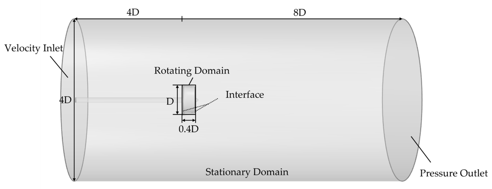
The Parasolid geometries generated in Siemens NX 2412 are imported into the commercial ANSYS Fluent 2024 R2 environment for mesh generation and CFD analysis; no custom CFD solver is used. Open-water CFD simulations are performed for the parameterized ducted propeller geometries. The domain comprises an inner rotating region and an outer stationary cylindrical region. The inlet is positioned 4D upstream, the outlet 8D downstream, and the far-field diameter is 4D. The rotating region encloses the propeller and its immediate flow field and has an axial length of approximately 0.4D. An interface transfers flow variables between the rotating and stationary regions, as illustrated in Figure 3.

A velocity-inlet condition is imposed at the inlet, with inflow velocity V_A determined by the advance ratio J. The outlet uses a pressure-outlet condition with a reference pressure of 0 Pa, and the far-field surface is treated as a slip wall. The propeller, duct, and hub surfaces are all specified as no-slip walls.

4.2.2. Solver Settings

All simulations were performed using ANSYS Fluent 2024 R2 in steady RANS mode. Propeller rotation was represented using a steady multiple-reference-frame (MRF) formulation implemented through the built-in Frame Motion option in ANSYS Fluent 2024 R2. The shear stress transport (SST) k-ω turbulence model was used to simulate viscous flow around the ducted propeller. Near-wall regions were resolved using 12 uniform-offset boundary-layer cells with a first-layer height of 0.01 mm and a growth rate of 1.15. The same boundary-layer settings were applied to the blade, duct, and hub wall regions, and wall y⁺ remained below 1 over the boundary-layer-resolved surfaces.

The propeller speed is fixed at n = 450 rpm, and different advance ratios J are produced by varying the inlet velocity V_A. Pressure-velocity coupling uses the SIMPLEC algorithm. For the adopted medium-resolution mesh, the minimum blade-tip clearance is 1 mm and is resolved by approximately 46 cell layers in the wall-normal gap direction, comprising approximately 12 blade-side boundary-layer cells, 22 core-volume cells, and 12 duct-side boundary-layer cells. A simulation is considered converged when residuals fall below 10⁻⁵ and the monitored thrust and torque become stable with further iterations. Water is modeled with density ρ = 998.2 kg/m³ and dynamic viscosity μ = 1.003 × 10⁻³ Pa s.

4.2.3. Grid-Convergence and Discretization-Uncertainty Assessment

Because the CFD database supplies both the sensitivity surrogates and the neural-network targets, numerical consistency is essential to the subsequent analysis. A three-level grid-refinement study was therefore performed for the standard Ka4-70/No. 19A benchmark configuration at two representative operating conditions, J = 0.3 and J = 0.6. The former corresponds to the lower bound of the investigated advance-ratio interval, whereas J = 0.6 represents the design operating condition. This two-condition assessment extends the previous single-condition mesh check and provides a quantitative evaluation of discretization uncertainty at both a low-advance-ratio condition and the design condition.

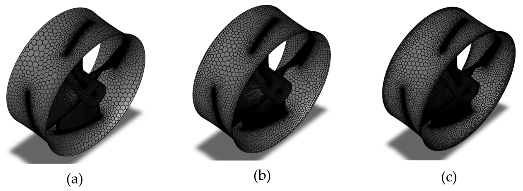
Unstructured meshes were locally refined near the blade leading edges, blade tips, and duct inner surface, where strong flow gradients are expected. The coarse, medium, and fine full-domain meshes contain 4,187,724, 8,204,688, and 13,612,796 cells, respectively. The three grid levels used in the discretization-uncertainty assessment are shown in Figure 4. The geometry, computational domain, physical models, boundary conditions, solver settings, and refinement-region locations were kept unchanged among the three grid levels, while the spatial resolution was progressively refined. For the same three-dimensional computational domain, the effective characteristic grid size is proportional to N_cell^−1/3, where N_cell is the total cell count. The resulting effective refinement ratios are r₂₁ = 1.184 between the fine and medium grids and r₃₂ = 1.251 between the medium and coarse grids.

For each hydrodynamic quantity S, the fine-, medium-, and coarse-grid solutions are denoted by S₁, S₂, and S₃, respectively. The successive solution changes are defined as ε₂₁ = S₂ − S₁ and ε₃₂ = S₃ − S₂, and the grid-convergence ratio is R_G = ε₂₁/ε₃₂. According to the ITTC CFD verification framework, 0 < R_G < 1 denotes monotonic convergence, whereas −1 < R_G < 0 denotes oscillatory convergence [26,27]. All six sequences obtained for K_T, 10K_Q and η at the two investigated advance ratios fall within the oscillatory-convergence regime. Consequently, a conventional Richardson extrapolation-based Grid Convergence Index (GCI), which relies on a monotonic asymptotic sequence, is not imposed on these data. Instead, the grid uncertainty for each oscillatory sequence is conservatively estimated as U_G = 1/2(S_max − S_min), following the ITTC treatment of oscillatory grid convergence [27]. For quantitative comparison, the relative grid uncertainty is normalized by the corresponding medium-grid solution as $U_{G,rel}=U_G/\left|S_2\right|\times 100\%$, because the medium grid is the resolution adopted for the subsequent CFD database. The medium-to-fine difference is calculated as $\left|S_1-S_2\right|/\left|S_1\right|\times 100\%$.

The convergence ratios in

Table 3. Three-grid convergence and discretization-uncertainty assessment at J = 0.3 and J = 0.6.

J	Quantity	Coarse	Medium	Fine	RG	Medium–Fine Difference (%)	Relative UG (%)
0.3	KT	0.37778	0.37669	0.37715	−0.424	0.12	0.14
0.3	10KQ	0.43063	0.42781	0.42873	−0.325	0.21	0.33
0.3	η	0.41887	0.42041	0.42003	−0.250	0.09	0.18
0.6	KT	0.2079	0.20348	0.20407	−0.133	0.29	1.09
0.6	10KQ	0.33519	0.33107	0.3319	−0.202	0.25	0.62
0.6	η	0.59229	0.58691	0.58713	−0.041	0.04	0.46

are negative but greater than −1 for all six hydrodynamic quantities, indicating oscillatory convergence rather than monotonic convergence or grid divergence. The relative grid-uncertainty estimates range from 0.14% to 1.09%. The largest value occurs for K_T at J = 0.6, whereas the remaining five quantities remain below 0.7%. These results indicate that the small non-monotonic changes observed among the three grids represent bounded oscillatory behavior rather than progressive divergence with grid refinement.

More importantly, for selection of the production mesh, refinement from 8,204,688 to 13,612,796 cells changes K_T, 10K_Q, and η by only 0.12%, 0.21%, and 0.09%, respectively, at J = 0.3, and by 0.29%, 0.25%, and 0.04% at J = 0.6. Thus, all medium-to-fine differences remain below 0.30%. Considering this limited sensitivity, together with the substantially higher computational cost of the fine grid, the approximately 8.2-million-cell mesh is retained as the accuracy–cost compromise for the subsequent parametric CFD database.

Because the present discretization-uncertainty assessment is conducted at J = 0.3 and J = 0.6, the quantified uncertainty estimates are associated with these two representative conditions and are not interpreted as a formal grid-convergence demonstration at every advance ratio over 0.3 ≤ J ≤ 0.7.

4.2.4. Benchmark Assessment of the Numerical Method

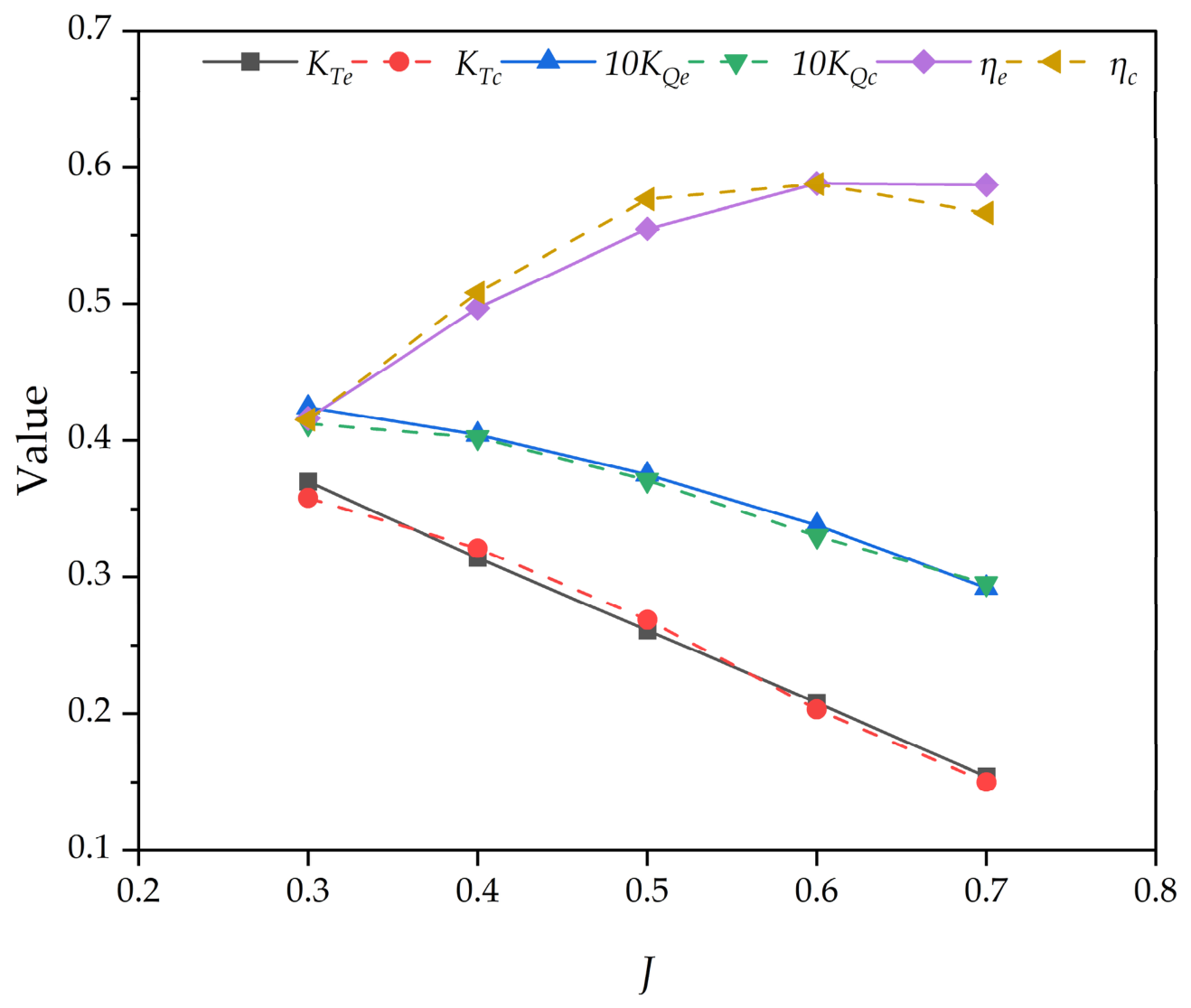
The approximately 8.2-million-cell medium-grid setup selected from the preceding grid-convergence assessment is further assessed by calculating the open-water characteristics of the standard Ka4-70/No. 19A configuration over multiple advance ratios. The validation propeller has a constant pitch ratio P/D = 1.0, and its radial geometry is defined in Table 1 from the standard Ka-series data of Sheng and Liu [22]. The computed K_T, 10K_Q, and η values are compared with the experimental reference data in Figure 5 [28,29].

This comparison provides external experimental support for the numerical setup used to generate the CFD database. It should be distinguished, however, from direct experimental validation of the modified parameterized designs: the 20 Ka4-70-derived geometries considered in the surrogate database are evaluated numerically in the present study, and no dedicated open-water experiment was conducted for an individually manufactured parameterized geometry.

4.3. Hydrodynamic Performance Results of the Parameterized Geometries

Using the benchmark-assessed numerical setup, open-water simulations are completed for all 20 parameterized geometries. Each geometry is evaluated at J = 0.3, 0.4, 0.5, 0.6, and 0.7, while the rotational speed remains n = 450 rpm. The recorded thrust and torque are converted into dimensionless hydrodynamic coefficients.

The total ducted propeller thrust is the sum of the propeller-blade thrust and the duct thrust. The corresponding thrust coefficients are defined as follows:

$$K_{TP}={\displaystyle \frac{T_P}{\rho n^2{D}^4}}$$

(26)

$$K_{TD}={\displaystyle \frac{T_D}{\rho n^2{D}^4}}$$

(27)

$$K_T=K_{TP}+K_{TD}$$

(28)

where T_P is the blade thrust, T_D is the duct thrust, and D is the propeller diameter used consistently in Equations (26)–(30). The torque coefficient and open-water efficiency are defined as

$$K_Q={\displaystyle \frac{Q}{\rho n^2{D}^5}}$$

(29)

$$\eta ={\displaystyle \frac{T{V}_A}{2\pi nQ}}$$

(30)

where Q is the torque, T the total ducted propeller thrust, V_A the inlet velocity, and n the rotational speed. These calculations yield 100 geometry-operating-condition observations from 20 independent geometries.

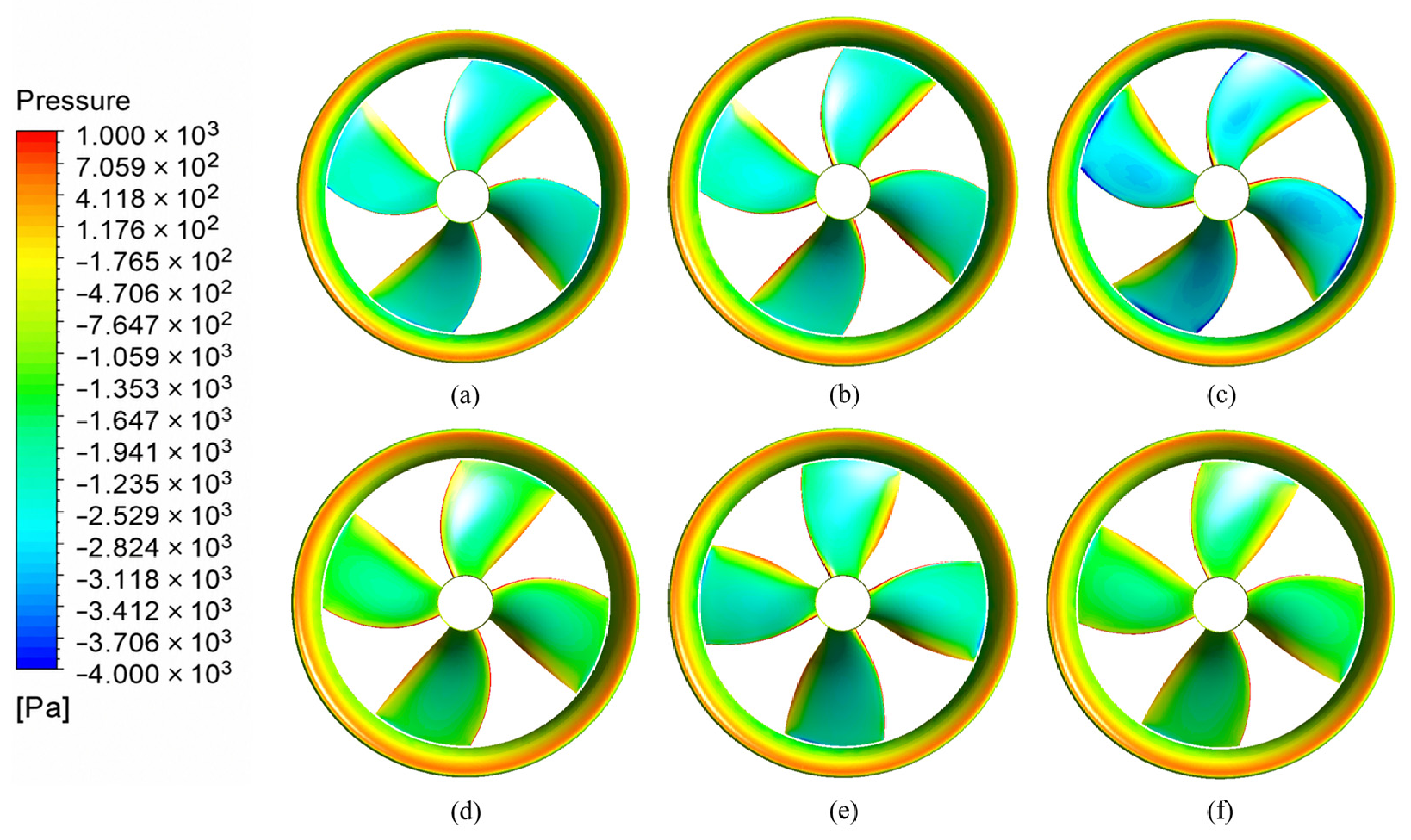
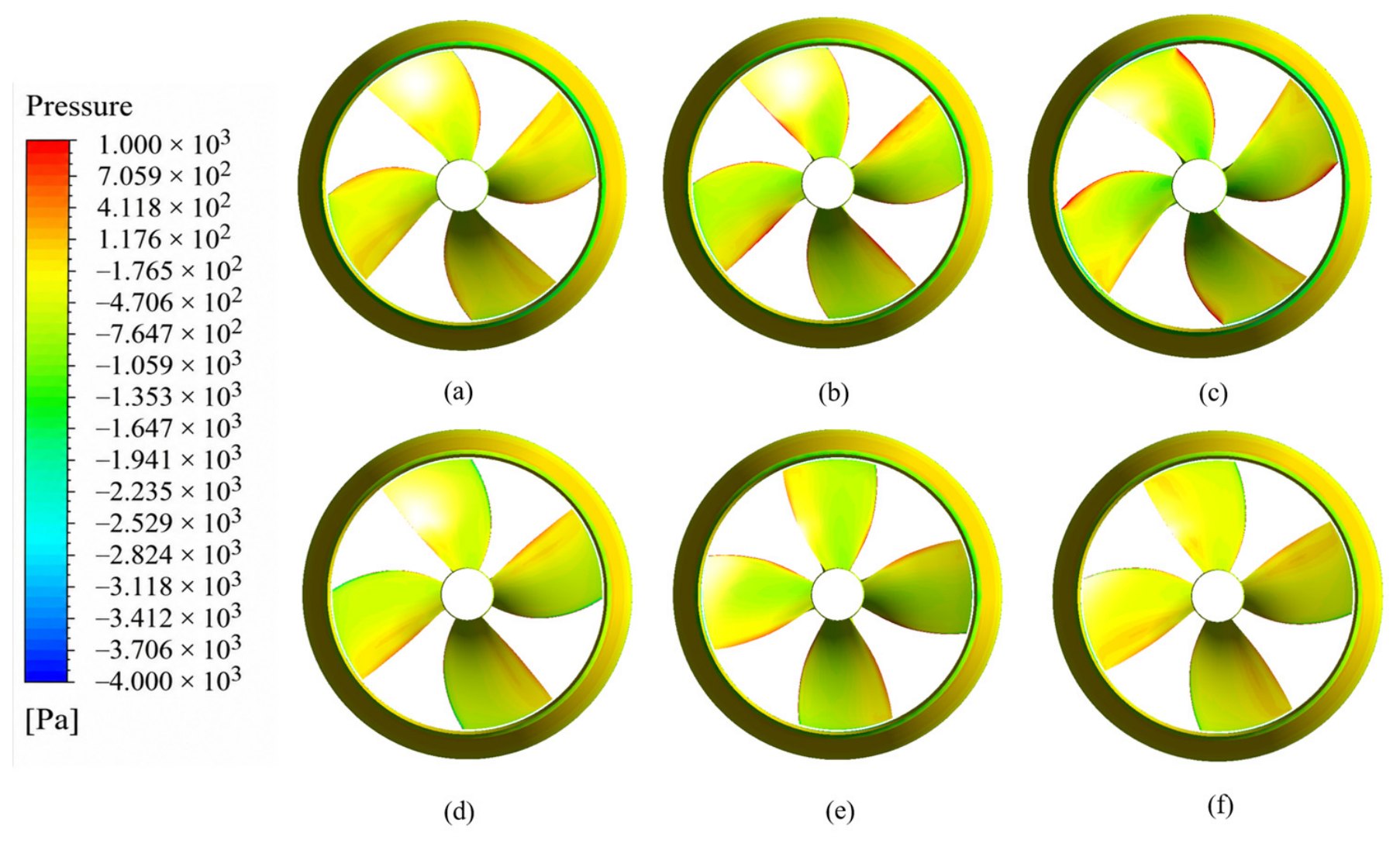
Samples 3, 8, 12, 13, 15, and 17 are selected for comparative flow-field visualization because they span contrasting combinations of pitch ratio, skew angle, and rake angle. The comparison is performed at J = 0.6.

Figure 6 and Figure 7 reveal clear differences in blade-surface pressure among the selected geometries. Sample 12 develops a more extensive low-pressure region on the suction side, whereas Samples 13 and 17 exhibit weaker suction-side negative pressure associated with their larger rake angles. On the pressure side, larger rake angles are also accompanied by more localized positive-pressure accumulation. These qualitative comparisons indicate pronounced effects of rake angle and pitch ratio on the surface-pressure field; the separate contributions of skew angle and thickness ratio are examined quantitatively through the conditional sensitivity analysis.

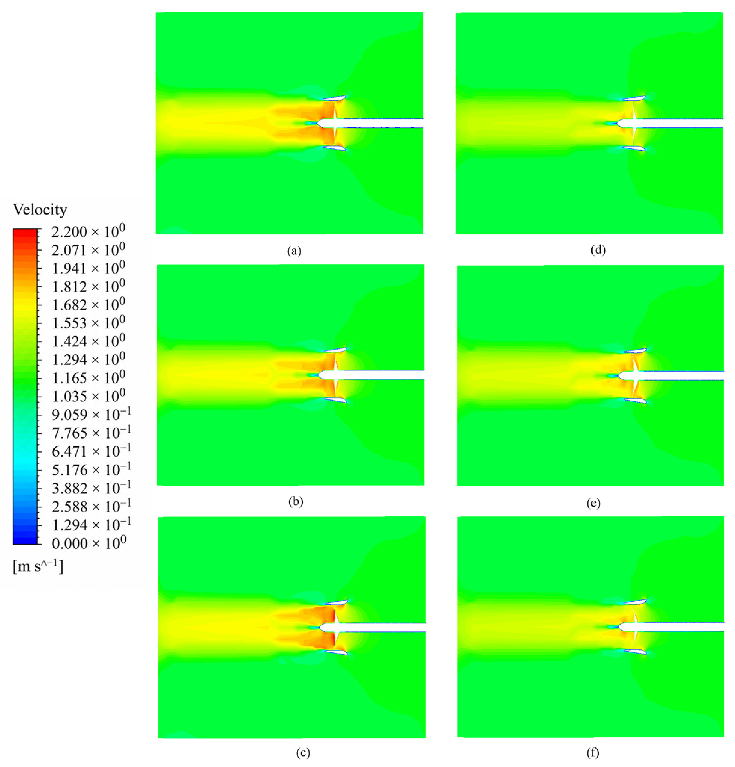
Figure 8 further shows geometry-dependent differences in the flow-acceleration region inside the duct and in the downstream wake. Smaller rake angles generally retain stronger axial acceleration, whereas larger rake angles may increase wake deflection and reduce axial kinetic energy retention. Sample 3 does not show a comparable reduction in velocity, suggesting that pitch ratio and other parameters modulate the rake effect. The flow fields, therefore, provide qualitative evidence of coupled geometric influences rather than isolated one-variable behavior.

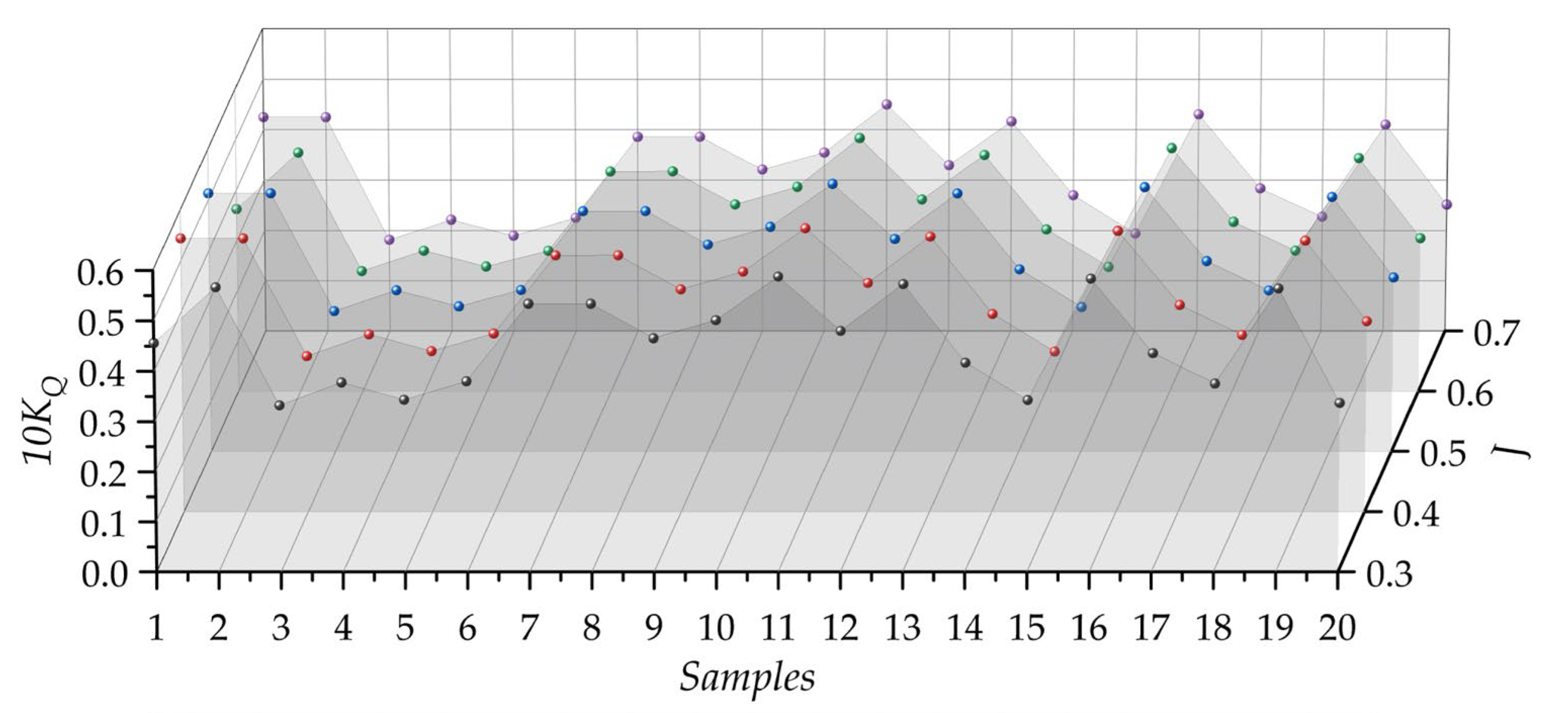
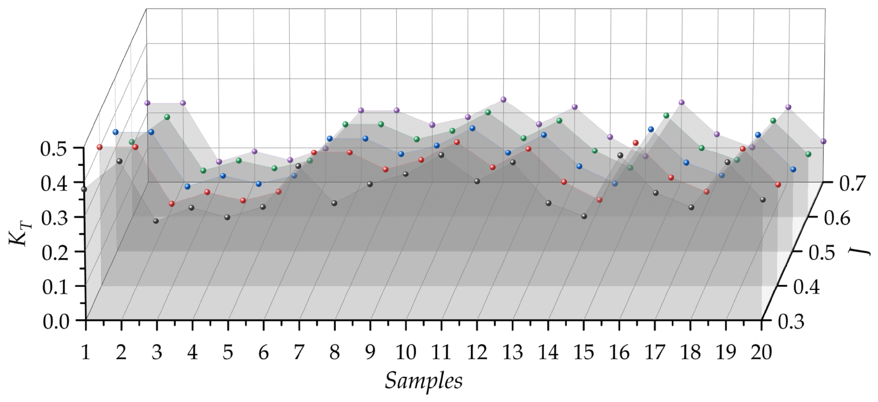
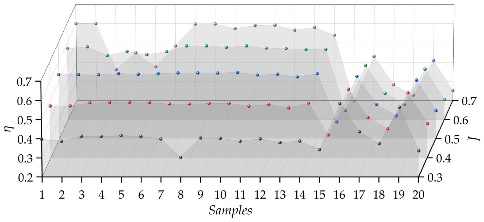
The K_T, 10K_Q, and eta values of all 20 geometries are summarized in Figure 9, Figure 10 and Figure 11 to compare their performance over the five advance ratios.

Figure 9, Figure 10 and Figure 11 show substantial nonlinear variation in K_T, 10K_Q, and eta across geometries and advance ratios. Higher thrust does not necessarily produce higher efficiency because torque demand and flow losses also govern energy conversion. The resulting multi-output, curve-level response supports the need for a nonlinear surrogate that represents operating progression and geometry-induced variation within a unified model.

4.4. Dataset Construction and Basis for Subsequent Modeling

The 20 parameterized geometries evaluated at five advance-ratio conditions produce 100 geometry-operating-condition observations. The i-th observation is denoted by the feature-response record d_i and is expressed as

$$d_i=\left\{J_{\mathrm{i}},(P/d{)}_i,{\theta }_{s,i},R_{k,i},(t/D{)}_i,K_{T,i},K_{Q,i}\right\}$$

(31)

where i is the observation index. The complete dataset is denoted by calligraphic D and is represented as

$$\mathcal{D}={\left\{d_i\right\}}_{i=1}^N,\hspace{1em}N=100.$$

(32)

where N = 100. Before training, the data are checked and standardized using statistics estimated exclusively from the relevant training subset. For conditional sensitivity estimation, the observations are reorganized into 20 complete geometry curves, each containing the five fixed J responses required for fitting and validating the curve surrogates in Section 5.

5. Sensitivity Analysis of Hydrodynamic Performance Parameters of the Ducted Propeller

5.1. CFD Data Grouping and Conditional Analysis Framework

The CFD database comprises 20 independent geometries sampled within P/D $\in$ [0.9, 1.2], θ_s $\in$ [0°, 35°], R_k $\in$ [0°, 12°], and t/D $\in$ [0.08, 0.14]. Every geometry is evaluated at J = 0.3, 0.4, 0.5, 0.6, and 0.7, and its five operating rows jointly define one complete performance curve. Conditional sensitivity estimation therefore groups the data by geometry and fixes J rather than treating it as another independently sampled uncertain input.

$$X=\left[J,P/D,{\theta }_s,R_k,t/D\right]$$

(33)

$$Y=\left[K_T,K_Q\right]$$

(34)

The conditional analysis measures geometry-induced variability in K_T and 10K_Q at a specified operating point. Within SIPR-BP, these estimates are not used as fixed physical coefficients; instead, they initialize output-specific soft priors for the four geometry gates, while J remains exclusively the coordinate of the ordered curve.

5.2. PLS Curve Surrogates and Conditional Sobol Estimation

Sobol indices are based on variance decomposition for mutually independent inputs [30]. At each fixed J, the four geometric variables are modeled as independent uniform variables over the Latin hypercube bounds. One two-component multi-output PLS regression maps normalized geometry to the five-node K_T curve, and a second maps geometry to the five-node 10K_Q curve [31]. During leave-one-geometry-out validation, the complete five-point curve of the held-out geometry is excluded from surrogate fitting.

$$Y=f\left(X_1,X_2,\cdots ,X_m\right)$$

(35)

The output variance is decomposed as

$$V(Y)={\displaystyle {\displaystyle \sum _{i=1}^m}{V}_i+}{\displaystyle \sum _{i<j}{V}_{ij}}+\cdots +V_{12\cdots m}$$

(36)

where V_i is the variance contribution associated with the independent effect of input X_i, and V_ij is the contribution associated with the interaction between X_i and X_j. The first-order and total-effect sensitivity indices are defined as

$$S_i={\displaystyle \frac{V_i}{V(Y)}}$$

(37)

$$S_{T_i}=1-{\displaystyle \frac{V_{~i}}{V(Y)}}$$

(38)

For each response at each fixed J, independently scrambled Sobol digital nets generate matrices A, B, and AB(i). S₁ is estimated using the Saltelli covariance estimator, and S_T is estimated using the Jansen estimator [32,33]. Full-data reporting uses 4096 base points and 16 independent scrambles; the 2.5th–97.5th percentiles therefore represent numerical integration variability only. More importantly, gate construction is fold-specific: every neural network outer fold refits the PLS models on its 18 training geometries and recomputes the indices using 2048 base points and four independent scrambles.

5.3. Leave-One-Geometry-Out Surrogate Validation

Table 4. Strict leave-one-geometry-out validation of the two-component PLS curve surrogates.

Criterion	MAPE (%)	RMSE	Q2	J	Output
Pass	4.00	0.0223	0.872	0.3	KT
Pass	3.73	0.0206	0.887	0.4	KT
Pass	4.32	0.0201	0.882	0.5	KT
Pass	2.24	0.0071	0.983	0.6	KT
Pass	7.90	0.0211	0.880	0.7	KT
Pass	3.37	0.0214	0.943	0.3	10KQ
Pass	4.28	0.0305	0.882	0.4	10KQ
Pass	4.64	0.0309	0.879	0.5	10KQ
Pass	2.29	0.0131	0.977	0.6	10KQ
Pass	6.09	0.0322	0.875	0.7	10KQ

reports strict leave-one-geometry-out predictive performance. For each held-out geometry, all five J rows are removed before fitting and are predicted jointly as one curve. Across the ten response nodes, predictive Q² ranges from 0.872 to 0.983, RMSE from 0.0071 to 0.0322, and MAPE from 2.24% to 7.90%. Every nodewise Q² exceeds the prespecified reporting threshold of 0.80, supporting the use of the low-complexity PLS models for fold-wise prior construction. Complete strict leave-one-geometry-out K_T(J) and 10K_Q(J) curves for all 20 geometries are provided in Supplementary Figures S1–S20.

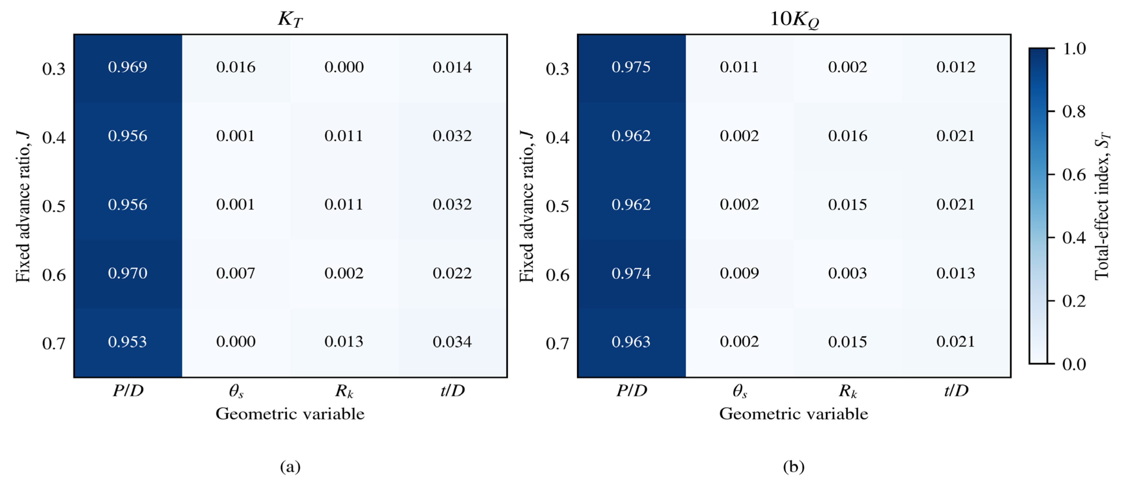
In Figure 12, each numerical label represents the conditional total-effect Sobol index S_T of the corresponding geometric variable at the specified fixed J, while the color intensity indicates its magnitude on the 0–1 scale. These indices quantify geometry-induced sensitivity within the adopted PLS surrogate and the sampled geometric bounds. They are used to construct fold-specific gate priors and should not be interpreted as the final trained neural network gate values.

These diagnostics indicate that the PLS curve models provide stable, low-complexity interpolation within the sampled geometric bounds. Accordingly, the conditional indices are reported only for the defined uniform ranges, and every gate prior is reconstructed whenever the outer training set changes. The indices are therefore used as fold-specific guidance rather than as universal physical attribution coefficients or as final learned gate weights.

5.4. Conditional Geometric Sensitivity at Fixed Advance Ratio

Figure 12 shows the conditional total-effect indices at the five fixed J levels. For K_T, the P/D index ranges from 0.953 to 0.970; for 10K_Q, it ranges from 0.962 to 0.975. Thus, P/D is identified as the dominant contributor to geometry-induced variance throughout the investigated operating range.

The conditional effects of the remaining variables are substantially smaller. Depending on J, θ_s, R_k, and t/D contribute at most 0.016, 0.013, and 0.034 for K_T and at most 0.011, 0.016, and 0.021 for 10K_Q. Because the adopted PLS models are linear in geometry, their first-order and total-effect estimates are nearly identical. The analysis is therefore interpreted as a stable main-effect ranking within the sampled bounds, which is sufficient for constructing a weak gate prior but not for resolving higher-order nonlinear interactions.

5.5. Fold-Specific Gate Priors and Interpretation

For each output, the conditional S_T values are aggregated across the five fixed J levels using the corresponding surrogate-output variances and then normalized over the four geometry variables. The resulting full-data priors assign proportions of 0.9605 and 0.9670 to P/D for K_T and 10K_Q, respectively.

The ten outer-fold priors remain stable despite changes in the training geometries: the P/D proportion ranges from approximately 0.947 to 0.989 for K_T and from 0.954 to 0.991 for 10K_Q.

Table 5. Full-data geometry-gate priors and their variation across the ten outer training folds.

Variable	Output	Full-Data Prior	Fold Mean	Fold Minimum	Fold Maximum
P/D	KT	0.9605	0.9597	0.9465	0.9887
θs	KT	0.0048	0.0059	0.0016	0.0115
Rk	KT	0.0077	0.0068	0.0002	0.0111
t/D	KT	0.0270	0.0276	0.0094	0.0397
P/D	10KQ	0.9670	0.9663	0.9539	0.9905
θs	10KQ	0.0051	0.0062	0.0012	0.0152
Rk	10KQ	0.0103	0.0094	0.0002	0.0177
t/D	10KQ	0.0176	0.0180	0.0081	0.0295

reports the corresponding fold-wise ranges for all four variables.

During SIPR-BP training, J remains an ungated coordinate that locates the operating point on the ordered curve. Only the four geometry descriptors receive output-specific positive gates, initialized from the corresponding fold-specific prior. Because the prior enters through a weak penalty, the gate ranking is physically guided but remains trainable and prediction-adaptive.

This separation gives operating conditions and geometry distinct modeling roles: J parameterizes progression along a performance curve, whereas the conditional indices characterize geometry-induced variability at a fixed operating point. The resulting prior is therefore more targeted than applying a single global importance vector to all five inputs and preserves the ordered dependence on J.

6. Geometry-Grouped Hydrodynamic Performance Prediction and Validation

6.1. Balanced Geometry-Grouped Validation and Implementation Settings

A fixed balanced geometry-group holdout protocol is used to assess predictions for previously unseen geometries. The ten test pairs are (11,10), (8,16), (15,2), (9,5), (1,12), (6,17), (14,7), (20,13), (4,3), and (18,19). In each round, the complete five-point curves of both test geometries are withheld, and the remaining 18 geometries are used for model development. Every geometry is therefore evaluated exactly once as an unseen object. Crucially, no operating row from a held-out geometry enters standardization, PLS fitting, conditional Sobol estimation, reliability weighting, or neural network training.

All candidate models use identical outer partitions and are evaluated on the complete unweighted test curves. The PLS curve surrogate is refitted directly on the 18 outer-training geometries in each round and evaluated on the same two held-out geometries as SIPR-BP. For SVR, GPR, and Extra Trees, hyperparameters are selected by geometry-grouped cross-validation conducted solely within the 18 training geometries of each outer round. All five operating conditions of a geometry remain in the same subset throughout model selection. Each benchmark is then refitted on the full set of 18 training geometries and evaluated on the two held-out geometries [34,35,36].

Table 6. Implementation settings for SIPR-BP.

Item	Setting
Validation protocol	10 balanced geometry-grouped holdout rounds; 18 training geometries and 2 test geometries per round
Inputs and outputs	Inputs: J, P/D, θs, Rk, and t/D; outputs: KT and 10KQ
Curve branches	Independent 4-24-16-5 branches for KT and 10KQ with SiLU activation
Monotone nodes	Five ordered nodes over J = 0.3–0.7 with piecewise-linear interpolation
Optimization	AdamW, cosine-annealing learning rate schedule, and gradient-clipping threshold of 10
Main training parameters	400 epochs; initial learning rate 2.5 × 10−3; weight decay 2 × 10−4
Regularization weights	λg = 10−2; λc = 10−5
Sensitivity-gate prior	Two-component PLS curve surrogate; conditional ST at five fixed J levels; 2048 base points and four independent scrambles per outer fold
Reliability weights	0.05–1.00; estimated exclusively from the current training geometries
Ensemble size	Three independently initialized members; their mean is the final prediction
Primary metrics	Geometry-balanced mean MAPE and geometry-averaged R2; RMSE and MAE are supplementary

summarizes the SIPR-BP implementation. Within every outer fold, the input and output scalers, two-component PLS curve surrogates, conditional Sobol gate priors, and reliability weights are all reconstructed from the current training geometries. The four geometry-gate priors are therefore fold-specific, whereas J remains the ungated coordinate used for ordered-curve interpolation.

The protocol distinguishes true geometry-level prediction from interpolation among operating points of a geometry already seen during training. By blocking information transfer through preprocessing, sensitivity estimation, reliability construction, and benchmark selection, it creates a leakage-resistant basis for the subsequent ablation, benchmark, statistical, and physical consistency analyses.

6.2. Ablation Study

The ablation study quantifies the incremental and coordinated contributions of fold-specific conditional sensitivity gating, structural monotonicity, reliability-based soft weighting, and ensemble averaging.

Table 7. Definitions of the ablation models.

Model	Components
A0 BP-Raw	Five original physical variables with a conventional two-output BP architecture
A1 SI-BP	A0 plus output-specific, fold-specific conditional Sobol gates computed only from the outer-training geometries
A2 SIPR-BP-Mono	A1 plus structurally monotonic performance curves along J
A3 SIPR-BP-Reliability	A2 plus continuous reliability weights estimated only within the training fold
A4 SIPR-BP	A3 plus a three-member deep ensemble

defines the five configurations, all of which use the same geometry-grouped training and test partitions.

Table 8. Geometry-balanced ablation results for the 20 unseen geometries.

Model	MAPE (%)	RMSE	MAE	Geometry-Averaged R2	Pooled Out-of-Group R2
A0 BP-Raw	4.51	0.0158	0.0135	0.855	0.944
A1 SI-BP	3.24	0.0127	0.0103	0.869	0.949
A2 SIPR-BP-Mono	3.10	0.0124	0.0104	0.866	0.948
A3 SIPR-BP-Reliability	2.83	0.0116	0.00963	0.869	0.949
SIPR-BP	2.65	0.0112	0.00911	0.875	0.951

reports geometry-balanced performance over all 20 held-out geometries. MAPE and geometry-averaged R² are used as the primary ranking criteria, while RMSE, MAE, and pooled out-of-group R² provide complementary measures of absolute error and global response reconstruction.

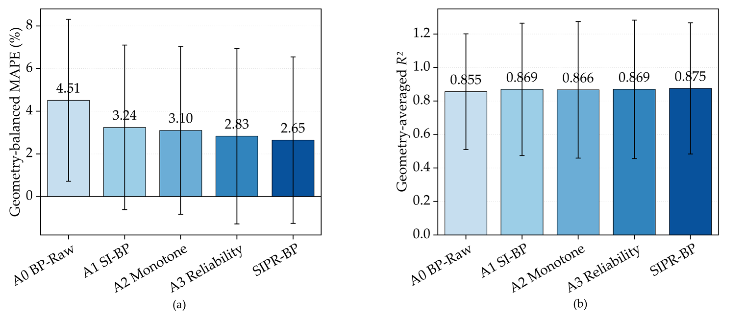
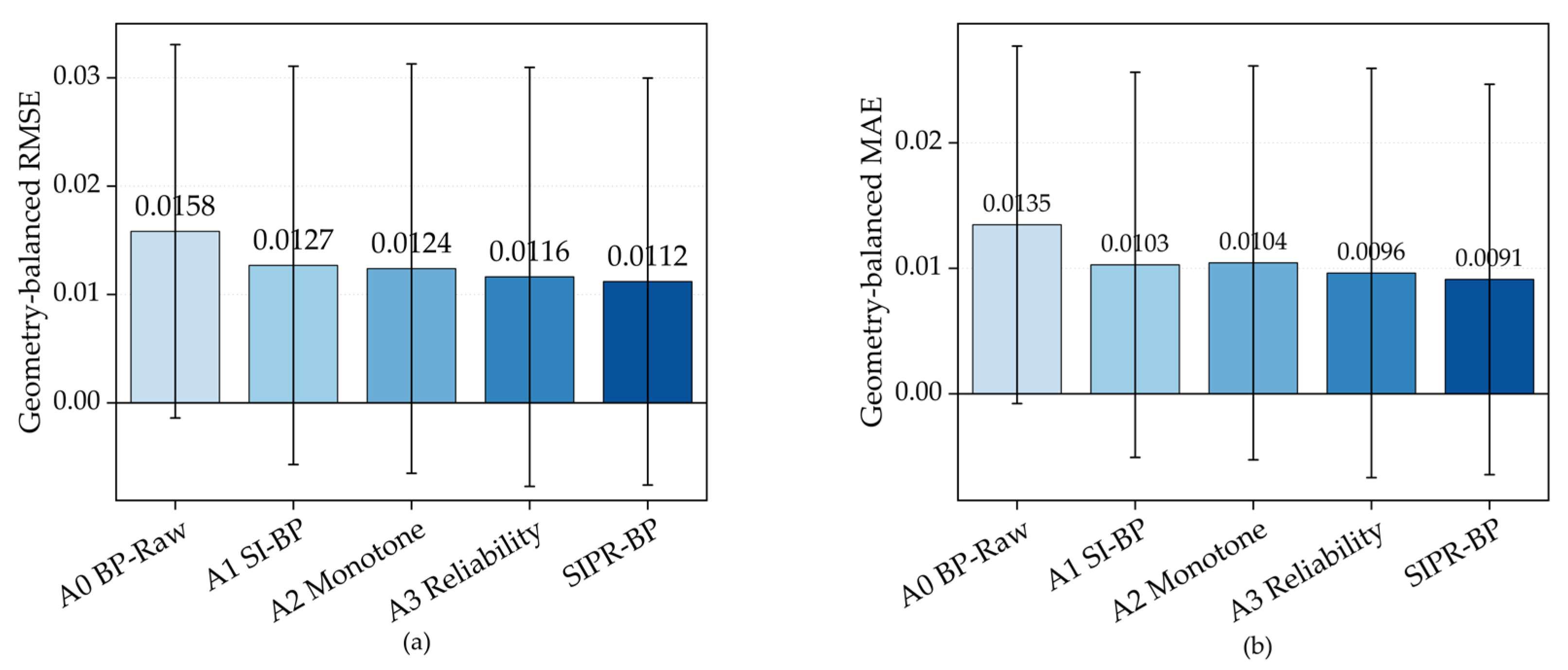
Figure 13 and Figure 14 visualize the ablation results. Each bar represents the mean geometry-level metric, and each error bar indicates the corresponding standard deviation across the 20 held-out geometries. Figure 13 presents the two primary criteria, whereas Figure 14 presents the complementary absolute-error measures.

SIPR-BP achieves the best overall geometry-balanced performance, with a mean MAPE of 2.65%, an RMSE of 0.0112, and an MAE of 0.00911. Its geometry-averaged R² is 0.875, and its pooled out-of-group R² reaches 0.951. The concurrent improvement in geometry-level and pooled metrics indicates that the framework reconstructs both individual unseen curves and the global hydrodynamic response trend.

The ablation results indicate complementary rather than uniformly monotonic contributions of the individual modules. Sensitivity gating produces the largest initial reduction in geometry-balanced error. Adding the ordered-node structure further reduces MAPE from 3.24% to 3.10% and, more importantly, introduces an exact non-increasing curve constraint. However, geometry-averaged R² decreases slightly from 0.869 to 0.866, and pooled R² from 0.949 to 0.948. Reliability weighting subsequently improves the balance of the predictive metrics, while the three-member ensemble provides the lowest final MAPE, RMSE, and MAE. Relative to A3, the final ensemble wins on 15 of 20 geometries and yields a one-sided p = 0.0379.

6.3. Comparison with Other Surrogate Models

To determine whether the integrated design provides an advantage beyond both its own low-complexity prior model and conventional data-driven surrogates, SIPR-BP is compared with the two-component PLS curve surrogate, Extra Trees, Gaussian process regression (GPR), and support vector regression (SVR). For a strictly matched comparison, PLS is evaluated using exactly the same ten outer partitions as SIPR-BP, with 18 training geometries and two unseen test geometries per round. The remaining benchmarks undergo training-only geometry-grouped hyperparameter selection and are evaluated on the same unseen geometries.

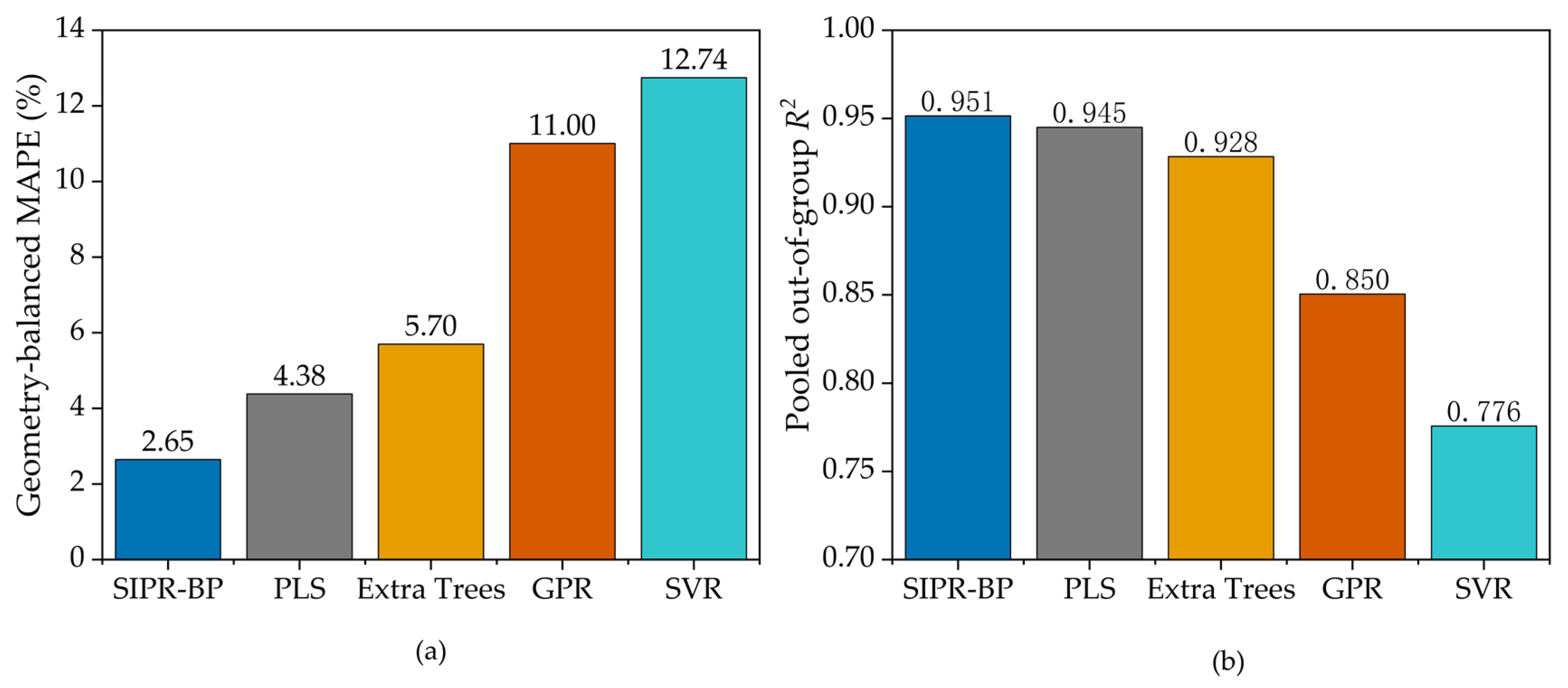
Figure 15 directly compares geometry-balanced mean MAPE and pooled out-of-group R² for SIPR-BP and the four baseline models. The figure reports the aggregate values listed in

Table 9. Comparison with representative data-driven surrogate models.

Model	MAPE (%)	RMSE	MAE	Geometry-Averaged R2	Pooled Out-of-Group R2
SIPR-BP	2.65	0.0112	0.00911	0.875	0.951
PLS curve surrogate	4.38	0.0165	0.0145	0.848	0.945
Extra Trees	5.70	0.0194	0.0170	0.809	0.928
GPR	11.00	0.0322	0.0293	0.569	0.850
SVR	12.74	0.0396	0.0347	0.365	0.776

.

SIPR-BP reduces geometry-balanced MAPE by approximately 39.6%, 53.6%, 76.0%, and 79.2% relative to PLS, Extra Trees, GPR, and SVR, respectively. Its pooled out-of-group R² is 0.951, compared with 0.945, 0.928, 0.850, and 0.776 for the four baselines. The matched-fold PLS result confirms that the low-complexity curve surrogate is itself competitive; the additional benefit of SIPR-BP is expressed in lower geometry-level error, together with the prescribed monotonic curve structure and training-only reliability weighting.

6.4. Paired Statistical Analysis

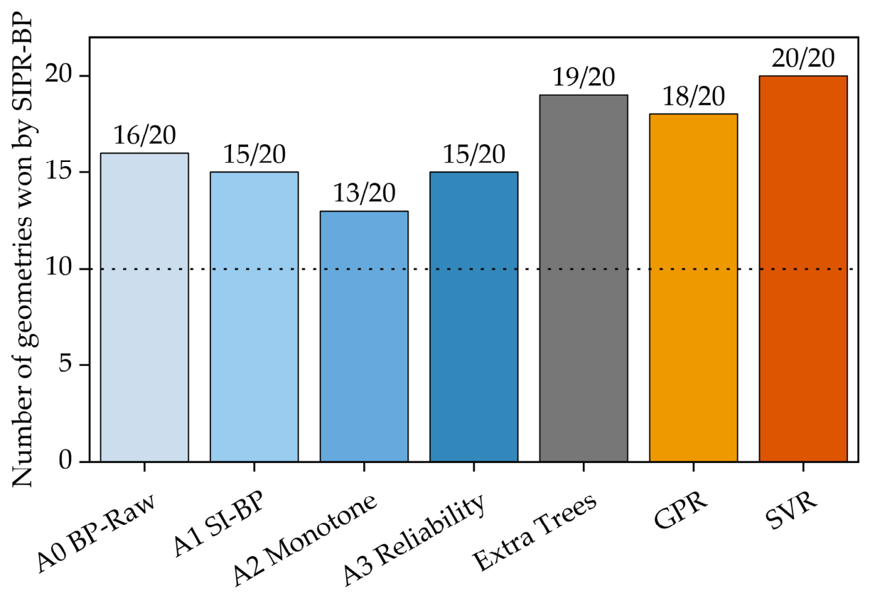
Aggregate means do not show whether an improvement is repeated across individual geometries. A paired analysis is therefore conducted on the geometry-level MAPE values obtained from the same 20 held-out geometries. The matched-fold PLS curve surrogate is retained as an aggregate low-complexity baseline in Table 9, whereas the paired significance analysis in

Table 10. Geometry-level paired comparisons with SIPR-BP as the reference model.

Comparator	SIPR-BP Wins	Mean MAPE Reduction (%)	One-Sided p-Value
A0 BP-Raw	16/20	39.20	4.25 × 10−4
A1 SI-BP	15/20	13.63	0.00859
A2 SIPR-BP-Mono	13/20	13.27	0.00681
A3 SIPR-BP-Reliability	15/20	5.85	0.0379
Extra Trees	19/20	48.95	2.86 × 10−6
GPR	18/20	62.62	2.38 × 10−5
SVR	20/20	72.92	9.54 × 10−7

follows the pre-specified geometry-level comparisons available for the ablation variants and the three conventional benchmark models. For these seven comparators, Table 10 reports the SIPR-BP win count, mean percentage reduction in MAPE, and the one-sided Wilcoxon signed-rank p-value for the hypothesis that the comparator has the larger error.

Figure 16 summarizes the geometry-level win counts. Values above 10 indicate that SIPR-BP achieves a lower MAPE than the comparator for a majority of the unseen geometries.

SIPR-BP yields lower geometry-level errors than A0, A1, A2, and A3, with one-sided p-values of 4.25 × 10⁻⁴, 0.00859, 0.00681, and 0.0379, respectively. The comparisons with Extra Trees, GPR, and SVR also favor SIPR-BP, with p-values of 2.86 × 10⁻⁶, 2.38 × 10⁻⁵, and 9.54 × 10⁻⁷, respectively. Together with the win counts and effect magnitudes, these tests provide geometry-level evidence that the improvement is not driven by only a small subset of designs.

6.5. Physical-Consistency Audit

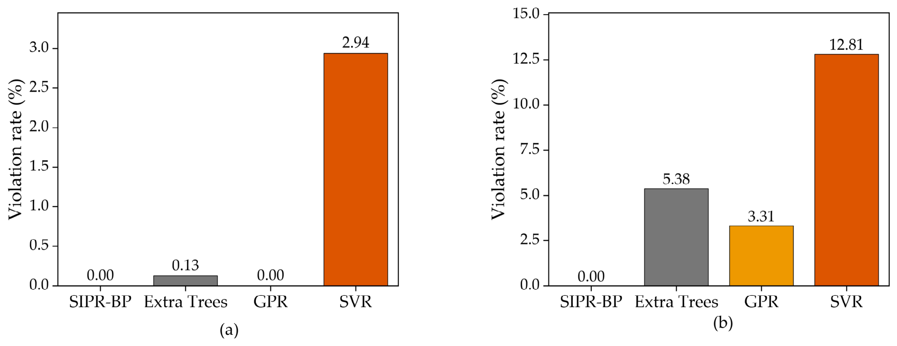
Accuracy evaluation is complemented by a physical-consistency audit on a dense advance-ratio grid. For every held-out geometry, each trained model is evaluated at 81 equally spaced J values from 0.3 to 0.7. Positive adjacent increments are counted as violations of the expected non-increasing K_T–J or 10K_Q–J relationship, and all dense-grid outputs are checked for non-positive predictions. For SIPR-BP, zero monotonicity violations are an architectural consequence of the ordered-node representation; the dense-grid evaluation, therefore, serves as an implementation check rather than as independent evidence that monotonicity was learned from the data. For the unconstrained benchmarks, the same audit remains an empirical diagnostic.

Table 11. Physical-consistency audit on the dense J grid.

Model	KT Violation Rate	10KQ Violation Rate	Negative-Prediction Rate
SIPR-BP	0.000%	0.000%	0.000%
Extra Trees	0.125%	5.375%	0.000%
GPR	0.000%	3.312%	0.000%
SVR	2.938%	12.812%	0.000%

aggregates the results over all outer rounds.

Figure 17 separates the K_T and 10K_Q monotonicity violation rates. For SIPR-BP, the zero rate is guaranteed by construction rather than obtained through post-processing or inferred empirically.

SIPR-BP produces neither monotonicity violations nor negative predictions over the dense audit grid, as expected from the ordered-node construction. The 10K_Q violation rates of Extra Trees, GPR, and SVR are 5.375%, 3.312%, and 12.812%, respectively. Extra Trees and SVR also show K_T violation rates of 0.125% and 2.938%. Thus, Table 11 should be interpreted primarily as an empirical physical-consistency diagnostic for the unconstrained benchmarks and as an implementation verification for SIPR-BP.

6.6. Out-of-Group Prediction and Ensemble Stability

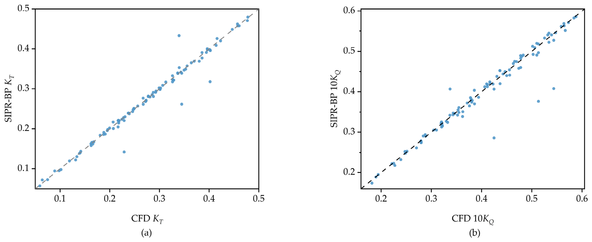
The ten outer rounds generate predictions at all five operating conditions for every geometry, yielding 100 strictly out-of-group observations derived from 20 independently held-out geometries. Figure 18 compares the pooled CFD values with the final three-member ensemble predictions for K_T and 10K_Q; the dashed diagonal denotes ideal agreement.

The pooled out-of-group R² values are 0.968 for K_T and 0.935 for 10K_Q. Predictions remain close to the ideal-agreement line over the response range, showing that SIPR-BP reconstructs variation associated with both geometry and operating conditions rather than merely fitting one dimension of the dataset.

In every outer round, the reported prediction is the arithmetic mean of three independently initialized networks trained with the same geometry-grouped data, fold-specific sensitivity priors, and reliability weights. This coordinated aggregation gives the lowest MAPE, RMSE, and MAE and improves geometry-level MAPE relative to the single reliability-weighted member A3 (p = 0.0379).

7. Discussion and Conclusions

This study establishes SIPR-BP as an integrated, geometry-aware surrogate for the performance of Ka4-70-derived parameterized ducted propellers. Its central methodological advance is the coupling of fold-reconstructed conditional sensitivity priors with structure-preserving neural curves. The operating coordinate J parameterizes a five-node ordered performance curve, whereas P/D, θ_s, R_k, and t/D are processed through output-specific trainable gates. In every outer fold, the gate priors are reconstructed from two-component PLS curve surrogates at fixed J using only the 18 training geometries. Training-only physics-consistency reliability weights, a reliability-weighted Smooth L1 objective, and a three-member ensemble complete the framework.

Under ten-round balanced geometry-group holdout validation, SIPR-BP achieves a geometry-balanced mean MAPE of 2.65%, RMSE of 0.0112, MAE of 0.00911, geometry-averaged R² of 0.875, and pooled out-of-group R² of 0.951. The newly included matched-fold PLS baseline achieves a MAPE of 4.38%, showing that the low-complexity curve surrogate itself is already competitive. SIPR-BP, nevertheless, reduces geometry-balanced MAPE by approximately 39.6% relative to PLS and by 53.6–79.2% relative to Extra Trees, GPR, and SVR, while additionally providing structurally guaranteed non-increasing performance curves and training-only reliability weighting.

The component analysis indicates complementary rather than strictly cumulative contributions. Sensitivity gating provides the largest initial error reduction, ordered nodes impose the prescribed response structure while not improving every R² metric in isolation, reliability weighting reduces the influence of locally trend-inconsistent training observations, and ensemble averaging gives the lowest final error. The zero dense-grid monotonicity violation rate of SIPR-BP is therefore interpreted as a consequence of the architecture rather than an independent empirical finding.

The conclusions are restricted to the 20 Ka4-70-derived geometries, the five investigated advance ratios, and the prescribed four-dimensional parameter bounds. The linear PLS surrogates intentionally provide a stable low-complexity main-effect ranking for prior construction and do not resolve nonlinear geometric interactions. Dedicated fabrication and open-water testing of selected newly generated parameterized ducted propeller geometries will be required before extrapolating the conclusions beyond the sampled domain. Future work will also expand the CFD design space, examine nonlinear sensitivity surrogates under nested geometry-group validation, propagate surrogate uncertainty into the gate priors, and extend the structure-preserving framework to additional hydrodynamic outputs.

References

1. Jin, Z.; Wang, P.; Dong, H.; An, X.; Xia, H. Numerical prediction of ducted propeller performance based on a BEM–RANS coupling method. Ocean Eng. 2023, 271, 113761. [Google Scholar] [CrossRef] [Scilit]
2. Li, Z.; Cao, X.; Qin, H.; Yin, C.; Xu, S. Structural optimization and experimental measurement of ducted propellers. Ocean Eng. 2026, 356, 125345. [Google Scholar] [CrossRef] [Scilit]
3. Zhang, Q.; Jaiman, R.K.; Ma, P.; Liu, J. Investigation on the performance of a ducted propeller in oblique flow. J. Offshore Mech. Arct. Eng. 2020, 142, 011801. [Google Scholar] [CrossRef] [Scilit]
4. Prakash, N.; Muthuvel, A.; Roychowdhury, D.G. Numerical simulation of a three-bladed marine propeller in steady and unsteady state. Appl. Mech. Mater. 2014, 592–594, 1136–1141. [Google Scholar] [CrossRef] [Scilit]
5. Saettone, S.; Taskar, B.; Regener, P.B.; Steen, S.; Andersen, P. A comparison between fully-unsteady and quasi-steady approach for the prediction of the propeller performance in waves. Appl. Ocean Res. 2020, 99, 102011. [Google Scholar] [CrossRef] [Scilit]
6. Ng’aru, J.M.; Park, S. CFD simulations of the effect of equalizing duct configurations on cavitating flow around a propeller. J. Mar. Sci. Eng. 2022, 10, 1865. [Google Scholar] [CrossRef] [Scilit]
7. Li, L.; Zhou, B.; Liu, D.; Wang, C. Numerical analysis of influence of the hull couple motion on the propeller exciting force characteristics. J. Mar. Sci. Eng. 2019, 7, 330. [Google Scholar] [CrossRef] [Scilit]
8. Zondervan, G.J.; Hoekstra, M.; Holtrop, J. Flow analysis, design and testing of ducted propellers. In Proceedings of the SNAME 11th Propeller and Shafting Symposium, Williamsburg, VA, USA, 1 September 2006. [Google Scholar] [CrossRef] [Scilit]
9. Valčić, M.; Dejhalla, R. Neural network prediction of open water characteristics of ducted propeller. Pomor. Zb. 2015, 49–50, 101–115. [Google Scholar] [CrossRef] [Scilit][Green Version]
10. Shora, M.M.; Ghassemi, H.; Nowruzi, H. Using computational fluid dynamic and artificial neural networks to predict the performance and cavitation volume of a propeller under different geometrical and physical characteristics. J. Mar. Eng. Technol. 2018, 17, 59–84. [Google Scholar] [CrossRef] [Scilit]
11. Dong, H.; Wang, J.; Wang, W.; Shen, J. Data-driven multi-task global optimization with two-stage knowledge transfer for blended-wing-body underwater gliders design. Appl. Soft Comput. 2026, 194, 114867. [Google Scholar] [CrossRef] [Scilit]
12. Neocleous, C.C.; Schizas, C.N. Artificial neural networks in marine propeller design. In Proceedings of the ICNN’95—International Conference on Neural Networks, Perth, WA, Australia, 27 November–1 December 1995; Volume 2, pp. 1098–1102. [Google Scholar] [CrossRef] [Scilit]
13. Neocleous, C.C.; Schizas, C.N. Marine propeller design using artificial neural networks. In Proceedings of the IJCNN’99—International Joint Conference on Neural Networks, Washington, DC, USA, 10–16 July 1999; Volume 6, pp. 3958–3961. [Google Scholar] [CrossRef] [Scilit]
14. Pan, Z.; Sun, X.L.; Zhang, Y.; Li, X.B.; Zhu, X.K.; Yang, L.C. Study on marine propeller design using artificial neural networks and multivariate analysis. In Proceedings of the 2023 IEEE 11th International Conference on Computer Science and Network Technology (ICCSNT), Dalian, China, 21–22 October 2023; pp. 169–180. [Google Scholar] [CrossRef] [Scilit]
15. Li, L.; Chen, Y.; Huang, L.; Hai, Q.; Tang, D.; Wang, C. Improvement of propeller hydrodynamic prediction model based on multitask ANN and its application in optimization design. J. Mar. Sci. Eng. 2025, 13, 183. [Google Scholar] [CrossRef] [Scilit]
16. Tadros, M.; Shi, W.; Xu, Y.; Song, Y. A unified cross-series marine propeller design method based on machine learning. Ocean Eng. 2024, 314, 119691. [Google Scholar] [CrossRef] [Scilit]
17. Dang, Z.; Wu, M.; He, X.; Huang, Z.; Ying, Z.; Chen, Z.; Zheng, C. Aquatic–aerial propeller optimization based on a multi-fidelity neural network and transfer learning. Phys. Fluids 2025, 37, 107121. [Google Scholar] [CrossRef] [Scilit]
18. Li, C.; Cao, Y.; Xu, H.; Jiang, T.; Liu, C. Energy-saving optimization design of propeller boss cap fin based on BP neural network coupled with northern goshawk optimization algorithm. Int. J. Energy Res. 2024, 2024, 8424160. [Google Scholar] [CrossRef] [Scilit]
19. Zhang, S.; Liu, G.; Cheng, C. Application of modified BP neural network in identification of unmanned surface vehicle dynamics. J. Mar. Sci. Eng. 2024, 12, 297. [Google Scholar] [CrossRef] [Scilit]
20. Zhai, X.Y.; Lu, J.G. Prediction of propeller open-water performance based on neural network. J. Nanjing Tech Univ. (Nat. Sci. Ed.) 2022, 44, 291–297. [Google Scholar] [CrossRef]
21. Huang, X.; Chen, Y.; Zhan, W.; Lin, J.; Zhang, Y. Motion control of robotic fish based on BP neural network–fuzzy fusion optimization algorithm. IEEJ Trans. Electr. Electron. Eng. 2026, 21, 1508–1520. [Google Scholar] [CrossRef] [Scilit]
22. Sheng, Z.; Liu, Y. Ship Principles, Volume II; Shanghai Jiao Tong University Press: Shanghai, China, 2011; p. 177. (In Chinese) [Google Scholar]
23. Sill, J. Monotonic networks. In Advances in Neural Information Processing Systems 10; MIT Press: Cambridge, MA, USA, 1998; pp. 661–667. [Google Scholar]
24. Ren, M.; Zeng, W.; Yang, B.; Urtasun, R. Learning to reweight examples for robust deep learning. In Proceedings of the 35th International Conference on Machine Learning, Stockholm, Sweden, 10–15 July 2018; Volume 80, pp. 4334–4343. [Google Scholar]
25. Lakshminarayanan, B.; Pritzel, A.; Blundell, C. Simple and scalable predictive uncertainty estimation using deep ensembles. In Advances in Neural Information Processing Systems 30; Curran Associates Inc.: Red Hook, NY, USA, 2017; pp. 6402–6413. [Google Scholar]
26. International Towing Tank Conference (ITTC). Uncertainty Analysis in CFD Verification and Validation Methodology and Procedures; Recommended Procedures and Guidelines 7.5-03-01-01, Revision 05; ITTC: Zürich, Switzerland, 2024. [Google Scholar]
27. International Towing Tank Conference (ITTC). Validation and Verification of RANS Solutions in the Prediction of Manoeuvring Capabilities; Recommended Procedures and Guidelines 7.5-03-04-02, Revision 03; ITTC: Zürich, Switzerland, 2024. [Google Scholar]
28. Oosterveld, M.W.C. Wake Adapted Ducted Propellers; NSMB Publication No. 345; NSMB: Wageningen, The Netherlands, 1970. [Google Scholar]
29. Oosterveld, M.W.C. Ducted propeller characteristics. In Proceedings of the Symposium on Ducted Propellers, Teddington, UK, 30 May–1 June 1973; pp. 35–69. [Google Scholar]
30. Sobol’, I.M. Global sensitivity indices for nonlinear mathematical models and their Monte Carlo estimates. Math. Comput. Simul. 2001, 55, 271–280. [Google Scholar] [CrossRef] [Scilit]
31. Geladi, P.; Kowalski, B.R. Partial least-squares regression: A tutorial. Anal. Chim. Acta 1986, 185, 1–17. [Google Scholar] [CrossRef] [Scilit]
32. Saltelli, A.; Annoni, P.; Azzini, I.; Campolongo, F.; Ratto, M.; Tarantola, S. Variance-based sensitivity analysis of model output: Design and estimator for the total sensitivity index. Comput. Phys. Commun. 2010, 181, 259–270. [Google Scholar] [CrossRef] [Scilit]
33. Jansen, M.J.W. Analysis of variance designs for model output. Comput. Phys. Commun. 1999, 117, 35–43. [Google Scholar] [CrossRef] [Scilit]
34. Cortes, C.; Vapnik, V. Support-vector networks. Mach. Learn. 1995, 20, 273–297. [Google Scholar] [CrossRef] [Scilit]
35. Rasmussen, C.E.; Williams, C.K.I. Gaussian Processes for Machine Learning; MIT Press: Cambridge, MA, USA, 2006. [Google Scholar]
36. Geurts, P.; Ernst, D.; Wehenkel, L. Extremely randomized trees. Mach. Learn. 2006, 63, 3–42. [Google Scholar] [CrossRef] [Scilit]
Figure 1. Modeling flowchart.
Jmse 14 01659 g001
Figure 2. Overall SIPR-BP architecture and training information flow.
Jmse 14 01659 g002
Figure 3. Schematic diagram of computational domain partitioning.
Jmse 14 01659 g003
Figure 4. Three grid levels used for the discretization-uncertainty assessment: (a) coarse mesh, approximately 4.19 million cells; (b) medium mesh, approximately 8.20 million cells; (c) fine mesh, approximately 13.61 million cells.
Jmse 14 01659 g004
Figure 5. Comparison chart of experimental values and simulation values.
Jmse 14 01659 g005
Figure 6. Suction-side pressure contours of the six models (J = 0.6): (a) sample 3; (b) sample 8; (c) sample 12; (d) sample 13; (e) sample 15; (f) sample 17.
Jmse 14 01659 g006
Figure 7. Pressure-side pressure contours of the six models (J = 0.6): (a) sample 3; (b) sample 8; (c) sample 12; (d) sample 13; (e) sample 15; (f) sample 17.
Jmse 14 01659 g007
Figure 8. Velocity contours of the six models (J = 0.6): (a) sample 3; (b) sample 8; (c) sample 12; (d) sample 13; (e) sample 15; (f) sample 17.
Jmse 14 01659 g008
Figure 9. Thrust coefficients of the 20 parameterized geometries over the five advance ratios. The colored circles indicate the calculated thrust coefficients at different advance ratios, with each color corresponding to one advance-ratio condition (J = 0.3, 0.4, 0.5, 0.6, and 0.7).
Jmse 14 01659 g009
Figure 10. Scaled torque coefficients 10KQ of the 20 parameterized geometries over the five advance ratios. The colored circles indicate the calculated thrust coefficients at different advance ratios, with each color corresponding to one advance-ratio condition (J = 0.3, 0.4, 0.5, 0.6, and 0.7).
Jmse 14 01659 g010
Figure 11. Open-water efficiencies of the 20 parameterized geometries over the five advance ratios. The colored circles indicate the calculated thrust coefficients at different advance ratios, with each color corresponding to one advance-ratio condition (J = 0.3, 0.4, 0.5, 0.6, and 0.7).
Jmse 14 01659 g011
Figure 12. Conditional total-effect Sobol indices ST of the four geometric variables at five fixed advance ratios: (a) KT; (b) 10KQ.
Jmse 14 01659 g012
Figure 13. Ablation results: (a) geometry-balanced mean MAPE; (b) geometry-averaged R2.
Jmse 14 01659 g013
Figure 14. Ablation results: (a) geometry-balanced mean RMSE; (b) geometry-balanced mean MAE.
Jmse 14 01659 g014
Figure 15. Benchmark-model comparison including the matched-fold PLS baseline: (a) geometry-balanced mean MAPE; (b) pooled out-of-group R2.
Jmse 14 01659 g015
Figure 16. Number of unseen geometries for which SIPR-BP achieves a lower MAPE than each comparator included in the paired analysis.
Jmse 14 01659 g016
Figure 17. Monotonicity violation rates: (a) KT; (b) 10KQ.
Jmse 14 01659 g017
Figure 18. Pooled out-of-group predictions of SIPR-BP: (a) KT; (b) 10KQ.
Jmse 14 01659 g018