PGCFlow: Observation-Grounded Conditional Ensemble Generation of Spaceborne GNSS-R BRCS Delay–Doppler Maps

Abstract

Spaceborne Global Navigation Satellite System Reflectometry (GNSS-R) archives usually provide only one delay–Doppler map (DDM) for each recorded observation condition, limiting the representation of residual DDM variability. This study proposes a Position-Guided Conditional Normalizing Flow (PGCFlow) for observation-grounded probabilistic expansion of ocean bistatic radar cross section (BRCS) DDMs. PGCFlow uses four invertible affine coupling blocks to map a 17 × 11 DDM to an equal-dimensional Gaussian latent space. Wind–Auxiliary Condition Modulation incorporates a seven-dimensional condition vector into affine-parameter prediction, while Position-Guided Cross-Partition Aggregation (PGCA) uses deterministic grid descriptors to retain explicit cell locations and facilitate spatial-dependence modeling. Experiments used 5,819,042 quality-controlled CYGNSS observations from 2024. PGCFlow was compared with a conditional variational autoencoder and a generic conditional invertible neural network on 8000 held-out recorded conditions drawn from the same empirical observation domain, with 16 generated DDMs per condition. Although the cVAE achieved the highest balanced-aggregate structural similarity (SSIM) of 0.9396, PGCFlow obtained the lowest Fair Energy Score (FES) and Variogram Score (VS) of 0.2242 and 0.0641 and the closest relative local-neighborhood dispersion to unity at 1.0501. It also achieved the lowest frozen-estimator response RMSE and response MAE of 1.1900 and 0.9129 m/s, respectively. Ablation results indicated individual contributions from both proposed modules. Overall, PGCFlow achieved a favorable trade-off among the evaluated fidelity, dependence, dispersion, and response-consistency measures.

1. Introduction

Global Navigation Satellite System Reflectometry (GNSS-R) is a bistatic remote sensing technique that exploits navigation signals reflected from the Earth’s surface to provide observations with broad spatial and temporal coverage. Spaceborne missions, including TechDemoSat-1 (TDS-1) [1], the Cyclone Global Navigation Satellite System (CYGNSS) [2], BuFeng-1A/B [3], and Tianmu-1 [4], have demonstrated the potential of GNSS-R for ocean environmental monitoring [5,6,7,8,9,10,11,12,13]. For ocean applications, the delay–Doppler map (DDM) is a principal Level-1 observable. It records reflected power over discrete delay and Doppler bins, and its two-dimensional structure is jointly shaped by the sea-surface state, bistatic observation geometry, signal quality, and receiver response [2,9,14]. The resulting archives provide a large empirical basis for data-driven analysis of actual spaceborne observations.

Large data volume, however, does not imply adequate coverage of the DDM realizations that may occur under a finite recorded condition representation. A spaceborne observation is acquired passively at a particular time and location, and generally provides one DDM for its associated condition vector. The variables retained in that vector describe only part of the environment, geometry, and signal state; they do not completely specify instantaneous sea-surface fluctuations, speckle, measurement noise, calibration uncertainty, or other unresolved effects. Consequently, more than one DDM realization can remain plausible for the same recorded condition representation [15]. The relevant limitation is therefore not a simple shortage of GNSS-R observations in aggregate, but the limited representation of residual DDM variability under each finite condition description.

This limitation motivates an observation-grounded form of probabilistic data expansion. Replicating an observed DDM or applying generic perturbations can increase the number of data entries, but does not learn how the structured DDM varies conditionally in real observations. Physics-based forward simulation provides a different route. The Zavorotny–Voronovich (Z–V) model established a fundamental framework for simulating ocean-reflected GNSS signals from bistatic geometry, antenna and signal parameters, and a statistical description of surface roughness [16]. The Z–V model and its extensions offer physical interpretability and controllable numerical experiments [15,17,18]. Nevertheless, their outputs depend on the adopted scattering approximations, roughness parameterizations, and representations of the observation system [19]. Actual GNSS-R observations may also contain nonlocal sea-state effects, calibration uncertainty, specular-point location error, and model-representativeness error that are not fully captured by the forward model [6,14,17,20]. An observation-driven generative model can therefore complement physical simulation by learning the conditional statistical variation present in measured DDMs.

Deep neural networks have demonstrated that structured information can be learned from GNSS-R observations for geophysical retrieval [21,22,23]. Data-driven DDM construction has also been investigated through super-resolution reconstruction [24] and trackwise prediction based on preceding observations [25]. These tasks produce a particular output from a low-resolution or preceding DDM and therefore differ from condition-preserving ensemble expansion. The latter starts from recorded environmental and observation variables and seeks to sample multiple DDM realizations without requiring another DDM as generation input. It is more appropriately formulated as learning the conditional distribution $p(\mathbf{X}\mid \mathbf{c})$ than as estimating a unique deterministic mapping $\mathbf{X}=g\left(\mathbf{c}\right)$. In this formulation, the condition vector c accounts for the selected recorded factors, whereas stochastic latent variables represent variation that remains unresolved relative to those factors.

Several generative frameworks can be used for conditional distribution learning. Conditional variational autoencoders (cVAEs) combine approximate posterior inference, latent-variable regularization, and stochastic sampling [26]; their variational objective balances reconstruction against distribution regularization. Generative adversarial networks learn an implicit distribution through adversarial training [27], but do not directly provide a tractable conditional likelihood and may exhibit unstable training or incomplete distribution coverage. Normalizing flows instead construct an invertible mapping between the data space and a tractable latent prior. Through the change-of-variables formula, they provide explicit conditional-density evaluation and direct likelihood optimization [28,29,30]. For DDMs, this framework must also respect the fact that a flattened sample is not an unordered vector: every cell corresponds to a fixed delay–Doppler location that contributes to the organization of the scattered-power pattern [16,18]. Unlike conventional image grids, however, adjacency in a DDM does not necessarily imply equivalent spatial sampling on the Earth’s surface. Individual delay–Doppler bins receive scattering contributions from surface regions whose locations, shapes, and spatial extents vary across the map, so the relationship between neighboring bins is more complex than ordinary image-plane adjacency. This characteristic makes it difficult for conventional vector-based conditional flows or generic spatial modeling mechanisms to represent the bin-to-bin relationships using grid position alone. Moreover, the relatively small size of a DDM provides only limited spatial extent for hierarchical feature extraction commonly used in larger images. These properties motivate a more explicit encoding of DDM-bin positions and their relative relationships within the conditional generative model.

To address this problem, this study develops a Position-Guided Conditional Normalizing Flow (PGCFlow) for observation-grounded probabilistic expansion of ocean GNSS-R BRCS DDMs. PGCFlow learns a conditional invertible mapping from real CYGNSS observations, incorporates a seven-dimensional recorded condition representation into its affine coupling transformations, and uses deterministic grid descriptors in cross-partition aggregation to retain explicit DDM-cell locations. During generation, repeated sampling from a standard normal prior under one recorded condition produces an ensemble of DDM realizations. The procedure expands the representation of possible DDMs under empirically supported observation conditions rather than expanding the observation-condition domain itself. The expanded ensembles are assessed using complementary evidence from a condition-matched single reference, multivariate ensemble scores, a local real-neighborhood diversity proxy, and an independently trained frozen wind-speed estimator. Together, these diagnostics provide a multilevel assessment of structural fidelity, ensemble quality, local variability, and  estimator-derived response consistency.

The main contributions are summarized as follows:

• PGCFlow provides an observation-grounded conditional ensemble-generation framework for fixed-grid BRCS DDMs. It learns a conditional DDM distribution from real spaceborne GNSS-R observations and expands each recorded condition representation into an ensemble of generated DDM realizations.
• PGCFlow employs a position-guided invertible coupling architecture for the fixed 17 × 11 DDM grid, incorporating position descriptors and observation conditions into the affine transformations.
• The expanded DDM ensembles are evaluated using complementary evidence from single-reference structural fidelity, ensemble-level quality, a local-neighborhood diversity proxy, and wind-response diagnostics obtained from an independently trained frozen estimator.

2. Dataset, Preprocessing and Problem Formulation

2.1. Data Sources and Variable Composition

CYGNSS Level 1 Version 3.2 observations acquired from 1 January to 31 December 2024 were used to construct the experimental dataset [31]. Product fields and quality bits were interpreted according to the official Level 1 netCDF Data Dictionary [32]. The primary input was the 17 × 11 bistatic radar cross section (BRCS) delay–Doppler map (DDM), which represents calibrated scattering contributions in the delay–Doppler domain. Wind-induced changes in sea-surface roughness modify the intensity, extent, and spatial distribution of the reflected signal; therefore, the complete DDM retains the wind-related two-dimensional structure that is not fully represented by scalar observables such as the normalized bistatic radar cross section (NBRCS) and leading-edge slope (LES).

Hourly ERA5 single-level reanalysis data from the European Centre for Medium-Range Weather Forecasts were used as the reference wind field [33,34]. Let $u_{10}$ and $v_{10}$ denote the zonal and meridional 10 m wind components, respectively. The scalar wind speed was first calculated at each ERA5 grid point and time step as

$$U_{10}=\sqrt{u_{10}^2+v_{10}^2}$$

(1)

The resulting scalar wind-speed field was provided on a ${0.25}^{\circ }\times {0.25}^{\circ }$ grid. Spatial bilinear interpolation followed by temporal linear interpolation was then applied to $U_{10}$ to match the locations and observation times of the CYGNSS specular points. For the ith CYGNSS observation, the matched reference wind speed was obtained as

$$U_{10,i}={\mathcal{I}}_t\left[{\mathcal{I}}_s\left(U_{10}^{\mathrm{ERA}5}\right)\right]$$

(2)

where ${\mathcal{I}}_s(·)$ denotes standard bilinear interpolation, which combines the four surrounding ERA5 grid points according to their relative longitude and latitude, while ${\mathcal{I}}_t(·)$ denotes standard linear interpolation between the two temporally adjacent spatially interpolated values according to their time offsets. Longitude and latitude are expressed in degrees, and time is expressed in seconds.

Five CYGNSS variables were selected as auxiliary information: specular-point longitude and latitude, DDM signal-to-noise ratio (SNR), incidence angle, and prn-fig-of-merit. The SNR is provided directly by the CYGNSS Level-1 product. During generation, it is treated as a fixed recorded observation condition associated with the reference DDM and is kept unchanged to preserve consistency with the original observation setting. The last field is the PRN-selection figure of merit derived using the antenna RCG map. It is stored as an integer from 0 to 15, where 0 and 15 denote the lowest and highest FOM values, respectively [32]. Longitude and latitude describe observation location, SNR and prn-fig-of-merit describe signal and link quality, and incidence angle describes observation geometry. To account for longitude periodicity and avoid a discontinuity across the $\pm {180}^{\circ }$ boundary, longitude λ (degrees) was encoded as

$${\mathrm{lon}}_{\sin }=\sin \left(\lambda {\displaystyle \frac{\pi }{180}}\right),{\mathrm{lon}}_{\cos }=\cos \left(\lambda {\displaystyle \frac{\pi }{180}}\right)$$

(3)

After replacing longitude with its sine and cosine components, the five original variables formed the following six-dimensional auxiliary vector:

$$\mathbf{Aux}\mathbf{6}={\left[{\mathrm{lon}}_{\sin },{\mathrm{lon}}_{\cos },\mathrm{lat},\mathrm{snr},\mathrm{prn}\text{\_}\mathrm{fig}\text{\_}\mathrm{of}\text{\_}\mathrm{merit},\mathrm{incidence}\text{\_}\mathrm{angle}\right]}^{\mathsf{T}}\in {\mathbb{R}}^6$$

(4)

The matched ERA5 wind speed $U_{10}$ served as one condition component and, together with $\mathbf{Aux}\mathbf{6}$, formed the seven-dimensional recorded condition representation used for DDM modeling and generation.

Table 1. Variables used in the model.

Variable	Dimension	Description
BRCS DDM	1 × 17 × 11	BRCS distribution in the delay–Doppler domain
ERA5 10 m wind speed ($U_{10}$)	1	Wind-speed magnitude calculated from $u_{10}$ and $v_{10}$ and matched to the CYGNSS observation
lon_sin, lon_cos	2	Periodic representation of specular-point longitude
lat	1	Specular-point latitude
snr	1	DDM signal-to-noise ratio
prn_fig_of_merit	1	PRN-selection RCG figure of merit on the product scale 0–15
incidence_angle	1	Incidence angle at the specular point

summarizes the model variables.

The seven-dimensional condition vector provides a compact representation of the recorded observation state by combining location information, signal-quality-related variables, and the matched reference wind speed. Compared with using a single type of condition alone, this representation retains complementary information on where the observation was acquired, the associated signal quality, and the reference wind state, providing a more complete condition description for DDM generation.

2.2. Quality Control and Dataset Construction

Following CYGNSS–ERA5 matching, fixed quality-control rules and finite-value checks were applied. The quality_flags field was first decoded using bit masks. Samples were excluded when either the ocean_poor_overall_quality bit (0x00000001, mask 1) or the sp_very_near_land bit (0x00000800, mask 2048) was set. The latter criterion excluded specular points located within 25 km of land [32]. Among the remaining samples, LES and NBRCS were required to be finite, LES was required to be positive, prn_fig_of_merit was required to exceed 3, and nst_att_status was required to be 0 (“OK”) [21,32,35]. For CYGNSS observations acquired on the same day and falling within the same ERA5 grid cell, only the observation whose specular point was closest to the grid-cell center was retained.

Calendar days were then treated as indivisible grouping units, and the available dates were randomly divided into training, validation, and test subsets at target ratios of 70%, 15%, and 15%, respectively. The 0.5th–99.5th percentile ranges of LES and NBRCS were calculated exclusively from the training subset and applied unchanged to all three subsets. After filtering, 5,819,042 final model-input samples remained. Finally, the DDM and conditioning-variable normalization statistics were calculated only from the resulting training subset and applied unchanged to the training, validation, and test subsets. The specific numbers are shown in

Table 2. Final model-input sample counts after quality screening, LES/NBRCS outlier filtering, and grid-based thinning.

Split	Calendar Days	Overall	ERA5 ${\mathit{U}}_{10}$ Interval (m/s)
			0–5	5–10	10–15	≥15
Training	258	4,101,418	1,178,643	2,435,535	455,706	31,534
Validation	54	857,021	240,296	515,967	93,716	7042
Test	54	860,603	236,232	520,576	97,180	6615
Total	366	5,819,042	1,655,171	3,472,078	646,602	45,191

. The fixed split and all training-derived preprocessing parameters were used across experiments consistently.

Figure 1 compares the normalized distributions of wind speed, specular-point longitude and latitude, DDM SNR, PRN figure of merit, and incidence angle across the training, validation, and test splits. For DDM bin p of training sample n, Z-score standardization was performed as

$${\tilde{X}}_{n,p}={\displaystyle \frac{X_{n,p}-{\mu }_{\mathrm{DDM}}}{{\sigma }_{\mathrm{DDM}}}},p=1,\dots ,187$$

(5)

Here, the single global scalars ${\mu }_{\mathrm{DDM}}$ and ${\sigma }_{\mathrm{DDM}}$ were calculated jointly over all 187 bins of all retained training DDMs; they were not estimated separately for individual grid cells. The wind-speed condition $U_{10}$ and each of the six auxiliary dimensions were standardized separately using their corresponding training-set mean and standard deviation. The same training-set statistics were applied unchanged to the validation and test sets to prevent information leakage. Generated DDMs were transformed back to the original BRCS scale using the global DDM statistics before visualization and analyses were conducted in the original data space.

The resulting dataset therefore comprised standardized BRCS DDMs, matched ERA5 wind speeds, and six-dimensional auxiliary vectors. Each auxiliary vector contained the sine and cosine of longitude, latitude, SNR, prn_fig_of_merit, and incidence angle. Together with ERA5 wind speed, these variables formed the seven-dimensional condition representation.

2.3. Observation-Grounded Conditional Ensemble Generation

Let the retained real-observation dataset be

$${\mathcal{D}}_{\mathrm{real}}={\left\{\left({\mathbf{c}}_i,{\mathbf{x}}_i\right)\right\}}_{i=1}^N$$

(6)

where ${\mathbf{x}}_i\in {\mathbb{R}}^{187}$ is the flattened standardized BRCS DDM and

$${\mathbf{c}}_i={\left[{\tilde{U}}_{10,i},{\tilde{\mathbf{a}}}_i^{\mathsf{T}}\right]}^{\mathsf{T}}\in {\mathbb{R}}^7$$

(7)

is its standardized recorded condition representation. Here, ${\tilde{\mathbf{a}}}_i\in {\mathbb{R}}^6$ contains the encoded and standardized auxiliary variables.

Equation (6) consists primarily of condition–DDM point pairs: a particular recorded condition vector is associated with the DDM acquired at that observation. The seven numerical components do not constitute a complete description of the instantaneous sea-surface and observing state. Factors such as unresolved sea-state variation, speckle, measurement noise, and unrecorded system effects may still alter the DDM. Accordingly, this study does not assume that ${\mathbf{x}}_i$ is the unique deterministic output of ${\mathbf{c}}_i$. Instead, the target of learning is the observation-conditioned distribution

$$p_{\mathsf{\Theta }}\left(\mathbf{x}\mid \mathbf{c}\right)$$

(8)

Here, $p_{\mathsf{\Theta }}(x\mid c)$ denotes the conditional probability density of a standardized DDM x given a recorded condition c, parameterized by the trainable model parameters Θ.

For a recorded condition ${\mathbf{c}}_i$, repeated sampling from the learned conditional model produces

$${\mathcal{E}}_i=\left\{{\tilde{\mathbf{x}}}_i^{\left(1\right)},{\tilde{\mathbf{x}}}_i^{\left(2\right)},\dots ,{\tilde{\mathbf{x}}}_i^{\left(K\right)}\right\},{\tilde{\mathbf{x}}}_i^{\left(k\right)}\sim p_{\mathsf{\Theta }}\left(\mathbf{x}\mid {\mathbf{c}}_i\right)$$

(9)

and the generated portion of the expansion is

$${\mathcal{D}}_{\mathrm{gen}}={\displaystyle \bigcup _{i=1}^N}{\left\{\left({\mathbf{c}}_i,{\tilde{\mathbf{x}}}_i^{\left(k\right)}\right)\right\}}_{k=1}^K$$

(10)

This representation expands the set of DDM realizations associated with recorded conditions without extending the observation-condition domain. In the experiments, all generation conditions were drawn from the held-out real test split. Section 4 evaluates the generated ensembles using complementary structural, ensemble-level, local-diversity, and diagnostic-response evidence.

3. Methodology

This section presents the Position-Guided Conditional Normalizing Flow (PGCFlow) as the conditional-density model used for observation-grounded DDM expansion. Conditioned on wind speed and auxiliary observations, four invertible Position-Guided Conditional Affine Coupling (PGCAC) Blocks map a single-channel bistatic radar cross section (BRCS) DDM to an equal-dimensional latent representation. Repeated samples from a fixed latent prior are then mapped through the inverse flow under one recorded condition, converting the original condition–DDM point representation into a condition–DDM ensemble. PGCFlow retains the invertible affine-coupling formulation used by RealNVP and conditional invertible neural networks [29,30,36]. Within this framework, feature-wise condition modulation and Position-Guided Cross-Partition Aggregation (PGCA), implemented using position-derived scaled dot-product attention weights, are combined as application-specific components of the DDM generator.

3.1. Conditional Distribution Formulation

Let $\mathbf{x}\in {\mathbb{R}}^{187}$ denote a standardized flattened DDM and $\mathbf{c}\in {\mathbb{R}}^7$ its standardized recorded condition representation. PGCFlow defines an invertible condition-dependent transformation

$$\mathbf{z}=f_{\mathsf{\Theta }}\left(\mathbf{x};\mathbf{c}\right),\mathbf{z}\in {\mathbb{R}}^{187}$$

(11)

with the fixed latent prior $p_{\mathbf{Z}}\left(\mathbf{z}\right)=\mathcal{N}(\mathbf{0},{\mathbf{I}}_{187})$. Here, $f_{\mathsf{\Theta }}$ denotes the trainable invertible mapping and z is the latent vector. The 187 dimensions result from flattening the 17 × 11 DDM and are retained in the latent space to preserve invertibility. The conditional DDM density follows from the change-of-variables formula:

$$p_{\mathsf{\Theta }}\left(\mathbf{x}\mid \mathbf{c}\right)=p_{\mathbf{Z}}\left[f_{\mathsf{\Theta }}\left(\mathbf{x};\mathbf{c}\right)\right]\left|\det {\displaystyle \frac{\partial f_{\mathsf{\Theta }}(\mathbf{x};\mathbf{c})}{\partial \mathbf{x}}}\right|$$

(12)

The prior itself is not learned from the observations. Rather, training learns the conditional invertible transformation that maps the observed DDM distribution to this tractable prior. At generation time, variation among members under the same $\mathbf{c}$ is introduced by independent latent samples. The model therefore expands DDM realization coverage for a recorded condition representation without constructing a new condition vector.

3.2. Overall Framework of PGCFlow

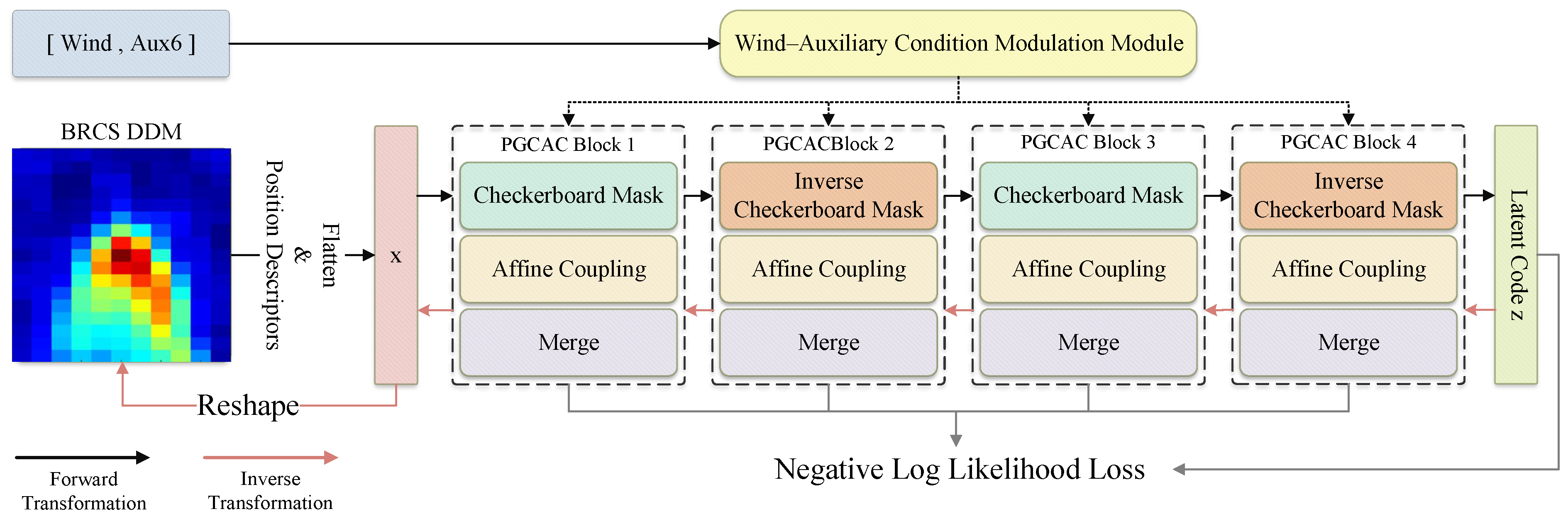
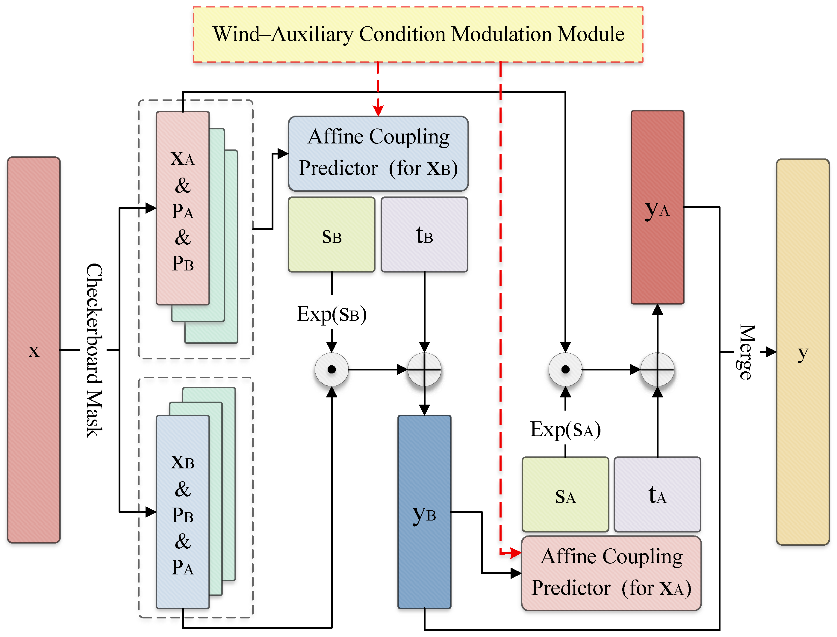
Figure 2 shows the four cascaded PGCAC Blocks. Each block uses the condition vector and fixed DDM-grid positions to predict cross-partition affine parameters. The blocks share the parameters of one Wind–Auxiliary Condition Modulation (WACM) module, while their remaining prediction layers are independent.

A normalized DDM $\mathbf{X}\in {\mathbb{R}}^{1\times 17\times 11}$ is flattened as $\mathbf{x}\in {\mathbb{R}}^{187}$, with each cell retaining a deterministic grid-position descriptor. Let $\mathbf{c}\in {\mathbb{R}}^7$ contain the normalized $U_{10}$ and six auxiliary variables. The forward mapping is

$$\mathbf{z}=f_{\mathsf{\Theta }}(\mathbf{x};\mathbf{c})=f_K\circ f_{K-1}\circ \cdots \circ f_1(\mathbf{x};\mathbf{c}),K=4$$

(13)

where $f_k$ is the kth PGCAC Block, $\mathsf{\Theta }$ denotes all learnable parameters, and $\mathbf{z}\in {\mathbb{R}}^{187}$ is the latent representation. The number of coupling blocks was fixed at four because the alternating sequence [CB, ICB, CB, ICB] provides two complete exchanges of the source and target roles between the complementary partitions. A single CB–ICB pair allows each partition to act once in each role, whereas the second pair repeats this interaction after the first pair has already transformed both partitions. Thus, four blocks provide repeated cross-partition interaction without introducing unnecessary flow depth. Increasing the number of blocks would repeat the same partition pattern while increasing computational cost, rather than introducing a new form of spatial interaction.

Because every block comprises analytically invertible affine transformations, no separate decoder is required:

$$\mathbf{x}=f_{\mathsf{\Theta }}^{-1}(\mathbf{z};\mathbf{c})=f_1^{-1}\circ f_2^{-1}\circ \cdots \circ f_K^{-1}(\mathbf{z};\mathbf{c})$$

(14)

The recovered vector is reshaped to 1 × 17 × 11. For a fixed recorded condition $\mathbf{c}$, the equal-dimensional mapping is one-to-one: forward evaluation maps an observed DDM to its latent representation, whereas ensemble generation maps independent latent samples through the inverse flow. The model is trained on the complete real training set, selected using the real validation set, and evaluated using held-out real test conditions.

In intuitive terms, each PGCAC Block performs a two-step exchange between two interleaved subsets of DDM cells. The checkerboard partition separates adjacent grid cells into complementary source and target subsets. The recorded wind and auxiliary conditions modulate the source-cell features, while the deterministic position descriptors determine how information from the source subset is aggregated for each target cell through PGCA. The resulting features are then used to predict the affine scale and translation parameters of the target subset. The two subsets subsequently exchange roles, so that both are updated within one block. Alternating the checkerboard assignment across successive blocks repeats this interaction between the complementary subsets while preserving the analytically invertible structure of the flow. Section 3.3, Section 3.4 and Section 3.5 provide the corresponding mathematical formulation.

3.3. DDM Grid Partition and Positional Descriptors

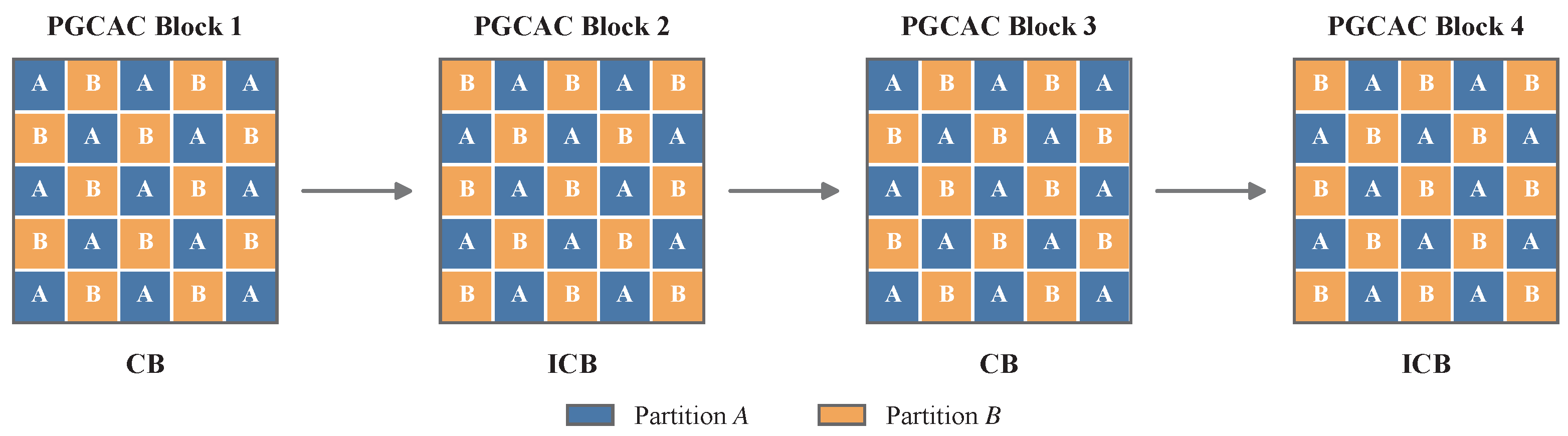
Each PGCAC Block applies two complementary affine transformations: one partition predicts the update of the other, after which the updated partition predicts the reverse update. As shown in Figure 3, the 17 × 11 grid is divided into two spatially interleaved subsets using the checkerboard (CB) mask

$$m_{ij}^{\mathrm{CB}}=\left\{\begin{array}{cc}1,\hfill & \mathrm{mod}(i+j,2)=0,\hfill \\ 0,\hfill & \mathrm{mod}(i+j,2)=1.\hfill \end{array}\right.$$

(15)

where $i=0,\dots ,16$ and $j=0,\dots ,10$. Values one and zero define partitions A and B, containing 94 and 93 cells, respectively; horizontally and vertically adjacent cells belong to different partitions.

The inverse checkerboard (ICB) mask exchanges the partition assignments:

$${\mathbf{M}}^{\mathrm{ICB}}=\mathbf{1}-{\mathbf{M}}^{\mathrm{CB}}$$

(16)

The four blocks alternate the masks as

$$\left[\mathrm{CB},\mathrm{ICB},\mathrm{CB},\mathrm{ICB}\right]$$

(17)

Thus, the two spatial subsets alternate their initial source–target roles across successive blocks.

Grid indices also provide deterministic positional descriptors that preserve cell locations after flattening. For cell $(i,j)$,

$${\mathbf{p}}_{ij}={\left[h,w,\Delta h,\Delta w,r,\Delta h^2,\Delta w^2,hw,\Delta h\Delta w\right]}^{\mathsf{T}}$$

(18)

Its components are defined in

Table 3. Nine-dimensional positional descriptors of the DDM cells.

Positional Component	Mathematical Definition	Descriptive Role
h	${\displaystyle \frac{i}{16}}$	Normalized absolute coordinate along the delay dimension
w	${\displaystyle \frac{j}{10}}$	Normalized absolute coordinate along the Doppler dimension
$\Delta h$	${\displaystyle \frac{i-8}{8}}$	Normalized delay-direction offset relative to the grid center
$\Delta w$	${\displaystyle \frac{j-5}{5}}$	Normalized Doppler-direction offset relative to the grid center
r	${\displaystyle \sqrt{\Delta h^2+\Delta w^2}}$	Radial distance in the normalized centered coordinate system
$\Delta h^2$	${\displaystyle {\left(\frac{i-8}{8}\right)}^2}$	Second-order positional feature along the delay dimension
$\Delta w^2$	${\displaystyle {\left(\frac{j-5}{5}\right)}^2}$	Second-order positional feature along the Doppler dimension
$hw$	${\displaystyle \frac{i}{16}\frac{j}{10}}$	Interaction between the normalized absolute coordinates
$\Delta h\Delta w$	${\displaystyle \frac{i-8}{8}\frac{j-5}{5}}$	Signed interaction between the delay- and Doppler-direction offsets

. The nine-dimensional descriptor was designed to provide a compact deterministic representation of complementary DDM-grid relationships. The absolute and center-relative coordinates retain cell location and direction, the radial term describes distance from the grid center, and the second-order and interaction terms provide simple nonlinear relationships between the delay and Doppler coordinates. This combination allows PGCA to distinguish cells using richer positional information than absolute grid coordinates alone, without introducing additional learned positional parameters. The effect of reducing this descriptor to simpler coordinate representations is examined in Section 4.7.

The row-major positional matrix is

$$\mathbf{P}={\left[{\mathbf{p}}_{00},\dots ,{\mathbf{p}}_{0,10},{\mathbf{p}}_{1,0},\dots ,{\mathbf{p}}_{16,10}\right]}^{\mathsf{T}}\in {\mathbb{R}}^{187\times 9}$$

(19)

The same ordered index sets ${\mathcal{I}}_A$ and ${\mathcal{I}}_B$ partition the DDM values and positional matrix:

$${\mathbf{x}}_A={\left[x_{ij}\right]}_{(i,j)\in {\mathcal{I}}_A},{\mathbf{x}}_B={\left[x_{ij}\right]}_{(i,j)\in {\mathcal{I}}_B}$$

(20)

$${\mathbf{P}}_A={\left[{\mathbf{p}}_{ij}^{\mathsf{T}}\right]}_{(i,j)\in {\mathcal{I}}_A},{\mathbf{P}}_B={\left[{\mathbf{p}}_{ij}^{\mathsf{T}}\right]}_{(i,j)\in {\mathcal{I}}_B}.$$

(21)

Under CB, $({\mathbf{x}}_A,{\mathbf{x}}_B)$ have dimensions (94, 93) and $({\mathbf{P}}_A,{\mathbf{P}}_B)$ have dimensions (94 × 9, 93 × 9); ICB exchanges these sizes. The fixed descriptors encode absolute, center-relative, radial, second-order, and interaction patterns on the DDM grid, rather than geographic coordinates or physical delay–Doppler values.

3.4. Position-Guided Conditional Affine Coupling Block

For block k, the mask partitions the input and its descriptors into $({\mathbf{x}}_A,{\mathbf{P}}_A)$ and $({\mathbf{x}}_B,{\mathbf{P}}_B)$. Let ${\mathsf{\theta }}_C$ denote the WACM parameters shared by all blocks and ${\mathsf{\theta }}_A^{\left(k\right)}$ and ${\mathsf{\theta }}_B^{\left(k\right)}$ the block-specific predictor parameters.

As shown in Figure 4, partition A first predicts the scale and translation parameters for partition B:

$$({\mathbf{s}}_B,{\mathbf{t}}_B)=g_{{\mathsf{\theta }}_B^{\left(k\right)},{\mathsf{\theta }}_C}\left({\mathbf{x}}_A,{\mathbf{P}}_A,{\mathbf{P}}_B,\mathbf{c}\right)$$

(22)

and partition B is updated as

$${\mathbf{y}}_B={\mathbf{x}}_B\odot \exp \left({\mathbf{s}}_B\right)+{\mathbf{t}}_B$$

(23)

Next, the updated ${\mathbf{y}}_B$ predicts the parameters of partition A:

$$({\mathbf{s}}_A,{\mathbf{t}}_A)=g_{{\mathsf{\theta }}_A^{\left(k\right)},{\mathsf{\theta }}_C}\left({\mathbf{y}}_B,{\mathbf{P}}_B,{\mathbf{P}}_A,\mathbf{c}\right)$$

(24)

with

$${\mathbf{y}}_A={\mathbf{x}}_A\odot \exp \left({\mathbf{s}}_A\right)+{\mathbf{t}}_A$$

(25)

The output partitions are restored to their original grid order:

$$\mathbf{y}=\mathrm{Merge}\left({\mathbf{y}}_A,{\mathbf{y}}_B;\mathbf{m}\right)$$

(26)

The inverse recomputes the same parameters in reverse order, recovering ${\mathbf{x}}_A$ from ${\mathbf{y}}_B$ and then ${\mathbf{x}}_B$ from the recovered ${\mathbf{x}}_A$:

$$\begin{array}{cc}\hfill ({\overline{\mathbf{s}}}_A,{\overline{\mathbf{t}}}_A)& =g_{{\mathsf{\theta }}_A^{\left(k\right)},{\mathsf{\theta }}_C}\left({\mathbf{y}}_B,{\mathbf{P}}_B,{\mathbf{P}}_A,\mathbf{c}\right),\hfill \\ \hfill {\mathbf{x}}_A& =\left({\mathbf{y}}_A-{\overline{\mathbf{t}}}_A\right)\odot \exp \left(-{\overline{\mathbf{s}}}_A\right),\hfill \\ \hfill ({\overline{\mathbf{s}}}_B,{\overline{\mathbf{t}}}_B)& =g_{{\mathsf{\theta }}_B^{\left(k\right)},{\mathsf{\theta }}_C}\left({\mathbf{x}}_A,{\mathbf{P}}_A,{\mathbf{P}}_B,\mathbf{c}\right),\hfill \\ \hfill {\mathbf{x}}_B& =\left({\mathbf{y}}_B-{\overline{\mathbf{t}}}_B\right)\odot \exp \left(-{\overline{\mathbf{s}}}_B\right).\hfill \end{array}$$

(27)

The barred quantities equal their forward counterparts under identical inputs; hence, the parameter predictors need not be invertible. The recovered partitions are finally merged:

$$\mathbf{x}=\mathrm{Merge}\left({\mathbf{x}}_A,{\mathbf{x}}_B;\mathbf{m}\right)$$

(28)

Because the scale values are bounded by the tanh function, the multiplicative factors remain between $e^{-1}$ and e, ensuring nonzero scaling and limiting numerical amplification during forward and inverse evaluation. Thus, each PGCAC Block updates both partitions while retaining an analytical inverse.

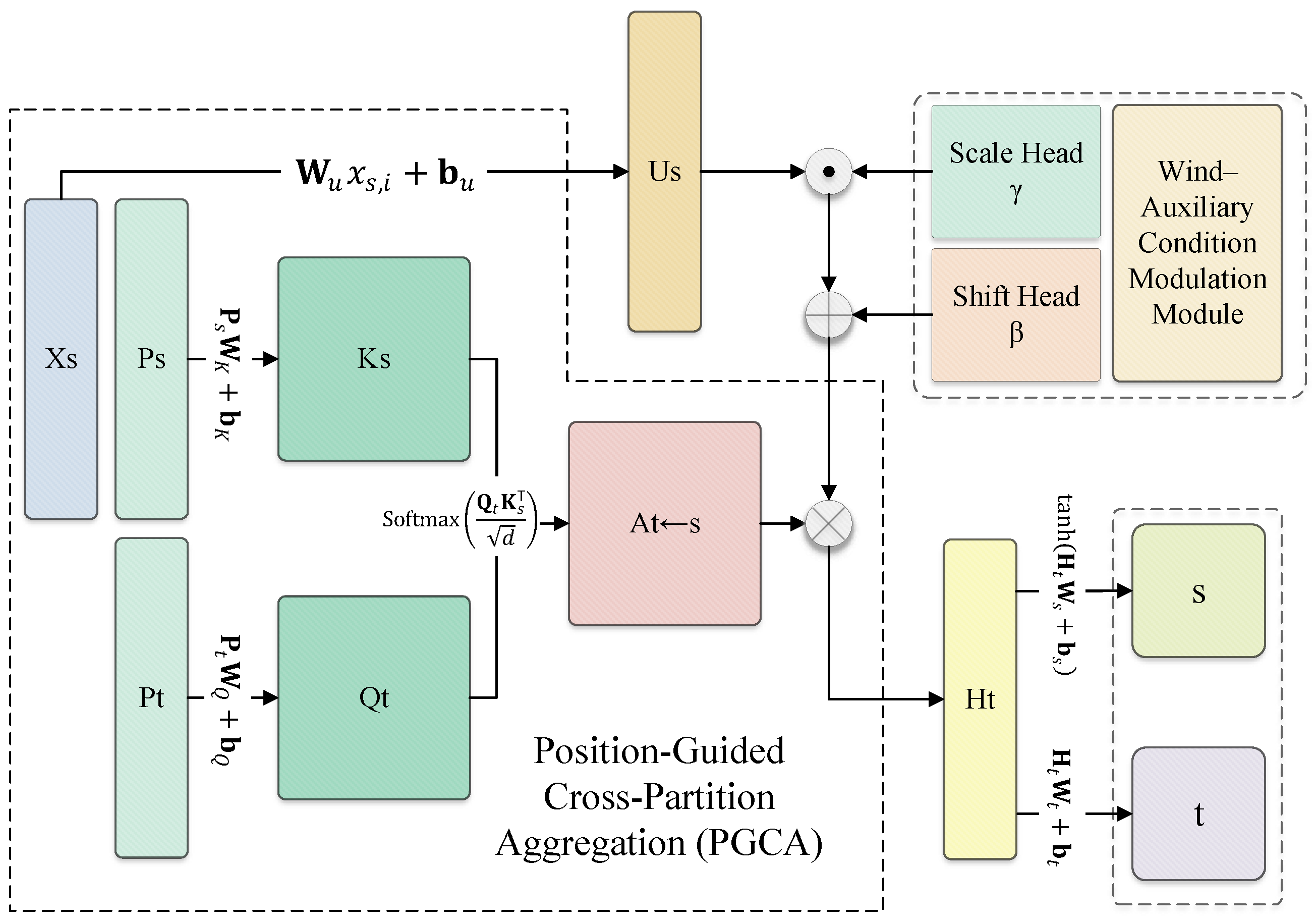
Figure 5 details the shared predictor structure. Denote the source and target partitions by ${\mathbf{x}}_s\in {\mathbb{R}}^{N_s}$ and ${\mathbf{x}}_t\in {\mathbb{R}}^{N_t}$, with descriptors ${\mathbf{P}}_s\in {\mathbb{R}}^{N_s\times 9}$ and ${\mathbf{P}}_t\in {\mathbb{R}}^{N_t\times 9}$. These correspond to $({\mathbf{x}}_A,{\mathbf{x}}_B)$ in the first transformation and $({\mathbf{y}}_B,{\mathbf{x}}_A)$ in the second. Each source value is embedded into $d=16$ dimensions:

$${\mathbf{u}}_i={\mathbf{W}}_u{x}_{s,i}+{\mathbf{b}}_u,{\mathbf{u}}_i\in {\mathbb{R}}^{16}$$

(29)

The internal feature dimension was set to $d=16$ for both the source-value embeddings and the positional key and query projections. In PGCA, this feature space serves primarily to bring the scalar DDM-cell values and the nine-dimensional positional descriptors into a common representation for cross-partition aggregation, rather than to construct a deep hierarchical image representation. Given the compact 17 × 11 DDM grid and the low-dimensional inputs involved in this interaction, $d=16$ provides a moderate intermediate representation while keeping the affine-parameter prediction structure compact.

Stacking the cell features gives

$${\mathbf{U}}_s={\left[{\mathbf{u}}_1,\dots ,{\mathbf{u}}_{N_s}\right]}^{\mathsf{T}}\in {\mathbb{R}}^{N_s\times 16}$$

(30)

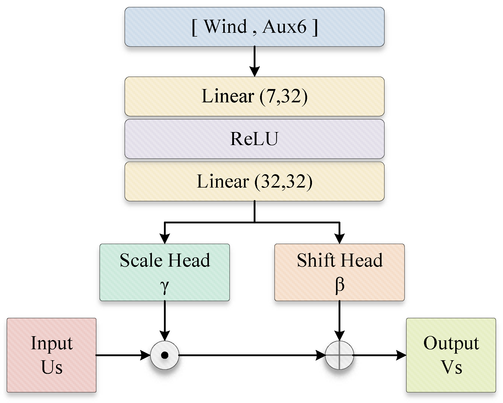
WACM injects the normalized wind speed and six auxiliary variables into the predictor (Figure 6). It adopts a feature-wise linear modulation (FiLM)-style affine operation [37]. Its shared two-layer multilayer perceptron encodes the seven-dimensional condition as

$${\mathbf{h}}_c=\varphi \left({\mathbf{W}}_{c1}\mathbf{c}+{\mathbf{b}}_{c1}\right)$$

(31)

$$\left[\begin{array}{c}\mathsf{\gamma }\\ \mathsf{\beta }\end{array}\right]={\mathbf{W}}_{c2}{\mathbf{h}}_c+{\mathbf{b}}_{c2}$$

(32)

where $\varphi$ is the ReLU activation. The $7\to 32\to 32$ encoder outputs $\mathsf{\gamma },\mathsf{\beta }\in {\mathbb{R}}^{16}$.

WACM applies feature-wise affine modulation to the source-partition value features:

$${\mathbf{V}}_s=(1+\mathsf{\gamma })\odot {\mathbf{U}}_s+\mathsf{\beta }$$

(33)

where broadcasting over cells gives ${\mathbf{V}}_s\in {\mathbb{R}}^{N_s\times 16}$. For a given condition, WACM provides the same $(\mathsf{\gamma },\mathsf{\beta })$ to every block, whereas the value embeddings, positional projections, and output heads remain block- and transformation-specific.

The source and target descriptors are projected into key and query spaces:

$${\mathbf{K}}_s={\mathbf{P}}_s{\mathbf{W}}_K+{\mathbf{b}}_K,{\mathbf{K}}_s\in {\mathbb{R}}^{N_s\times 16}$$

(34)

$${\mathbf{Q}}_t={\mathbf{P}}_t{\mathbf{W}}_Q+{\mathbf{b}}_Q,{\mathbf{Q}}_t\in {\mathbb{R}}^{N_t\times 16}$$

(35)

Following the scaled dot-product attention form [38], their cross-partition association is

$${\mathbf{A}}_{t\leftarrow s}=\mathrm{softmax}\left({\displaystyle \frac{{\mathbf{Q}}_t{\mathbf{K}}_s^{\mathsf{T}}}{\sqrt{d}}}\right),d=16$$

(36)

where ${\mathbf{A}}_{t\leftarrow s}\in {\mathbb{R}}^{N_t\times N_s}$ and softmax is applied over source cells. The modulated source features are aggregated as

$${\mathbf{H}}_t={\mathbf{A}}_{t\leftarrow s}{\mathbf{V}}_s,{\mathbf{H}}_t\in {\mathbb{R}}^{N_t\times 16}$$

(37)

Equations (34)–(37) constitute the Position-Guided Cross-Partition Aggregation (PGCA) module. PGCA aggregates the condition-modulated source-partition features for each target cell using association weights derived from deterministic source and target grid descriptors.

DDM values therefore provide the features, the condition modulates them, and grid positions determine the aggregation weights. Because the association matrix is derived from deterministic position descriptors rather than sample content, the operation is formulated as internal position-guided cross-partition attention rather than content-based self-attention; its output remains sample-dependent through ${\mathbf{U}}_s$. This design incorporates the fixed delay–Doppler grid geometry into affine-parameter prediction.

Separate heads produce

$$\mathbf{s}=\tanh \left({\mathbf{H}}_t{\mathbf{W}}_s+{\mathbf{b}}_s\right)$$

(38)

$$\mathbf{t}={\mathbf{H}}_t{\mathbf{W}}_t+{\mathbf{b}}_t$$

(39)

All matrices denoted by W are trainable linear projections used for feature embedding, condition encoding, position projection, or affine-parameter prediction. They are not required to be nonsingular because the invertibility of the overall model is ensured by the affine coupling transformation. Both vectors contain one parameter per target cell. The tanh function constrains $-1<s_i<1$, limiting exponential scaling and improving numerical stability. The target update is

$${\mathbf{y}}_t={\mathbf{x}}_t\odot \exp \left(\mathbf{s}\right)+\mathbf{t}$$

(40)

3.5. Jacobian Determinant and Loss Function

Because $\mathbf{s}$ and $\mathbf{t}$ depend only on the unchanged source partition, the log-Jacobian determinant of Equation (40) is

$$\log \left|\det \mathbf{J}\right|=\sum _i{s}_i$$

(41)

For the two transformations in one PGCAC Block,

$$\log \left|\det {\mathbf{J}}_{\mathrm{PGCAC}}\right|={\displaystyle \sum _{i=1}^{N_B}}{s}_{B,i}+{\displaystyle \sum _{j=1}^{N_A}}{s}_{A,j}$$

(42)

Here, $N_A$ and $N_B$ denote the numbers of cells in partitions A and B, respectively. Their values are (94, 93) under the CB mask and (93, 94) under the ICB mask, so each takes a value of either 93 or 94 and $N_A+N_B=187$. These values are fixed by the partition mask and do not change during training.

Across K blocks,

$$\log \left|\det {\mathbf{J}}_f\right|={\displaystyle \sum _{k=1}^K}\log \left|\det {\mathbf{J}}_{\mathrm{PGCAC}}^{\left(k\right)}\right|$$

(43)

For a mini-batch of B samples with ${\mathbf{z}}_n=f_{\mathsf{\Theta }}({\mathbf{x}}_n;{\mathbf{c}}_n)$, a standard Gaussian prior yields the conditional negative log-likelihood (excluding the parameter-independent constant):

$${\mathcal{L}}_{\mathrm{NLL}}={\displaystyle \frac{1}{B}}{\displaystyle \sum _{n=1}^B}\left[{\displaystyle \frac{1}{2}}{∥{\mathbf{z}}_n∥}_2^2-\log \left|\det {\mathbf{J}}_f({\mathbf{x}}_n;{\mathbf{c}}_n)\right|\right]$$

(44)

3.6. Recorded-Condition Ensemble Sampling

After training, DDM ensembles are generated under a standardized recorded condition vector

$${\mathbf{c}}_i={\left[{\tilde{U}}_{10,i},{\tilde{\mathbf{a}}}_i^{\mathsf{T}}\right]}^{\mathsf{T}},$$

(45)

where ${\tilde{U}}_{10,i}$ is the standardized ERA5 10 m wind speed and ${\tilde{\mathbf{a}}}_i$ is the corresponding standardized six-dimensional auxiliary vector. For ensemble member k, a latent vector is independently sampled from the standard Gaussian prior:

$${\mathbf{z}}_i^{\left(k\right)}\sim \mathcal{N}\left(\mathbf{0},{\mathbf{I}}_{187}\right)$$

(46)

The sampled latent vector is then mapped through the inverse conditional flow:

$${\tilde{\mathbf{x}}}_i^{\left(k\right)}=f_{\mathsf{\Theta }}^{-1}\left({\mathbf{z}}_i^{\left(k\right)};{\mathbf{c}}_i\right)$$

(47)

Repeating Equations (46) and (47) for $k=1,\dots ,K$ yields the expanded ensemble

$${\mathcal{E}}_i^{\mathrm{PGCFlow}}=\left\{{\tilde{\mathbf{x}}}_i^{\left(1\right)},{\tilde{\mathbf{x}}}_i^{\left(2\right)},\dots ,{\tilde{\mathbf{x}}}_i^{\left(K\right)}\right\}$$

(48)

Each generated vector is reshaped into a 1 × 17 × 11 DDM and inverse-standardized to the original BRCS scale using the training-set statistics. The associated condition is retained, producing the generated pairs

$${\left\{\left({\mathbf{c}}_i,{\tilde{\mathbf{x}}}_i^{\left(k\right)}\right)\right\}}_{k=1}^K$$

(49)

In the experiments, ${\mathbf{c}}_i$ is always a condition vector attached to a held-out real test observation rather than an arbitrarily constructed condition combination. The matched real DDM is used as an evaluation reference but is not an input to the inverse-generation operation. Variation across ${\mathcal{E}}_i^{\mathrm{PGCFlow}}$ is interpreted as residual variability relative to the seven selected conditioning variables; individual latent dimensions are not assigned to specific unresolved physical or instrumental factors.

4. Results and Discussion

This section evaluates whether observation-conditioned generation expands a single condition–DDM pairing into an ensemble that retains relevant characteristics of the real observations. Because only one real DDM is available for each exact recorded condition, no single metric can verify the unobserved true conditional distribution. The evaluation therefore uses four complementary evidence layers: single-reference structural fidelity, ensemble-level quality, dispersion relative to a local real-neighborhood proxy, and wind-speed responses under an independently trained frozen DDM-only estimator. The evidence is interpreted separately at each layer and is restricted to held-out real conditions from the empirical data domain. In addition, numerical invertibility and basic marginal statistics of the learned latent representation are examined as flow-specific diagnostics.

4.1. Experimental Setup

4.1.1. Compared Models

PGCFlow was compared with two conditional generative baselines: a conditional variational autoencoder (cVAE) [26] and a conditional invertible neural network (cINN) [36]. The cVAE models the conditional distribution through a stochastic low-dimensional latent variable and a decoder, whereas cINN and PGCFlow learn invertible mappings between the DDM and an equal-dimensional Gaussian latent space. The cINN serves as a generic conditional normalizing-flow baseline without the Wind–Auxiliary Condition Modulation (WACM) and Position-Guided Cross-Partition Aggregation (PGCA) mechanisms used within the PGCAC Blocks of PGCFlow. All three models used identical data splits, seven-dimensional conditions, training-set normalization statistics, and validation-based checkpoint selection, and generated single-channel 17 × 11 BRCS DDMs for the same test conditions.

The cVAE used a 64-dimensional learned conditional Gaussian prior rather than a condition-independent standard normal prior.

Table 4. Architecture of the conditional VAE baseline.

Component	Input	Hidden Dimensions	Operation	Output
Posterior encoder	187 + 7	512, 256	Flatten DDM, concatenate condition, and use two parameter heads	${\mathsf{\mu }}_q,\log {\mathsf{\sigma }}_q^2\in {\mathbb{R}}^{64}$
Conditional prior	7	128, 128	Encode condition and use two parameter heads	${\mathsf{\mu }}_p,\log {\mathsf{\sigma }}_p^2\in {\mathbb{R}}^{64}$
Decoder	64 + 7	$256,512$	Concatenate latent vector and condition; linear output; reshape	1 × 17 × 11

summarizes its implemented architecture. Each hidden fully connected layer used LayerNorm and GELU, and the dropout rate was zero. The posterior and prior log-variances were clipped to $[-12,8]$.

The cINN flattened each DDM into a 187-dimensional vector and transformed it into a latent vector of the same dimension. It consisted of four bidirectional conditional affine coupling blocks. Each block first applied a fixed random permutation and then divided the vector into two partitions of 94 and 93 elements. Two successive affine transformations updated both partitions, with the seven-dimensional condition directly concatenated to the corresponding coupling-subnetwork input. Each coupling subnetwork contained two fully connected hidden layers with 256 units and ReLU activation. The logarithmic scale was bounded using a hyperbolic tangent function with a clamp value of 1, and dropout was not used.

Table 5. Structural summary of the conditional invertible neural network baseline.

Component	Configuration	Description
Input and latent space	$187\leftrightarrow 187$	The single-channel 17 × 11 DDM is flattened and mapped invertibly to an equal-dimensional latent vector.
Flow structure	Four blocks	Each block applies a fixed random permutation followed by two conditional affine coupling transformations.
Partition scheme	94 + 93	The input vector is divided into two complementary partitions that are updated successively within each block.
Coupling subnetworks	256, 256	Two fully connected hidden layers with ReLU activation predict the affine scale and translation parameters.
Conditioning	Seven dimensions	The condition vector is directly concatenated with the active partition of each coupling transformation.

summarizes its implemented architecture. Unlike PGCFlow, the cINN contained no explicit position encoding, Position-Guided Cross-Partition Aggregation, or feature-wise condition-modulation mechanism.

4.1.2. Training Details

Experiments were implemented in Python 3.9 using PyTorch 2.7.1 and CUDA 12.8, and were conducted on an NVIDIA RTX 5070 GPU. Architectural settings were specified according to the formulation of each model, while common optimization settings were kept consistent across models whenever applicable. In PGCFlow, $d=16$ was adopted as a compact intermediate feature dimension for the cell-value and positional representations, while four alternating CB–ICB coupling blocks provide two complete source–target exchange cycles between the complementary partitions.

All three generators were trained independently for up to 60 epochs with a batch size of 1024, Adam ($\mathrm{lr}={10}^{-4}$, zero weight decay), and gradient clipping at 5.0. Each model was trained independently with ten random seeds (from 2021 to 2030), and the run with the lowest validation loss was selected for final evaluation. The learning rate was halved after four consecutive validation epochs without improvement, down to a minimum of ${10}^{-6}$, and training was stopped when the validation loss failed to improve for ten consecutive epochs. Validation loss controlled scheduling, early stopping, and checkpoint selection; the test set remained unused.

The computational characteristics of the three generative models are summarized in

Table 6. Computational characteristics of the compared generative models.

Model	Trainable Parameters	Estimated Compute Time per Epoch (min)	Batched Generation Time (ms/Condition, $\mathit{K}=16$)
cVAE	547,643	0.1643	0.00245
cINN	1,118,680	0.3100	0.00976
PGCFlow	12,304	0.6826	0.02448

. PGCFlow has 12,304 trainable parameters, compared with 547,643 for the cVAE and 1,118,680 for the cINN. The larger parameter count of the cVAE mainly results from its encoder and decoder with hidden dimensions of 512 and 256, together with the additional conditional prior network. The cINN contains still more parameters because each of its four coupling blocks uses two multilayer perceptrons with 256 hidden units. In contrast, PGCFlow uses a 16-dimensional feature representation and a 32-dimensional condition modulation network within its coupling structure, which keeps the number of trainable parameters relatively small. This compact parameterization does not, however, translate directly into lower computational latency, because the structured positional operations in PGCFlow introduce additional computation. Under the same hardware and batch settings, the estimated computation time per epoch was 0.6826 min for PGCFlow, compared with 0.1643 min for the cVAE and 0.3100 min for the cINN. For batched generation with $K=16$ DDMs per condition, the corresponding generation times were 0.02448, 0.00245, and 0.00976 ms/condition for PGCFlow, cVAE, and cINN, respectively. The timing measurements exclude data loading, CPU preprocessing, device transfer, checkpoint writing, and other file I/O.

For the cVAE, the reconstruction and KL terms had target weights of one, with the KL weight linearly increased during the first 20 epochs. Its negative conditional ELBO loss was

$${\mathcal{L}}_{\mathrm{cVAE}}={\displaystyle \frac{1}{B}}{\displaystyle \sum _{n=1}^B}\left[{\displaystyle \frac{1}{2}}{∥{\mathbf{x}}_n-{\widehat{\mathbf{x}}}_n∥}_2^2+\beta D_{\mathrm{KL}}\left(q_{\varphi }\left(\mathbf{z}\mid {\mathbf{x}}_n,{\mathbf{c}}_n\right)\parallel p_{\psi }\left(\mathbf{z}\mid {\mathbf{c}}_n\right)\right)\right]$$

(50)

The cINN was optimized using the same conditional negative log-likelihood formulation as PGCFlow. For a mini-batch of B samples, its loss was

$${\mathcal{L}}_{\mathrm{cINN}}={\displaystyle \frac{1}{B}}{\displaystyle \sum _{n=1}^B}\left[{\displaystyle \frac{1}{2}}{∥{\mathbf{z}}_n∥}_2^2-\log \left|\det {\displaystyle \frac{\partial f_{\theta }\left({\mathbf{x}}_n;{\mathbf{c}}_n\right)}{\partial {\mathbf{x}}_n}}\right|\right],{\mathbf{z}}_n=f_{\theta }\left({\mathbf{x}}_n;{\mathbf{c}}_n\right)$$

(51)

where the parameter-independent Gaussian constant was omitted. The cINN and PGCFlow therefore share the same likelihood objective, but differ in the construction of their conditional invertible transformations.

4.1.3. Conditional Sampling Procedure

All generation conditions were drawn from recorded condition vectors in the held-out test split and were not used for model fitting or checkpoint selection. Each condition vector was associated with a real observation rather than a synthetically constructed combination. Using a fixed random seed, 2000 test conditions were sampled without replacement from each of four wind-speed intervals,

$$[0,5),[5,10),[10,15),[15,+\infty )\mathrm{m}/\mathrm{s}$$

(52)

giving 8000 conditions in total. For every condition, each model independently generated $K=16$ DDMs from its prior, resulting in 128,000 generated samples per model. This balanced evaluation design gives equal weight to all four wind-speed strata; it does not reproduce the natural frequency distribution of the complete test set.

For the cVAE, the conditional-prior network produced ${\mathsf{\mu }}_p\left(\mathbf{c}\right)$ and ${\mathsf{\sigma }}_p\left(\mathbf{c}\right)$, and each member was sampled as

$$\mathsf{ϵ}\sim \mathcal{N}(\mathbf{0},{\mathbf{I}}_{64}),{\mathbf{z}}_{\mathrm{VAE}}={\mathsf{\mu }}_p\left(\mathbf{c}\right)+{\mathsf{\sigma }}_p\left(\mathbf{c}\right)\odot \mathsf{ϵ}$$

(53)

$${\tilde{\mathbf{X}}}_{\mathrm{cVAE}}=g_{\theta }({\mathbf{z}}_{\mathrm{VAE}},\mathbf{c})$$

(54)

For the two flow-based models, each ensemble member was generated as

$${\mathbf{z}}_m\sim \mathcal{N}\left(\mathbf{0},{\mathbf{I}}_{187}\right),{\tilde{\mathbf{x}}}_m=f_m^{-1}\left({\mathbf{z}}_m;\mathbf{c}\right),m\in \left\{\mathrm{cINN},\mathrm{PGCFlow}\right\}.$$

(55)

Outputs from all three models were reshaped into single-channel 1 × 17 × 11 DDMs and inverse-standardized to the original BRCS scale using the training-set statistics. Repeated latent sampling under the same seven-dimensional recorded condition produced an expanded ensemble representing variability not explained by the selected conditioning variables. Because the conditions came from held-out observations drawn under the same source and preprocessing definitions as the training data, the experiment tests expansion at recorded conditions rather than extrapolation to an unobserved condition domain.

4.2. Representative Expanded DDM Ensembles

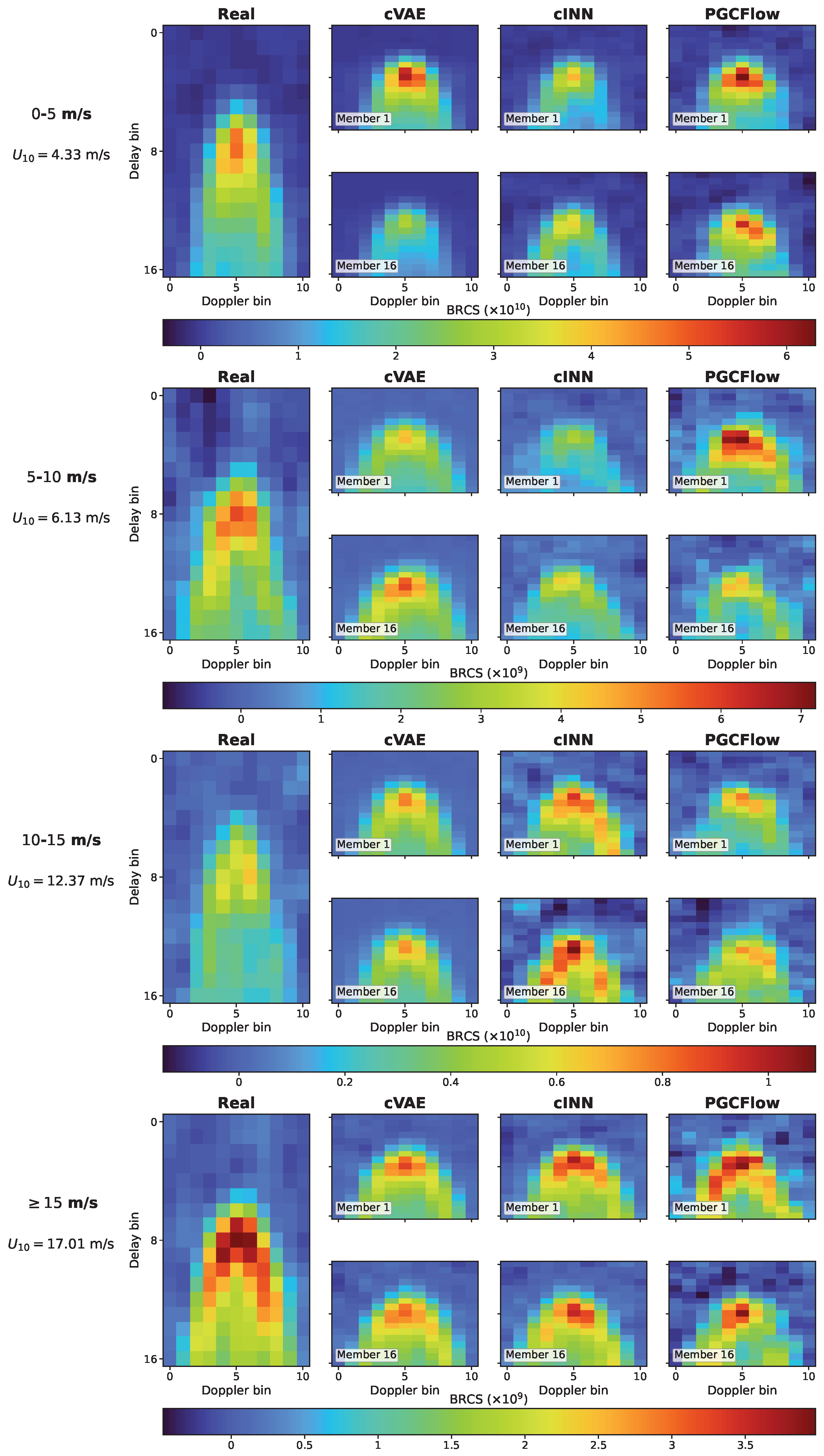
To qualitatively examine the generated DDMs, one conditioning sample was randomly selected from each of the four wind-speed subsets using a fixed random seed. For each selected condition, the corresponding real DDM was compared with Members 1 and 16 from the 16-member ensembles generated by cVAE, cINN and PGCFlow. All DDMs are presented on the original BRCS scale without interpolation or value clipping. Within each row, the real and generated DDMs share a common color range, enabling direct comparison of their intensity distributions. The vertical and horizontal directions correspond to the delay and Doppler bins, respectively.

Figure 7 provides a qualitative view of the single-reference structure and within-ensemble variation produced by the three generators. The correspondence between each generated DDM and its matched real DDM can be examined in terms of peak intensity and location, delay–Doppler spreading, and local scattering patterns. The two displayed members from each generator allow qualitative inspection of within-ensemble variation. These selected examples are descriptive rather than distributional evidence and are therefore interpreted together with the condition-aggregated metrics below.

4.3. Evaluation Framework and Metrics

Table 7. Complementary quantitative measures used to assess the expanded DDM ensembles.

Metric	Evaluation Type	Quantity Evaluated	Preferred	Brief Interpretation
SSIM	Single-reference fidelity	Local DDM structure	Higher	Similarity to the one condition-matched real DDM
FES	Ensemble-level quality	Proximity and dispersion	Lower	Proper multivariate score for the generated ensemble
VS	Ensemble-level quality	Inter-cell dependence	Lower	Agreement of delay–Doppler inter-cell variation patterns
$R_{\mathrm{LND}}$	Local-neighborhood proxy	Relative ensemble dispersion	Closer to 1	Dispersion relative to a selected local real-neighborhood proxy

summarizes four complementary metrics: structural similarity (SSIM), the Fair Energy Score (FES), the Variogram Score (VS), and relative local-neighborhood dispersion ($R_{\mathrm{LND}}$). The measures answer different questions and are not combined into a single composite ranking: SSIM concerns similarity to one observed realization, FES and VS concern the quality of the generated ensemble, and $R_{\mathrm{LND}}$ compares its dispersion with an empirical local-neighborhood proxy. Let ${\mathbf{x}}_n\in {\mathbb{R}}^P$ denote the normalized real DDM associated with test condition n, and let ${\tilde{\mathbf{x}}}_{n,k}$, $k=1,\dots ,K$, denote the corresponding generated DDMs, where $P=17\times 11=187$ and $K=16$. The distance between two normalized DDMs was defined as

$$d(\mathbf{a},\mathbf{b})=\sqrt{{\displaystyle \frac{1}{P}}\sum _{p=1}^P{(a_p-b_p)}^2}$$

(56)

Structural similarity (SSIM) measures the luminance, contrast, and structural agreement between a generated DDM and its condition-matched real counterpart [39]:

$$\mathrm{SSIM}(\mathbf{x},\tilde{\mathbf{x}})={\displaystyle \frac{(2{\mu }_{\mathbf{x}}{\mu }_{\tilde{\mathbf{x}}}+C_1)(2{\sigma }_{\mathbf{x}\tilde{\mathbf{x}}}+C_2)}{({\mu }_{\mathbf{x}}^2+{\mu }_{\tilde{\mathbf{x}}}^2+C_1)({\sigma }_{\mathbf{x}}^2+{\sigma }_{\tilde{\mathbf{x}}}^2+C_2)}}$$

(57)

The local means, variances, and covariance were computed in the normalized DDM space using a 7 × 7 uniform window, reflection padding, and sample-covariance correction, and the resulting SSIM map was spatially averaged. The constants were $C_1={\left(0.01L\right)}^2$ and $C_2={\left(0.03L\right)}^2$, where L was the global value range of the 8000 real reference DDMs sampled evenly across the four wind-speed intervals. The same L was used for all images and models. Higher SSIM indicates greater fidelity to the matched reference. Because that reference is only one realization under the finite condition representation, SSIM does not measure coverage of the full conditional distribution.

Ensemble quality was assessed using the Fair Energy Score (FES) and Variogram Score (VS). The energy score is a proper multivariate scoring rule that jointly accounts for accuracy and dispersion [40]. Its finite-ensemble fair form corrects the ensemble-size bias in the pairwise term [41]:

$${\mathrm{FES}}_n={\displaystyle \frac{1}{K}}{\displaystyle \sum _{k=1}^K}d({\tilde{\mathbf{x}}}_{n,k},{\mathbf{x}}_n)-{\displaystyle \frac{1}{2\left(\genfrac{}{}{0pt}{}{K}{2}\right)}}\sum _{1\le k<l\le K}d({\tilde{\mathbf{x}}}_{n,k},{\tilde{\mathbf{x}}}_{n,l})$$

(58)

The VS complements the FES by emphasizing the spatial dependence between DDM cells [42]:

$${\mathrm{VS}}_n=\sum _{i<j}{w}_{ij}{\left[|x_{n,i}-x_{n,j}{|}^q-{\displaystyle \frac{1}{K}}{\displaystyle \sum _{k=1}^K}{|{\tilde{x}}_{n,k,i}-{\tilde{x}}_{n,k,j}|}^q\right]}^2$$

(59)

where $q=0.5$ and $w_{ij}=r_{ij}^{-1}/{\sum }_{u<v}{r}_{uv}^{-1}$, with $r_{ij}$ denoting the grid distance between cells i and j. All $\left({\displaystyle \genfrac{}{}{0pt}{}{187}{2}}\right)=$ 17,391 cell pairs were included. Lower FES and VS values indicate better ensemble quality. These scores are calculated for each condition using its observed DDM as the verifying realization and are then aggregated across the evaluation conditions.

Following the pairwise-distance approach commonly used to evaluate the diversity of multiple conditional outputs [43,44], generated-ensemble dispersion was measured by averaging the pairwise distances defined in (56). For each condition n, the generated dispersion was calculated as

$$D_n^{\mathrm{gen}}={\displaystyle \frac{2}{K(K-1)}}\sum _{1\le k<l\le K}d({\tilde{\mathbf{x}}}_{n,k},{\tilde{\mathbf{x}}}_{n,l})$$

(60)

Because repeated observations under an identical and complete observing state were unavailable, a local real-neighborhood proxy was constructed for each target condition. Let ${\mathcal{T}}_b$ denote the complete test-set candidate pool in wind-speed interval b. The target sample itself was removed from ${\mathcal{T}}_b$ before Euclidean distances were computed in the standardized seven-dimensional condition space. The 15 nearest remaining test conditions were then selected and combined with the target real DDM to form a 16-member local proxy. Training and validation samples were not eligible neighbors. Denoting these real DDMs by ${\mathbf{x}}_{n,k}^{\mathrm{loc}}$, their dispersion was calculated as

$$D_n^{\mathrm{real}}={\displaystyle \frac{2}{K(K-1)}}\sum _{1\le k<l\le K}d({\mathbf{x}}_{n,k}^{\mathrm{loc}},{\mathbf{x}}_{n,l}^{\mathrm{loc}})$$

(61)

Both dispersions therefore represent the mean of $K(K-1)/2=120$ within-set pairwise distances. For a set of evaluated conditions $\mathcal{S}$, the relative local-neighborhood dispersion was defined as

$$R_{\mathrm{LND}}\left(\mathcal{S}\right)={\displaystyle \frac{{\sum }_{n\in \mathcal{S}}{D}_n^{\mathrm{gen}}}{{\sum }_{n\in \mathcal{S}}{D}_n^{\mathrm{real}}}}$$

(62)

Here, $\mathcal{S}$ denotes either a wind-speed interval or the complete evaluation set. A value close to one indicates that the generated ensemble produced dispersion comparable to the selected local real-neighborhood proxy, whereas values below or above one indicate lower or greater relative dispersion, respectively. The proxy members have nearby, rather than identical, recorded conditions. Accordingly, $R_{\mathrm{LND}}$ is an empirical comparison of local dispersion and not an estimate of the variance under an exactly repeated complete observing state.

For the validation-selected runs, statistical uncertainty was quantified using 2000 condition-level bootstrap resamples. In each replicate, parent test conditions were sampled with replacement, while all 16 generated members associated with each selected condition were retained. For pairwise model comparisons, the same resampled condition indices were applied to both models, forming a paired bootstrap. For model-specific metrics, each metric was recomputed directly from the resampled conditions. The 2.5th and 97.5th percentiles of the bootstrap distributions define the reported 95% confidence intervals. These intervals characterize uncertainty associated with the finite test cohort for the selected runs. The ≥15 m/s interval contained 45,191 observations in the complete dataset and 6615 observations in the test split, from which 2000 conditions were used in the equal-bin evaluation. The reported bootstrap intervals quantify uncertainty associated with resampling these evaluated conditions, but they do not compensate for the limited coverage of the broader high-wind condition space.

4.4. Single-Reference Structural Fidelity and Ensemble-Level Quality

Because each wind-speed interval contributed the same number of test conditions, the balanced aggregate assigns equal weight to the four wind-speed intervals. For SSIM, FES, and VS, this is equivalent to the arithmetic mean of the four interval-wise results.

For each model, the reported point estimates correspond to the run with the lowest validation loss among ten independently initialized training runs. Pairwise differences are defined as $\Delta =\mathrm{candidate}-\mathrm{PGCFlow}$, and the reported 95% confidence intervals were obtained from 2000 condition-level paired bootstrap resamples of the selected runs.

Table 8. Single-reference fidelity and ensemble-level quality of the compared models.

Wind Bin	Model	SSIM ↑		FES ↓		VS ↓
		Value	Δ [95% CI]	Value	Δ [95% CI]	Value	Δ [95% CI]
0–5	cVAE	0.8832	$-0.0131[-0.0152,-0.0108]$	0.3496	$-0.0162[-0.0214,-0.0110]$	0.0922	$0.0021[-0.0001,0.0044]$
	cINN	0.8609	$-0.0354[-0.0384,-0.0327]$	0.3680	$0.0022[-0.0058,0.0105]$	0.0928	$0.0027[-0.0010,0.0064]$
	PGCFlow	0.8963	Reference	0.3657	Reference	0.0901	Reference
5–10	cVAE	0.9491	$0.0124[0.0109,0.0140]$	0.2015	$0.0075[0.0053,0.0097]$	0.0657	$0.0086[0.0064,0.0108]$
	cINN	0.9173	$-0.0194[-0.0217,-0.0171]$	0.1955	$0.0015[-0.0015,0.0045]$	0.0607	$0.0036[0.0008,0.0069]$
	PGCFlow	0.9366	Reference	0.1939	Reference	0.0570	Reference
10–15	cVAE	0.9612	$0.0157[0.0140,0.0174]$	0.1844	$0.0123[0.0103,0.0142]$	0.0661	$0.0112[0.0086,0.0142]$
	cINN	0.9413	$-0.0042[-0.0063,-0.0022]$	0.1742	$0.0021[-0.0002,0.0049]$	0.0607	$0.0058[0.0023,0.0096]$
	PGCFlow	0.9455	Reference	0.1721	Reference	0.0549	Reference
≥15	cVAE	0.9651	$0.0214[0.0191,0.0236]$	0.1833	$0.0184[0.0156,0.0215]$	0.0714	$0.0171[0.0126,0.0224]$
	cINN	0.9543	$0.0106[0.0083,0.0129]$	0.1734	$0.0084[0.0049,0.0127]$	0.0665	$0.0122[0.0065,0.0193]$
	PGCFlow	0.9437	Reference	0.1649	Reference	0.0542	Reference
Balanced aggregate	cVAE	0.9396	$0.0091[0.0081,0.0101]$	0.2297	$0.0055[0.0038,0.0071]$	0.0738	$0.0098[0.0083,0.0114]$
	cINN	0.9184	$-0.0121[-0.0133,-0.0108]$	0.2277	$0.0036[0.0011,0.0061]$	0.0702	$0.0061[0.0040,0.0084]$
	PGCFlow	0.9305	Reference	0.2242	Reference	0.0641	Reference

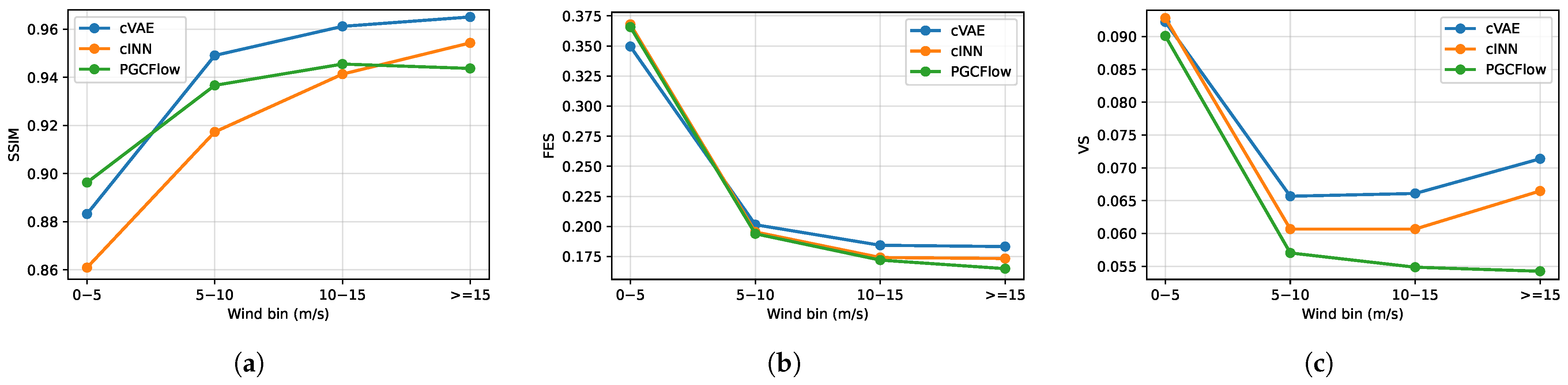
Note: Upward and downward arrows indicate better performance for higher and lower values, respectively. Bold values indicate the best performance for each metric.

and Figure 8 show distinct model behavior at the single-reference and ensemble levels. In the balanced aggregate, the cVAE achieved the highest SSIM of 0.9396, followed by PGCFlow at 0.9305 and cINN at 0.9184. This indicates that the cVAE generated samples with the greatest average structural similarity to the matched real DDM. In contrast, PGCFlow obtained the lowest FES and VS, with values of 0.2242 and 0.0641, respectively. The cINN achieved intermediate FES and VS values of 0.2277 and 0.0702, improving upon the cVAE but remaining less favorable than PGCFlow.

The interval-wise results show a similar tradeoff. In the 0–5 m/s interval, PGCFlow achieved the highest SSIM and lowest VS, whereas the cVAE obtained the lowest FES. The cINN did not outperform the other two models in this interval. Above 5 m/s, Table 8 reveals a metric-dependent trade-off among the three generative models. In the 0–5 m/s interval, PGCFlow achieved the highest SSIM, with paired 95% confidence intervals supporting its advantage over both the cVAE and cINN. In the 5–10 and 10–15 m/s intervals, the cVAE retained the highest SSIM, whereas PGCFlow achieved the lowest VS, with its advantages over both baselines supported by the paired bootstrap intervals. PGCFlow also obtained a significantly lower FES than the cVAE in both intervals. In the ≥15 m/s interval, PGCFlow achieved the lowest FES and VS, and the paired confidence intervals confirmed its advantages over both baselines for both ensemble-level metrics. Although some smaller differences, such as the FES difference between cINN and PGCFlow in the intermediate wind-speed intervals, were not clearly separated, the interval-wise bootstrap analysis shows that several of the advantages of PGCFlow are supported beyond the point estimates.

For the balanced aggregate, the cVAE retained a higher SSIM than PGCFlow, with a paired difference of 0.0091 (95% CI: $[0.0081,0.0101]$). In contrast, PGCFlow obtained lower FES than both the cVAE and cINN, with paired differences of 0.0055 (95% CI: $[0.0038,0.0071]$) and 0.0036 (95% CI: $[0.0011,0.0061]$), respectively. The corresponding VS differences were 0.0098 (95% CI: $[0.0083,0.0114]$) and 0.0061 (95% CI: $[0.0040,0.0084]$), and all four intervals excluded zero. These results indicate that the models emphasize different aspects of conditional generation: the cVAE generally favors single-reference similarity, whereas PGCFlow provides stronger ensemble-level proximity and spatial-dependence scores.

One possible contributor to the higher cVAE SSIM is its learned conditional Gaussian prior, which adapts the latent distribution to the recorded condition, whereas cINN and PGCFlow sample from a fixed standard Gaussian prior and introduce the condition through the invertible transformation. Together with the reconstruction term in the cVAE objective, this design may favor samples that remain closer to the matched realization, which benefits a single-reference metric such as SSIM. This interpretation does not attribute the SSIM difference to the prior alone, since the models also differ in their overall architectures and training objectives.

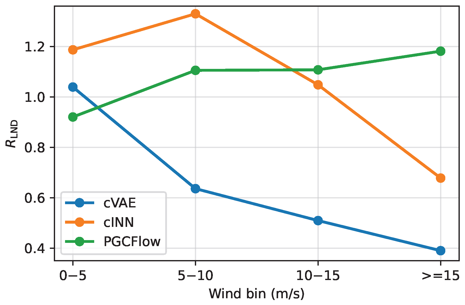
4.5. Local-Neighborhood Diversity Proxy

Table 9. Relative local-neighborhood dispersion of the expanded ensembles.

Wind Bin	Model	RLND	$|\mathbf{RLND}-1|$	Δ$|\mathbf{RLND}-1|$ [95% CI]
0–5	cVAE	1.0391	0.0391	$-0.0406[-0.1026,0.0265]$
	cINN	1.1867	0.1867	$0.1070[0.0443,0.1726]$
	PGCFlow	0.9203	0.0797	Reference
5–10	cVAE	0.6361	0.3639	$0.2586[0.1905,0.3266]$
	cINN	1.3296	0.3296	$0.2243[0.1697,0.2816]$
	PGCFlow	1.1053	0.1053	Reference
10–15	cVAE	0.5095	0.4905	$0.3831[0.3031,0.4584]$
	cINN	1.0478	0.0478	$-0.0596[-0.1058,-0.0085]$
	PGCFlow	1.1074	0.1074	Reference
≥15	cVAE	0.3901	0.6099	$0.4286[0.3493,0.5066]$
	cINN	0.6780	0.3220	$0.1407[0.0572,0.2184]$
	PGCFlow	1.1813	0.1813	Reference
Balanced aggregate	cVAE	0.7166	0.2834	$0.2334[0.1979,0.2693]$
	cINN	1.0926	0.0926	$0.0425[0.0181,0.0679]$
	PGCFlow	1.0501	0.0501	Reference

Note: Bold values indicate the best performance for each metric.

reports $R_{\mathrm{LND}}$ and its absolute deviation from unity. In the 0–5 m/s interval, the cVAE produced the closest point estimate, although its paired difference from PGCFlow included zero. PGCFlow was closest to unity in the 5–10 m/s interval, whereas cINN was closest in the 10–15 m/s interval. In the ≥15 m/s interval, PGCFlow obtained the closest point estimate, and its paired intervals against both baselines excluded zero; however, this result is treated as cohort-specific because of the limited high-wind coverage. For the balanced aggregate, PGCFlow achieved the smallest absolute deviation from unity, with an $R_{\mathrm{LND}}$ of 1.0501, and its advantage over both baselines was supported by the paired bootstrap intervals.

For each model, the reported point estimates correspond to the run with the lowest validation loss among ten independently initialized training runs. Pairwise differences are defined as $\Delta |\mathrm{RLND}-1|=|{\mathrm{RLND}}_{\mathrm{candidate}}-1|-|{\mathrm{RLND}}_{\mathrm{PGCFlow}}-1|$, and the 95% confidence intervals were obtained from 2000 condition-level paired bootstrap resamples.

The aggregate $R_{\mathrm{LND}}$ was calculated as the ratio between the pooled generated and local-real dispersion sums, rather than as the average of the four interval-wise ratios (Figure 9). The cVAE yielded an $R_{\mathrm{LND}}$ of 0.7166, indicating overall dispersion contraction, whereas cINN produced 1.0926, indicating mild overdispersion. PGCFlow achieved the closest aggregate value to unity at 1.0501. Thus, the generic invertible cINN substantially alleviated the contraction observed for the cVAE, while PGCFlow provided the most balanced local-dispersion calibration over the complete evaluation set. Because the reference DDMs were drawn from similar rather than identical condition vectors, $R_{\mathrm{LND}}$ reflects agreement with the empirical variation observed in the local condition neighborhood.

The primary analysis used 15 nearest-neighboring observations because the matched real DDM and its 15 neighbors form a 16-member local-real proxy, matching the size of each generated ensemble. Both sets therefore contain 120 unordered DDM pairs. To assess sensitivity to this neighborhood size, the aggregate analysis was repeated using 10 and 20 neighbors while retaining the same evaluation conditions, candidate pools, and generated ensembles.

As the number of neighbors increased from 10 to 20, the median standardized distance to the most distant selected neighbor increased from 0.2314 to 0.3513, while its 95th percentile remained below 0.7250. As shown in

Table 10. Sensitivity of the aggregate $R_{\mathrm{LND}}$ to the number of nearest neighbors.

q	Median Distance to the q-th Neighbor	cVAE	cINN	PGCFlow
10	0.2314	0.7441 [0.7238, 0.7657]	1.1345 [1.1061, 1.1645]	1.0904 [1.0676, 1.1133]
15	0.3025	0.7166 [0.6975, 0.7378]	1.0926 [1.0681, 1.1173]	1.0501 [1.0295, 1.0711]
20	0.3513	0.6952 [0.6760, 0.7154]	1.0600 [1.0374, 1.0840]	1.0188 [0.9977, 1.0398]

Note: Bold values indicate the best performance for each metric.

, the aggregate $R_{\mathrm{LND}}$ values of PGCFlow were 1.0904, 1.0501, and 1.0188 for 10, 15, and 20 neighbors, respectively, and remained closer to unity than those of the cVAE and cINN under all three settings. The decrease in the ratios is expected because the generated ensembles were fixed, whereas the mean dispersion of the local-real proxy increased from 0.3423 to 0.3663 as more distant neighbors were included. Nevertheless, the paired bootstrap intervals for the differences in absolute deviation from unity favored PGCFlow over both baselines for every neighborhood size, indicating that the aggregate model comparison remained stable.

4.6. Frozen-Estimator Wind-Response Diagnostics

Beyond the direct DDM-space assessment, this subsection evaluates whether generated DDMs elicit wind-speed responses similar to those of their matched real DDMs under a frozen diagnostic estimator. This projection-based test is used only as a relative response-consistency diagnostic; it does not establish downstream training benefit or complete physical validity. Following the convolutional DDM-processing idea of CyGNSSnet [21], an independent DDM-only wind-speed estimator was constructed. It is a single-DDM adaptation rather than an exact layer-by-layer reproduction of the original model. As summarized in

Table 11. Architecture of the independent DDM-only wind-speed diagnostic estimator.

Stage	Configuration	Output Size
Input	Standardized BRCS DDM	1 × 17 × 11
Conv block 1	3 × 3 Conv, 16; BN; ReLU; 2 × 2 max pool	16 × 8 × 5
Conv block 2	3 × 3 Conv, 32; BN; ReLU; 2 × 2 max pool	32 × 4 × 2
Conv block 3	3 × 3 Conv, 64; BN; ReLU	64 × 4 × 2
Regression head	Flatten; FC 128; ReLU; dropout 0.2	128
	FC 32; ReLU	32
Output	FC 1, linear	1

, the estimator maps a standardized 17 × 11 BRCS DDM directly to a standardized wind-speed output without auxiliary observation variables.

The estimator $g(·)$ was trained exclusively on real training DDMs, selected using the real validation set, and then frozen.

Table 12. Performance of the frozen DDM-only wind-speed estimator on the complete held-out real test set.

Wind-Speed Interval	Samples	RMSE (m/s)	Bias (m/s)
$0\le U_{10}<5$ m/s	236,232	2.2959	1.8603
$5\le U_{10}<10$ m/s	520,576	1.3669	0.1876
$10\le U_{10}<15$ m/s	97,180	3.2756	−2.9674
$15\le U_{10}<20$ m/s	5761	7.5863	−7.4533
$U_{10}\ge 20$ m/s	854	12.1817	−12.1017
Overall	860,603	2.0788	0.2271

reports the performance of the frozen estimator on the complete held-out real test set. Over all 860,603 test DDMs, it achieved an RMSE of 2.0788 m/s and a bias of 0.2271 m/s relative to the matched ERA5 wind speeds. The interval-wise results further show decreasing accuracy at higher wind speeds, particularly above 15 m/s. Accordingly, the estimator is used only as a relative response-space diagnostic, and similar estimator outputs do not by themselves establish the full structural or physical realism of a generated DDM. Its standardized outputs were transformed back to physical wind speeds. For wind-speed interval b, let ${\mathcal{S}}_b$ contain $N_b$ selected test conditions, with real DDM ${\mathbf{x}}_n$ and K generated members ${\tilde{\mathbf{x}}}_{n,k}^m$ from generator $m\in \{\mathrm{cVAE},\mathrm{cINN},\mathrm{PGCFlow}\}$. The response error is defined as

$$e_{n,k}^m=g\left({\tilde{\mathbf{x}}}_{n,k}^m\right)-g\left({\mathbf{x}}_n\right)$$

(63)

The first two response-consistency metrics are the response RMSE and response MAE:

$$\begin{array}{cc}\hfill {\mathrm{RRMSE}}_b^m& =\sqrt{{\displaystyle \frac{1}{N_{b}K}}\sum _{n\in {\mathcal{S}}_b}\sum _{k=1}^K{\left(e_{n,k}^m\right)}^2},\hfill \end{array}$$

(64)

$$\begin{array}{cc}\hfill {\mathrm{RMAE}}_b^m& ={\displaystyle \frac{1}{N_{b}K}}\sum _{n\in {\mathcal{S}}_b}{\displaystyle \sum _{k=1}^K}\left|e_{n,k}^m\right|.\hfill \end{array}$$

(65)

The remaining two metrics compare the first- and second-order distributions of the generated and real estimator responses. Their means and population variances are

$$\begin{array}{cccc}\hfill {\mu }_b^{\mathrm{real}}& ={\displaystyle \frac{1}{N_b}}\sum _{n\in {\mathcal{S}}_b}g\left({\mathbf{x}}_n\right),\hfill & \hfill {\mu }_b^m& ={\displaystyle \frac{1}{N_{b}K}}\sum _{n\in {\mathcal{S}}_b}{\displaystyle \sum _{k=1}^K}g\left({\tilde{\mathbf{x}}}_{n,k}^m\right),\hfill \end{array}$$

(66)

$$\begin{array}{cccc}\hfill {\left({\sigma }_b^2\right)}^{\mathrm{real}}& ={\displaystyle \frac{1}{N_b}}\sum _{n\in {\mathcal{S}}_b}{\left[g\left({\mathbf{x}}_n\right)-{\mu }_b^{\mathrm{real}}\right]}^2,\hfill & \hfill {\left({\sigma }_b^2\right)}^m& ={\displaystyle \frac{1}{N_{b}K}}\sum _{n\in {\mathcal{S}}_b}{\displaystyle \sum _{k=1}^K}{\left[g\left({\tilde{\mathbf{x}}}_{n,k}^m\right)-{\mu }_b^m\right]}^2.\hfill \end{array}$$

(67)

Accordingly, response-mean and response-variance consistency are reported as $|\Delta {\mu }_b^m|=|{\mu }_b^m-{\mu }_b^{\mathrm{real}}|$ and $|\Delta {\sigma }_b^{2,m}|=|{\left({\sigma }_b^2\right)}^m-{\left({\sigma }_b^2\right)}^{\mathrm{real}}|$, respectively. All four reported metrics are therefore minimized. Generated members were weighted equally within each condition, and conditions were weighted equally. For the response diagnostics, the aggregate response MAE is equivalent to the arithmetic mean of the four interval-wise values, whereas the aggregate response RMSE was recomputed from the pooled squared errors. The aggregate response-mean and response-variance differences were recomputed from the pooled wind-bin-balanced response distributions.

As shown in

Table 13. Frozen-estimator response consistency of the generated DDMs. Point estimates are followed by condition-level 95% percentile-bootstrap confidence intervals in brackets. Lower values indicate closer agreement with the matched real-DDM responses.

Wind Bin (m/s)	Model	Response RMSE (m/s)	Response MAE (m/s)	$|\Delta \mathit{\mu }|$ (m/s)	$|\Delta {\mathit{\sigma }}^2|$ (${\mathbf{m}}^2/{\mathbf{s}}^2$)
0–5	cVAE	1.3060 [1.2619, 1.3517]	0.9552 [0.9202, 0.9903]	0.7233 [0.6818, 0.7677]	1.2153 [1.1172, 1.3173]
	cINN	1.2657 [1.2360, 1.2959]	0.9461 [0.9239, 0.9692]	0.2640 [0.2242, 0.3016]	0.2255 [0.1312, 0.3274]
	PGCFlow	1.3077 [1.2727, 1.3409]	0.9834 [0.9580, 1.0092]	0.4453 [0.4021, 0.4863]	0.5164 [0.4105, 0.6227]
5–10	cVAE	1.7760 [1.7386, 1.8151]	1.4742 [1.4386, 1.5093]	1.3111 [1.2678, 1.3552]	0.0852 [0.0142, 0.1622]
	cINN	1.4304 [1.4060, 1.4538]	1.1307 [1.1124, 1.1509]	0.0913 [0.0514, 0.1342]	0.7059 [0.6333, 0.7776]
	PGCFlow	1.3110 [1.2830, 1.3385]	1.0255 [1.0036, 1.0498]	0.3098 [0.2671, 0.3527]	0.1547 [0.0810, 0.2294]
10–15	cVAE	1.5683 [1.5313, 1.6033]	1.2651 [1.2319, 1.2994]	1.0372 [0.9912, 1.0792]	0.3582 [0.2895, 0.4214]
	cINN	1.3128 [1.2922, 1.3336]	1.0332 [1.0159, 1.0510]	0.0080 [0.0006, 0.0489]	0.5899 [0.5381, 0.6447]
	PGCFlow	1.1193 [1.0933, 1.1442]	0.8734 [0.8541, 0.8941]	0.1057 [0.0675, 0.1444]	0.1635 [0.1149, 0.2178]
≥15	cVAE	1.0921 [1.0662, 1.1171]	0.8605 [0.8392, 0.8830]	0.2407 [0.2038, 0.2792]	0.2231 [0.1524, 0.2935]
	cINN	1.1495 [1.1255, 1.1741]	0.9122 [0.8930, 0.9329]	0.4327 [0.3980, 0.4683]	0.0620 [0.0114, 0.1125]
	PGCFlow	0.9912 [0.9655, 1.0161]	0.7692 [0.7500, 0.7898]	0.1857 [0.1483, 0.2227]	0.0464 [0.0032, 0.0967]
Balanced aggregate	cVAE	1.4588 [1.4397, 1.4780]	1.1388 [1.1215, 1.1556]	0.8281 [0.8046, 0.8520]	0.1797 [0.1129, 0.2506]
	cINN	1.2935 [1.2808, 1.3061]	1.0055 [0.9962, 1.0161]	0.1534 [0.1326, 0.1735]	0.4426 [0.3849, 0.4954]
	PGCFlow	1.1900 [1.1747, 1.2048]	0.9129 [0.9015, 0.9243]	0.2616 [0.2421, 0.2823]	0.1265 [0.0699, 0.1799]

, PGCFlow achieved the lowest balanced-aggregate response RMSE and response MAE, with point estimates of 1.1900 m/s (95% CI: 1.1747–1.2048 m/s) and 0.9129 m/s (95% CI: 0.9015–0.9243 m/s), respectively. These correspond to reductions of approximately 18.4% and 19.8% relative to the cVAE and 8.0% and 9.2% relative to cINN. PGCFlow also produced the smallest response-variance difference, $0.1265{\mathrm{m}}^2/{\mathrm{s}}^2$ (95% CI: 0.0699–0.1799 ${\mathrm{m}}^2/{\mathrm{s}}^2$), whereas cINN produced the smallest response-mean difference, 0.1534 m/s (95% CI: 0.1326–0.1735 m/s).

The interval-wise results provide a more detailed comparison. In the 0–5 m/s interval, cINN obtained the lowest point estimates for all four metrics. Above 5 m/s, PGCFlow consistently achieved the lowest response RMSE and response MAE point estimates. In the ≥15 m/s interval, PGCFlow achieved the lowest point estimates for all four response-consistency metrics. Given the limited high-wind coverage, these interval-specific point estimates are treated as diagnostic evidence for the evaluated cohort rather than a general conclusion about high-wind performance. These results remain relative to the matched real-DDM responses under the same frozen estimator and do not represent absolute wind-speed retrieval accuracy. The cVAE obtained the closest response variance in the 5–10 m/s interval but showed larger response-error magnitudes and mean deviations overall.

These results indicate that cINN achieved the smallest aggregate response-mean difference, whereas PGCFlow more effectively limited member-level response errors and more closely matched the variance of the real-DDM responses. The diagnostic remains a relative comparison under a single frozen estimator: lower response differences indicate closer agreement with matched real DDMs, not improved absolute wind-speed retrieval accuracy.

The reported confidence intervals quantify uncertainty associated with resampling the test conditions for the selected run. They do not quantify variability among training seeds or uncertainty arising from the limited coverage of the broader high-wind condition space.

4.7. Ablation Study

To isolate the effects of Wind–Auxiliary Condition Modulation (WACM) and Position-Guided Cross-Partition Aggregation (PGCA), a 2 × 2 ablation design was adopted. All variants retained the same four-block invertible backbone, checkerboard partitions, bidirectional affine updates, scale constraint, and conditional negative log-likelihood objective. The Base Flow introduced the condition through direct concatenation with the source-cell features and replaced PGCA with a global multilayer perceptron that predicted the target-partition affine parameters from the flattened conditioned source features. The WACM-only variant retained this global predictor but used WACM for condition injection, whereas the PGCA-only variant retained Position-Guided Cross-Partition Aggregation while using direct condition concatenation. The complete PGCFlow combined both WACM and PGCA.

As shown in

Table 14. Results of the 2 × 2 ablation study on WACM and PGCA.

Model	WACM	PGCA	SSIM ↑	FES ↓	VS ↓	${\mathit{R}}_{\mathbf{LND}}$→ 1
Base Flow	–	–	0.8843 $\Delta$ CI $[-0.0479,-0.0445]$	0.2760 $\Delta$ CI $[0.0427,0.0611]$	0.0918 Δ CI $[0.0239,0.0319]$	2.2108 Δ CI $[1.1040,1.2216]$
WACM only	✓	–	0.9176 Δ CI $[-0.0141,-0.0117]$	0.2310 Δ CI $[0.0033,0.0111]$	0.0691 Δ CI $[0.0031,0.0072]$	1.2977 Δ CI $[0.2100,0.2876]$
PGCA only	–	✓	0.9088 Δ CI $[-0.0231,-0.0205]$	0.2314 Δ CI $[0.0031,0.0119]$	0.0706 Δ CI $[0.0045,0.0088]$	1.5263 Δ CI $[0.4325,0.5181]$
PGCFlow	✓	✓	0.9305 Reference	0.2242 Reference	0.0641 Reference	1.0501 Reference

Note: The arrow direction indicates the direction of better performance. Bold values indicate the best result for each metric, and check marks indicate that the corresponding module is used.

, both WACM and PGCA individually improved SSIM, FES, VS, and local ensemble dispersion over the Base Flow. Combining both modules produces the best overall results, with an SSIM of 0.9305, FES of 0.2242, VS of 0.0641, and $R_{\mathrm{LND}}$ of 1.0501.

For each ablation variant, Table 14 also reports the 95% confidence interval of the condition-level paired difference relative to PGCFlow, obtained from 2000 bootstrap resamples. For $R_{\mathrm{LND}}$, the paired comparison is based on the absolute deviation from unity. For all three reduced variants, the paired intervals were negative for SSIM and positive for FES, VS, and $|R_{\mathrm{LND}}-1|$, and none included zero. Thus, the balanced-aggregate advantage of the complete PGCFlow was consistently supported under condition-level resampling.

These results indicate that WACM and PGCA provide complementary benefits for conditional fidelity, spatial dependence, and ensemble-dispersion calibration.

To further examine the positional representation used in PGCA, three descriptor configurations were compared: absolute grid coordinates only (2D), absolute and center-relative coordinates with radial distance (5D), and the complete 9D descriptor including second-order and interaction terms. All variants were evaluated using the same 8000 test conditions and the same $K=16$ latent samples for each condition.

As shown in

Table 15. Ablation of the positional descriptor used in PGCFlow. Values are balanced aggregates over the four wind-speed intervals, with 95% confidence intervals obtained from 2000 condition-level bootstrap resamples.

Descriptor	SSIM ↑	FES ↓	VS ↓	$|{\mathit{R}}_{\mathbf{LND}}-1|$↓
2D	0.4844 [0.4782, 0.4905]	2.4680 [2.3353, 2.6033]	2.1596 [2.0689, 2.2492]	19.1984 [18.3033, 20.0725]
5D	0.9177 [0.9148, 0.9206]	0.2389 [0.2288, 0.2489]	0.0714 [0.0675, 0.0756]	0.3092 [0.2824, 0.3353]
9D	0.9305 [0.9277, 0.9333]	0.2242 [0.2149, 0.2342]	0.0641 [0.0605, 0.0677]	0.0501 [0.0291, 0.0707]

Note: The arrow direction indicates the direction of better performance. Bold values indicate the best result for each metric.

, using only the 2D absolute coordinates resulted in substantial degradation across all four metrics. Adding the center-relative and radial terms in the 5D descriptor recovered much of the performance, while the complete 9D descriptor provided a further improvement. In the balanced aggregate, SSIM increased from 0.9177 for the 5D descriptor to 0.9305 for the 9D descriptor, while FES and VS decreased from 0.2389 and 0.0714 to 0.2242 and 0.0641, respectively. The corresponding $|R_{\mathrm{LND}}-1|$ decreased from 0.3092 to 0.0501.

The bootstrap results further supported the improvement obtained with the complete 9D descriptor. For the 5D and 9D descriptors, the balanced aggregate SSIM values were 0.9177 (95% CI: 0.9148–0.9206) and 0.9305 (95% CI: 0.9277–0.9333), respectively. The corresponding FES values decreased from 0.2389 (95% CI: 0.2288–0.2489) to 0.2242 (95% CI: 0.2149–0.2342), while VS decreased from 0.0714 (95% CI: 0.0675–0.0756) to 0.0641 (95% CI: 0.0605–0.0677). The absolute RLND deviation from unity was also reduced from 0.3092 (95% CI: 0.2824–0.3353) to 0.0501 (95% CI: 0.0291–0.0707). These results show that the second-order and interaction terms provide additional useful positional information beyond the simpler 5D representation, with the complete 9D descriptor achieving the best overall performance among the evaluated configurations.

4.8. Latent-Space Diagnostics

The latent-space behavior of PGCFlow was examined using 1000 test samples selected through stratified sampling across the four wind-speed intervals. Numerical consistency was first assessed by applying the forward and inverse transformations successively. The resulting reconstruction MAE and RMSE were $6.13\times {10}^{-8}$ and $1.64\times {10}^{-7}$, respectively, while the maximum absolute error was $1.05\times {10}^{-5}$. Relative to the unit-scale standardized inputs, these errors indicate stable and high-precision round-trip inversion across the tested samples.

Across the 187 latent dimensions, the pooled mean and standard deviation were 0.0457 and 0.9802, respectively. For descriptive summarization, 157 dimensions had an absolute mean below 0.2, and 173 dimensions had a standard deviation within $[0.8,1.2]$. Overall, these diagnostics demonstrate high-precision numerical invertibility and show that the latent representation was broadly centered and scaled under the held-out test conditions.

4.9. Relation to Physics-Based DDM Simulation

Physics-based DDM simulation and the present data-driven generation approach address related but different objectives. In a Z–V based forward model, the DDM is calculated from prescribed bistatic geometry, antenna and signal characteristics, and a parameterized description of sea surface roughness and scattering. This formulation provides direct physical interpretability and allows controlled experiments in which individual environmental or geometric variables can be specified explicitly. Its output, however, depends on the adopted scattering assumptions, roughness parameterization, and representation of the observation system.

PGCFlow instead learns conditional DDM variability directly from recorded CYGNSS observations. The seven-dimensional condition vector specifies the retained observation information, while latent sampling represents variability that remains unresolved relative to those variables. Consequently, the generated ensembles can reflect statistical variability contained in the observational archive without requiring each source of variability to be introduced explicitly into a forward scattering model. At the same time, the latent variation is not assigned to individual physical mechanisms, and the present model is restricted to conditions supported by the empirical observation domain. The two approaches therefore serve complementary roles: physics-based simulation supports controlled analysis under explicit physical assumptions, whereas PGCFlow provides an empirical representation of DDM variability under recorded observation conditions.

5. Conclusions

This study presented PGCFlow for observation-grounded conditional ensemble generation of fixed-grid ocean GNSS-R BRCS DDMs under recorded observation conditions. Rather than extending the condition domain, the proposed model represents multiple plausible DDM realizations associated with a finite seven-dimensional condition description. PGCFlow maps a 17 × 11 DDM to an equal-dimensional Gaussian latent space through four invertible affine coupling blocks. Wind–Auxiliary Condition Modulation (WACM) incorporates the recorded conditions into affine-parameter prediction, while Position-Guided Cross-Partition Aggregation (PGCA) uses deterministic grid descriptors to retain explicit DDM-cell locations and facilitate spatial-dependence modeling. Independent latent samples can then be transformed through the inverse flow to construct a conditional DDM ensemble.

The experiments used 5,819,042 quality-controlled CYGNSS Level 1 Version 3.2 observations from 2024 and evaluated 8000 held-out conditions balanced across four ERA5 wind-speed intervals, with $K=16$ generated DDMs per condition. The comparison among the cVAE, cINN, and PGCFlow revealed distinct single-reference and ensemble-level behavior. The cVAE achieved the highest balanced-aggregate SSIM of 0.9396, compared with 0.9305 for PGCFlow and 0.9184 for cINN. In contrast, PGCFlow obtained the lowest FES and VS, 0.2242 and 0.0641, respectively. Its $R_{\mathrm{LND}}$ of 1.0501 was also closest to the reference value of one, compared with 1.0926 for cINN and 0.7166 for the cVAE. These results show that the generic invertible cINN substantially alleviated the ensemble contraction observed for the cVAE, while PGCFlow further improved the balance among structural fidelity, inter-cell variation, and local ensemble dispersion.

The ablation study indicated individual contributions from both proposed components. Relative to the Base Flow, WACM improved SSIM from 0.8843 to 0.9176 and reduced $R_{\mathrm{LND}}$ from 2.2108 to 1.2977, while PGCA produced comparable improvements in FES and VS and reduced $R_{\mathrm{LND}}$ to 1.5263. Their combined use achieved the best overall ablation results: an SSIM of 0.9305, FES of 0.2242, VS of 0.0641, and $R_{\mathrm{LND}}$ of 1.0501. The complete model therefore demonstrates complementary benefits from condition modulation and position-guided spatial aggregation.

The frozen-estimator diagnostics provided additional evidence in the wind-response space. PGCFlow achieved the lowest balanced-aggregate response RMSE and response MAE, with values of 1.1900 and 0.9129 m/s, respectively, and the smallest response-variance difference from the matched real DDMs, $0.1265{\mathrm{m}}^2/{\mathrm{s}}^2$. The cINN achieved the smallest response-mean difference, 0.1534 m/s, compared with 0.2616 m/s for PGCFlow and 0.8281 m/s for the cVAE. Thus, cINN achieved the smallest aggregate response-mean difference, whereas PGCFlow more effectively limited member-level response errors and more closely matched the variance of the real-DDM responses. These diagnostics indicate that PGCFlow achieved strong overall performance across the evaluated measures, although it did not optimize every individual metric.

The demonstrated scope remains conditional ensemble expansion for held-out recorded conditions within the empirical CYGNSS observation domain. Because only one real DDM is available for each exact seven-dimensional condition, $R_{\mathrm{LND}}$ measures agreement with a nearby-condition proxy rather than an exact same-condition distribution. The frozen estimator is likewise a model-dependent projection and does not establish improved absolute wind-speed retrieval accuracy. In addition, the sparsely represented wind-speed interval at or above 15 m/s limits strong conclusions about high-wind behavior. Future work should investigate unseen condition combinations, introduce additional physical diagnostics, and evaluate task-level utility through controlled real-only and real-plus-generated training experiments. Within the present scope, PGCFlow provides a data-driven complement to physics-based DDM simulation by expanding the representation of plausible DDM realizations under empirically supported observation conditions.