Flat-Topped Lattice and Its Properties in Oceanic Turbulence

Abstract

In this paper, based on a theory given by Gori, we have introduced a flat-topped lattice named a multi-cosine-multi-Gaussian correlated beam (McMGCB); the coherence function of the McMGCB consists of a multi-cosine component and a multi-Gaussian component, and the array composed of flat-topped beamlets can be realized by this McMGCB. Based on the extended Huygens-Fresnel integral, the propagation equation of such McMGCB is derived. The McMGCB with smaller $\delta$ will split into a beam array faster. And the number of beamlets is determined by $N_x$ and $N_y$. The flatness of the beamlets is controlled by $F$. Moreover, the beamlets of such a McMGCB in stronger oceanic turbulence can overlap and merge into one spot. The characterizations of this flat-topped lattice with its adjustable parameters provide a method to generate a rectangular flat-topped beam array, which may have applications that demand a flat-topped array.

1. Introduction

Recently, the beam with a flat-topped profile has been investigated due to its applications in laser machining. The model and propagation of flat-topped beams have been introduced and studied [1,2,3,4]. With the development of coherence engineering, the far-field flat-topped profiles can be generated by multi-Gaussian Schell-model (MGSM) source [5,6,7]. The properties of MGSM sources can also be modulated by a twist phase [8] and vortex [9]. Besides, the MGSM beam has been extended into an MGSM beam array [10]. The properties of an MGSM beam in nonlinear media and turbulence have also been investigated [11,12]. The scattering properties of an MGSM beam though particle have been analyzed [13]. Thus, the beams correlated with an MGSM have attracted much attention.

On the other hand, the array will provide the array profile, and various beam arrays composed of different beamlets have been introduced. The periodic Gaussian intensity can be generated by optical coherence lattices [14], and the propagation of such lattices in the atmosphere has been studied [15]. The periodic structure can be generated by an optical coherence lattice [16]. The periodic hollow profiles can be obtained by the vortex lattice [17]. The hollow array can also be generated by random sources [18]. The multi-cosine-Lorentz correlated beam can illustrate the array profile composed of Lorentz beam [19]. The splitting properties can also be found in the Hermite correlated beam [20], and the cosine-multi-Gaussian correlated beam [21]. Although, a beam array composed of four flat-topped beamlets can be realized by a cosine-multi-Gaussian correlated beam. The beam array composed of flat-topped beams has application prospects in structured illumination, material processing, and beam shaping. However, a rectangular flat-topped beam array can only be generated by overlapping beamlets. To overcome the shortcomings of generating flat topped beam array, in this paper, a flat-topped lattice named multi-cosine-multi-Gaussian correlated beam (McMGCB) has been produced by introducing a new weight function and kernel function. The cross-spectral density CSD of such an McMGCB in anisotropic oceanic turbulence is derived. Furthermore, the intensity and coherence properties of the McMGCB are studied. These results provide a new method for generating a beam array composed of flat-topped beamlets.

2. Theory Model

2.1. Derivation of McMGCB

In a previous work [21], a beam array composed of four beamlets was introduced, and the number of beamlets remained unchanged during propagation. To produce a rectangular patten composed of $M\times N$ flat-topped beamlets, the $p\left(\mathbf{v}\right)$ function contains a multi-cosh component and a multi-Gaussian component that can be introduced as:

$$\begin{array}{l}p\left(v_x,v_y\right)=C_0{\displaystyle \frac{{\delta }^2}{2\pi }}{\displaystyle \sum _{n=-N_x}^{N_x}\exp \left(-n^2{\beta }_x^2\pi \right)}\cosh \left(n{\beta }_x\sqrt{2\pi }\delta v_x\right)\\ \hspace{1em}\hspace{1em}{\displaystyle \sum _{m=-N_y}^{N_y}\exp \left(-m^2{\beta }_y^2\pi \right)}\cosh \left(m{\beta }_y\sqrt{2\pi }\delta v_y\right)\\ \hspace{1em}\hspace{1em}{\displaystyle \sum _{f=1}^F{\left(-1\right)}^{f-1}}\left(\begin{array}{c}F\\ f\end{array}\right)\exp \left[-{\displaystyle \frac{f{\delta }^2\left(v_x^2+v_y^2\right)}{2}}\right]\end{array}$$

(1)

In Equation (1), the $\cosh \left(x\right)$ function can be expressed as $\left[\exp \left(x\right)+\exp \left(-x\right)\right]/2$ because of $\exp \left(x\right)\ge 0$ for real constants. Therefore, it follows that $p\left(x\right)\ge 0$ in Equation (1).

To generate a rectangular beam array composed of flat-topped beamlets, the following $H\left(\mathbf{r},\mathbf{v}\right)$ function can be written as:

$$H=\exp \left(-{\displaystyle \frac{x^2+y^2}{4w_0^2}}\right)\exp \left[-i\left(v_{x}x+v_{y}y\right)\right]$$

(2)

where $C_0=1/\max \left[\mu \left({\mathbf{r}}_1,{\mathbf{r}}_2\right)\right]$ is the parameter which makes the maximum value of $\mu \left({\mathbf{r}}_1,{\mathbf{r}}_2\right)$ equal to 1. $w_0$ is the waist width. $\delta$ is the coherent length. $N_x$ and $N_y$ are the parameters correlated with lines of array. ${\beta }_x$ and ${\beta }_y$ are real constants. $F$ is the parameter of the multi-Gaussian function.

When the partially coherent beam can be experimentally generated, the CSD $W\left({\mathbf{r}}_1,{\mathbf{r}}_2\right)$ of partially coherent beam should satisfy the following integral [22].

$$W\left({\mathbf{r}}_1,{\mathbf{r}}_2\right)={\displaystyle \iint d^2\mathbf{v}p\left(\mathbf{v}\right)H^{\ast }\left({\mathbf{r}}_1,\mathbf{v}\right)H\left({\mathbf{r}}_2,\mathbf{v}\right)}$$

(3)

where $p\left(\mathbf{v}\right)$ is the weight function, and $H\left(\mathbf{r},\mathbf{v}\right)$ is the kernel function.

Substituting Equations (1) and (2) into Equation (3), after the integration, the expression of McMGCB can be derived as:

$$W\left({\mathbf{r}}_1,{\mathbf{r}}_2\right)=\exp \left(-{\displaystyle \frac{{\mathbf{r}}_1^2+{\mathbf{r}}_2^2}{4w_0^2}}\right)\mu \left({\mathbf{r}}_1,{\mathbf{r}}_2\right)$$

(4)

$$\begin{array}{l}\mu \left({\mathbf{r}}_1,{\mathbf{r}}_2\right)=C_0{\displaystyle {\displaystyle \sum _{n=-N_x}^{N_x}}\cos \left[\frac{n{\beta }_x\sqrt{2\pi }\left(x_2-x_1\right)}{\delta }\right]}{\displaystyle {\displaystyle \sum _{m=-N_y}^{N_y}}\cos \left[\frac{m{\beta }_y\sqrt{2\pi }\left(y_2-y_1\right)}{\delta }\right]}\\ \hspace{1em}\hspace{1em}{\displaystyle \sum _{f=1}^F\frac{{\left(-1\right)}^{f-1}}{f}}\left(\begin{array}{c}F\\ f\end{array}\right)\exp \left[-{\displaystyle \frac{{\left(x_2-x_1\right)}^2}{2f{\delta }^2}}\right]\exp \left[-{\displaystyle \frac{{\left(y_2-y_1\right)}^2}{2f{\delta }^2}}\right]\end{array}$$

(5)

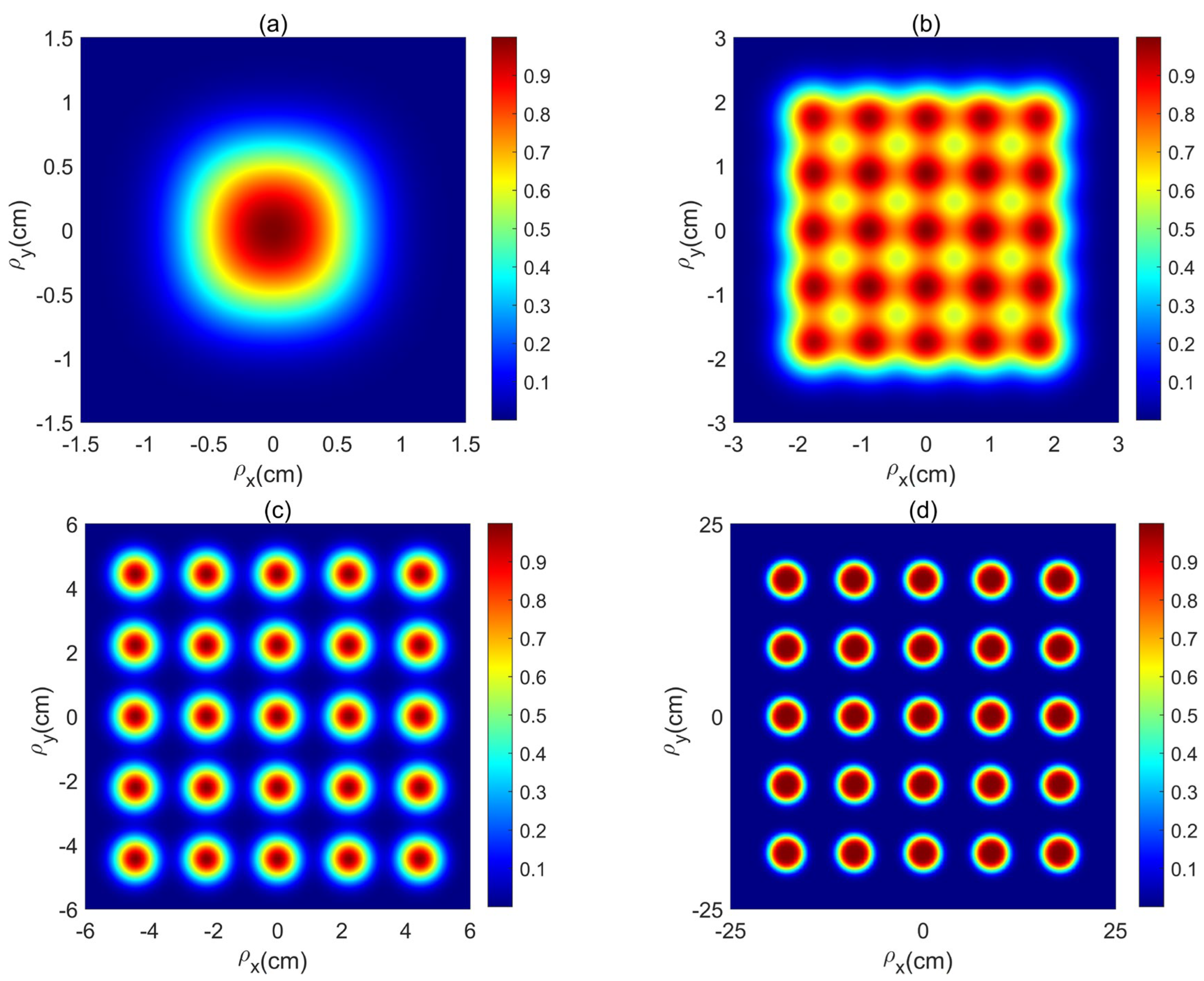
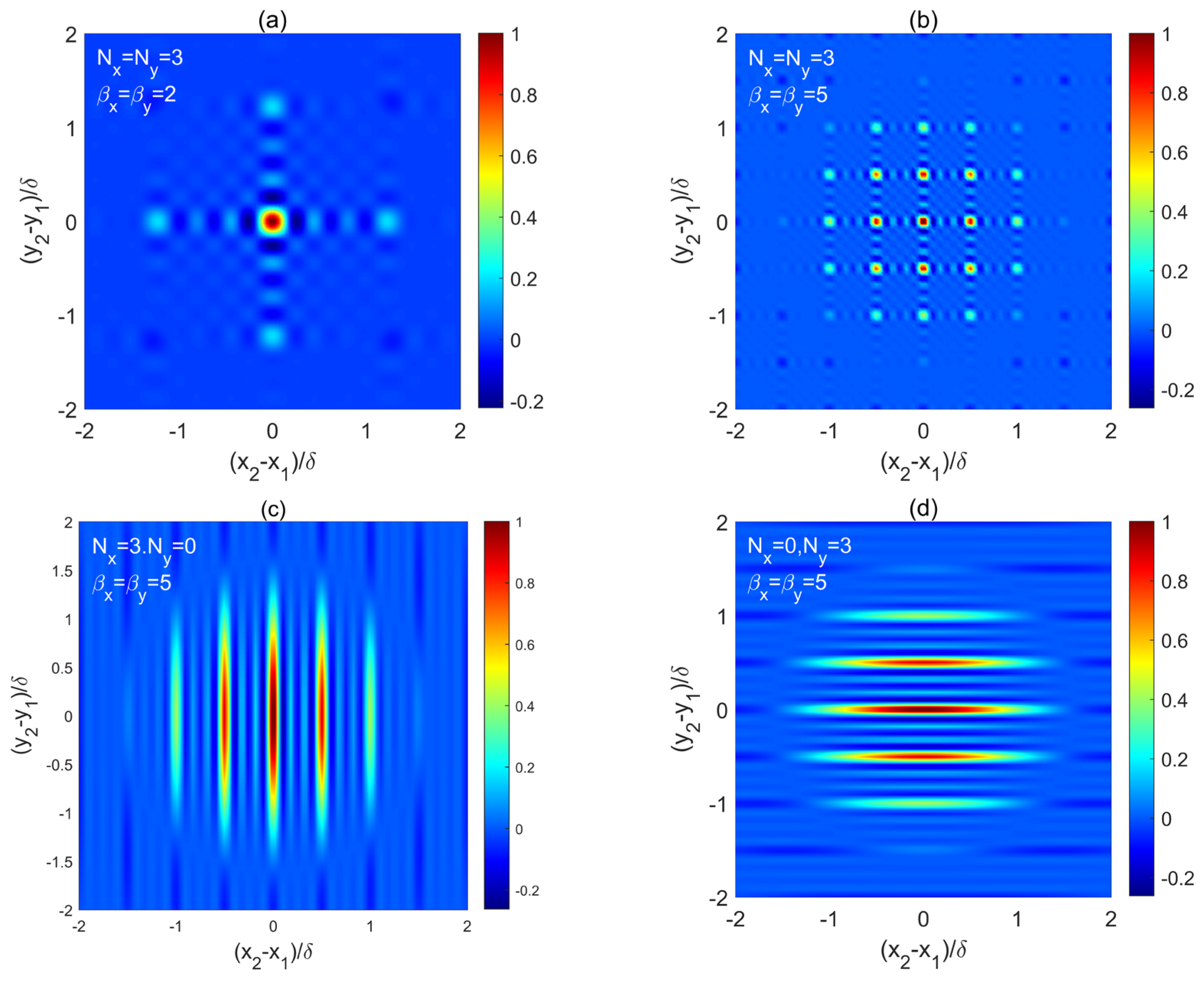
where $\mu \left({\mathbf{r}}_1,{\mathbf{r}}_2\right)$ is the degree of coherence (DOC). The newly obtained $\mu \left({\mathbf{r}}_1,{\mathbf{r}}_2\right)$ in this work is different from Equation (5) of the previous work [21]; the introduced beam which consists of a multi-cosine component and a multi-Gaussian component in this work will split into a rectangular beam array during propagation. The number of beamlets can be controlled by the multi-cosine component, and the flatness of the beamlets can be manipulated by the multi-Gaussian component. When ${\beta }_x={\beta }_y=0$ in Equation (5), the McMGCB will reduce to an MGSM beam. When $F=1$ in Equation (5), the McMGCB will reduce to a multi-cosine-multi-Gaussian correlated beam. The DOC of the McMGCB will exhibit array profiles when ${\beta }_x={\beta }_y\ne 0$ (Figure 1a,b), and the distribution of the DOC is controlled by parameters. When $N_y=0$, the DOC of McMGCB will show lines along the x-axis (Figure 1c), and the DOC of McMGCB with $N_x=0$ will show lines along the y-axis (Figure 1d).

2.2. Physical Modle of McMGCB in Turbulence

In general, the paraxial propagation of a partially coherent beam in anisotropic oceanic turbulence can be described by the extended Huygens-Fresnel integral [18,19,20,21]:

$$\begin{array}{l}W\left({\mathbf{\rho }}_1,{\mathbf{\rho }}_2,z\right)={\displaystyle \frac{k^2}{4{\pi }^2{z}^2}}{\displaystyle \iint d{\mathbf{r}}_{1}d{\mathbf{r}}_2}W\left({\mathbf{r}}_1,{\mathbf{r}}_2\right)\\ \hspace{1em}\times \exp \left[-{\displaystyle \frac{ik}{2z}}{\left({\mathbf{\rho }}_1-{\mathbf{r}}_1\right)}^2+{\displaystyle \frac{ik}{2z}}{\left({\mathbf{\rho }}_2-{\mathbf{r}}_2\right)}^2\right]〈\exp \left[\psi \left({\mathbf{r}}_1,{\mathbf{\rho }}_1\right)+{\psi }^{\ast }\left({\mathbf{r}}_2,{\mathbf{\rho }}_2\right)\right]〉\end{array}$$

(6)

where $\mathbf{\rho }=\left({\rho }_x,{\rho }_y\right)$ is the position vector at plane $z$. And the last term in Equation (6) can be written as

$$〈\exp \left[\psi \left({\mathbf{r}}_1,{\mathbf{\rho }}_1\right)+{\psi }^{\ast }\left({\mathbf{r}}_2,{\mathbf{\rho }}_2\right)\right]〉=\exp \left[-{\displaystyle \frac{{\left({\mathbf{r}}_1-{\mathbf{r}}_2\right)}^2+\left({\mathbf{r}}_1-{\mathbf{r}}_2\right)\left({\mathbf{\rho }}_1-{\mathbf{\rho }}_2\right)+{\left({\mathbf{\rho }}_1-{\mathbf{\rho }}_2\right)}^2}{{\mathrm{\Lambda }}^2}}\right]$$

(7)

The parameter in anisotropic oceanic turbulence in Equation (7) can be given as [23,24,25]

$$\mathrm{\Lambda }={\left[8.705\times {10}^{-8}{k}^{2}z{\left(\epsilon \eta \right)}^{-1/3}{\zeta }^{-2}{\chi }_T\left(1-2.605{\varpi }^{-1}+7.007{\varpi }^{-2}\right)\right]}^{-1/2}$$

(8)

where $\varsigma$ is the anisotropic factor. $\epsilon$ denotes the dissipation rate of fluid which ranging from ${10}^{-10} {\mathrm{m}}^2/{\mathrm{s}}^3$ to ${10}^{-1} {\mathrm{m}}^2/{\mathrm{s}}^3$. $\varpi$ is the ratio of temperature and salinity which can be set as $\left[-5,0\right]$. $\eta$ denotes the inner scale. ${\chi }_T$ gives the dissipation of temperature which ranging from ${10}^{-10} {\mathrm{K}}^2/\mathrm{s}$ to ${10}^{-4} {\mathrm{K}}^2/\mathrm{s}$.

Considering Equations (7) and (8), and substituting Equation (4) into Equation (6), the CSD of McMGCB in anisotropic oceanic turbulence at $z$ is derived as:

$$\begin{array}{l}W\left({\mathbf{\rho }}_1,{\mathbf{\rho }}_2,z\right)={\displaystyle \frac{k^2}{4{\pi }^2{z}^2}}{C}_0\exp \left[{\displaystyle \frac{ik}{2z}}\left({\mathbf{\rho }}_2^2-{\mathbf{\rho }}_1^2\right)\right]\exp \left[-{\displaystyle \frac{{\left({\rho }_{1x}-{\rho }_{2x}\right)}^2+{\left({\rho }_{1y}-{\rho }_{2y}\right)}^2}{{\mathrm{\Lambda }}^2}}\right]\\ {\displaystyle {\displaystyle \sum _{f=1}^F}\frac{{\left(-1\right)}^{f-1}}{f}}\left(\begin{array}{c}F\\ f\end{array}\right){\displaystyle {\displaystyle \sum _{n=-N_x}^{N_x}}}{\displaystyle {\displaystyle \sum _{m=-N_y}^{N_y}}}{\displaystyle \frac{1}{4}}\left(S_{x+}+S_{x-}\right)\left(S_{y+}+S_{y-}\right)\end{array}$$

(9)

where

$$S_{x+}={\displaystyle \frac{\pi }{\sqrt{ab}}}\exp \left({\displaystyle \frac{c_{x+}^2}{b_x}}\right)\exp \left[{\displaystyle \frac{1}{a}}{\left({\displaystyle \frac{ik}{2z}}{\rho }_{1x}-i{\displaystyle \frac{\sqrt{2\pi }n{\beta }_x}{2\delta }}-{\displaystyle \frac{{\rho }_{1x}-{\rho }_{2x}}{2{\mathrm{\Lambda }}^2}}\right)}^2\right]$$

(10)

$$S_{x-}={\displaystyle \frac{\pi }{\sqrt{ab}}}\exp \left({\displaystyle \frac{c_{x-}^2}{b}}\right)\exp \left[{\displaystyle \frac{1}{a}}{\left({\displaystyle \frac{ik}{2z}}{\rho }_{1x}+i{\displaystyle \frac{\sqrt{2\pi }n{\beta }_x}{2\delta }}-{\displaystyle \frac{{\rho }_{1x}-{\rho }_{2x}}{2{\mathrm{\Lambda }}^2}}\right)}^2\right]$$

(11)

$$S_{y+}={\displaystyle \frac{\pi }{\sqrt{ab}}}\exp \left({\displaystyle \frac{c_{y+}^2}{b}}\right)\exp \left[{\displaystyle \frac{1}{a}}{\left({\displaystyle \frac{ik}{2z}}{\rho }_{1y}-i{\displaystyle \frac{\sqrt{2\pi }m{\beta }_y}{2\delta }}-{\displaystyle \frac{{\rho }_{1y}-{\rho }_{2y}}{2{\mathrm{\Lambda }}^2}}\right)}^2\right]$$

(12)

$$S_{y-}={\displaystyle \frac{\pi }{\sqrt{ab}}}\exp \left({\displaystyle \frac{c_{y-}^2}{b}}\right)\exp \left[{\displaystyle \frac{1}{a}}{\left({\displaystyle \frac{ik}{2z}}{\rho }_{1y}+i{\displaystyle \frac{\sqrt{2\pi }m{\beta }_y}{2\delta }}-{\displaystyle \frac{{\rho }_{1y}-{\rho }_{2y}}{2{\mathrm{\Lambda }}^2}}\right)}^2\right]$$

(13)

with

$$a={\displaystyle \frac{1}{4w_0^2}}+{\displaystyle \frac{1}{2f{\delta }^2}}+{\displaystyle \frac{1}{{\mathrm{\Lambda }}^2}}+{\displaystyle \frac{ik}{2z}}$$

(14)

$$b={\displaystyle \frac{1}{4w_0^2}}+{\displaystyle \frac{1}{2f{\delta }^2}}+{\displaystyle \frac{1}{{\mathrm{\Lambda }}^2}}-{\displaystyle \frac{ik}{2z}}-{\displaystyle \frac{1}{a}}{\left({\displaystyle \frac{1}{2f{\delta }^2}}+{\displaystyle \frac{1}{{\mathrm{\Lambda }}^2}}\right)}^2$$

(15)

$$c_{x+}={\displaystyle \frac{1}{a}}\left({\displaystyle \frac{1}{2f{\delta }^2}}+{\displaystyle \frac{1}{{\mathrm{\Lambda }}^2}}\right)\left({\displaystyle \frac{ik}{2z}}{\rho }_{1x}-i{\displaystyle \frac{\sqrt{2\pi }n{\beta }_x}{2\delta }}-{\displaystyle \frac{{\rho }_{1x}-{\rho }_{2x}}{2{\mathrm{\Lambda }}^2}}\right)-{\displaystyle \frac{ik}{2z}}{\rho }_{2x}+{\displaystyle \frac{{\rho }_{1x}-{\rho }_{2x}}{2{\mathrm{\Lambda }}^2}}+i{\displaystyle \frac{\sqrt{2\pi }n{\beta }_x}{2\delta }}$$

(16)

$$c_{x-}={\displaystyle \frac{1}{a}}\left({\displaystyle \frac{1}{2f{\delta }^2}}+{\displaystyle \frac{1}{{\mathrm{\Lambda }}^2}}\right)\left({\displaystyle \frac{ik}{2z}}{\rho }_{1x}+i{\displaystyle \frac{\sqrt{2\pi }n{\beta }_x}{2\delta }}-{\displaystyle \frac{{\rho }_{1x}-{\rho }_{2x}}{2{\mathrm{\Lambda }}^2}}\right)-{\displaystyle \frac{ik}{2z}}{\rho }_{2x}+{\displaystyle \frac{{\rho }_{1x}-{\rho }_{2x}}{2{\mathrm{\Lambda }}^2}}-i{\displaystyle \frac{\sqrt{2\pi }n{\beta }_x}{2\delta }}$$

(17)

$$c_{y+}={\displaystyle \frac{1}{a}}\left({\displaystyle \frac{1}{2f{\delta }^2}}+{\displaystyle \frac{1}{{\mathrm{\Lambda }}^2}}\right)\left({\displaystyle \frac{ik}{2z}}{\rho }_{1y}-i{\displaystyle \frac{\sqrt{2\pi }m{\beta }_y}{2\delta }}-{\displaystyle \frac{{\rho }_{1y}-{\rho }_{2y}}{2{\mathrm{\Lambda }}^2}}\right)-{\displaystyle \frac{ik}{2z}}{\rho }_{2y}+{\displaystyle \frac{{\rho }_{1y}-{\rho }_{2y}}{2{\mathrm{\Lambda }}^2}}+i{\displaystyle \frac{\sqrt{2\pi }m{\beta }_y}{2\delta }}$$

(18)

$$c_{y-}={\displaystyle \frac{1}{a}}\left({\displaystyle \frac{1}{2f{\delta }^2}}+{\displaystyle \frac{1}{{\mathrm{\Lambda }}^2}}\right)\left({\displaystyle \frac{ik}{2z}}{\rho }_{1y}+i{\displaystyle \frac{\sqrt{2\pi }m{\beta }_y}{2\delta }}-{\displaystyle \frac{{\rho }_{1y}-{\rho }_{2y}}{2{\mathrm{\Lambda }}^2}}\right)-{\displaystyle \frac{ik}{2z}}{\rho }_{2y}+{\displaystyle \frac{{\rho }_{1y}-{\rho }_{2y}}{2{\mathrm{\Lambda }}^2}}-i{\displaystyle \frac{\sqrt{2\pi }m{\beta }_y}{2\delta }}$$

(19)

In the derivation of Equations (9)–(19), the following equation has been used:

$${\displaystyle {\int }_{-\infty }^{+\infty }\exp \left(-p{x}^2+2qx\right)dx}=\sqrt{{\displaystyle \frac{\pi }{p}}}\exp \left({\displaystyle \frac{q^2}{p}}\right)$$

(20)

Equations (9)–(19) are the main results of this work, the properties of such McMGCB can be analyzed based on the above derived equations. When $\mathbf{\rho }={\mathbf{\rho }}_1={\mathbf{\rho }}_2$ in Equations (9)–(19), the intensity of McMGCB at $z$ can be given by [26]

$$I\left(\mathbf{\rho },z\right)=W\left(\mathbf{\rho },\mathbf{\rho },z\right)$$

(21)

The degree of coherence of McMGCB at $z$ can be given by [26]

$$\mu \left({\mathbf{\rho }}_1,{\mathbf{\rho }}_2,z\right)={\displaystyle \frac{W\left({\mathbf{\rho }}_1,{\mathbf{\rho }}_2,z\right)}{\sqrt{W\left({\mathbf{\rho }}_1,{\mathbf{\rho }}_1,z\right)W\left({\mathbf{\rho }}_2,{\mathbf{\rho }}_2,z\right)}}}$$

(22)

3. Numerical Calculation and Analysis

This section illustrates the propagation properties of McMGCB, and focuses on the intensity and coherence properties of such McMGCB in free space and turbulence. Unless specified explanations, the parameters are set as: $\lambda =417 \mathrm{nm}$, $w_0=3 \mathrm{mm}$, $\delta =1.5 \mathrm{mm}$, $F=15$, $N_x=N_y=2$, and ${\beta }_x={\beta }_y=4$, $x_T=1\ast {10}^{-7} {\mathrm{K}}^2/\mathrm{s}$, $\varsigma =2$, $\varpi =-2$, $\epsilon =1\times {10}^{-7}{\mathrm{m}}^{-3}/{\mathrm{s}}^2$, and $\eta =1 \mathrm{mm}$.

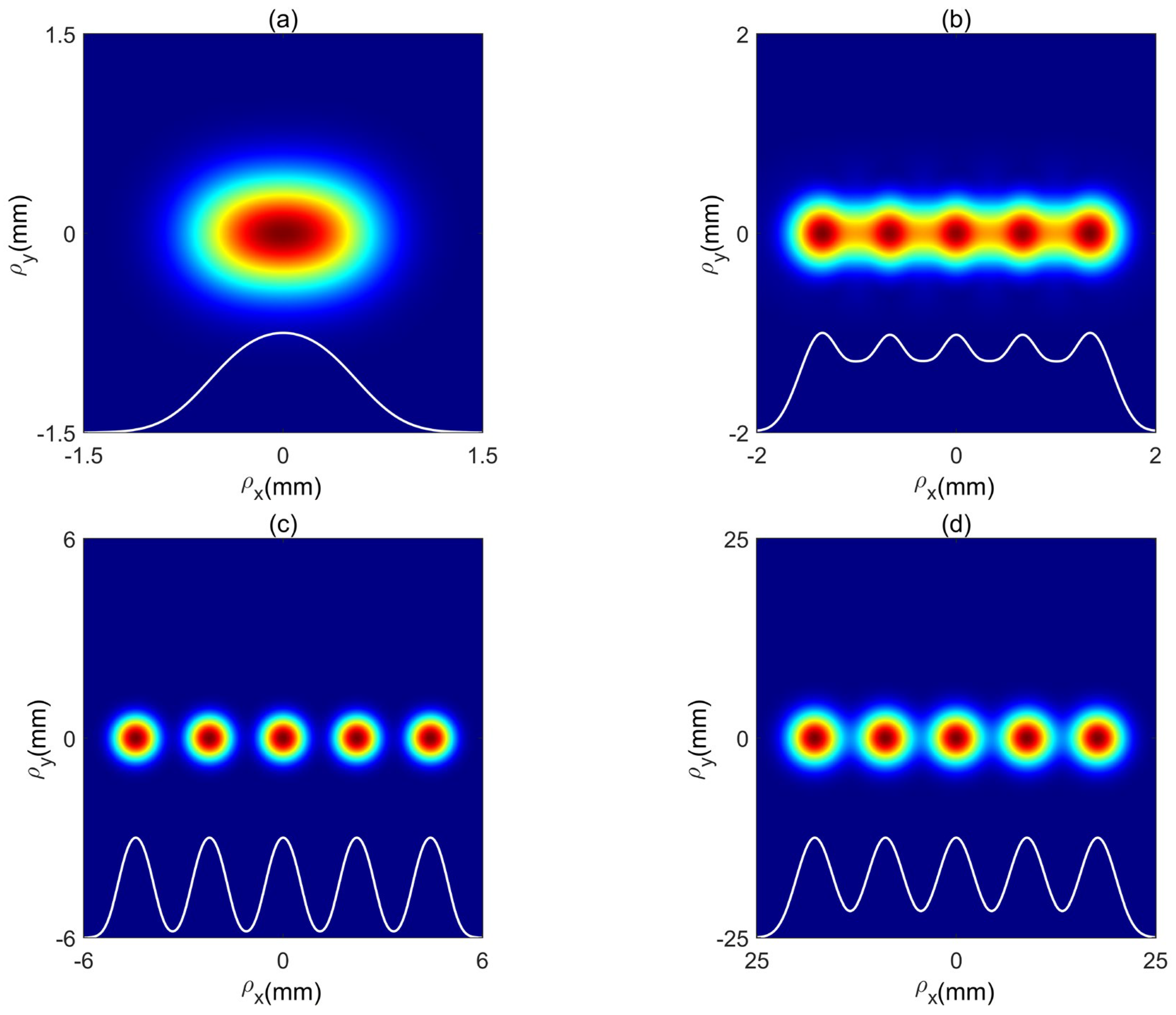
First, the normalized intensity of an McMGCB in free space is shown in Figure 2. The one spot pattern of such an McMGCB will be retained at short distance $z=5 \mathrm{m}$ (Figure 2a). As $z$ increases, the intensity of such McMGCB will gradually split (Figure 2b), and the intensity profile can evolve into an array profile composed of Gaussian beamlets (Figure 2c). At the larger distance $z=200 \mathrm{m}$, the intensity profile of such McMGCB can evolve into beam array composed of $\left(2N_x+1\right)\times \left(2N_y+1\right)$ flat-topped beamlets. (Figure 2d).

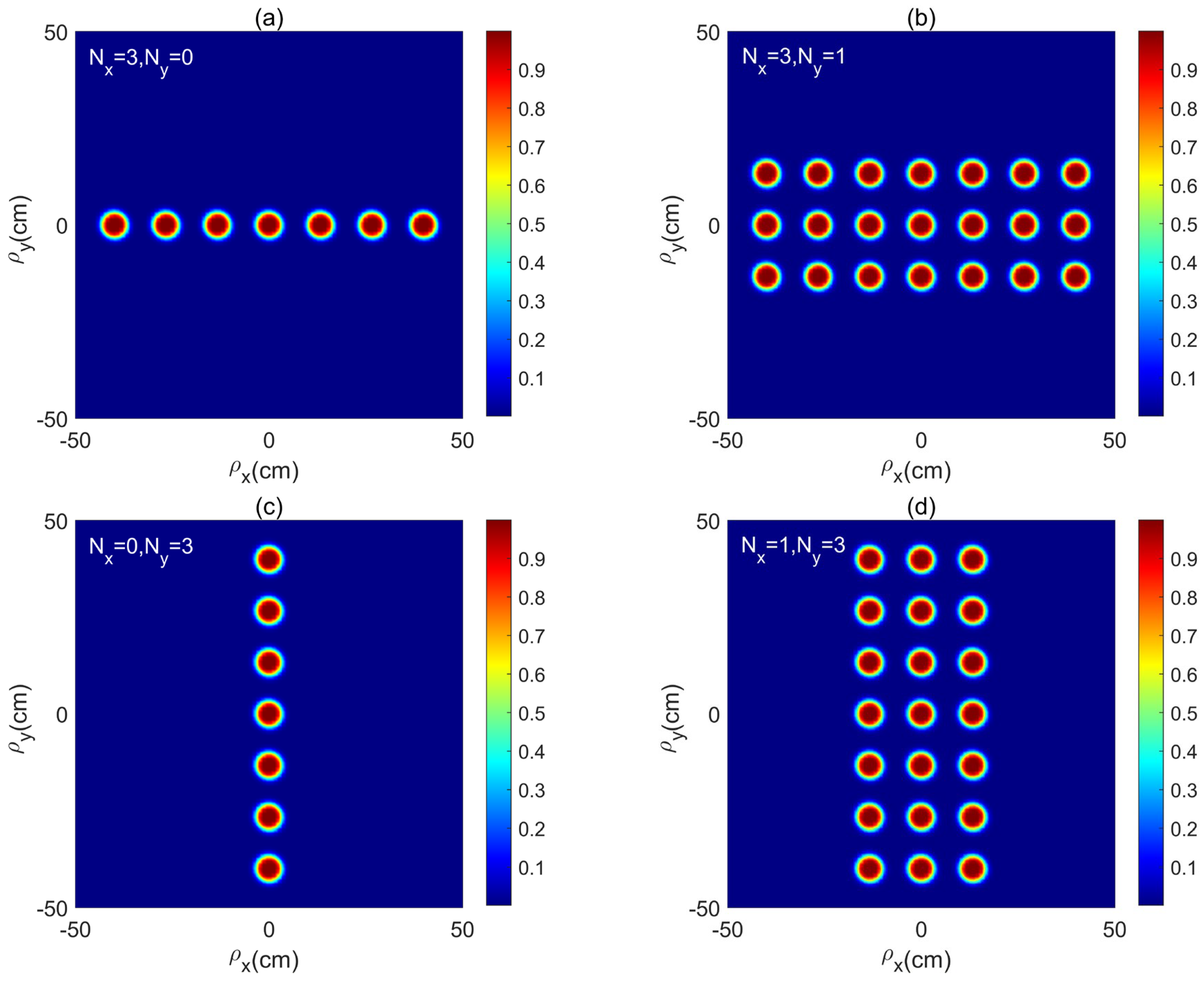
To see the relationship between intensity and parameters $N_x$ and $N_y$, Figure 3 illustrates the normalized intensity profiles of McMGCB for the different $N_x$ and $N_y$ in free space at $z=200 \mathrm{m}$. When $N_y=0$, the intensity of McMGCB with $N_x=3$ can become a line array composed of seven ($2N_x+1$) flat-topped beamlets along the x-axis (Figure 3a). As $N_y$ increases, the number of lines along y-axis will increase, and the intensity of McMGCB can evolve into a rectangular array composed of $\left(2N_x+1\right)\times \left(2N_y+1\right)$ flat-topped beamlets (Figure 3b). In contrast, the intensity of McMGCB with $N_x=0$ will become a line array composed of $2N_y+1$ flat-topped beamlets along the y-axis (Figure 3c). And as $N_x$ increases, the number of lines of array along y-axis will increase, and the McMGCB will evolve into a rectangular flat-topped array (Figure 3d). Therefore, the lines of a flat-topped beam array can be controlled by the setting $N_x$ and $N_y$, and the intensity array will have $\left(2N_x+1\right)\times \left(2N_y+1\right)$ flat-topped beamlets.

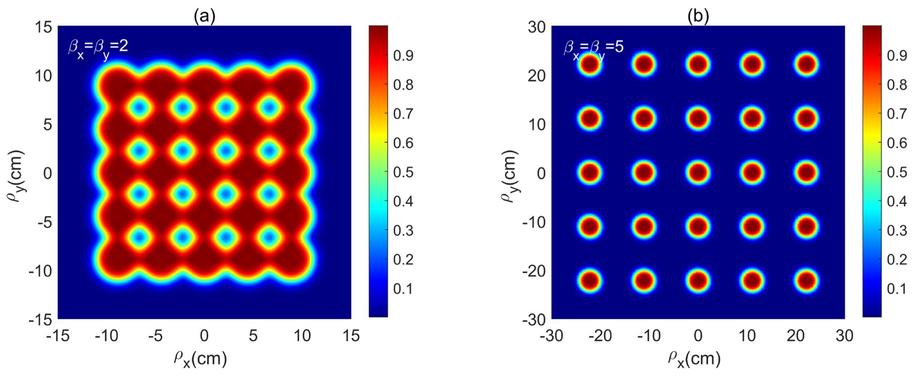
Figure 4 shows the intensity of McMGCB for the different ${\beta }_x$ and ${\beta }_y$ in free space at $z=200 \mathrm{m}$. When ${\beta }_x={\beta }_y=2$, the splitting phenomenon of such an McMGCB is found, but the beamlets coincide with each other. And when ${\beta }_x={\beta }_y$ increases to ${\beta }_x={\beta }_y=5$, the McMGCB will split into a flat-topped beam array (Figure 4b). Thus, the splitting beamlets are modulated by ${\beta }_x$ and ${\beta }_y$, and the splitting phenomenon of the McMGCB with a larger ${\beta }_x={\beta }_y$ is easily observed during propagation.

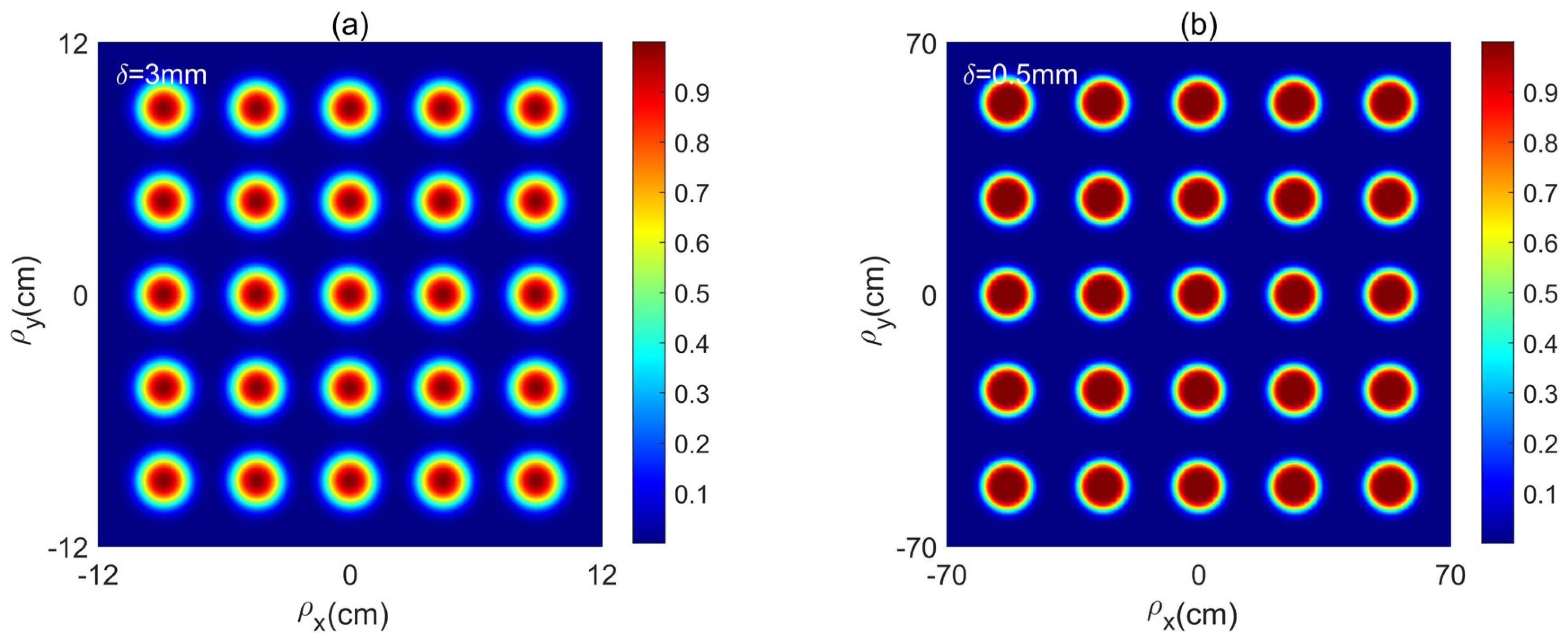
The intensity profiles of McMGCB for the different $\delta$ in free space at $z=200 \mathrm{m}$ are illustrated in Figure 5. When $\delta =3 \mathrm{mm}$, the intensity pattern of McMGCB with larger $\delta$ will split slower and just split into a beam array composed of Gaussian beamlets (Figure 5a). When $\delta$ decreases to $\delta =0.5 \mathrm{mm}$, the intensity profiles of McMGCB with smaller $\delta$ will split into an array composed of flat-topped beamlets (Figure 5b). So, the smaller $\delta$ is beneficial to the flat-topped beam array.

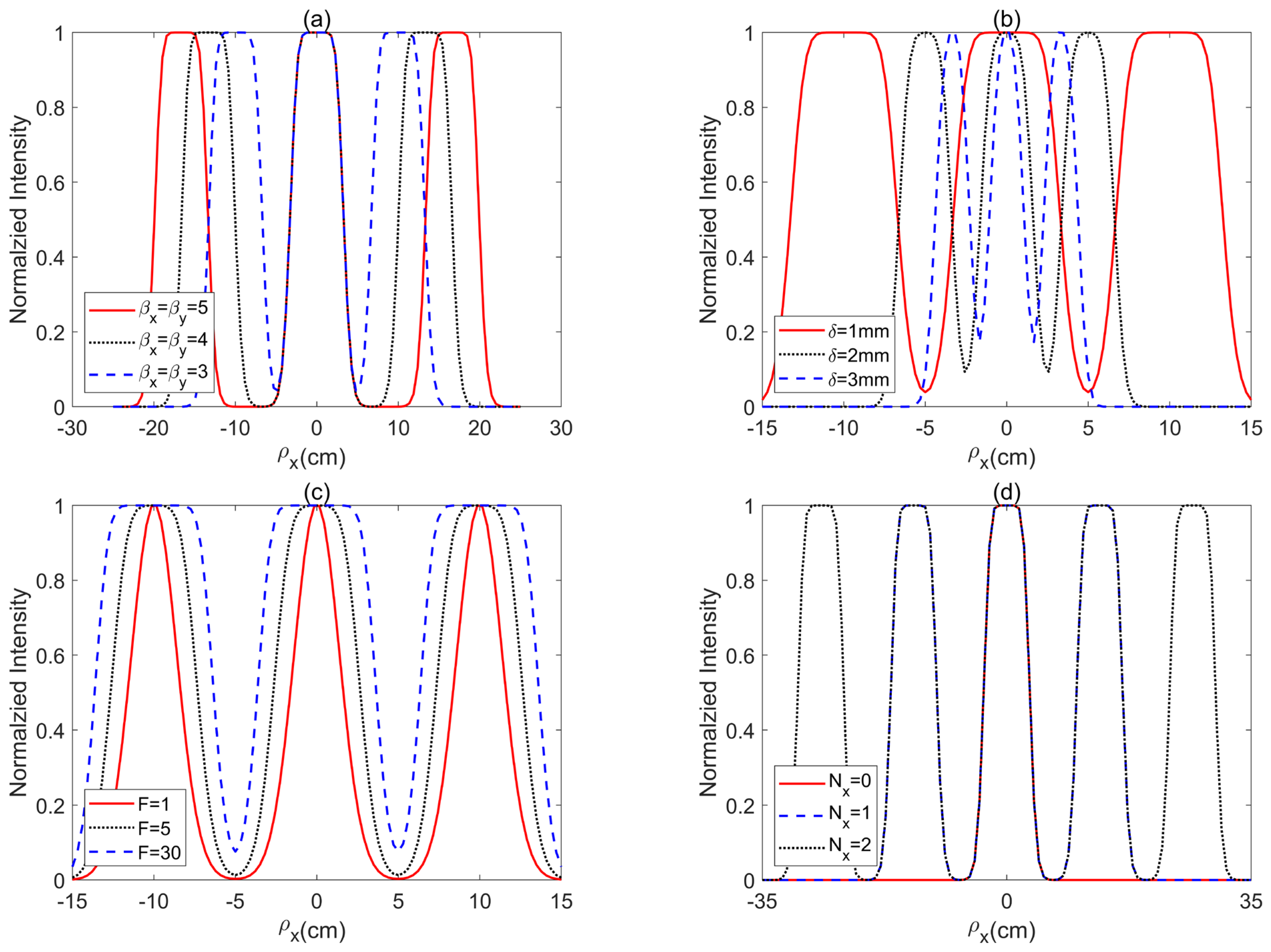
To study the influences of beam parameter on the evolution of McMGCB, the cross-sections of McMGCB with $N_x=0$ and $N_y=0$ in free space at $z=200 \mathrm{m}$ is shown in Figure 6. When ${\beta }_x$ is modulated, the distance of beamlets can increase as the ${\beta }_x$ increases (Figure 6a), and the result is consistent with the results of Figure 4. Figure 6b shows the intensity of McMGCB for the different $\delta$; the splitting phenomenon of the McMGCB will become evident as $\delta$ decreases, and the flatness of the beamlets of McMGCB with smaller $\delta$ will improve (Figure 6b), which is a similar phenomenon observed in previous Figure 5. As $F$ increases, the flatness of beamlets of McMGCB with $\delta =1 \mathrm{mm}$ will improve (Figure 6c); thus, the larger $F$ is beneficial to flatness of beamlet. When $N_x$ increases, the number of beamlets of McMGCB will increase and become an array composed of $2N_x+1$ beamlets (Figure 6d).

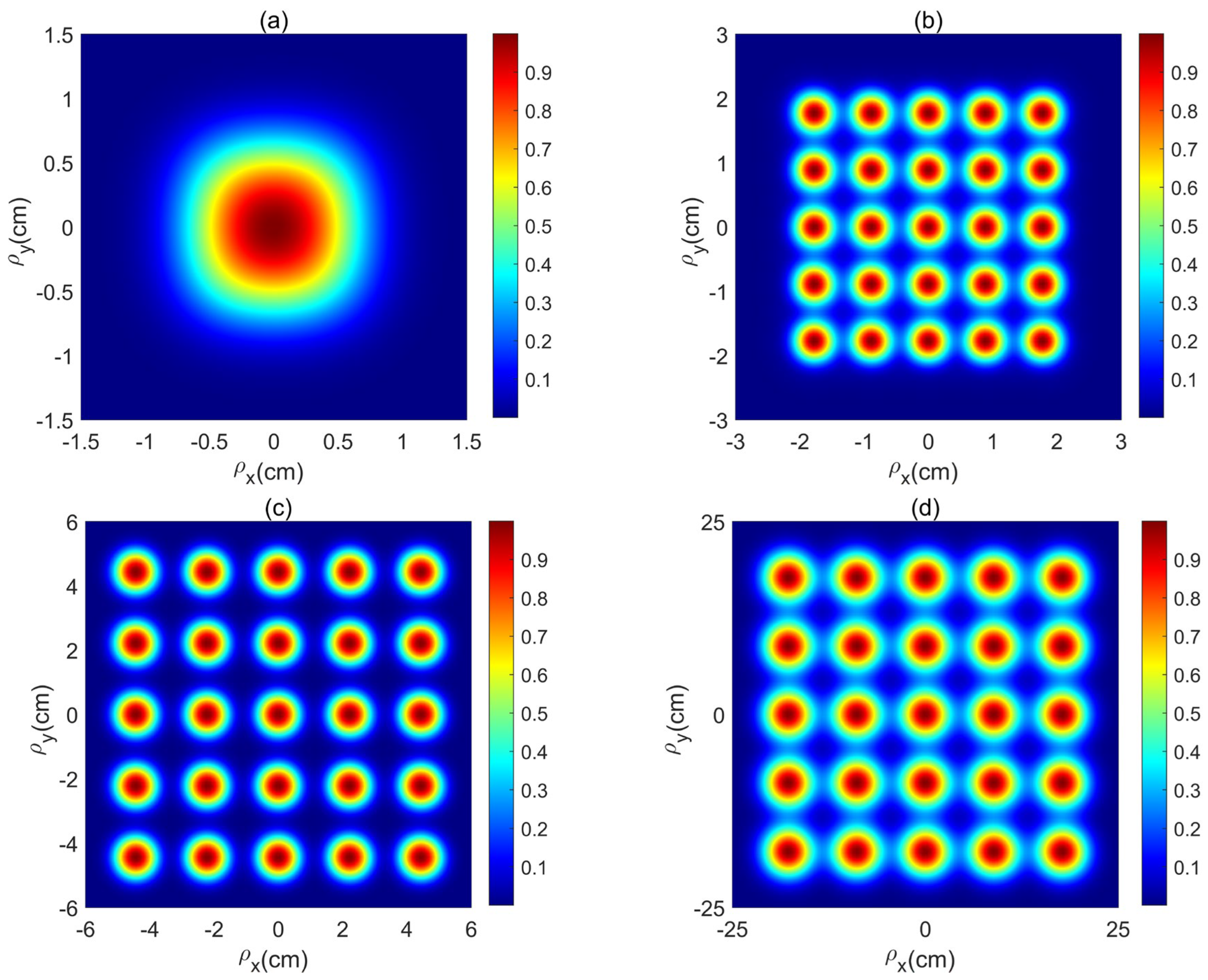
Next, the propagation of McMGCB in anisotropic oceanic turbulence is investigated. At a short distance of $z=5 \mathrm{m}$, the one spot pattern will be retained (Figure 7a). And the intensity profile of McMGCB in anisotropic oceanic turbulence can also evolve from one spot to an array profile as it increases (Figure 7b,c). At a longer distance of $z=200 \mathrm{m}$, the intensity of the McMGCB in anisotropic oceanic turbulence will show an array profile composed of Gaussian beamlets, and the overlapping phenomenon of beamlets can be seen (Figure 7d). In contrast, the intensity profile of the same McMGCB in free space will become an array composed of flat-topped beamlets (Figure 2d). Thus, the flat-topped profiles of the beamlets will be destroyed by the turbulence.

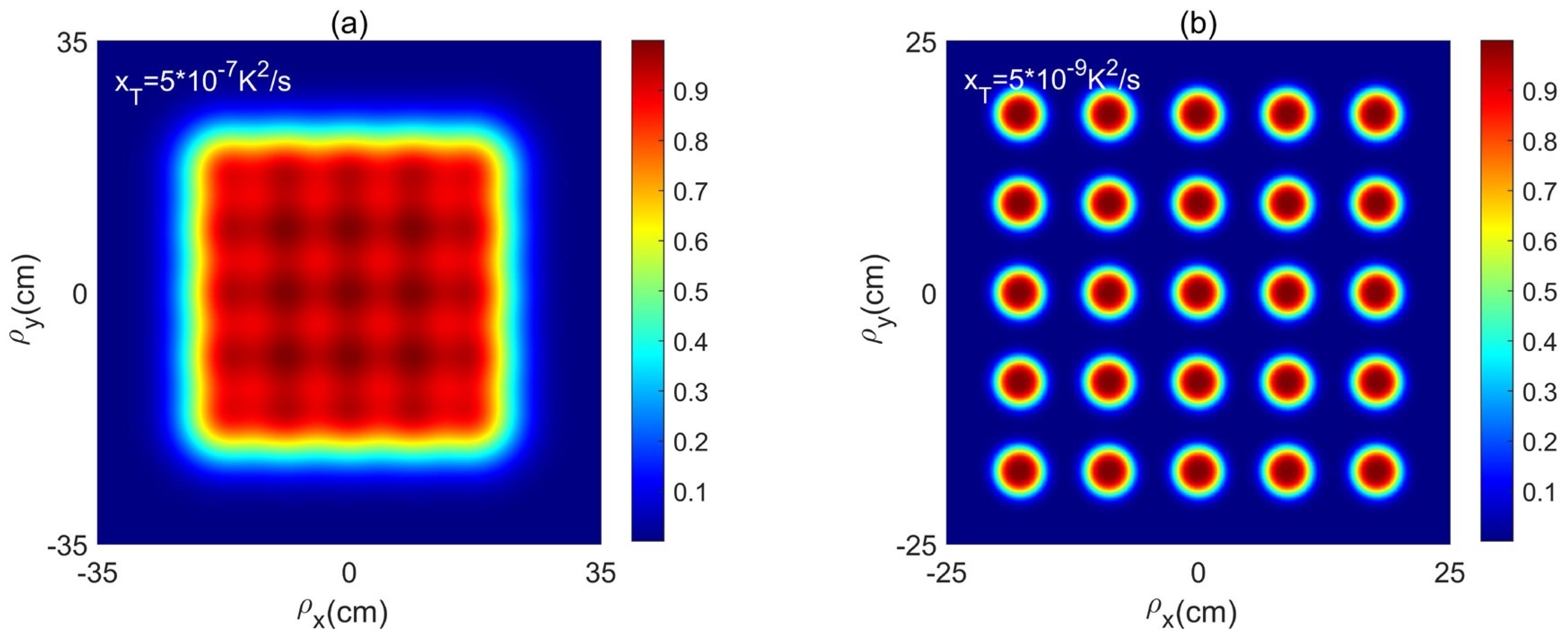
Figure 8 shows the evolution of the McMGCB in oceanic turbulence for the different $x_T$ at $z=200 \mathrm{m}$. When $x_T$ is set to a larger value where $x_T=5\ast {10}^{-7} {\mathrm{K}}^2/\mathrm{s}$, the array profiles of McMGCB will be lost and the beamlets will evolve into one spot (Figure 8a). When $x_T$ decreases, the McMGCB in oceanic turbulence with a smaller $x_T$ can retain its array profiles composed of flat-topped beamlets (Figure 8b), but the flatness of beamlets of McMGCB in free space will have better flatness.

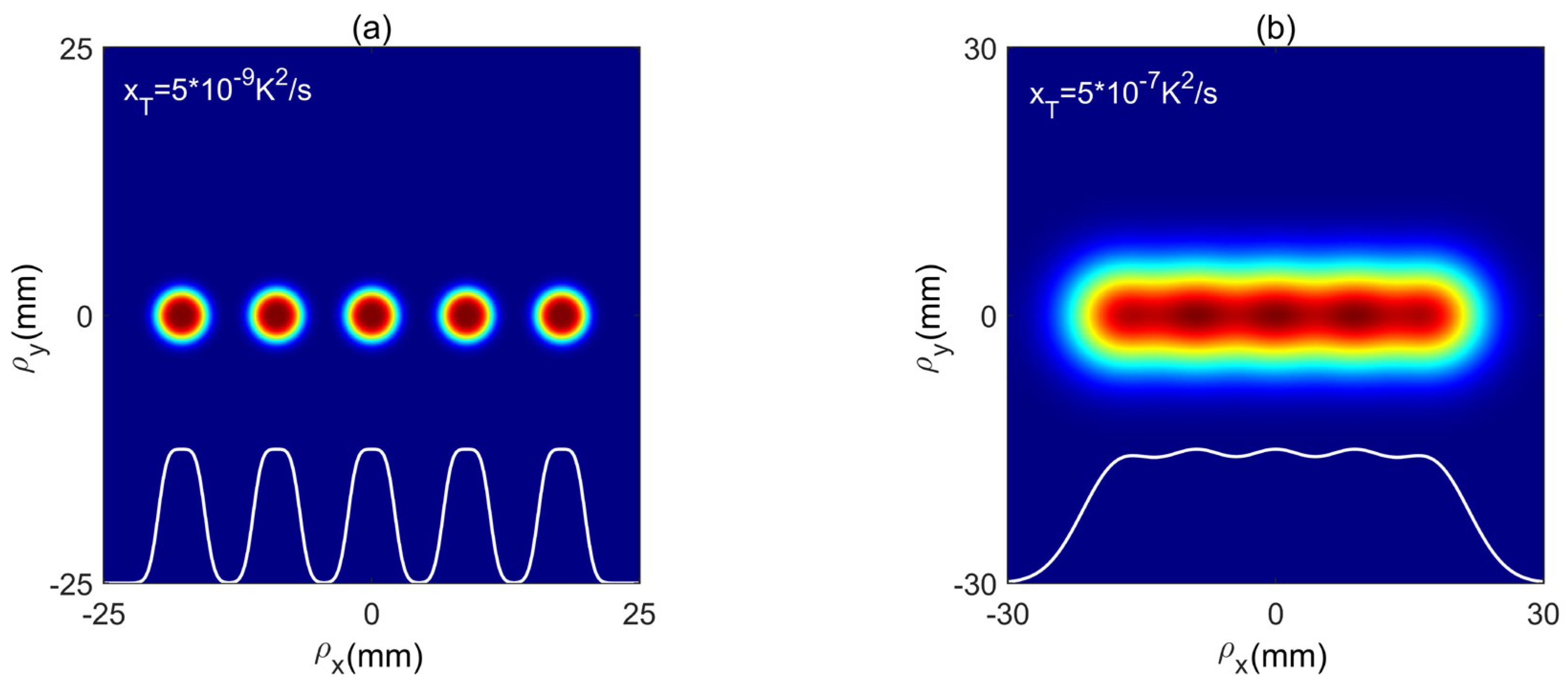
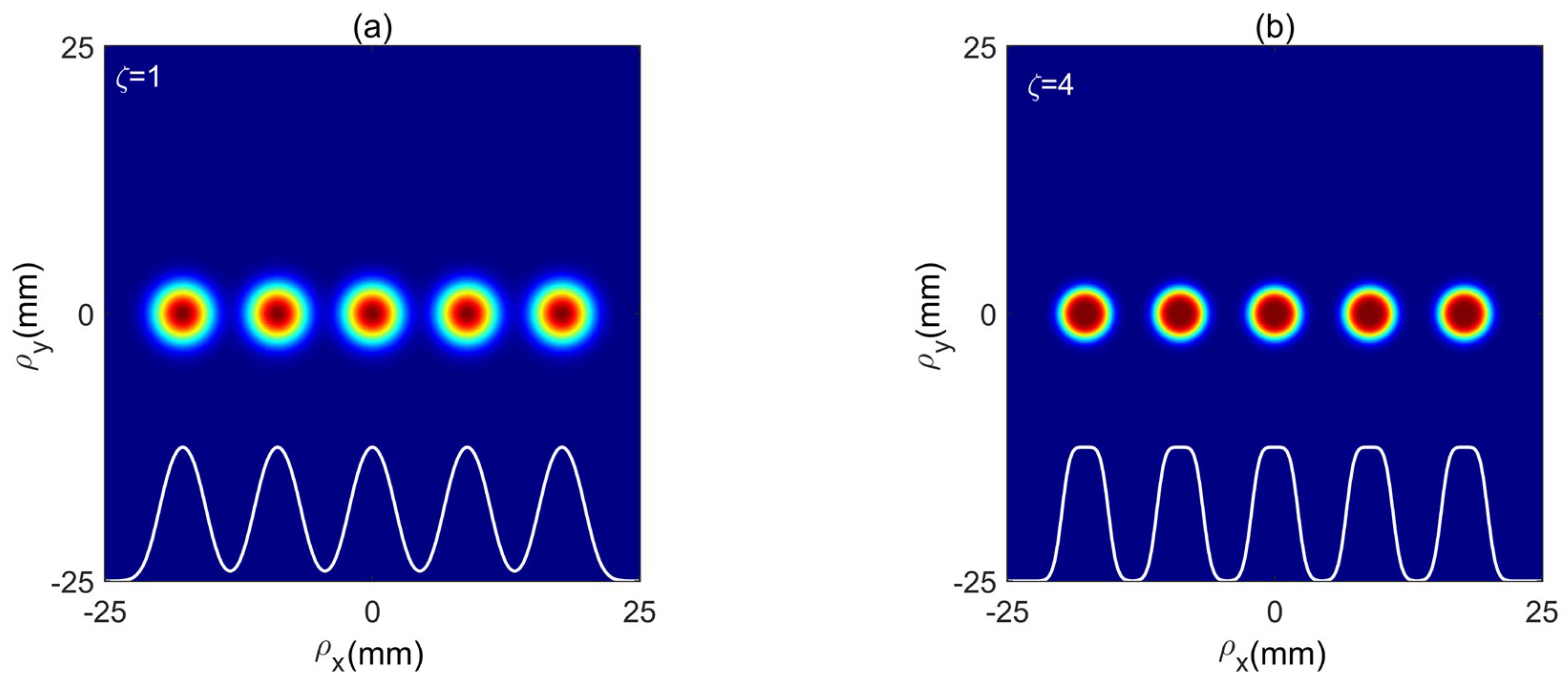
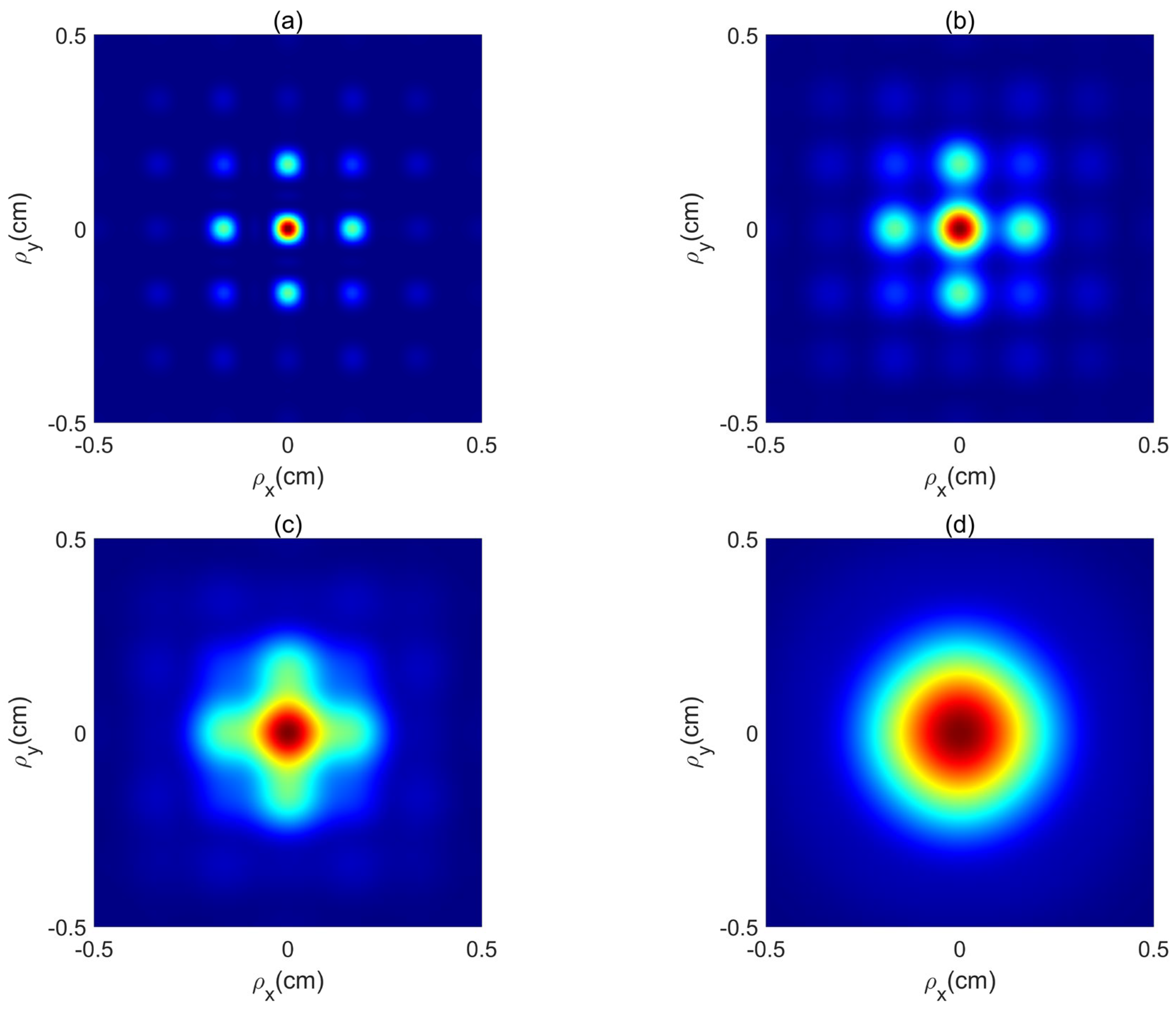
To view the effect of the turbulence on the McMGCB, the profiles of the McMGCB with $N_x=2$ and $N_y=0$ in anisotropic oceanic turbulence are given in Figure 9, Figure 10 and Figure 11. At $z=5 \mathrm{m}$, the profile of such McMGCB can have a spot profile (Figure 9a). As $z$ increases, the McMGCB can exhibit the splitting phenomenon (Figure 9b), and split into a linear array composed of $2N_x+1$ beamlets (Figure 9c). At $z=200 \mathrm{m}$, this McMGCB will still retain a linear array profile, but the overlapping phenomenon has been seen (Figure 9d). But, the McMGCB with $N_y=0$ in free space will show a linear array composed of flat-topped beamlets (Figure 3a). When the strength of turbulence is weak, this McMGCB in oceanic turbulence with smaller $x_T=5\ast {10}^{-9} {\mathrm{K}}^2/\mathrm{s}$ at $z=200 \mathrm{m}$ will retain a linear beam array composed of flat-topped beamlets (Figure 10a). But, the beamlets of the same McMGCB in oceanic turbulence with larger $x_T=5\ast {10}^{-7} {\mathrm{K}}^2/\mathrm{s}$ will overlap and translate into one spot (Figure 10b). When $\varsigma$ changes, the intensity of this McMGCB with $N_x=2$ and $N_y=0$ in oceanic turbulence with a smaller $\varsigma =1$ at $z=200 \mathrm{m}$ will become a linear array composed of a Gaussian profile (Figure 11a). In contrast, the same McMGCB in oceanic turbulence with a larger $\varsigma =4$ will retain a linear beam array composed of flat-topped beamlets (Figure 11b). Thus, the array profile composed of flat-topped beamlets can be realized when the beam in weak turbulence, and the strong turbulence will destroy the array profile.

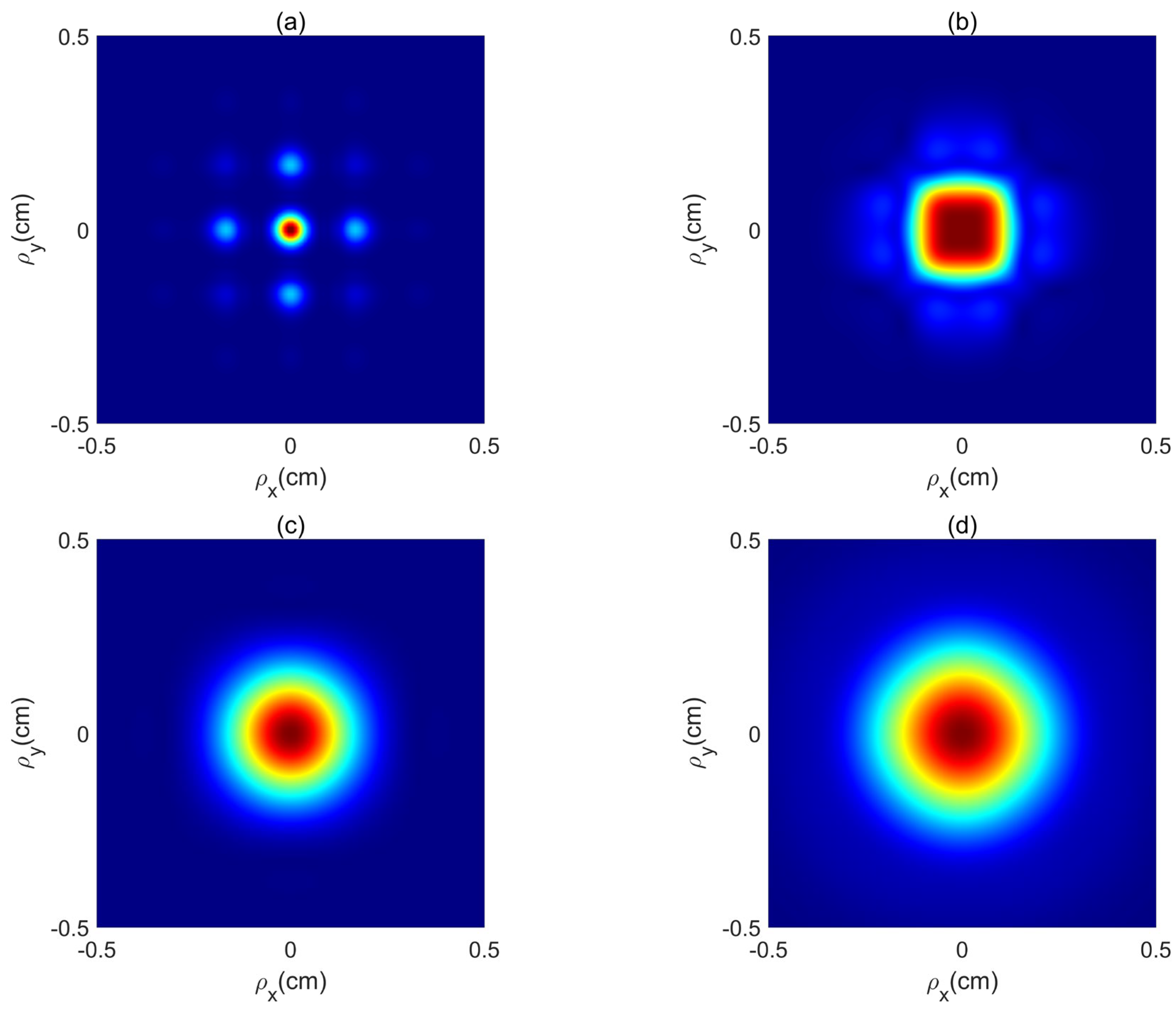
Figure 12 shows the DOC $\left|\mu \left({\mathbf{\rho }}_1-{\mathbf{\rho }}_2\right)\right|$ of an McMGCB in free space. At a short distance, the array profiles of $\left|\mu \left({\mathbf{\rho }}_1-{\mathbf{\rho }}_2\right)\right|$ of an McMGCB can be retained (Figure 12a,b). As $z$ increases, the DOC of this McMGCB will become one spot pattern (Figure 12c,d). When this McMGCB propagates in oceanic turbulence, the profiles of the DOC $\left|\mu \left({\mathbf{\rho }}_1-{\mathbf{\rho }}_2\right)\right|$ of McMGCB can retain the array profile at short distance (Figure 13a). And as $z$ increases further, the $\left|\mu \left({\mathbf{\rho }}_1-{\mathbf{\rho }}_2\right)\right|$ of such McMGCB will become one spot quickly (Figure 13b–d). From Figure 12 and Figure 13, one sees that the coherence pattern of McMGCB in turbulence will become Gaussian-like faster as $z$ increases.

4. Conclusions

In this work, the model of a flat-topped lattice named McMGCB has been introduced, the coherence function of an McMGCB consists of a multi-cosine component and a multi-Gaussian coment, and the CSD of such an McMGCB in anisotropic oceanic turbulence has been derived. The splitting properties of the McMGCB are caused by multi-cosine part of coherence function, and the flatness of beamlets will be controlled by the multi-Gaussian part of the coherence function. The intensity of such an McMGCB in free space can evolve into a rectangular flat-topped beam array; the flatness of the beamlets can be controlled by $F$ and $\delta$, and the number of rectangular lines of array are controlled by parameters $N_x$ and $N_y$. However, the flat-topped beam array profiles of such an McMGCB in oceanic turbulence can be destroyed by the turbulence; the McMGCB in weak oceanic turbulence can translate into an array composed of Gaussian beamlets, but the beamlets of McMGCB in stronger oceanic turbulence can overlap and evolve into one spot. Therefore, the obtained characterizations of this flat-topped lattice with its adjustable parameters provide a method to generate a rectangular flat-topped beam array, and may have applications involving flat-topped beam arrays.

References

1. Cai, Y. Propagation of various flat-topped beams in a turbulent atmosphere. J. Opt. A Pure Appl. Opt. 2006, 8, 537–545. [Google Scholar] [CrossRef] [Scilit]
2. Eyyuboğlu, H.T.; Çil, C.Z. Beam wander of dark hollow, flat-topped and annular beams. Appl. Phys. B 2008, 93, 595–604. [Google Scholar] [CrossRef] [Scilit]
3. Zhang, M.; Liu, X.; Guo, L.; Liu, L.; Cai, Y. Partially Coherent Flat-Topped Beam Generated by an Axicon. Appl. Sci. 2019, 9, 1499. [Google Scholar] [CrossRef] [Scilit]
4. Wang, X.; Zhang, H.; Gao, Y.; Wei, D.; Cai, Y.; Yuan, Y. Distribution of intensity and M2 factor for a partially coherent flat-topped beam in bidirectional turbulent atmosphere and plasma connection. Opt. Express 2024, 32, 5982. [Google Scholar] [CrossRef] [Scilit] [PubMed]
5. Sahin, S.; Korotkova, O. Light sources generating far fields with tunable flat profiles. Opt. Lett. 2012, 37, 2970–2972. [Google Scholar] [CrossRef] [Scilit] [PubMed]
6. Korotkova, O.; Sahin, S.; Shchepakina, E. Multi-Gaussian Schell-model beams. J. Opt. Soc. Am. A 2012, 29, 2159–2164. [Google Scholar] [CrossRef] [Scilit] [PubMed]
7. Korotkova, O.; Shchepakina, E. Rectangular Multi-Gaussian Schell-Model beams in atmospheric turbulence. J. Opt. 2014, 16, 045704. [Google Scholar] [CrossRef] [Scilit]
8. Wang, H.; Peng, X.; Liu, L.; Wang, F.; Cai, Y. Twisted elliptical multi-Gaussian Schell-model beams and their propagation properties. J. Opt. Soc. Am. A Opt. Image Sci. Vis. 2020, 37, 89–97. [Google Scholar] [CrossRef] [Scilit] [PubMed]
9. Zhang, Y.T.; Liu, L.; Zhao, C.L.; Cai, Y.J. Multi-Gaussian Schell-model vortex beam. Phys. Lett. A 2014, 378, 750–754. [Google Scholar] [CrossRef] [Scilit]
10. Zhang, Y.T.; Ding, C.L.; Pan, L.Z.; Cai, Y.J. Laser arrays of partially coherent beams with multi-Gaussian correlation function. J. Quant. Spectrosc. Radiat. Transf. 2018, 218, 1–11. [Google Scholar] [CrossRef] [Scilit]
11. He, L.; Zhang, N.; Yu, H.; Ji, X. Propagation dynamics of multi-Gaussian Schell model beams in strongly nonlocal nonlinear media. J. Opt. Soc. Am. A 2024, 41, 1893–1898. [Google Scholar] [CrossRef] [Scilit]
12. Zhang, Y.; Wang, J.; Qian, X.; Zhu, W.; Li, J. Orbital angular momentum evolution of twisted multi-Gaussian Schell model beams in anisotropic turbulence. Opt. Commun. 2022, 520, 128454. [Google Scholar] [CrossRef] [Scilit]
13. Feng, Y.; Xing, Y.; Liu, Y.; Wang, T.; Wu, H. Incident power-dependent spectral density analysis for multi-Gaussian Schell-model beams scattered by particle collections. Opt. Express 2025, 33, 17824. [Google Scholar] [CrossRef] [Scilit] [PubMed]
14. Ma, L.; Ponomarenko, S.A. Optical coherence gratings and lattices. Opt. Lett. 2014, 39, 6656–6659. [Google Scholar] [CrossRef] [Scilit] [PubMed]
15. Liu, X.; Yu, J.; Cai, Y.; Ponomarenko, S.A. Propagation of optical coherence lattices in the turbulent atmosphere. Opt. Lett. 2016, 41, 4182–4185. [Google Scholar] [CrossRef] [Scilit] [PubMed]
16. Liang, C.; Liu, X.; Xu, Z.; Wang, F.; Wen, W.; Ponomarenko, S.A.; Cai, Y.; Ma, P. Perfect optical coherence lattices. Appl. Phys. Lett. 2021, 119, 131109. [Google Scholar] [CrossRef] [Scilit]
17. Zhu, L.; Tang, M.; Li, H.; Tai, Y.; Li, X. Optical vortex lattice: An exploitation of orbital angular momentum. Nanophotonics 2021, 10, 2487–2496. [Google Scholar] [CrossRef] [Scilit]
18. Xu, J.; Pan, K.; Zhao, D. Random sources generating hollow array beams. Opt. Express 2020, 28, 16772–16781. [Google Scholar] [CrossRef] [Scilit] [PubMed]
19. Zhu, P.; Liu, D.; Yin, Y.; Zhong, H.; Wang, Y.; Wang, G. Effects of oceanic turbulence on a multi-cosine-Lorentz correlated beam. J. Quant. Spectrosc. Radiat. Transf. 2025, 333, 109313. [Google Scholar] [CrossRef] [Scilit]
20. Yang, X.Y.; Fu, W.Y. Propagation of radially polarized beams with a Hermite non-uniformly correlated array in free space and turbulent atmosphere. Opt. Express 2023, 31, 14403–14413. [Google Scholar] [CrossRef] [Scilit] [PubMed]
21. Cong, R.; Liu, D.; Yin, Y.; Wang, G.; Wang, Y.; Zhong, H. Cosine-multi-Gaussian correlated beam and its propagation properties in free space and oceanic turbulence. Phys. Scr. 2026, 101, 175503. [Google Scholar] [CrossRef] [Scilit]
22. Gori, F.; Santarsiero, M. Devising genuine spatial correlation functions. Opt. Lett. 2007, 32, 3531–3533. [Google Scholar] [CrossRef] [Scilit] [PubMed]
23. Chen, M.Y.; Zhang, Y.X. Effects of anisotropic oceanic turbulence on the propagation of the OAM mode of a partially coherent modified Bessel correlated vortex beam. Waves Random Complex Media 2019, 29, 694–705. [Google Scholar] [CrossRef] [Scilit]
24. Chen, L.; Liu, D.; Gao, H.; Dong, A.; Wang, Y. Research on characteristics of partially coherent radially polarized off-axis double vortex beam in oceanic turbulence. Opt. Laser Technol. 2025, 190, 113264. [Google Scholar] [CrossRef] [Scilit]
25. Cong, R.; Liu, D.; Yin, Y.; Zhong, H.; Wang, Y.; Wang, G. Research on Characteristics of the Hermite–Gaussian Correlated Vortex Beam. J. Mar. Sci. Eng. 2025, 13, 814. [Google Scholar] [CrossRef] [Scilit]
26. Wolf, E. Unified theory of coherence and polarization of random electromagnetic beams. Phys. Lett. A 2003, 312, 263–267. [Google Scholar] [CrossRef] [Scilit]
Figure 1. The DOC for a McMGCB source with (a) N x = N y = 3 and β x = β y = 2 , (b) N x = N y = 3 and β x = β y = 5 , (c) N x = 3 , N y = 0 and β x = β y = 5 , and (d) N x = 0 , N y = 3 and β x = β y = 5 .
Jmse 14 01636 g001
Figure 2. The intensity of McMGCB in free space. (a) z = 5   m , (b) z = 20   m , (c) z = 50   m , and (d) z = 200   m .
Jmse 14 01636 g002
Figure 3. The intensity of McMGCB for the different N x and N y in free space at z = 200   m . (a) N x = 3 , N y = 0 , (b) N x = 3 , N y = 1 , (c) N x = 0 , N y = 3 , and (d) N x = 1 , N y = 3 .
Jmse 14 01636 g003
Figure 4. The intensity of McMGCB for the different β x and β y in free space at z = 200   m . (a) β x = β y = 2 , and (b) β x = β y = 5 .
Jmse 14 01636 g004
Figure 5. The intensity of McMGCB in free space at z = 200   m . (a) δ = 3   mm , and (b) δ = 0.5   mm .
Jmse 14 01636 g005
Figure 6. The intensity of McMGCB in free space at z = 200   m . (a) different β x = β y , (b) different δ , (c) different F , (d) different N x .
Jmse 14 01636 g006
Figure 7. The intensity of McMGCB in oceanic turbulence. (a) z = 5   m , (b) z = 20   m , (c) z = 50   m , and (d) z = 200   m .
Jmse 14 01636 g007
Figure 8. The intensity of McMGCB in oceanic turbulence at z = 200   m . (a) x T = 5 10 7   K 2 / s , and (b) x T = 5 10 9   K 2 / s .
Jmse 14 01636 g008
Figure 9. The intensity of McMGCB with N x = 2 , N y = 0 in oceanic turbulence. (a) z = 5   m , (b) z = 15   m , (c) z = 50   m , and (d) z = 200   m .
Jmse 14 01636 g009
Figure 10. The intensity of McMGCB with N x = 2 , N y = 0 in oceanic turbulence at z = 200   m . (a) x T = 5 10 9   K 2 / s , and (b) x T = 5 10 7   K 2 / s .
Jmse 14 01636 g010
Figure 11. The intensity of McMGCB with N x = 2 , N y = 0 in oceanic turbulence at z = 200   m . (a) ς = 1 , and (b) ς = 4 .
Jmse 14 01636 g011
Figure 12. The DOC μ ρ 1 ρ 2 of McMGCB in free space. (a) z = 10   m , (b) z = 20   m , (c) z = 30   m , and (d) z = 50   m .
Jmse 14 01636 g012
Figure 13. The DOC μ ρ 1 ρ 2 of McMGCB in oceanic turbulence. (a) z = 10   m , (b) z = 20   m , (c) z = 30   m , and (d) z = 50   m .
Jmse 14 01636 g013
Disclaimer/Publisher’s Note: The statements, opinions and data contained in all publications are solely those of the individual author(s) and contributor(s) and not of MDPI and/or the editor(s). MDPI and/or the editor(s) disclaim responsibility for any injury to people or property resulting from any ideas, methods, instructions or products referred to in the content.