Mixing Mechanism and Geometric Effects of Elbows in Offshore Hydrogen-Blended Natural Gas Pipelines

Abstract

Leveraging existing subsea natural gas pipelines for hydrogen blending offers a practical route for offshore low-carbon energy transport. However, traditional T-pipes require long distances to achieve uniform mixing conditions, raising the risks of stratification and hydrogen embrittlement. In this study, the conventional pipe fittings—elbows are innovatively adopted as passive mixing elements for hydrogen-blended natural gas pipes, expecting to use curvature-induced secondary flow and vortex reorganization to accelerate homogenization without extra flow mixers. Numerical simulations were performed to investigate the effects of the distance L₁ between the hydrogen branch and the elbow inlet and the elbow curvature radius R_c. Hydrogen distributions, coefficient of variation, homogeneous mixing path, and flow vorticities were analyzed to make comparisons between the elbow configurations and the conventional T-pipe. The results show that a smaller L₁ shortens the homogeneous mixing path S_h, while a smaller elbow curvature radius R_c generates stronger secondary flows but also intensifies the asymmetric hydrogen enrichment induced by centrifugal force. The mixing effect of the elbow configuration is more significant when HBR ≥ 20%, which gradually weakens as the HBR decreases. In this paper, the shortest mixing path S_h = 11.73 m is obtained in the optimal structure with L₁ = 0 and R_c/D = 4, achieving a reduction of 67.3% relative to the conventional T-pipe. It proves that elbow structures can significantly enhance the mixing efficiency of hydrogen-blended natural gas pipes, providing new solutions for hydrogen blending in offshore pipelines.

1. Introduction

Hydrogen energy serves as a vital bridge connecting traditional fossil fuels and renewable energy sources [1,2]. Its clean, zero-carbon emission characteristics [3,4] are accelerating its adoption across multiple sectors, including offshore engineering. Such offshore applications depend on the coordinated development of hydrogen production, storage, and marine-renewable-energy integration [5,6]. With the advancement of renewable hydrogen production technologies such as “green hydrogen” based on offshore wind power, the cost-effective delivery of offshore pipeline network hydrogen to shore has become a key challenge. Against this backdrop, leveraging the increasingly mature subsea natural gas pipeline infrastructure [7] to inject hydrogen and form a mixed gas for co-transportation demonstrates significant application potential. The feasibility of this transportation route, however, depends not only on its economic advantages but also on the lifecycle integrity management of the repurposed pipeline assets [8].

Utilizing the existing assets for offshore hydrogen transportation can significantly reduce the carbon intensity of end-use energy consumption [9], avoid the substantial investment and technical challenges associated with constructing new dedicated subsea hydrogen pipelines [10], and inhibit hydrate formation within pipelines under certain conditions [11]. However, the great density difference between hydrogen and natural gas will lead to uneven mixing or even stratification in subsea pipelines [12]. It not only risks localized hydrogen concentration spikes that could induce hydrogen embrittlement in steel pipelines, accelerating material aging and cracking [13,14], but also compromises the stability of end-point gas supply and overall system safety. These potential consequences place additional demands on the detection of buckling, corrosion, leakage, and other abnormal operating states in subsea pipelines, as well as on diagnostic methods applicable under field conditions [15,16]. Therefore, developing an efficient structural solution tailored to the characteristics of subsea pipelines, capable of achieving rapid and uniform mixing over short distances, holds significant engineering importance and presents an urgent practical necessity.

In the existing research on hydrogen-blended natural gas pipelines, a large number of experimental and numerical studies have been conducted on the mixing behavior in straight pipes with T-shaped injection sections. Eames et al. [17] investigated how the injection rates and delivery pathways affect the mixing behavior of hydrogen and natural gas within T-shaped pipes, and found that the bottom injection achieved the best mixing results. Umuteme et al. [18] conducted a computational fluid dynamics (CFD) analysis of the pressure and temperature of hydrogen-natural gas mixed pipelines, and investigated the effects of different flow rates and hydrogen volume concentrations on the mixing conditions of T-shaped pipes. It was found that higher hydrogen concentration led to lower downstream temperature. Villuendas et al. [19] used CFD methods to study the blending and delivery of hydrogen and natural gas in pipes of different diameters, which indicated that within blending stations, a length approximately 20 to 30 times the pipe diameter was sufficient to achieve thorough gas mixing. Although a similar T-pipe configuration is considered, the homogeneous mixing distance also depends on the operating conditions, hydrogen blending ratio, hydrogen-injection direction and location. Therefore, the 20–30D reported in the study [19] should not be regarded as a universal mixing length.

Extensive research has been conducted on the hydraulic performance and mixing mechanisms of hydrogen-enriched natural gas in pipelines, with a primary focus on injection strategies and T-shaped pipe configurations. Kuczyński et al. [20] analyzed the thermodynamic and technical issues involved in the pipeline transport of hydrogen and methane-hydrogen mixtures. The study found that for a mixture of 85% methane and 15% hydrogen, the required outlet pressure was 10% lower than for pure methane. Yan et al. [21] studied how hydrogen injected into natural gas pipelines via T-shaped pipes is mixed and transported. They found that increasing the number of hydrogen injection inlets and the configuration of turbulators can significantly shorten the distance required for uniform mixing of hydrogen and natural gas. The placement of the spoiler also significantly impacts the mixing efficiency. Han et al. [22] investigated the impact of various hydrogen injection angles in T-shaped pipes on the mixing efficiency and pressure loss of hydrogen and natural gas within subsea pipelines. Tan et al. [23] found that pipeline roughness increases energy consumption, while larger-diameter pipelines are more efficient for hydrogen transport. Their research primarily focused on hydrogen blending with natural gas in T-shaped pipes. In actual transportation, curved structures are encountered, and elbows are the most commonly used connectors in different pipe configurations. Their geometric arrangement governs the formation, evolution, and downstream decay of Dean vortices, thereby affecting the redistribution of the secondary-flow field [24]. In multicomponent gas flow, pipe curvature redistributes the streamwise momentum and induces secondary motion [25], thereby affecting transverse species transport and downstream concentration uniformity [26].

Current research has demonstrated that bent pipe structures can significantly enhance mixing performance through induced secondary flows and intense vortex dynamics. A similar mixing mechanism has been identified in blind-tee subsea pipelines, where vortex breakdown and intensified secondary motion promote rapid transverse transport over a relatively short flow distance [27]. Lee et al. [28] identified that specific bend geometries, such as shorter bend structures, effectively promote fluid mixing. Shan et al. [29] and Zheng et al. [30] investigated the mixing phenomena in elbow configurations, confirming that the flow field disturbance and secondary vortices generated by the 90-degree turn facilitate the blending of tracer gases with the main flow more effectively than straight sections. Furthermore, Tunstall et al. [31] and Zhou et al. [32] analyzed the turbulent flow structures at pipe-to-elbow junctions, revealing that the complex vortex evolution within elbows plays a dominant role in fluid transport and scalar mixing, although their focus remained primarily on thermal stratification and associated fatigue issues.

Although pipe bends have been considered in previous studies, their primary objectives have focused on pipeline transport characteristics, tracer or conventional-fluid mixing, and thermal stratification or fatigue. The present study instead focuses on hydrogen–natural-gas concentration homogenization in an integrated branch–elbow configuration. The branch-to-elbow distance and elbow curvature radius are varied to examine the interaction between the injection-generated nonuniform flow and curvature-induced secondary motion, and to evaluate whether an existing elbow can shorten the homogeneous mixing path without additional internal mixing devices.

2. Numerical Methodology

The numerical model was first assessed against the pressure-drop results reported by Fernandes et al. [33] and the Gardel correlation [34]. The distance between the branch and elbow inlet was then varied as L₁ = 0, 5, 10, and 15 m at R_c/D = 3 to investigate how the inlet-flow development state affected mixing and downstream secondary-flow evolution. Subsequently, the curvature-radius ratio was varied at R_c/D = 2, 3, 4, and 5 at L₁ = 0 m to evaluate its influence on hydrogen redistribution and the homogeneous mixing path.

2.1. Physical Model

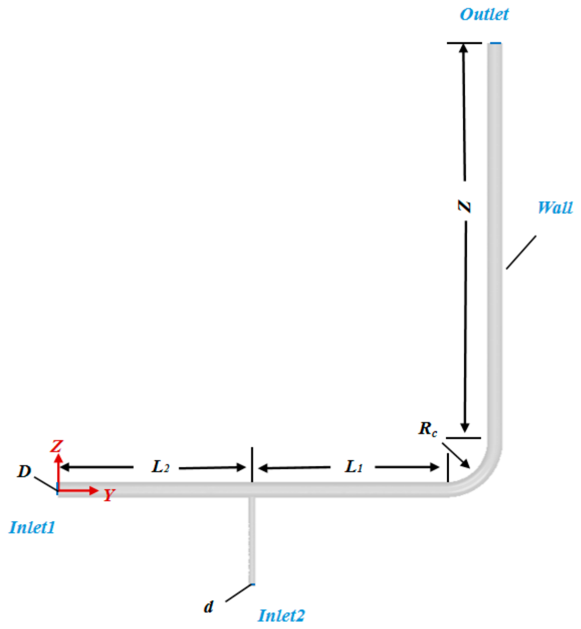
Figure 1 shows a schematic diagram of the hydrogen-blended natural gas pipe. Methane gas is introduced through Inlet 1, while hydrogen gas is introduced through the lower Inlet 2. The main pipeline dimensions from the China Power Investment Corporation Chaoyang Natural Gas Hydrogen Blending Demonstration Project pipeline network were used: D = 0.8 m, hydrogen inlet diameter 0.32 m, and total upstream pipeline length 20 m. L₁ denotes the distance from the center of the hydrogen injection branch to the elbow inlet. L₂ denotes the distance from Inlet 1 to the branch center and is adjusted so that the total upstream straight-pipe length remains 20 m. Although they vary simultaneously to maintain a constant total upstream length, the incoming-flow conditions immediately upstream of the hydrogen injection branch remain essentially unchanged among the investigated cases. This arrangement maintains the same overall flow-development distance from the main inlet to the elbow for all the configurations, providing a consistent pipe length for comparing the mixing behaviors of the elbows with different hydrogen-injection layouts.

2.2. Numerical Method

Three-dimensional numerical simulations of hydrogen-natural gas mixing in the pipeline were performed using ANSYS FLUENT 17. The continuity equation is as follows:

$$\begin{array}{c}{\displaystyle \frac{\partial \rho }{\partial t}}+\nabla \cdot \left(\rho \mathbf{u}\right)=0\end{array}$$

(1)

where ρ is the density of the gas mixture, t is the time, and u is the flow vector field.

The momentum equation is represented by:

$$\begin{array}{c}{\displaystyle \frac{\partial \left(\overline{\rho }{u}_i\right)}{\partial t}}+{\displaystyle \frac{\partial \left(\overline{\rho }{u}_i{u}_j\right)}{\partial x_j}}=-{\displaystyle \frac{\partial p}{\partial x_i}}+{\displaystyle \frac{\partial }{\partial x_j}}\left({\mu }_e\left({\displaystyle \frac{\partial u_i}{\partial x_j}}+{\displaystyle \frac{\partial u_j}{\partial x_i}}\right)\right)+\overline{\rho }{f}_i\end{array}$$

(2)

where pressure is denoted by p, effective dynamic viscosity by μ_e, and f_i represents the gravitational force acting on the fluid.

The energy conservation equation is as follows:

$$\begin{array}{c}{\displaystyle \frac{\partial \left(\rho c_{p}T\right)}{\partial t}}+{\displaystyle \frac{\partial \left(\rho c_p{u}_{j}T\right)}{\partial x_j}}={\displaystyle \frac{\partial }{\partial x_j}}\left(\lambda {\displaystyle \frac{\partial T}{\partial x_j}}\right)+S\end{array}$$

(3)

where T is the mixture temperature, c_p is the specific heat capacity at constant pressure, λ is the effective thermal conductivity, and S represents the volumetric energy source term.

The equation governing species transport can be expressed as follows:

$$\begin{array}{c}{\displaystyle \frac{\partial \left(\rho c_s\right)}{\partial t}}+{\displaystyle \frac{\partial }{\partial x_j}}\left(\rho u_j{c}_s\right)={\displaystyle \frac{\partial }{\partial x_j}}\left(D_s\rho {\displaystyle \frac{\partial c_s}{\partial x_j}}\right)\end{array}$$

(4)

where c_s denotes the concentration of species s. Following the species-transport formulation adopted in our previous study [22], the diffusive transport in turbulent flow includes both molecular diffusion and turbulence-induced species diffusion. The turbulent contribution is characterized by the turbulent Schmidt number, with S_ct = 0.7 adopted in the present simulations. For molecular diffusion, the constant-dilute approximation was adopted, and the molecular diffusivity of hydrogen in methane was set to 2.88 × 10⁻⁵ m²/s.

This paper introduces the coefficient of variation (COV) as a means of assessing the uniformity of hydrogen and natural gas mixing in pipelines. A lower COV indicates a more homogeneous mixture. In this study, a COV threshold of 0.05 is adopted as the criterion for homogeneous mixing.

$$\begin{array}{c}COV={\displaystyle \frac{1}{\overline{c}}}\sqrt{{\displaystyle \frac{{\displaystyle {\sum }_{i=1}^n} {\left(c_i-\overline{c}\right)}^2}{n-1}}}\end{array}$$

(5)

where c_i is the hydrogen mole fraction at the ith monitoring point, $\overline{c}$ is the average hydrogen mole fraction over the monitored cross-section, and n is the total number of computational sampling points on the corresponding cross-section. The hydrogen mole fractions at all the sampling points distributed over the entire cross-section were extracted for the COV calculation.

Given the specified hydrogen blending ratio (HBR), the required hydrogen inlet velocity can be calculated as follows:

$$\begin{array}{c}{\displaystyle \frac{v_{{\mathrm{H}}_2}}{v_{{\mathrm{C}\mathrm{H}}_4}}}={\left({\displaystyle \frac{D}{d}}\right)}^2\cdot {\displaystyle \frac{\mathrm{H}\mathrm{B}\mathrm{R}}{1-\mathrm{H}\mathrm{B}\mathrm{R}}}\end{array}$$

(6)

where v_H2 denotes the flow velocity of hydrogen, v_CH4 represents the flow velocity of methane, D indicates the cross-sectional diameter of the natural gas pipeline, d denotes the diameter of the branch pipeline, and HBR measures the blending ratio of hydrogen in the mixed gas.

The standard k-ε model was adopted to predict the global concentration-mixing characteristics because it provides a practical balance between computational cost and accuracy for turbulent pipeline flows [35].

The present analysis therefore focuses primarily on integral quantities, including COV and the homogeneous mixing path. Although the standard k-ε model has limitations in resolving detailed turbulence anisotropy, it has been widely applied to steady turbulent flows in 90° pipe bends for predicting the principal mean-flow redistribution and curvature-induced secondary-flow characteristics.

$$\begin{array}{c}{\displaystyle \frac{\partial }{\partial t}}\left(\rho k\right)+{\displaystyle \frac{\partial }{\partial x_i}}\left(\rho u_{i}k\right)={\displaystyle \frac{\partial }{\partial x_j}}\left[\left(\mu +{\displaystyle \frac{{\mu }_t}{{\sigma }_k}}\right){\displaystyle \frac{\partial k}{\partial x_j}}\right]+G_K+G_b-\rho \epsilon -Y_M+S_k\end{array}$$

(7)

$$\begin{array}{c}{\displaystyle \frac{\partial }{\partial t}}\left(\rho \epsilon \right)+{\displaystyle \frac{\partial }{\partial x_i}}\left(\rho u_i\epsilon \right)={\displaystyle \frac{\partial }{\partial x_j}}\left[\left(\mu +{\displaystyle \frac{{\mu }_t}{{\sigma }_{\epsilon }}}\right){\displaystyle \frac{\partial \epsilon }{\partial x_j}}\right]+C_{1\epsilon }{\displaystyle \frac{\epsilon }{k}}\left(G_K+C_{3\epsilon }{G}_b\right)-C_{2\epsilon }\rho {\displaystyle \frac{{\epsilon }^2}{k}}+S_{\epsilon }\end{array}$$

(8)

where Y_M represents the contribution of fluctuating dilatation in compressible turbulence to the overall dissipation rate, and G_k and G_b denote the turbulent kinetic energy generated by the mean velocity gradient and buoyancy, respectively.

The simulations were performed using a steady-state pressure-based solver. The gas mixture density was calculated using the incompressible ideal-gas law, and the thermophysical properties of methane and hydrogen were obtained from the ANSYS Fluent material database. The mixture specific heat was evaluated using the mixing law. Gravity was set to 9.81 m/s² in the negative z-direction, and the pipe walls were treated as adiabatic. The SIMPLEC algorithm was employed for pressure–velocity coupling. Second-order pressure interpolation was used, while the momentum, energy, and species transport equations were discretized using the second-order upwind scheme. The turbulent kinetic energy and turbulent dissipation rate equations were discretized using the first-order upwind scheme. The under-relaxation factors were 1.0 for pressure correction, 0.7 for momentum, 0.8 for k and ε, and 1.0 for energy and species transport. Convergence was considered to be achieved when the residuals of all the governing equations decreased below 1 × 10⁻⁵ and the monitored flow and species quantities remained stable. After convergence, the overall mass imbalance was approximately 0.061%, while the species imbalances of H₂ and CH₄ were approximately 0.0006% and 0.00019%, respectively, indicating satisfactory mass and species conservation.

2.3. Boundary Conditions

Because methane is the principal component of natural gas, it was used as a surrogate for natural gas in the present simulations [36]. The methane and hydrogen boundaries were specified as velocity inlets. A turbulence intensity of 5% was specified at both velocity inlets, and the hydraulic diameter was used as the characteristic length scale. The hydraulic diameters were 0.8 m for the methane inlet and 0.32 m for the hydrogen inlet, while the outlet was specified as a pressure outlet at 1.8 MPa. In this study, we focus on the intermediate pressure section (approx. 1.8 MPa) typically found in the riser base or downstream processing units of offshore platforms, where mixing uniformity is critical before further processing. The methane inlet velocity was set to 5 m/s. A hydrogen blending ratio of 25% by volume was considered in the present study. The target HBR was imposed through the inlet velocities and cross-sectional areas rather than by specifying mass-flow fractions. The selected hydrogen blending ratio is within the range investigated in previous hydrogen-natural gas studies [37,38]. The temperatures of both gas streams were set to 300 K, and the detailed boundary conditions are summarized in

Table 1. Details of the boundary conditions.

Boundary	Type of Boundary Condition	Parameter Values
Inlet 1	Velocity inlet	5 m/s
Inlet 2	Velocity inlet	10.42 m/s
Outlet	Pressure outlet	1.8 MPa
Wall	Wall	No-slip wall, roughness height = 0 m

.

2.4. Verification and Validation

2.4.1. Grid Independence Study

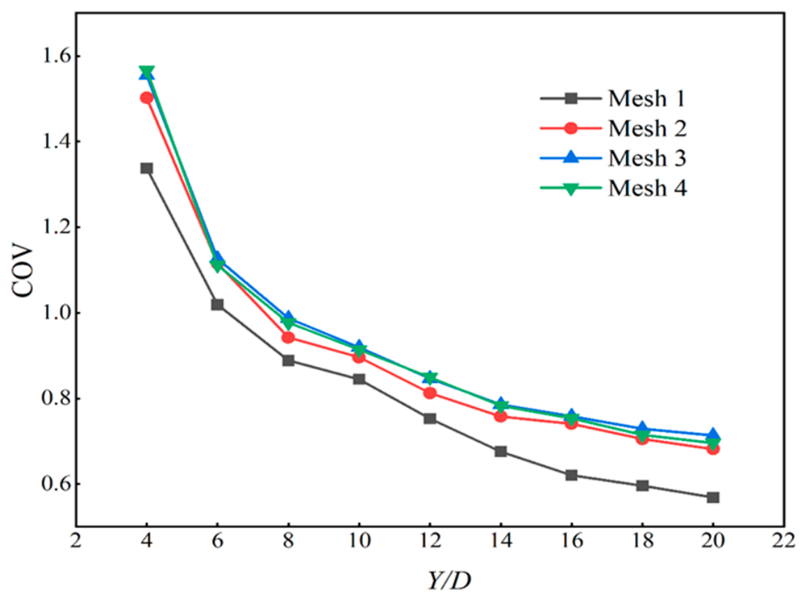
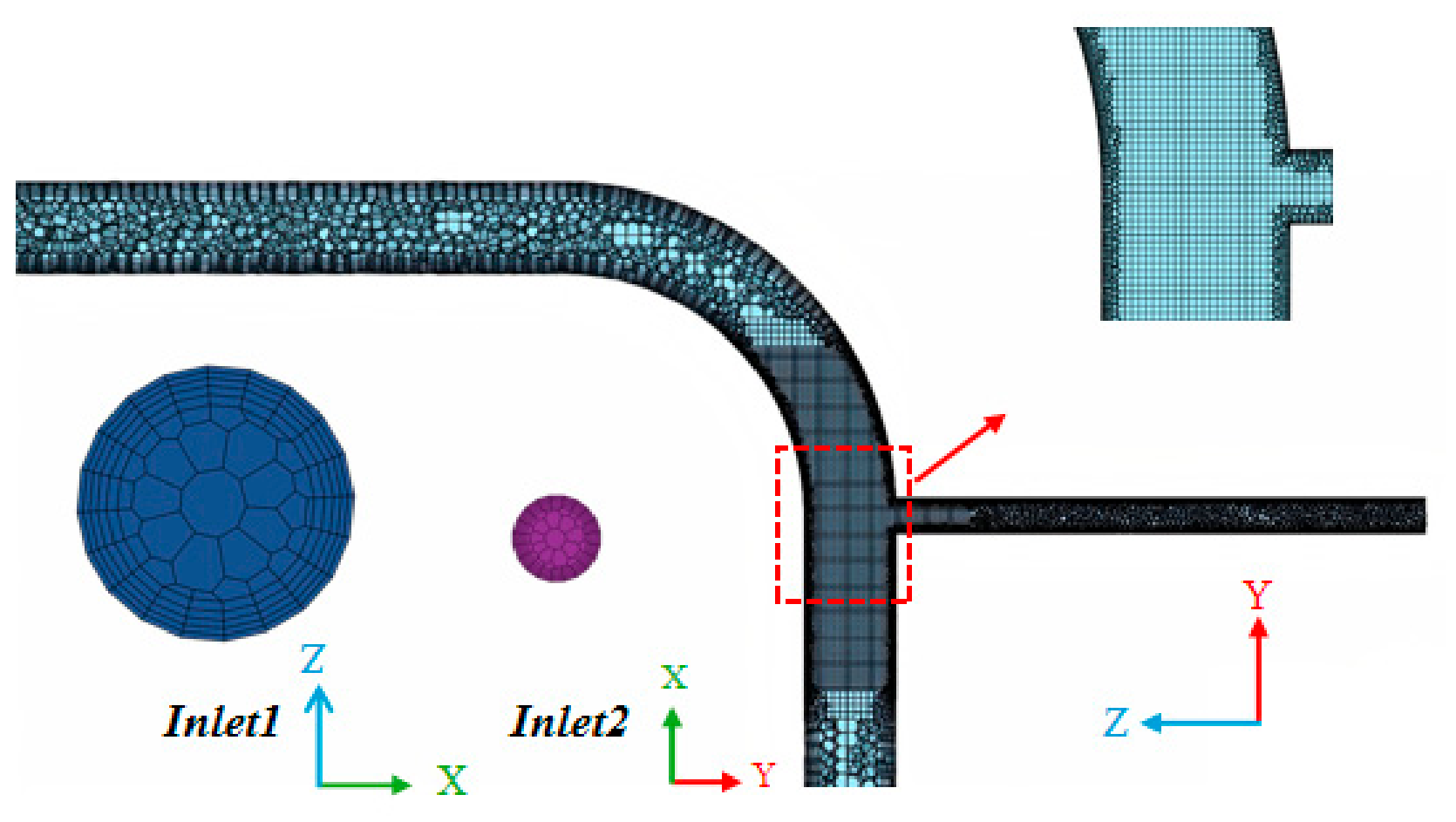
These grids were constructed through ANSYS FLUENT software, employing tetrahedral and hexahedral partitioning methods to divide the computational domain. Local mesh refinement was applied near the branch junction, elbow, and pipe walls to improve the resolution of the local velocity and concentration gradients. Standard Wall Functions were employed for the near-wall treatment in conjunction with the standard k-ε model. The wall y⁺ values over the main-pipe and elbow surfaces were maintained within the recommended range for Standard Wall Functions, ensuring appropriate near-wall resolution for the present turbulent flow simulations. Figure 2 shows a cross-section of the pipeline, illustrating the internal mesh and wall details.

Table 2. Mesh quality of grid independence study.

Mesh No.	Grid Number	Maximum Skewness	Minimum Orthogonality Quality	Maximum Aspect Ratio
Mesh 1	57,828	0.58	0.42	26.90
Mesh 2	136,312	0.48	0.52	15.67
Mesh 3	227,311	0.49	0.51	15.30
Mesh 4	402,648	0.50	0.50	15.31

displays the quality details of all mesh quantities. Figure 3 shows the variation in COV along different distance directions in the natural gas pipeline cross-section after mixing at different mesh counts. The COV profiles obtained with Meshes 3 and 4 are nearly coincident. Quantitatively, the average relative difference in COV between the two meshes over all the monitored cross-sections is only 1.37%. For the configuration subsequently identified as the optimal case (L₁ = 0, R_c/D = 4), the homogeneous mixing paths predicted using Mesh 3 and Mesh 4 were 11.73 m and 11.42 m, respectively, based on the same homogeneous-mixing criterion of COV ≤ 0.05. Taking Mesh 4 as the reference, the relative difference in S_h was approximately 2.71%. These results indicate that further grid refinement has only a limited influence on both the predicted concentration field and the homogeneous mixing path. Therefore, Mesh 3 was selected for the subsequent simulations considering both numerical accuracy and computational cost.

To evaluate the influence of turbulence-model selection on the predicted mixing performance, an additional RSM simulation was conducted for the representative configuration (L₁ = 0 m, R_c/D = 4). The COV at the elbow outlet predicted by the standard k-ε model and RSM was 0.556 and 0.573, respectively. The corresponding homogeneous mixing paths were 11.73 m and 12.57 m. The difference between the two predictions was 0.84 m, corresponding to a relative deviation of 2.34% with respect to the conventional T-pipe mixing path. This indicates that the turbulence-model selection has a limited influence on the relative mixing enhancement caused by the branch–elbow configuration. Considering the higher computational cost of RSM, the standard k-ε model was adopted for the subsequent parametric study.

2.4.2. Validation of Numerical Method

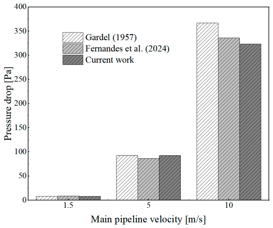
To assess the numerical model, the predicted pressure drops were compared with the Gardel correlation [34] and the results reported by Fernandes et al. [33].

$$\begin{array}{c}{K}_{31}=-0.92{\left(1-q\right)}^2-q^2\left(1.2-r^{0.5}\right)\left(\cos \left({\displaystyle \frac{\theta }{a}}\right)-1\right)+0.8q^2\left(1-{\displaystyle \frac{1}{a^2}}\right)-\\ 0.8q^2\left({\displaystyle \frac{1}{a}}-1\right)\cos \left(\theta \right)+\left(2-a\right)\left(1-q\right)q\end{array}$$

(9)

$$\begin{array}{c}{K}_{32}=0.03\left(1-q^2\right)-q^2\left[1+\left(1.62-r^{0.5}\right)\left(\cos \left({\displaystyle \frac{\theta }{a}}\right)-1\right)-0.38\left(1-a\right)\right]\\ +\left(2-a\right)\left(1-q\right)q\end{array}$$

(10)

where a, q, r, and θ represent the area ratio between the branch pipe and the main pipe, the flow ratio, the dimensionless radius ratio at the branch-to-main junction, and the angle between the two pipes, respectively.

As shown in Figure 4, the predicted pressure drops show reasonable agreement with the Gardel correlation and the results reported by Fernandes et al. [33] supporting the model’s ability to reproduce the global hydraulic losses of the injection configuration. Together with the grid-independence assessment, this comparison provides a numerical basis for the subsequent analysis of hydrogen transport and mixing characteristics. The pressure-drop comparison assesses the global hydraulic response and does not directly validate the local concentration field or detailed secondary-flow structures. Therefore, COV and the homogeneous mixing path are used as the primary indicators for comparing mixing performance among different configurations.

3. Results and Discussions

This section analyzes the gas mixing characteristics for four branch-to-elbow distances and identifies the configuration with the shortest homogeneous mixing path by comparing different curvature-radius ratios. The COV and the homogeneous mixing path S_h are used to quantify cross-sectional concentration uniformity and the downstream path required to achieve homogeneous mixing. Here, S_h is defined as the centerline distance from the hydrogen injection section to the first downstream cross-section at which the COV decreases to 0.05. The flow field evolution mechanisms of two structures with outstanding mixing performance were elucidated through qualitative analysis of streamlines and hydrogen distribution across the pipe cross-section, coupled with quantitative analysis of the cross-sectional average vorticity parameter.

3.1. Effect of Distance Between the Branch and Elbow Inlet

In this section, numerical studies were conducted on elbow structures with varying distances between the branch and elbow inlet (L₁ = 0 m,5 m,10 m,15 m) at a fixed curvature-radius ratio of R_c/D = 3. These simulations reveal the flow and mixing characteristics and clarify the influence of the upstream flow-field development state on the downstream secondary flow.

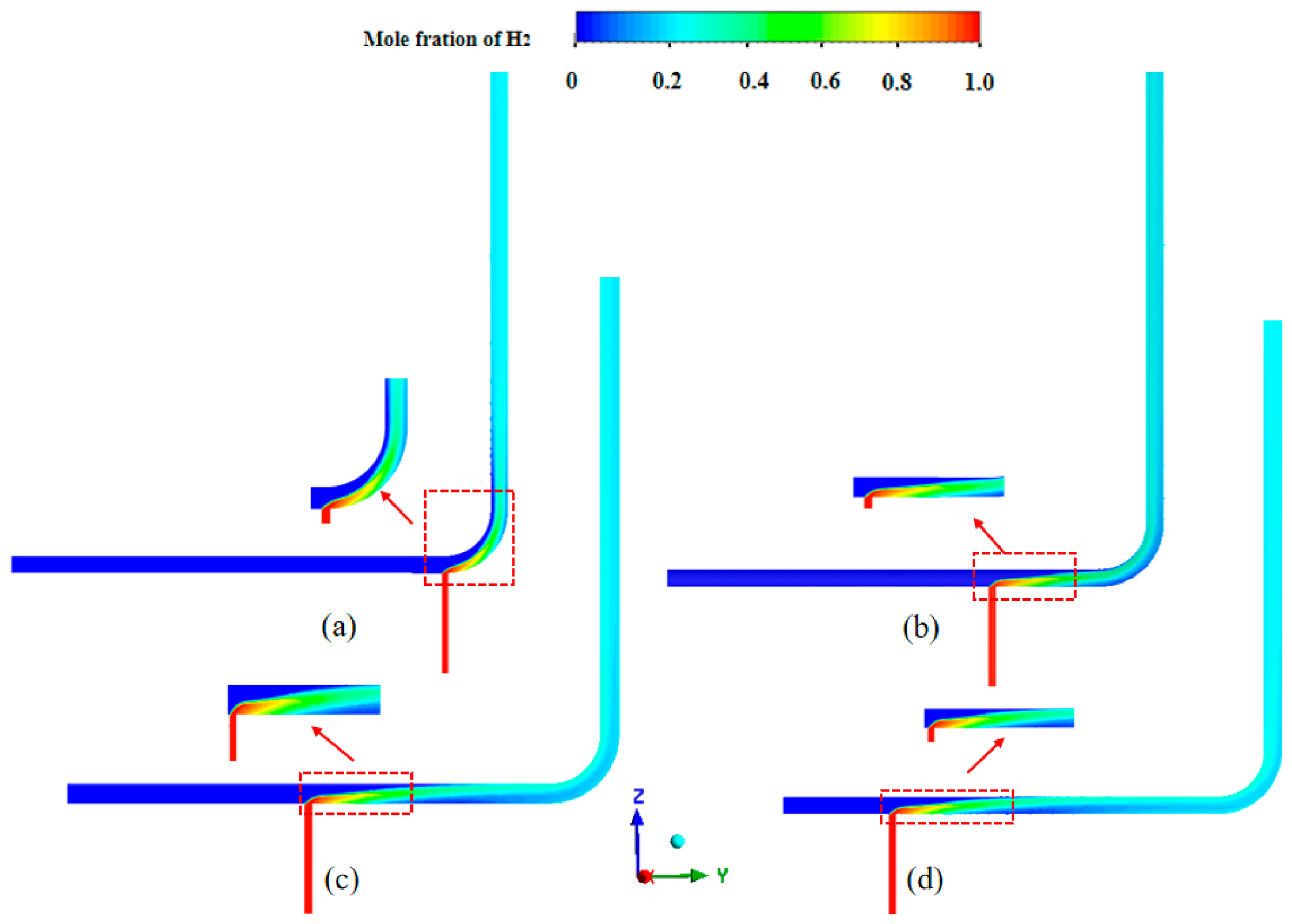
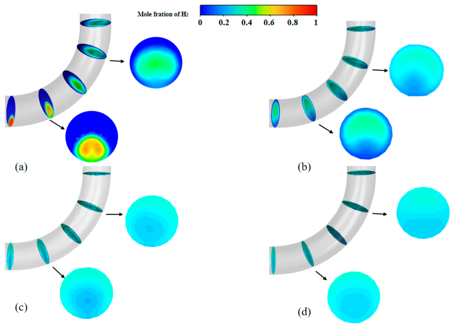
Figure 5 intuitively shows the spatial distribution characteristics of hydrogen molar fraction under different L₁. The hydrogen mole fraction distributions show that hydrogen injected through Inlet 2 initially accumulates near the lower part of the main pipe and subsequently spreads toward the pipe core and upper region. Specifically, Figure 5c,d show that hydrogen needs to travel a certain distance to complete the upward layered diffusion process, while Figure 5a,b show that hydrogen can diffuse to the center of the pipe in a short time.

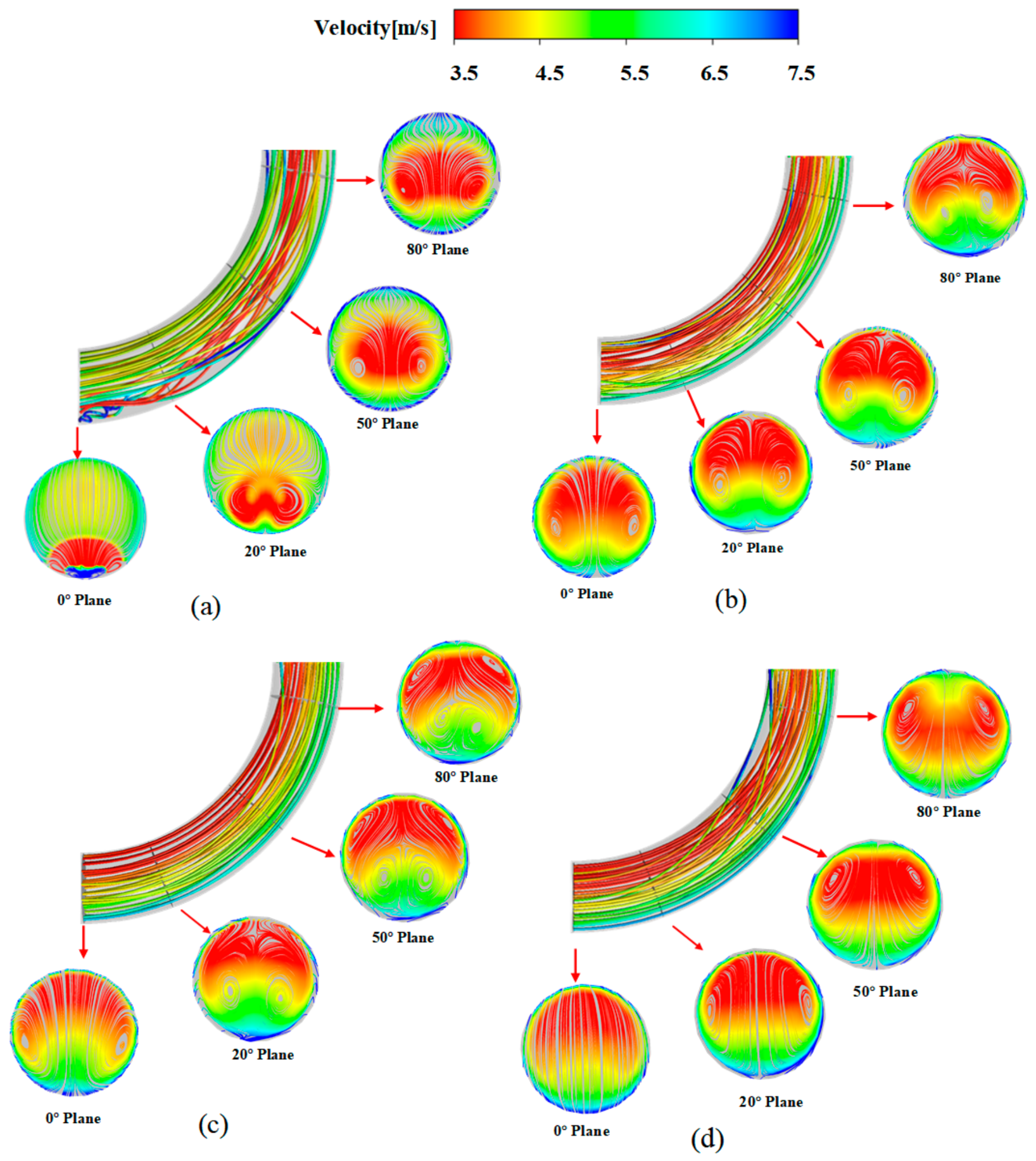
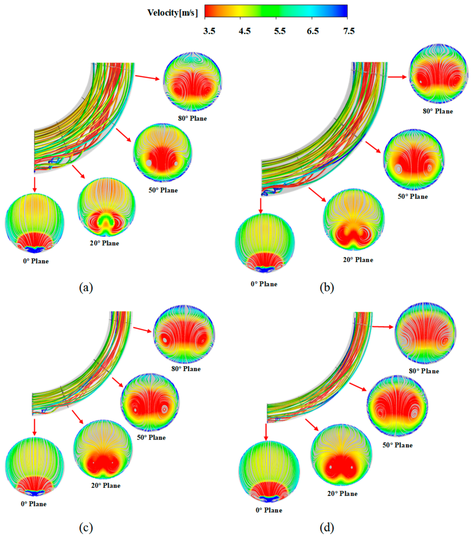
Figure 6 shows the flow field details of the elbow section at different distances between the branch and elbow inlet when R_c/D = 3. At L₁ = 0 m, the streamlines of the straight pipe section are severely entangled. In the elbow area, high-speed streamlines are concentrated in the center of the flow channel, while low-speed streamlines are squeezed to the outside and continuously twisted. The secondary flow is initially characterized by a primary vortex pair, with an additional vortex pair developing near the elbow exit. At L₁ = 5 m, the disturbance in the upstream straight section is weaker than that at L₁ = 0 m, but the high-speed flow lines in the bend area tend to turn inward, and there are still low-speed flow lines entangled on the outside. The flow field in the cross-section is a double vortex when the bend angle is small, and an additional pair of high-speed vortices appears on the inside at 80°. At L₁ = 10 m, the flow lines in the straight pipe section are smooth and layered, and the flow lines in the bending zone transition naturally without obvious entanglement or high-speed flow line deviation. A pair of high-speed vortices forms on the inner side at a bend angle of 50°, and the high-speed vortices continue to grow at 80°. At L₁ = 15 m, the flow lines in the straight pipe section are straight, but there are slight fluctuations in the low-speed flow lines in the local area of the curved section. Figure 7 illustrates the molar fraction distribution of hydrogen under different L₁, presenting a cloud view of the cross-sectional hydrogen distribution within the different pipeline configurations.

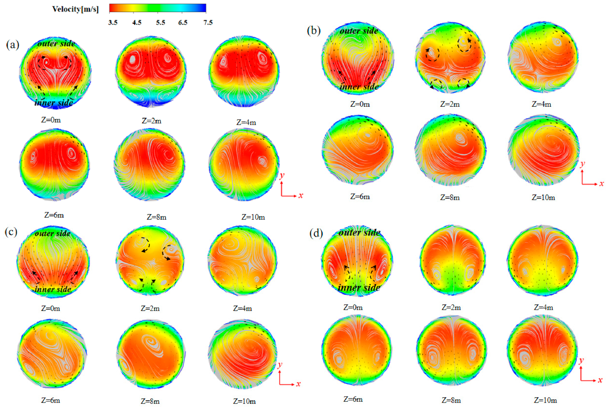
Figure 8 compares the downstream evolution of the cross-sectional flow fields for different L₁ values. At L₁ = 0 m, a transient four-vortex structure is observed at the elbow outlet (Z = 0 m), consisting of a primary Dean-vortex pair and an additional outer vortex pair. The outer vortices decay within approximately 3 m downstream. At L₁ = 5 m, the outer vortices also appear but become unstable and gradually merge downstream. At L₁ = 10 m, the vortex structure evolves from four vortices at Z = 2 m to three vortices at Z = 4 m, two vortices at Z = 6 m, and a single dominant vortex at Z = 10 m. In contrast, a relatively stable double-vortex structure persists downstream at L₁ = 15 m. These differences indicate that the inlet-flow condition influences the development and downstream reorganization of the elbow-induced mean secondary-flow structures.

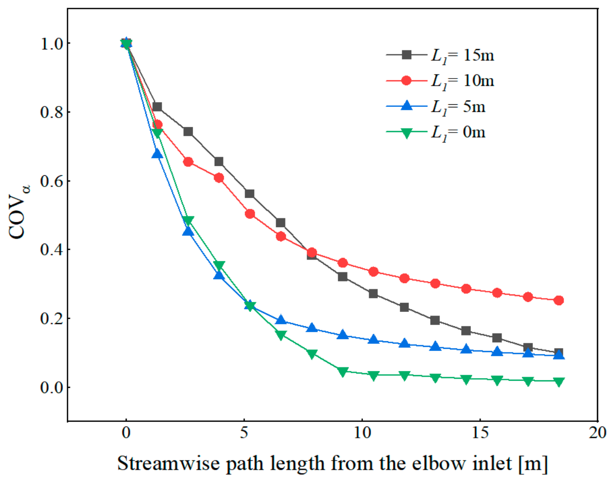
To compare the evolution of hydrogen concentration uniformity among different L₁ configurations, the normalized coefficient of variation is defined as:

$$\begin{array}{c}{\mathrm{COV}}_{\mathrm{\alpha }}={\displaystyle \frac{\mathrm{C}\mathrm{O}\mathrm{V}}{\mathrm{C}\mathrm{O}{\mathrm{V}}_0}}\end{array}$$

(11)

where COV is the coefficient of variation at a given cross-section, and COV₀ is the coefficient of variation at the elbow inlet of the corresponding configuration. The elbow inlet is taken as the reference position, i.e., s = 0. Therefore, COV_α = 1 at the elbow inlet, and a lower COV_α indicates a greater improvement in hydrogen concentration uniformity along the elbow and downstream pipe.

Figure 9 shows the variation of COV_α with the streamwise path length measured from the elbow inlet for different L₁ configurations. For all L₁ configurations, COV_α decreases with increasing streamwise path length from the elbow inlet, indicating a progressive improvement in cross-sectional hydrogen concentration uniformity. Within the first 5 m from the elbow inlet, COV_α decreases rapidly because of curvature-induced secondary motion and subsequent vortex reorganization; beyond a downstream path length of approximately 5 m, the decrease in COV_α gradually becomes less pronounced, indicating that the flow field parameters gradually reach a stable state. The different L₁ values have a significant influence on the downstream mixing characteristics. The L₁ = 0 m configuration exhibits the steepest initial decrease in COV_α, indicating that the undeveloped inlet flow strengthens the mixing disturbance within the elbow. Conversely, a longer upstream development length produces a more developed inlet flow and weakens the additional disturbance generated by the elbow.

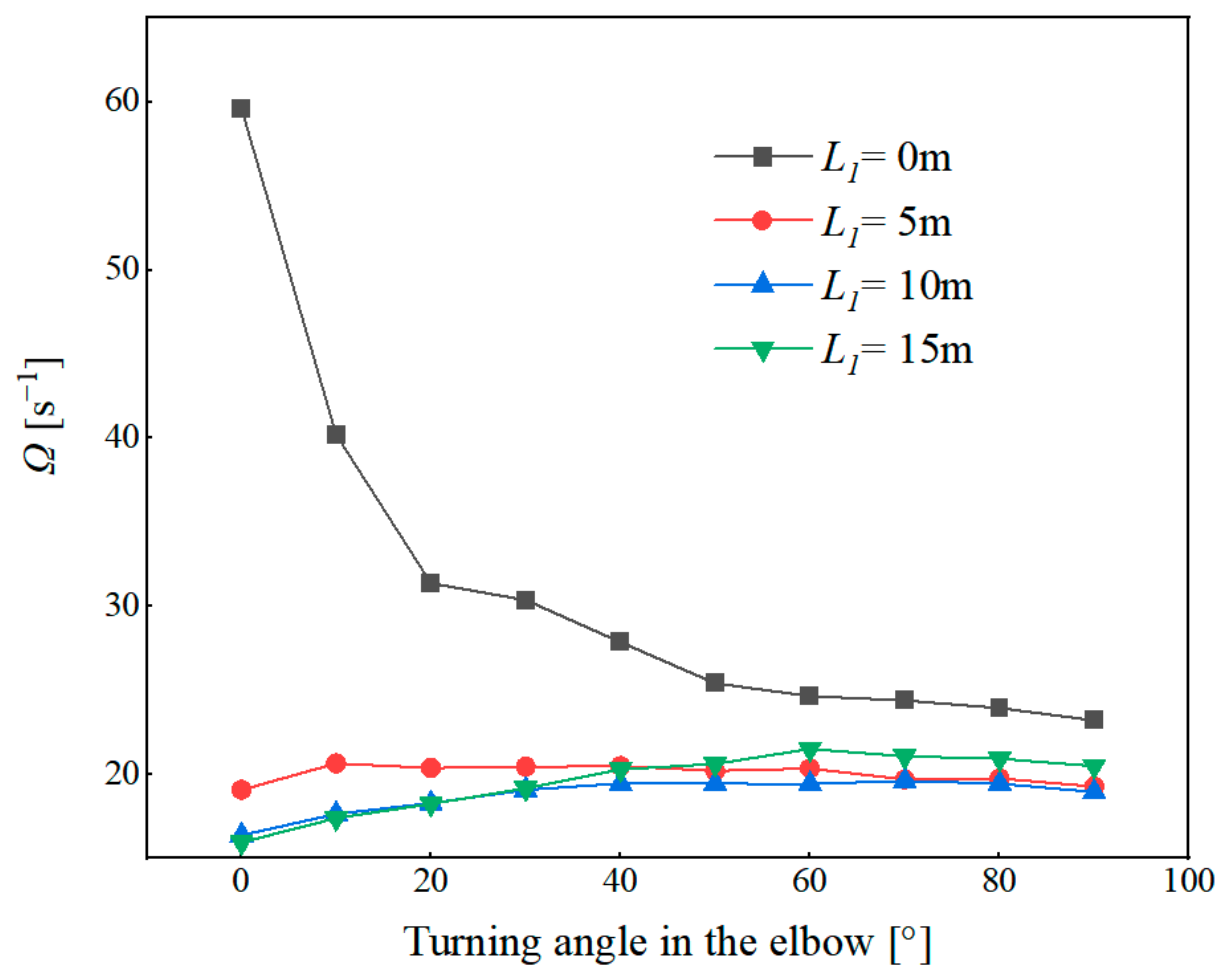
To quantify the disturbance inside the four types of elbow structures, the area-averaged vorticity is introduced for evaluation, which can be defined as:

$$\begin{array}{c}⟨\Omega ⟩={\displaystyle \frac{1}{A}}{\int }_A \Omega dA\end{array}$$

(12)

where ⟨Ω⟩ represents the cross-sectional area-averaged vorticity magnitude, A is the cross-sectional area, and Ω denotes the local vorticity magnitude.

Figure 10 shows that the development length in the upstream is a key factor affecting the vorticity values in the elbow. Taking L₁ = 0 m as an example, due to insufficient upstream flow field development, the velocity gradient distribution is disordered, and violent disturbances are generated under the action of centrifugal force, resulting in an initial vorticity value as high as 60 s⁻¹. This also explains the reason for the intense flow field entanglement observed in Figure 6a. In contrast, under L₁ = 15 m, the upstream flow field is fully developed, the velocity distribution is uniform, and the disturbance effect of the elbow is weak. As the turning angle in the elbow increases, the difference in vorticity between the various L₁ values gradually decreases, with the vorticity under L₁ = 0 m rapidly decaying, while the 5 m, 10 m, and 15 m show a converging trend. This convergence indicates that the influence of the inlet-flow condition gradually weakens along the elbow, while curvature and wall confinement increasingly govern the downstream evolution of the secondary-flow field. Regardless of the initial flow field conditions, during the continuous bending flow process, the fluid is affected by the combined effects of elbow curvature and wall friction, and the vortex structure undergoes a process of dissipation and reorganization, ultimately achieving stable convergence of the vorticity distribution.

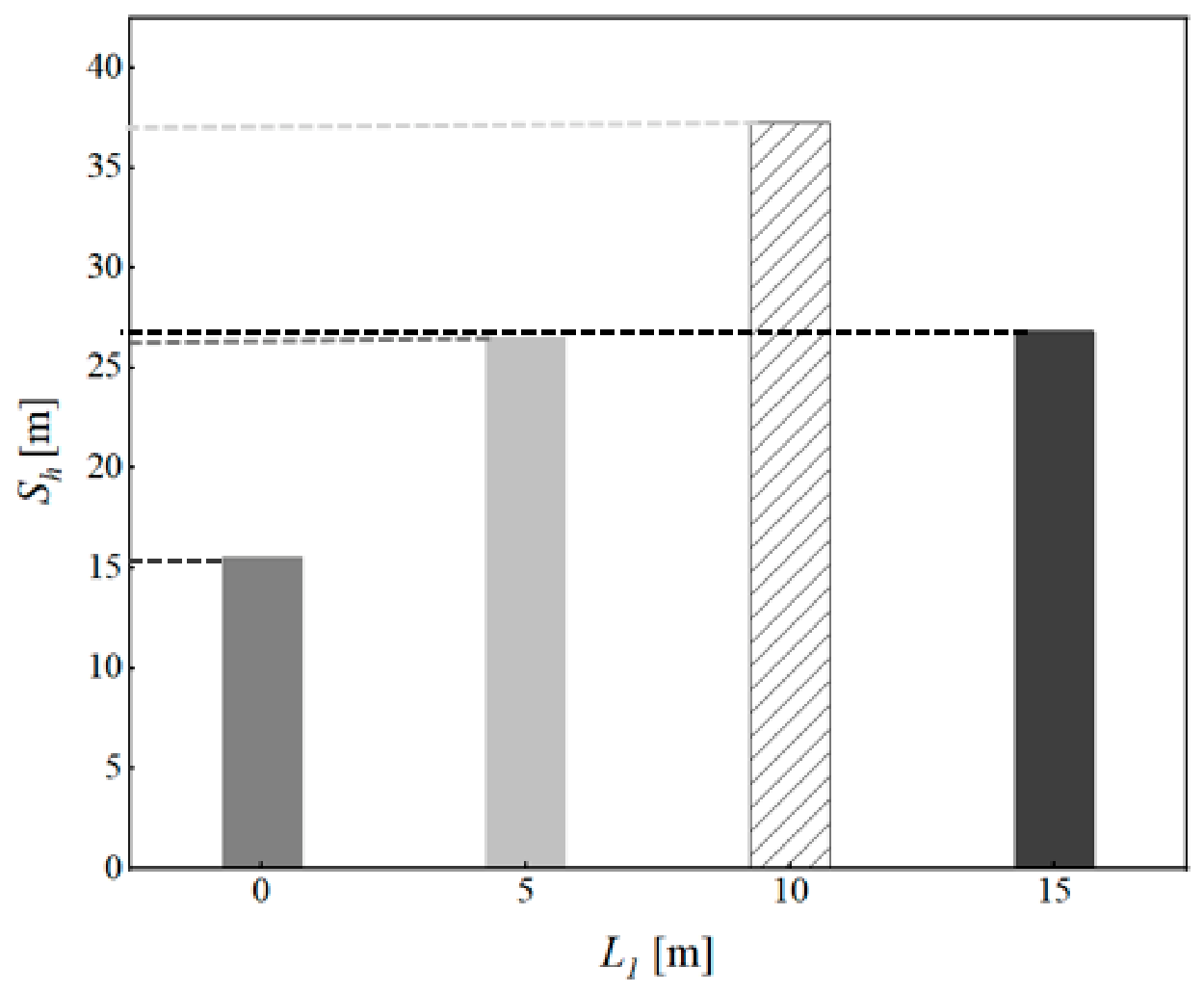
Figure 11 compares the homogeneous mixing paths S_h for different L₁ values. The corresponding S_h values are 15.53 m, 26.53 m, 37.23 m, and 26.83 m for L₁ = 0 m, 5 m, 10 m, and 15 m, respectively, showing a non-monotonic dependence on L₁. When L₁ is short, the flow field disturbance is significant, and the mixing speed is accelerated; when L₁ is moderate, the flow field stability is high, but a longer distance is needed to achieve full mixing. The decrease in S_h from L₁ = 10 m to L₁ = 15 m is mainly due to greater pre-elbow hydrogen redistribution, which partially offsets the weaker elbow-induced mixing. It is found that L₁ affects the mixing process of the hydrogen-blended natural gas pipeline downstream of the elbow by changing the initial conditions of the flow field, and the structure of the flow field changes significantly under the combined effect of centrifugal force and secondary vortices when the fluid flows through the elbow region. The curvature-induced redistribution of the velocity field strengthens transverse convection and shear-enhanced species transport, thereby disrupting the initially non-uniform hydrogen distribution and accelerating hydrogen transport toward the pipe core. For short L₁, mixing is strongly influenced by the interaction between the undeveloped injection flow and the elbow-induced secondary flow. As L₁ increases, this interaction weakens, while upstream turbulent transport contributes more substantially to the concentration redistribution before the mixture enters the elbow.

3.2. Effect of Curvature Radius

This section conducts a numerical study of structures with R_c/D = 2, 3, 4, and 5, where R_c is the curvature radius of the turn, revealing the effects of different curvature-radius ratios on mixing and downstream flow characteristics.

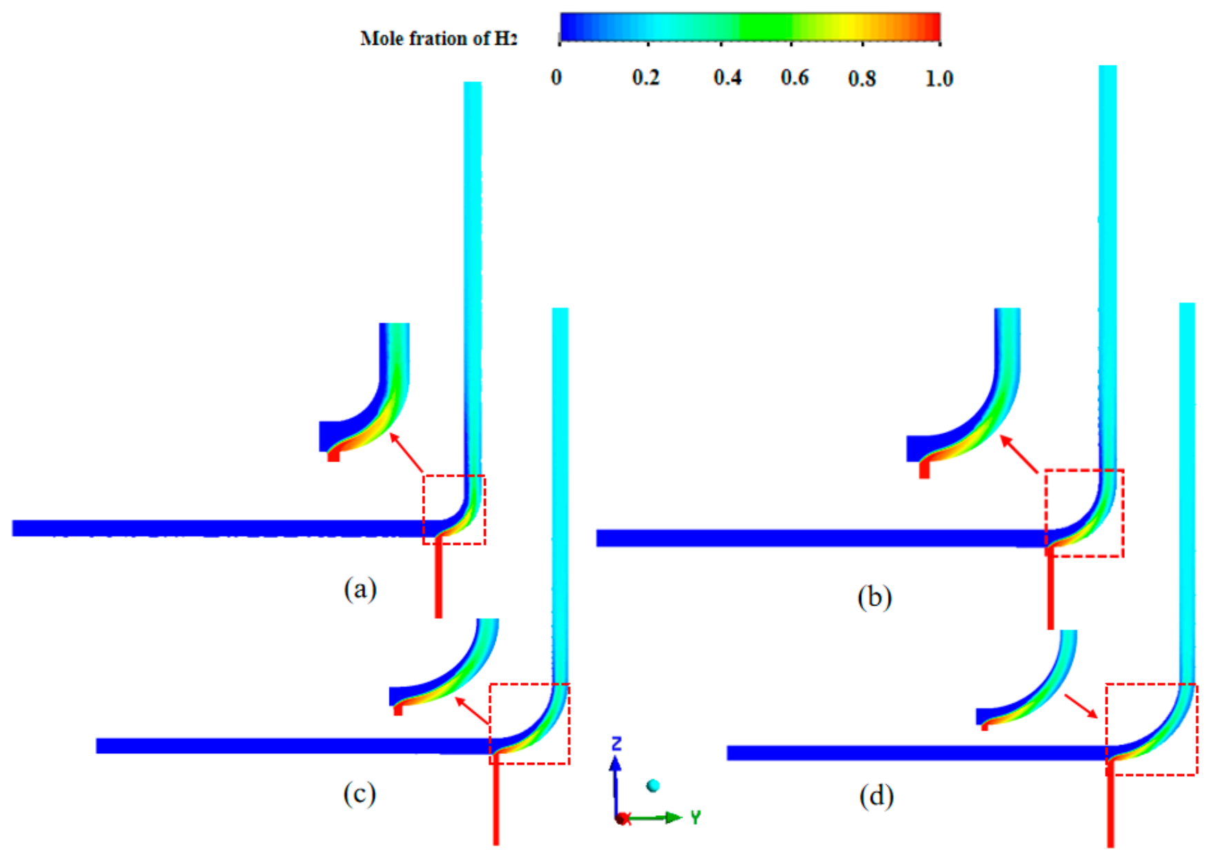
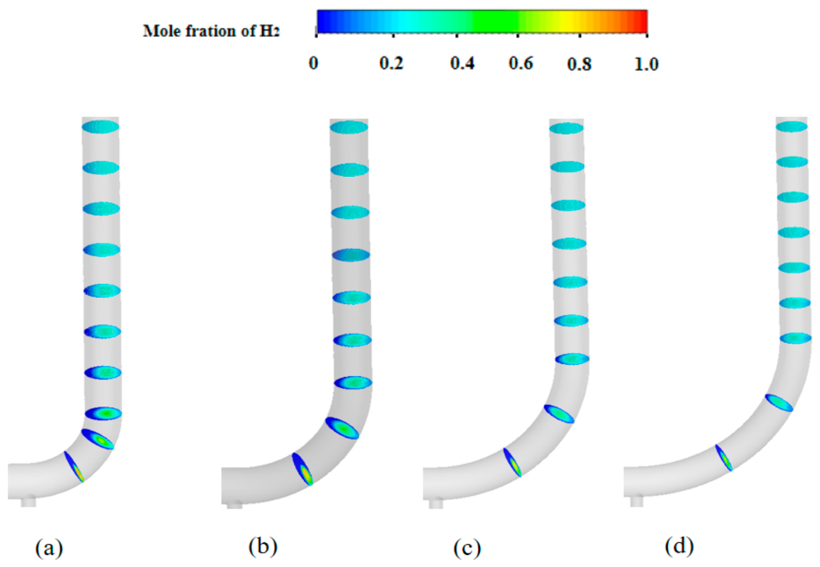
Figure 12 intuitively shows the spatial distribution characteristics of the hydrogen mole fraction under different curvature radii. In Figure 12a, the hydrogen plume is strongly deflected toward the right side after entering the elbow. Its interaction with the stronger curvature-induced secondary flow produces a highly asymmetric concentration distribution and a distinct local enrichment region. For R_c/D = 3–5, the hydrogen concentration distribution becomes progressively less asymmetric, with a reduced local enrichment region and enhanced transport toward the opposite side of the cross-section.

Figure 13 shows the streamlines in elbow sections with different curvature radii. It can be seen that the streamlines are severely entangled at small turning angles in the elbow. Under R_c/D = 2, 3, and 4, the high-speed region is located at the center of the pipe. At R_c/D = 5, the high-speed region shifts toward the inner arc surface. This change is associated with the weakening of curvature-induced centrifugal effects, which increases the relative influence of buoyancy on hydrogen redistribution [12]. At R_c/D = 2, a pair of outer vortices appears at 80°, which is caused by the elbow. At R_c/D = 3, 4 and 5, the cross-section is a double-vortex Dean structure.

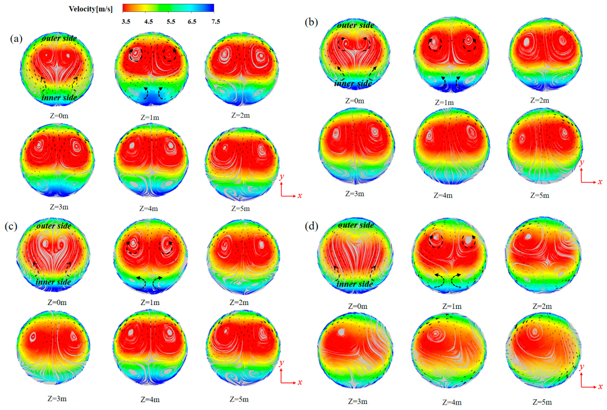
To further study the effect of different curvatures on downstream flow, Figure 14 shows the flow field downstream of four elbow radii. All four structures exhibit outer Dean vortices, but the size and location of their disappearance vary. The outer vortices have opposite velocity directions to the inner vortices, and at R_c/D = 2 and 3, they disappear at 4 m downstream, with the outer Dean vortices occupying one-third of the space. At R_c/D = 4, the outer vortex decreases in size and shows a tendency to disappear at 3 m downstream, subsequently forming a stable double vortex structure. At R_c/D = 5, the outer vortex and base vortex are evenly divided at 1 m downstream, forming a triple vortex structure at 3 m downstream. At 4 m downstream, it becomes a two-vortex structure, and at 5 m downstream, it becomes a single-vortex structure. From the perspective of the velocity field, the outer vortex is a low-speed vortex. The research results show that changes in curvature will cause the downstream flow field to redistribute.

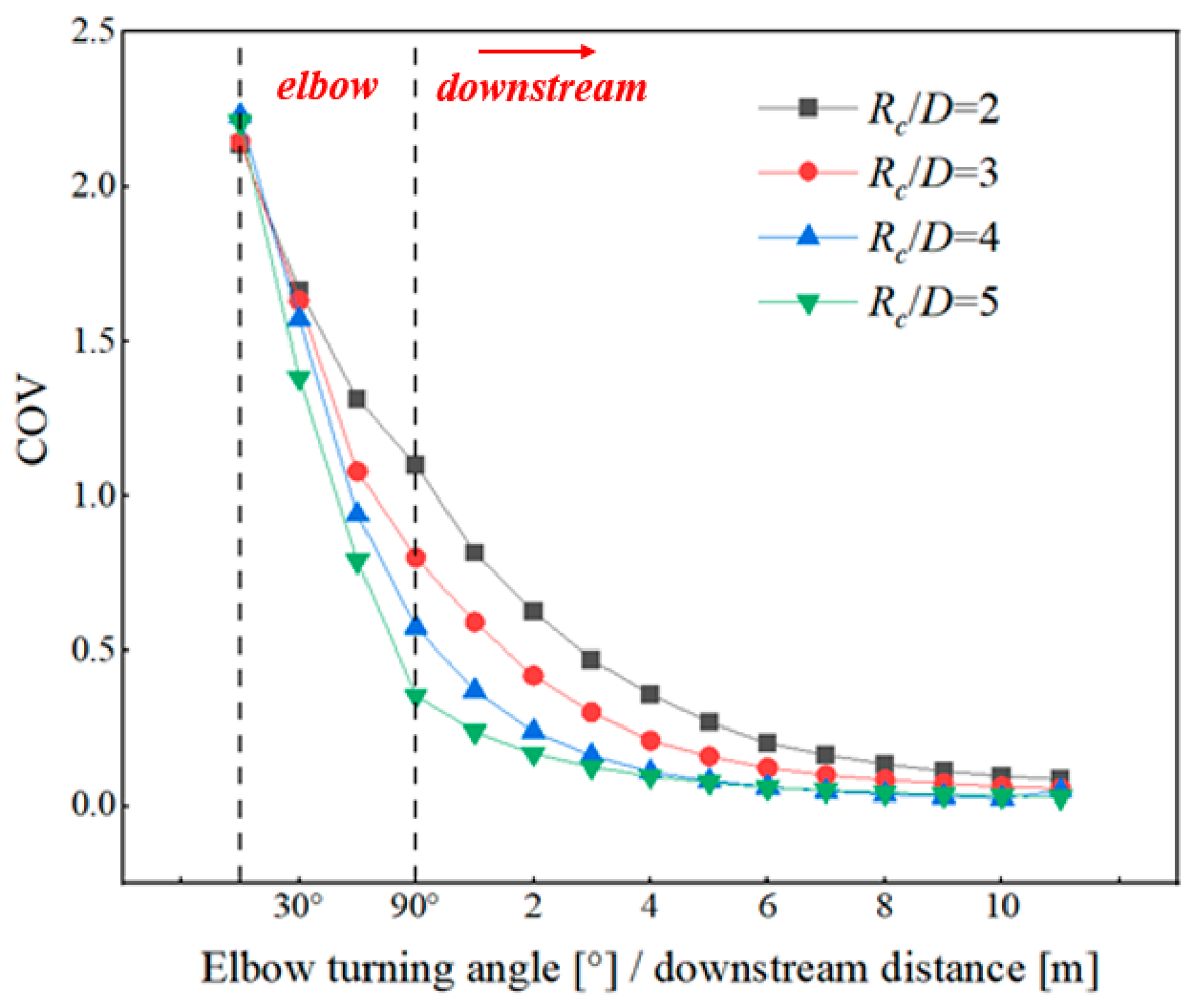
Figure 15 illustrates the distribution of hydrogen molar fraction in elbow pipes with different curvature radii, providing a visual representation of hydrogen distribution across various cross-sections within the pipeline. Figure 16 compares the evolution of COV within the elbow and in the downstream straight section. Because the elbow arc length varies with R_c/D, the in-elbow results are presented against the turning angle, whereas the downstream results are presented against the distance from the elbow outlet. The two regions are displayed consecutively in Figure 16 to preserve the continuity of the COV evolution and to distinguish the contribution of the elbow section from the subsequent downstream mixing process. Within the elbow, smaller R_c/D produces a greater COV reduction rate, consistent with stronger curvature-induced secondary motion. However, the overall homogeneous mixing path is not determined by the in-elbow COV decay alone, because the downstream evolution and decay of the secondary vortices also affect hydrogen redistribution.

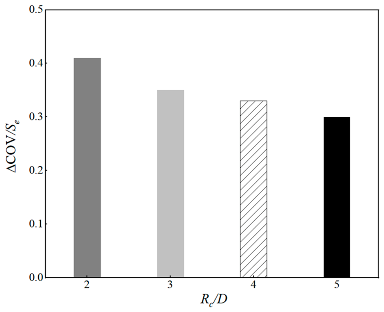
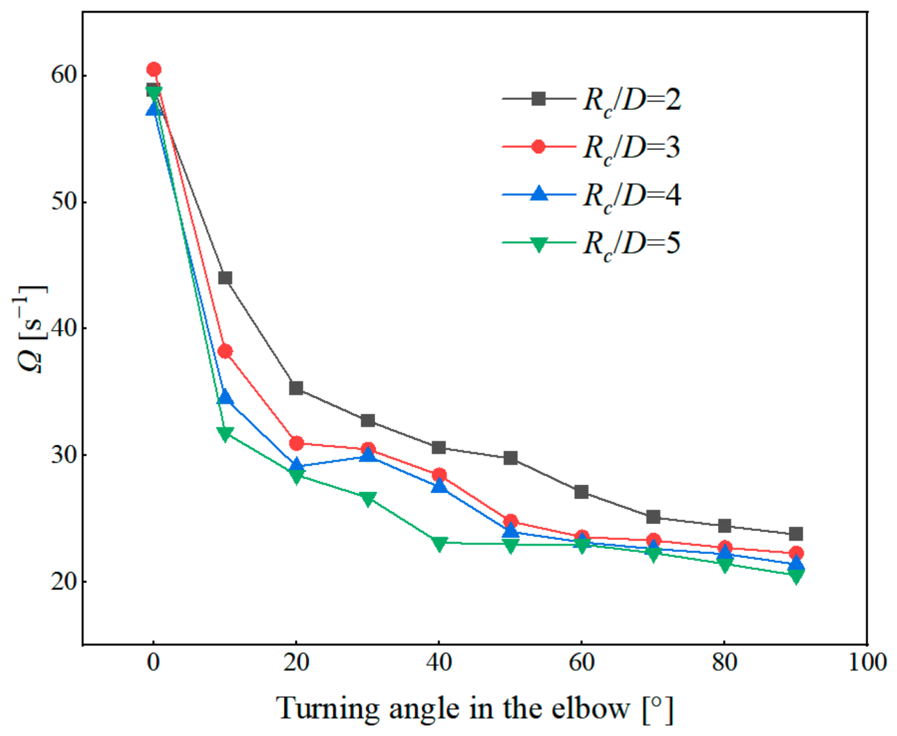
To quantify the decay of concentration non-uniformity within the elbow, ΔCOV/S_e is introduced as an evaluation metric, where ΔCOV denotes the change at the start and end of the elbow section, and S_e represents the flow path in the corresponding elbow section. Figure 17 shows that ΔCOV/S_e decreases as R_c/D increases. Figure 18 further shows that the cross-sectional average vorticity is highest at R_c/D = 2 and lowest at R_c/D = 5. The consistent trends of these two parameters indicate that stronger curvature-induced secondary motion accelerates the reduction in concentration non-uniformity within the elbow.

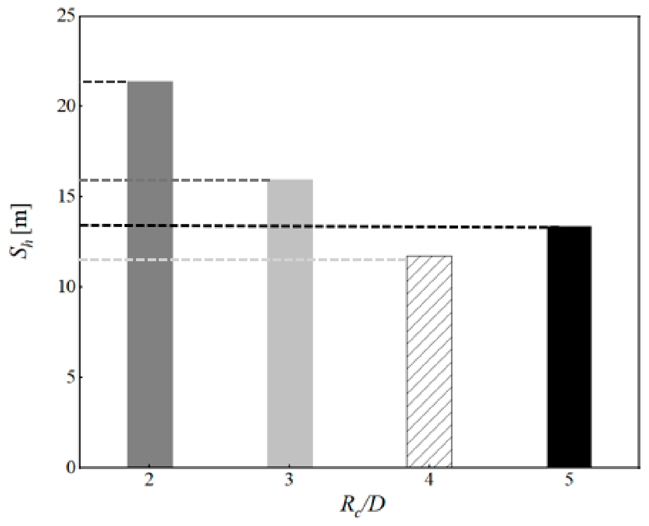
Figure 19 compares the homogeneous mixing paths for different curvature-radius ratios. The corresponding values are 21.41, 15.53, 11.73, and 13.38 m for R_c/D = 2, 3, 4, and 5, respectively. The homogeneous mixing path first decreases and then increases with R_c/D, reaching a minimum of 11.73 m at R_c/D = 4. This value is 45.21% lower than that obtained at R_c/D = 2. Although R_c/D = 2 produces the highest cross-sectional average vorticity and the greatest in-elbow COV reduction rate, it does not yield the shortest overall homogeneous mixing path. The strong centrifugal effect at R_c/D = 2 is accompanied by a pronounced asymmetric hydrogen-enrichment region, whereas the weaker secondary flow at R_c/D = 5 reduces vortex-induced transverse transport. The minimum homogeneous mixing path at R_c/D = 4 is therefore associated with sufficient secondary-flow transport, reduced concentration asymmetry, and favorable downstream vortex evolution. As R_c/D increases, the weakening centrifugal effect allows the buoyancy-driven upward migration of hydrogen to contribute more significantly to cross-sectional redistribution, which is consistent with the improved mixing reported by Eames et al. [17] for bottom hydrogen injection.

3.3. Comparison to Traditional T-Pipes

This section compares the flow structures, hydrogen distributions, COV evolutions, and homogeneous mixing paths of the conventional T-pipe and two branch–elbow configurations: L₁ = 0 m with R_c/D = 3, and L₁ = 0 m with R_c/D = 4.

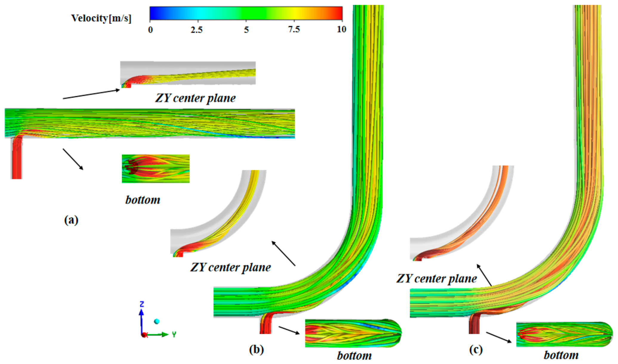
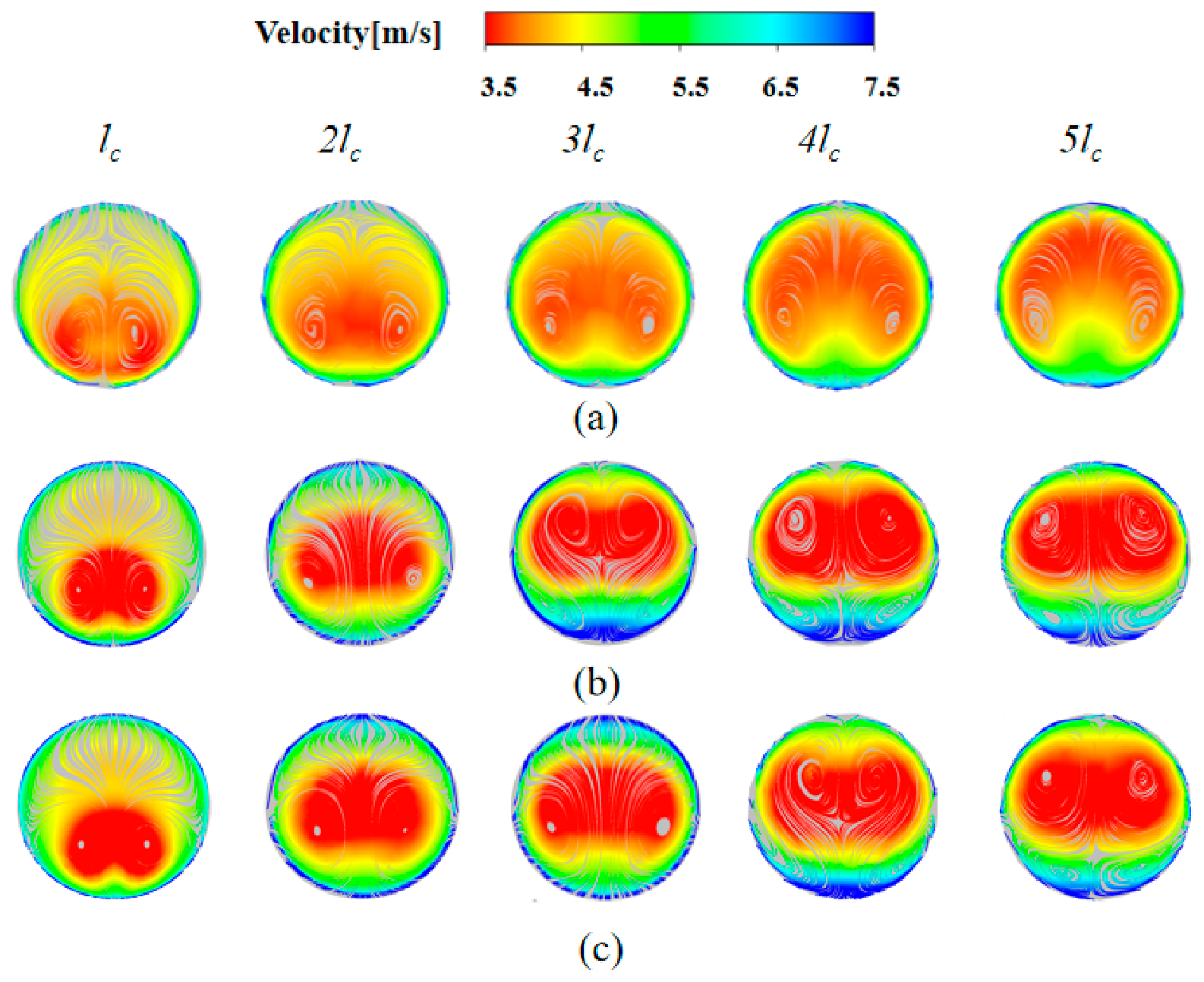
Figure 20 compares the streamlines in the three configurations. Compared with the conventional T-pipe, the branch–elbow configurations exhibit more pronounced streamline interlacing within the curved section. In Figure 20b, the stronger streamline deflection and interlacing indicate enhanced secondary-flow disturbance for the L₁ = 0 m and R_c/D = 3 configuration. The flow issuing from Inlet 2 is transported more directly toward the pipe core, whereas in the conventional T-pipe it initially remains concentrated near the lower wall before gradually moving toward the center. This difference indicates that the elbow promotes cross-sectional transport and weakens the persistence of the initial hydrogen-rich region.

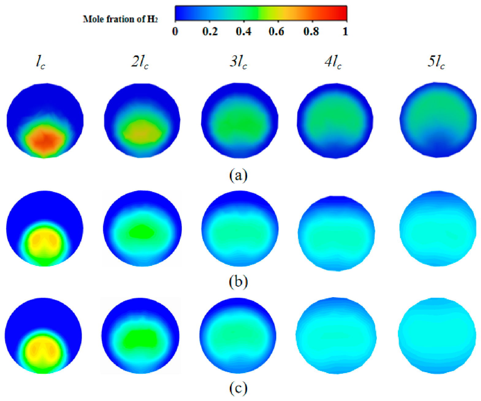
Figure 21 compares the hydrogen mole-fraction distributions at the same streamwise path length l_c. The reference length was defined as the centerline arc length from the elbow inlet to the 30° section of the L₁ = 0 m and R_c/D = 3 configuration, giving l_c ≈ 1.6D. The same path length, measured from the hydrogen injection section, was then used to determine the comparison sections in the conventional T-pipe and the R_c/D = 4 elbow. At this location, the two elbow configurations exhibit broader hydrogen distributions, lower local peak mole fractions, and more uniform cross-sectional concentration fields than the conventional T-pipe. This improvement results from curvature-induced secondary flow, which enhances transverse hydrogen transport across the pipe section.

Figure 22 compares the cross-sectional flow fields at the same centerline path length l_c. The conventional T-pipe exhibits a predominantly double-vortex structure downstream of the injection branch, whereas the branch–elbow configurations generate an additional vortex pair and a transient four-vortex structure. The subsequent merging and decay of these vortices redistribute the downstream secondary-flow field and enhance transverse species transport.

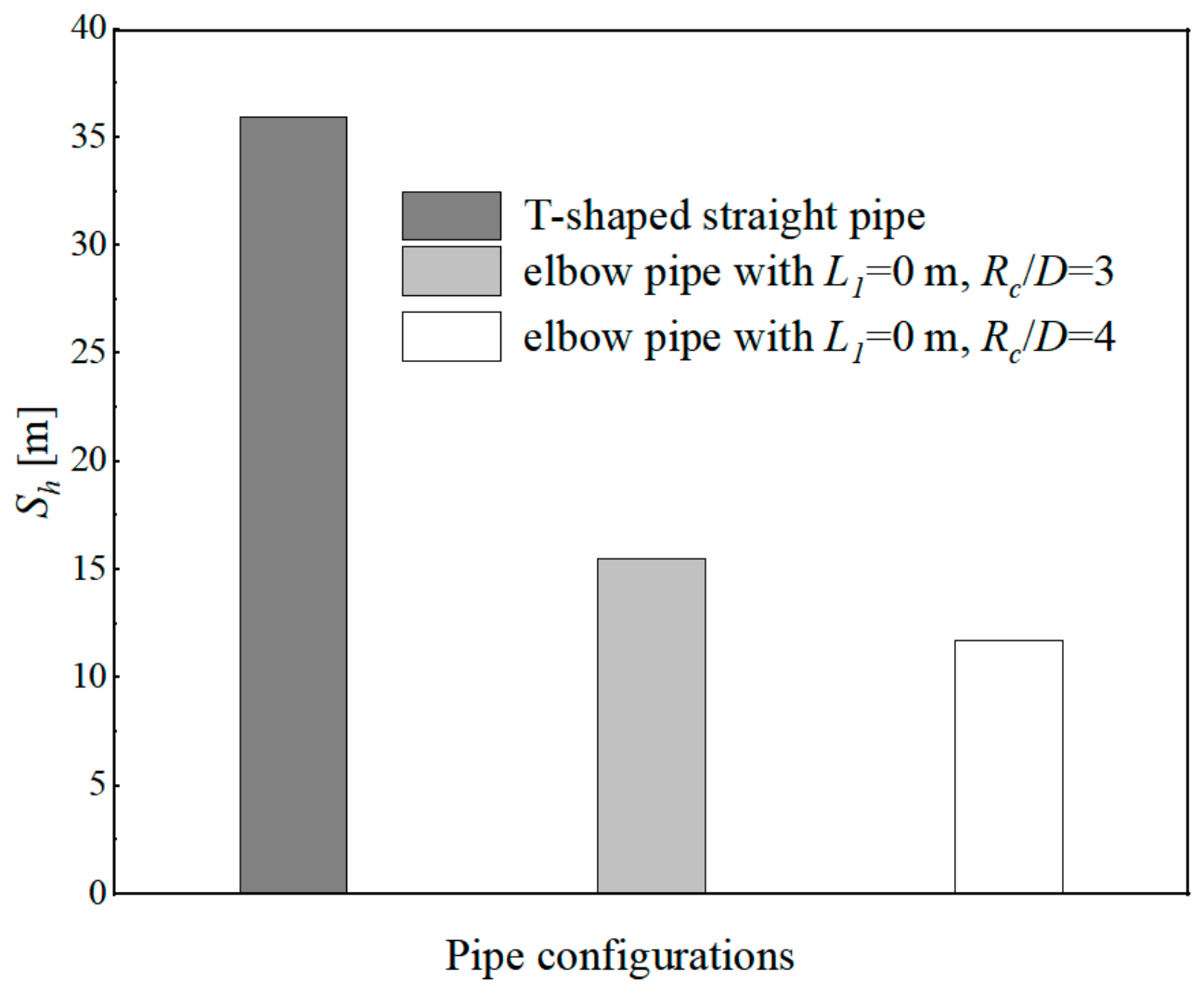
For a consistent comparison among different pipeline geometries, the hydrogen-injection section was taken as the common origin of the mixing path. The homogeneous mixing path S_h was calculated as the cumulative centerline length from the injection section to the first cross-section satisfying COV ≤ 0.05. For the conventional T-pipe, S_h corresponds to the downstream straight-pipe length, whereas for the branch–elbow configurations it includes the straight-pipe length, the elbow centerline arc length, and the downstream straight section. Thus, S_h represents the actual distance travelled by the mixed gas and provides a consistent geometric basis for comparison among the different configurations.

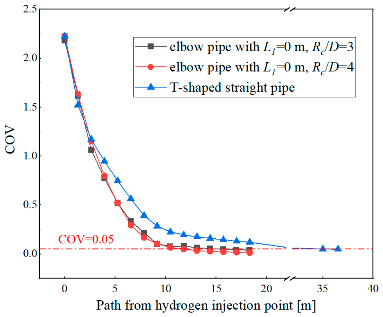
Figure 23 compares the COV evolution of the three configurations over representative downstream sections. Since the straight and branch–elbow configurations contain different geometric sections along the centerline, Figure 23 is used to illustrate the variation in concentration uniformity during the mixing process. The two branch–elbow configurations exhibit a faster reduction in COV after entering the curved section, whereas the conventional T-pipe shows a slower downstream homogenization process. The complete comparison of homogeneous mixing paths is presented separately in Figure 24 based on the centerline-defined S_h.

Figure 24 compares the homogeneous mixing paths of the conventional T-pipe and the two representative branch–elbow configurations. Relative to the conventional T-pipe, the homogeneous mixing path is reduced by 56.7% for L₁ = 0 m and R_c/D = 3, and by 67.3% for L₁ = 0 m and R_c/D = 4. These results demonstrate that the optimized branch–elbow configurations achieve more rapid hydrogen homogenization under the investigated conditions. Because the mixing enhancement is obtained using an existing pipeline component, this approach may reduce reliance on additional subsea flow-disturbing devices.

To further examine the mixing performance of the elbow configuration at different hydrogen blending ratios, additional simulations were conducted at HBRs of 15% and 20% under the same main-flow condition. As shown in

Table 3. Comparison of homogeneous mixing paths under different hydrogen blending ratios.

HBR	Sh for Elbow	Sh for T-Pipe
15%	35.81 m	40.95 m
20%	21.47 m	38.86 m
25%	11.73 m	35.90 m

, at an HBR of 15%, the homogeneous mixing paths of the elbow and conventional T-pipe are 35.81 m and 40.95 m, respectively, corresponding to a reduction of 12.55%. When the HBR increases to 20%, the corresponding homogeneous mixing paths are 21.47 m and 38.86 m, and the reduction increases to 44.75%. Together with the 67.3% reduction obtained at the original HBR of 25%, these results indicate that the elbow configuration maintains a shorter homogeneous mixing path than the conventional T-pipe over the investigated HBR range, while its relative mixing advantage becomes more pronounced with increasing HBR. In particular, under the present operating condition, the mixing enhancement provided by the elbow becomes more evident at HBRs of 20% and above.

4. Conclusions

This study investigates hydrogen-natural gas mixing in a branch–elbow configuration and clarifies the effects of the distance between the branch and elbow inlet L₁ and the elbow curvature ratio R_c/D. The elbow is utilized as a passive in-line mixing element by coupling the hydrogen jet with curvature-induced secondary flow. The main conclusions are as follows:

(1)

The effect of L₁ on the homogeneous mixing path is non-monotonic. For R_c/D = 3, a shorter L₁ allows the injected hydrogen to enter the elbow before excessive upstream flow development, thereby strengthening its interaction with the elbow-induced secondary flow and promoting transverse transport. Although the mixing path does not vary monotonically over the entire L₁ range, locating the hydrogen injection branch close to the elbow provides favorable mixing behavior under the investigated conditions. This highlights the importance of the relative position between the hydrogen injection point and the downstream elbow in pipeline layout design.

(2)

A smaller R_c/D generates stronger curvature-induced secondary flow, which enhances transverse transport and promotes hydrogen redistribution. However, the stronger centrifugal effect at small R_c/D also intensifies asymmetric hydrogen enrichment, so stronger secondary flow does not necessarily result in a shorter homogeneous mixing path. Under the investigated L₁ = 0 m configuration, the homogeneous mixing path first decreases and then increases with increasing R_c/D, reaching a minimum at R_c/D = 4. This indicates that an appropriate elbow curvature radius should be considered in pipeline layout design to balance transverse transport and concentration uniformity.

(3)

The elbow configuration maintains a shorter homogeneous mixing path than the conventional T-pipe at different hydrogen blending ratios. The reduction in homogeneous mixing path increases from 12.55% at an HBR of 15% to 44.75% at 20%, and reaches 67.3% at 25%. This indicates that the relative mixing enhancement provided by the elbow becomes more pronounced with increasing HBR, with a particularly evident advantage at HBRs of 20% and above under the investigated operating condition.

The conclusions presented in this study are applicable to the investigated hydrogen-blended natural gas pipeline conditions. Accordingly, the R_c/D = 4 configuration represents the best mixing performance among the examined cases rather than a universal optimum. Further investigations considering different hydrogen blending ratios, flow conditions, and pipeline configurations are required to establish more general design guidelines. For offshore pipeline sections with comparable operating conditions, locating the hydrogen injection branch close to an existing elbow may provide a passive approach to shorten the homogeneous mixing path without additional mixing devices.

References

1. Davis, M.; Okunlola, A.; Di Lullo, G.; Giwa, T.; Kumar, A. Greenhouse gas reduction potential and cost-effectiveness of economy-wide hydrogen-natural gas blending for energy end uses. Renew. Sustain. Energy Rev. 2023, 171, 112962. [Google Scholar] [CrossRef] [Scilit]
2. Pivetta, D.; Dall’Armi, C.; Sandrin, P.; Bogar, M.; Taccani, R. The role of hydrogen as enabler of industrial port area decarbonization. Renew. Sustain. Energy Rev. 2024, 189, 113912. [Google Scholar] [CrossRef] [Scilit]
3. Bhardwaj, K.A. Technological advancements in adopting green hydrogen in the power and energy sector. In Proceedings of the 2024 IEEE Region 10 Symposium (TENSYMP), New Delhi, India, 27–29 September 2024. [Google Scholar] [CrossRef] [Scilit]
4. Zhou, B.; Yang, Y.; Kong, Y.; Zhang, P.; Wang, T.; Lv, M.; Zhang, Z. Study on energy consumption, economy and pollutant emission of typical hydrogen production process based on life cycle assessment. In Proceedings of the 4th International Conference on Energy Engineering and Power Systems (EEPS 2024), Hangzhou, China, 9–11 August 2024; pp. 1338–1344. [Google Scholar] [CrossRef] [Scilit]
5. Panić, I.; Cuculić, A.; Ćelić, J. Color-coded hydrogen: Production and storage in maritime sector. J. Mar. Sci. Eng. 2022, 10, 1995. [Google Scholar] [CrossRef] [Scilit]
6. Taroual, K.; Nachtane, M.; Rouway, M.; Tarfaoui, M.; Faik, A.; Mînzu, V.; Hilmi, K.; Saifaoui, D. Marine renewable-driven green hydrogen production toward a sustainable solution and a low-carbon future in Morocco. J. Mar. Sci. Eng. 2024, 12, 774. [Google Scholar] [CrossRef] [Scilit]
7. Zhang, H.; Tian, Z. Failure analysis of corroded high-strength pipeline subject to hydrogen damage based on FEM and GA-BP neural network. Int. J. Hydrogen Energy 2022, 47, 4741–4758. [Google Scholar] [CrossRef] [Scilit]
8. Chen, B.-Q.; Videiro, P.M.; Guedes Soares, C. Opportunities and challenges to develop digital twins for subsea pipelines. J. Mar. Sci. Eng. 2022, 10, 739. [Google Scholar] [CrossRef] [Scilit]
9. Mariani, A.; Unich, A.; Minale, M. Combustion of hydrogen enriched methane and biogases containing hydrogen in a controlled auto-ignition engine. Appl. Sci. 2018, 8, 2667. [Google Scholar] [CrossRef] [Scilit]
10. Chen, Z.-F.; Chu, W.-P.; Wang, H.-J.; Li, Y.; Wang, W.; Meng, W.-M.; Li, Y.-X. Structural integrity assessment of hydrogen-mixed natural gas pipelines based on a new multi-parameter failure criterion. Ocean Eng. 2022, 247, 110731. [Google Scholar] [CrossRef] [Scilit]
11. Obanijesu, E.O.; Barifcani, A.; Pareek, V.K.; Tade, M.O. Experimental study on feasibility of H2 and N2 as hydrate inhibitors in natural gas pipelines. J. Chem. Eng. Data 2014, 59, 3756–3766. [Google Scholar] [CrossRef] [Scilit]
12. Liu, C.; Pei, Y.; Cui, Z.; Li, X.; Yang, H.; Xing, X.; Duan, P.; Li, L.; Li, Y. Study on the stratification of the blended gas in the pipeline with hydrogen into natural gas. Int. J. Hydrogen Energy 2023, 48, 5186–5196. [Google Scholar] [CrossRef] [Scilit]
13. Dadfarnia, M.; Sofronis, P.; Brouwer, J.; Sosa, S. Assessment of resistance to fatigue crack growth of natural gas line pipe steels carrying gas mixed with hydrogen. Int. J. Hydrogen Energy 2019, 44, 10808–10822. [Google Scholar] [CrossRef] [Scilit]
14. Wei, H.; Duan, B.; Shi, X.; Gao, R.; Hua, Z.; Qiu, S.; Zhao, Y. Influence of hydrogen in natural gas mixed hydrogen environment on mechanical properties of X80 pipeline steel. Int. J. Hydrogen Energy 2024, 54, 908–921. [Google Scholar] [CrossRef] [Scilit]
15. Du, F.; Li, C.; Wang, W. Development of subsea pipeline buckling, corrosion and leakage monitoring. J. Mar. Sci. Eng. 2023, 11, 188. [Google Scholar] [CrossRef] [Scilit]
16. Meniconi, S.; Brunone, B.; Tirello, L.; Rubin, A.; Cifrodelli, M.; Capponi, C. Transient tests for checking the Trieste subsea pipeline: Toward field tests. J. Mar. Sci. Eng. 2024, 12, 374. [Google Scholar] [CrossRef] [Scilit]
17. Eames, I.; Austin, M.; Wojcik, A. Injection of gaseous hydrogen into a natural gas pipeline. Int. J. Hydrogen Energy 2022, 47, 25745–25754. [Google Scholar] [CrossRef] [Scilit]
18. Umuteme, O.M. Computational fluid dynamics (CFD) transient pressure and temperature simulation of a natural gas–hydrogen gas blend transportation pipeline. Int. J. Innov. Res. Dev. 2020, 9, 112–116. [Google Scholar] [CrossRef] [Scilit]
19. Villuendas, T.; Montañés, C.; Gómez, A.; Alarcón, A.C.; Storch de Gracia, M.D.; Sánchez-Laínez, J. Advancing in the decarbonized future of natural gas transmission networks through a CFD study. Int. J. Hydrogen Energy 2022, 47, 15832–15844. [Google Scholar] [CrossRef] [Scilit]
20. Kuczyński, S.; Łaciak, M.; Olijnyk, A.; Szurlej, A.; Włodek, T. Thermodynamic and technical issues of hydrogen and methane-hydrogen mixtures pipeline transmission. Energies 2019, 12, 569. [Google Scholar] [CrossRef] [Scilit]
21. Yan, S.; Jia, G.; Xu, W.; Li, R.; Lu, Y.; Cai, M. Computational fluid dynamic analysis of hydrogen-injected natural gas for mixing and transportation behaviors in pipeline structures. Energy Sci. Eng. 2023, 11, 2912–2928. [Google Scholar] [CrossRef] [Scilit]
22. Han, F.; Mu, X.; Wei, Y.; Li, W.; Wang, Z. Mixing mechanisms of hydrogen-blended natural gas in subsea pipelines: Effects of injection angles. Ocean Eng. 2025, 330, 121245. [Google Scholar] [CrossRef] [Scilit]
23. Tan, K.; Mahajan, D.; Venkatesh, T.A. Computational fluid dynamic modeling of methane-hydrogen mixture transportation in pipelines: Understanding the effects of pipe roughness, pipe diameter and pipe bends. Int. J. Hydrogen Energy 2024, 49, 1028–1042. [Google Scholar] [CrossRef] [Scilit]
24. Han, F.; Liu, Y.; Lan, Q.; Li, W.; Wang, Z. CFD investigation on secondary flow characteristics in double-curved subsea pipelines with different spatial structures. J. Mar. Sci. Eng. 2022, 10, 1264. [Google Scholar] [CrossRef] [Scilit]
25. Kükrer, E.; Eskin, N. Experimental assessment of local void fraction and flow development in a U-bend piping system for air-water two-phase flow. Int. J. Multiph. Flow 2023, 169, 104610. [Google Scholar] [CrossRef] [Scilit]
26. Han, F.; Lan, Q.; Ong, M.C.; Yin, G.; Li, W. Experimental investigation on transition mechanisms and modal decomposition analysis of gas–liquid flow patterns in horizontal–vertical elbow. Phys. Fluids 2024, 36, 127156. [Google Scholar] [CrossRef] [Scilit]
27. Han, F.; Lan, Q.; Liu, Y.; Yin, G.; Ong, M.C.; Li, W.; Wang, Z. Unveiling turbulent flow dynamics in blind-tee pipelines: Enhancing fluid mixing in subsea pipeline systems. J. Mar. Sci. Eng. 2024, 12, 1199. [Google Scholar] [CrossRef] [Scilit]
28. Lee, D.; Lo, P.-H. On the enhancement of mixing in tangentially crossing micro-channels. Chem. Eng. J. 2012, 181, 524–529. [Google Scholar] [CrossRef] [Scilit]
29. Shan, Z.-H.; Zhao, Y.-G.; Pu, Y.; Sun, H.; Shi, W.-L.; Li, X.-B. Assessment of turbulence models on numerical simulation of mixing flows in T-pipe junction with upstream elbow. At. Energy Sci. Technol. 2013, 47, 1729–1734. [Google Scholar] [CrossRef]
30. Zheng, M.G.; Zeng, X.Y.; Chi, Z.H.; Sun, G.G.; Zhang, G.X.; Wang, J.Q. Numerical simulations of the mixing uniformity of tracer gas and air in 90 degree elbow duct. Adv. Mater. Res. 2011, 347, 3207–3210. [Google Scholar] [CrossRef] [Scilit]
31. Tunstall, R.; Laurence, D.; Prosser, R.; Skillen, A. Large eddy simulation of a T-Junction with upstream elbow: The role of Dean vortices in thermal fatigue. Appl. Therm. Eng. 2016, 107, 672–680. [Google Scholar] [CrossRef] [Scilit]
32. Zhou, M.; Costa Garrido, O.; Ma, S.; Zhang, N. Numerical investigation of turbulent thermal stratification at a horizontally oriented 90° pipe-elbow with varied elbow radii. Int. J. Therm. Sci. 2023, 185, 108092. [Google Scholar] [CrossRef] [Scilit]
33. Fernandes, L.A.; Marcon, L.R.C.; Rouboa, A. Simulation of flow conditions for natural gas and hydrogen blends in the distribution natural gas network. Int. J. Hydrogen Energy 2024, 59, 199–213. [Google Scholar] [CrossRef] [Scilit]
34. Gardel, A. Pressure drops in flows through T-shaped fittings. Bull. Tech. Suisse Rom. 1957, 83, 123–130. [Google Scholar]
35. Tian, Y.; Tian, T.; Ren, G.; Zhang, J. Numerical simulation of hydrogen mixing process in T-junction natural gas pipeline. Materials 2025, 18, 1879. [Google Scholar] [CrossRef] [Scilit] [PubMed]
36. Zhang, Y.; Qin, C.; Xing, H.; Liu, P. Experimental research on performance response of domestic gas cookers to variable natural gas constituents. J. Nat. Gas Sci. Eng. 2013, 10, 41–50. [Google Scholar] [CrossRef] [Scilit]
37. Shirvill, L.C.; Roberts, T.A.; Royle, M.; Willoughby, D.B.; Sathiah, P. Experimental study of hydrogen explosion in repeated pipe congestion—Part 2: Effects of increase in hydrogen concentration in hydrogen-methane-air mixture. Int. J. Hydrogen Energy 2019, 44, 3264–3276. [Google Scholar] [CrossRef] [Scilit]
38. Li, J.; Su, Y.; Yu, B.; Wang, P.; Sun, D. Influences of hydrogen blending on the Joule–Thomson coefficient of natural gas. ACS Omega 2021, 6, 16722–16735. [Google Scholar] [CrossRef] [Scilit] [PubMed]
Figure 1. Schematic diagram of the physical model.
Jmse 14 01622 g001
Figure 2. Details of the computational grids.
Jmse 14 01622 g002
Figure 3. COV results of grid independence study.
Jmse 14 01622 g003
Figure 4. Validation results against previous research [33,34].
Jmse 14 01622 g004
Figure 5. Hydrogen distributions in elbow pipes under different L1: (a) L1 = 0 m; (b) L1 = 5 m; (c) L1 = 10 m; (d) L1 = 15 m.
Jmse 14 01622 g005
Figure 6. Streamlines in the elbow section under different L1: (a) L1 = 0 m; (b) L1 = 5 m; (c) L1 = 10 m; (d) L1 = 15 m.
Jmse 14 01622 g006
Figure 7. Hydrogen distributions in the elbow section under different L1: (a) L1 = 0 m; (b) L1 = 5 m; (c) L1 = 10 m; (d) L1 = 15 m.
Jmse 14 01622 g007
Figure 8. Cross-sectional flow fields downstream of the elbow under different L1: (a) L1 = 0 m; (b) L1 = 5 m; (c) L1 = 10 m; (d) L1 = 15 m.
Jmse 14 01622 g008
Figure 9. Variations of COVα along the streamwise path from the elbow inlet for different L1 configurations.
Jmse 14 01622 g009
Figure 10. Variations in cross-sectional average vorticities in the elbow section under different L1.
Jmse 14 01622 g010
Figure 11. Comparison of homogeneous mixing paths under different L1.
Jmse 14 01622 g011
Figure 12. Hydrogen distributions in elbow pipes with different curvature radii: (a) Rc/D = 2; (b) Rc/D = 3; (c) Rc/D = 4; (d) Rc/D = 5.
Jmse 14 01622 g012
Figure 13. Streamlines in elbow sections with different curvature radii: (a) Rc/D = 2; (b) Rc/D = 3; (c) Rc/D = 4; (d) Rc/D = 5.
Jmse 14 01622 g013
Figure 14. Cross-sectional flow fields downstream of elbows with different curvature radii: (a) Rc/D = 2; (b) Rc/D = 3; (c) Rc/D = 4; (d) Rc/D = 5.
Jmse 14 01622 g014
Figure 15. Cross-sectinal hydrogen distributions along elbow pipes with different curvature radii: (a) Rc/D = 2; (b) Rc/D = 3; (c) Rc/D = 4; (d) Rc/D = 5.
Jmse 14 01622 g015
Figure 16. COV evolution through the elbow and downstream section for different Rc/D.
Jmse 14 01622 g016
Figure 17. Mean COV reduction rates within elbows with different curvature-radius ratios.
Jmse 14 01622 g017
Figure 18. Variations in cross-sectional average vorticity within elbows with different curvature-radius ratios.
Jmse 14 01622 g018
Figure 19. Comparison of homogeneous mixing paths for different curvature-radius ratios.
Jmse 14 01622 g019
Figure 20. Comparisons of streamlines in different configurations: (a) T-shaped straight pipe; (b) elbow pipe with L1 = 0 m, Rc/D = 3; (c) elbow pipe with L1 = 0 m, Rc/D = 4.
Jmse 14 01622 g020
Figure 21. Hydrogen distributions downstream in different configurations: (a) T-shaped straight pipe; (b) elbow pipe with L1 = 0 m, Rc/D = 3; (c) elbow pipe with L1 = 0 m, Rc/D = 4.
Jmse 14 01622 g021
Figure 22. Cross-sectional flow fields in different configurations: (a) T-shaped straight pipe; (b) elbow pipe with L1 = 0 m, Rc/D = 3; (c) elbow pipe with L1 = 0 m, Rc/D = 4.
Jmse 14 01622 g022
Figure 23. Comparison of COV evolution over representative downstream sections for different pipe configurations.
Jmse 14 01622 g023
Figure 24. Comparison of homogeneous mixing paths among different pipe configurations.
Jmse 14 01622 g024