A Data-Driven Matching Error Compensation Framework for Underwater Gravity Aided Inertial Navigation

Abstract

Continuity and reliability are critical for underwater gravity aided inertial navigation, while variations in gravity field suitability, sensor noise, and environmental disturbances can degrade gravity matching and navigation performance. To address this issue, a data-driven matching error compensation framework is proposed for gravity aided inertial navigation. Within this framework, a Hampel filter identifies unreliable gravity matching outputs based on local temporal consistency, and a CNN–BiLSTM–Attention model predicts compensated position increments for the flagged updates. The model maps INS position increments and measured gravity anomaly sequences to reliable gravity matching increments through local feature extraction, temporal modeling, and attention-based weighting, with offline training and online deployment. Reliable training samples were selected offline using reference trajectories, with synchronized GNSS positions serving only as the reference for sample screening in the marine experiments. Experiments were conducted across five simulated gravity field regions with five gravity matching algorithms and along three measured trajectories acquired using two types of marine gravimeters. In the marine experiments, the proposed method achieved mean APE-O values of 1.60, 1.06, and 1.06 n miles on L6, L7, and L8, respectively. The improvement was most evident on L6 with relatively extended error intervals, while the conventional RBIM method achieved comparable performance on the more regular and localized L8 error interval. Across the evaluated datasets, the proposed framework provided effective compensation for degraded gravity matching updates and improved the continuity of position corrections.

1. Introduction

Reliable long-duration positioning remains an important requirement for submerged vehicles, particularly when external navigation updates are intermittent or unavailable [1,2]. Inertial navigation systems (INS) provide continuous self-contained navigation, although positioning errors may accumulate over extended operation [3,4,5]. Gravity aided inertial navigation (GAIN) can mitigate this drift by correlating onboard gravity measurements and INS-indicated positions with a reference gravity map, providing a passive navigation aid without external signal exchange [6,7,8].

Gravity matching methods generally include correlation-based methods, such as Terrain Contour Matching (TERCOM) and Iterative Closest Contour Point (ICCP) [9,10]; probabilistic filtering approaches, such as the Sandia Inertial Terrain-Aided Navigation Algorithm (SITAN) and particle filters [11,12,13]; and learning-based or heuristic methods that exploit gravity field features and nonlinear mappings [14]. Recent developments for improved matching accuracy and robustness [15,16] include multiscale Hadamard transform differential matching [17], comprehensive feature matching [18], alternating line small-domain matching [19], robust and outlier-resistant filtering [20,21,22], and adaptive filtering based on satellite-derived gravity anomaly characteristics [23]. These studies improve matching performance and reduce the influence of abnormal measurements. However, the joint problem of detecting outliers in gravity matching position outputs and compensating the affected updates has received limited attention.

In parallel with these developments, quantitative and data-driven methods have been applied to broader maritime problems, including ship-braking modeling in ice channels [24], spatiotemporal analysis of ship carbon emissions and evaluation of low-carbon shipping pathways [25], and knowledge-graph-assisted ship-speed forecasting in ports [26]. Within underwater navigation, machine learning has been applied to geophysical field-based navigation [27], underwater simultaneous localization and mapping (SLAM), and autonomous underwater vehicle navigation [28,29,30]. These studies demonstrate the ability of data-driven models to characterize nonlinear spatial and temporal relationships, but they do not directly address outlier detection in gravity matching outputs or error compensation for unreliable position updates.

In operational GAIN, sensor noise, weak or ambiguous gravity field features, trajectory-dependent observability, reference map errors, and environmental disturbances may cause gravity matching position updates to contain gross errors or become intermittent. Feeding unreliable matching results back to the INS may introduce erroneous position corrections, whereas simply rejecting them increases the interval between valid updates and reduces navigation continuity. Reliable use of gravity matching information therefore requires both the detection of outliers in matching position outputs and the compensation of the affected updates.

Abnormal-error handling has been investigated in different navigation systems. Residual-based fault detection and exclusion, initially developed for Safety-of-Life satellite navigation, identifies inconsistent observations through residual testing and consistency checks [31,32,33]. Multi-source positioning, navigation, and timing systems further exploit redundancy among INS, GNSS, long baseline (LBL), and ultra-short baseline (USBL) measurements to cross-check unreliable observations [34]. Learning-enhanced INS/DVL fusion methods estimate uncertain measurements from sensor histories [35], while Bidirectional long short-term memory (BiLSTM) and transformer-based models capture nonlinear and time-correlated inertial navigation errors [36]. Data-driven outlier detection [37], adaptive random-error modeling [38], and sequential state-domain consistency checking [39] provide alternative means of identifying or suppressing abnormal navigation observations. Learning-based position error correction has also been investigated for underwater dead-reckoning navigation [40].

Existing studies improve navigation robustness through abnormal-observation rejection, robust weighting, measurement prediction, or data-driven error correction. In GAIN, robust filters mainly reduce the influence of abnormal measurements during state estimation, whereas learning-based methods have largely been applied to measurement prediction or navigation error correction in INS-based multisensor systems. By comparison, less attention has been paid to outliers in the position increments produced by gravity matching itself, particularly methods that first identify unreliable matching increments and then compensate for the affected position updates using INS motion information and measured gravity anomaly sequences.

To address this problem, this paper proposes a data-driven matching error compensation framework for underwater GAIN. A Hampel-filter-based confidence analysis first monitors gravity matching position increments and identifies outputs containing gross errors. A convolutional neural network–bidirectional long short-term memory-attention (CNN–BiLSTM–Attention) predictor then maps INS position increments and gravity anomaly sequences to reliable gravity matching position increments through local feature extraction, bidirectional temporal modeling, and adaptive weighting. The model is trained offline and executed online after the prescribed input sequence becomes available. When a matching output is identified as unreliable, the predicted increment is used to compensate for the affected position update, thereby maintaining the continuity of gravity matching corrections.

The main contributions of this work are summarized as follows:

•

A gravity matching outlier detection and error compensation framework is developed by combining Hampel-filter-based confidence analysis with learned position-increment prediction. Unlike methods that only reject or down-weight abnormal observations, the proposed framework provides a compensated increment for an unreliable matching update.

•

A CNN–BiLSTM–Attention predictor is constructed to learn the relationship between INS position increments, gravity anomaly sequences, and reliable gravity matching position increments. The network integrates local feature extraction, bidirectional temporal modeling, and adaptive weighting and supports offline training and window-based online inference.

•

The framework is evaluated in five simulated gravity field regions using five gravity matching algorithms and on three measured trajectories acquired using two types of marine gravimeters. The average position error in outlier segments (APE-O), matching success rate in outlier segments (MSR-O), outlier recall rate (Recall-O), and average position error over the entire trajectory (APE-T) are used to evaluate outlier error detection and compensation performance.

The remainder of this paper is organized as follows. Section 2 introduces the principles of gravity aided inertial navigation and presents the proposed CNN–BiLSTM–Attention-based matching error compensation framework. Section 3 describes the experimental setup and evaluates the proposed framework using simulated and measured marine gravity data. Section 4 discusses the experimental findings, practical implications, and limitations of the current study. Finally, Section 5 summarizes the main conclusions and outlines directions for future work.

2. Gravity Matching Outlier Detection and Error Compensation Method

2.1. GAIN System

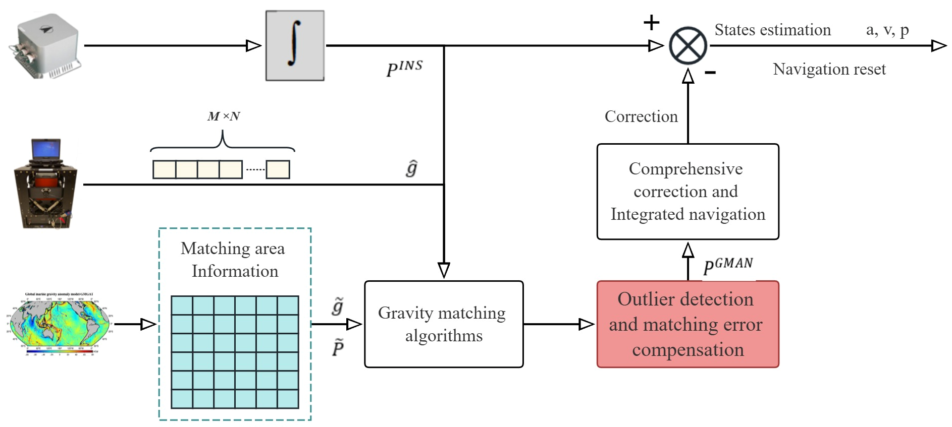
A gravity aided inertial navigation system (GAIN) typically comprises an inertial navigation system (INS), a gravity reference map, a marine gravimeter, and a high-precision, robust, and operational gravity matching–aided navigation (GMAN) algorithm. The fundamental working principle of GAIN is illustrated in Figure 1.

Gravity matching can be conceptualized as a one-dimensional correlation analysis problem, as gravimeters typically perform point-by-point measurements along the survey line. In practice, however, the matching process operates on a two-dimensional gravity reference map defined by horizontal position and anomaly values. As a result, the gravity measurements and the INS-derived position increments are combined to form a gravity measurement pattern. This pattern embeds both the spatial evolution of the trajectory and the numerical variations in the anomaly field, thereby retaining the spatially meaningful information along the navigation trajectory that is critical for reliable correlation [17,18].

$$P_k=[P_k^{INS},g_k]$$

(1)

Here, $P_k^{INS}$ is the INS position, $g_k$ is gravity measurement data, $P_k$ is a gravity measurement pattern. Generally, this correlation-based matching process can be expressed as [18]:

$$Ref(P_k,B)=COR{(P_k,B)}_{\max }$$

(2)

Here, $B={\left\{B_j\right\}}_{j=1}^{N_c}$ denotes the set of candidate gravity reference sequences extracted from the search region, and $N_c$ is the number of candidate sequences. The function $COR(P_k,B_j)$ evaluates the similarity between the measured gravity pattern $P_k$ and each candidate sequence $B_j$, and the candidate yielding the highest scalar correlation score is selected as the matching result. The map location associated with the selected sequence is determined as the gravity matching position.

Although the gravity reference map is defined in a two-dimensional geographical space, gravity observations are acquired sequentially along the vehicle trajectory. During gravity matching, gravity values at the candidate positions surrounding the INS-derived trajectory are extracted from the reference map and arranged in sampling order to form candidate reference sequences. These sequences are compared with the measured gravity sequence, and the candidate sequence yielding the optimal matching score determines the gravity matching position. In this representation, the candidate coordinates retain the spatial location and direction of the trajectory, while the ordered gravity values describe the along-track variation of the gravity field.

In the context of AUV navigation, once sufficient sailing distance had been covered, gravity matching was conducted by comparing gravity features with reference maps to obtain precise positional estimates. However, due to gravity measurement noise, trajectory-dependent observability, and spatial variability of gravity suitability, gravity matching position outputs are often irregular, sparse, and occasionally contaminated by isolated outliers. Removing these unreliable solutions further leads to nonuniform and discontinuous position updates.

To prevent unreliable gravity matching outputs from propagating into the INS fusion stage, an outlier detection and matching error compensation module is placed between gravity matching and integrated navigation. The Hampel filter first flags position increments that violate the local temporal consistency criterion, after which the CNN–BiLSTM–Attention model predicts compensated increments for the flagged updates before INS correction. Accordingly, the proposed method performs sample-level outlier detection and matching error compensation to reduce the influence of unreliable gravity matching updates on subsequent INS correction.

2.2. Robust Outlier Detection Using the Hampel Filter

Influenced by gravity measurement noise, variable trajectories, and dynamic changes in gravity suitability, the output positions of gravity matching contain numerous outliers. Given that underwater vehicles typically operate at a relatively constant depth and maintain near-uniform speed, the gravity matching position increments remain approximately stable under normal conditions. This property allows the Hampel filter to identify and remove outliers by monitoring deviations in these matching position increments $\Delta P_k^{GMAN}$, rather than relying on absolute matching errors.

To enhance reliability, a Hampel filter is introduced to assess the local temporal consistency of gravity matching position increments [41]. For the $k$th sample, a trailing one-sided window spanning $k-2t$ to $k$ is used to compute the local median $med(·)$ and the median absolute deviation ${\delta }_k$. In this study, $t=5$, corresponding to a total window length of $w=2t+1=11$ samples. Since the current increment is located at the end of the window, the consistency test uses only the current gravity matching increment and preceding available increments, including previously accepted or compensated increments. No future samples are required, thereby ensuring online causality. An increment exceeding the confidence threshold $\lambda \cdot {\delta }_k$ is flagged as potentially unreliable.

$$C_k=\left\{\begin{array}{cc}1,& if(\left|\Delta P_k^{GMAN}-med\left(\Delta P_{k-2t:k}^{GMAN}\right)\right|\le \lambda {\delta }_k)\\ 0,& if(\left|\Delta P_k^{GMAN}-med\left(\Delta P_{k-2t:k}^{GMAN}\right)\right|>\lambda {\delta }_k)\end{array}\right.$$

(3)

Here, $\Delta P_k^{GMAN}$ represents the gravity matching position increment at the $k$th sampling point, and $C_k$ is the confidence indicator, with $C_k=1$ denoting a locally consistent increment and $C_k=0$ denoting a potentially unreliable increment. The local median is calculated as $m_k=med(\Delta P_{k-2t:k}^{GMAN})$, and ${\delta }_k=med(|\Delta P_j^{GMAN}-m_k|)$, $j\in [k-2t,k]$, where $\lambda$ is the confidence threshold.

During offline data preparation and performance evaluation, the ground-truth matching error was defined as:

$$e_k^{GT}=\Vert P_k^{GMAN}-P_k^{GT}{\Vert }_2$$

(4)

Here, $P_k^{GMAN}$ denotes the gravity matching position and $P_k^{GT}$ denotes the corresponding ground-truth position at the $k$th sampling point. In the simulation experiments, $P_k^{GT}$ was obtained from the prescribed true trajectory, whereas in the marine experiments it was provided by the synchronized GNSS trajectory. Both positions were represented in the same local grid coordinate system, and $e_k^{GT}$ was expressed in nautical miles. Continuous samples satisfying $e_k^{GT}<2$ nautical miles were retained to construct the nominal training sequences, whereas samples satisfying $e_k^{GT}\ge 2$ nautical miles were regarded as matching outliers during offline performance evaluation. This criterion was used only to construct reference labels for offline training-sample selection and performance evaluation.

During online operation, neither $P_k^{GT}$ nor $e_k^{GT}$ is available. The Hampel identifier therefore uses only the gravity matching position increments to evaluate their local temporal consistency and flag potentially unreliable increments. The resulting confidence indicator is then used to trigger the subsequent matching error compensation.

2.3. Gravity Matching Error Compensation Model Based CNN–BiLSTM–Attention

2.3.1. CNN–BiLSTM–Attention Algorithm Structure

Following Hampel-based outlier detection, the CNN–BiLSTM–Attention model predicts a compensated gravity matching position increment for each flagged update. Gravity matching estimates position by correlating a measured gravity sequence with candidate sequences extracted from the reference map. Consistent with this sequence-based mechanism, the predictor takes a temporal window of INS position increments and measured gravity anomalies as input. The window is sufficiently long to represent local gravity anomaly variation and the associated INS motion evolution, while remaining short enough to preserve local vehicle dynamics [42].

The input to the CNN–BiLSTM–Attention model consists of two components: the position increments $\Delta P^{INS}$ from the INS position $P^{INS}$, and the gravity anomaly measurements $g$ corresponding to the current INS sampling points:

$$X_{in,k}={[x_{k-L+1}\hspace{1em}{x}_{k-L+2}\hspace{1em}\dots x_{k-3}\hspace{1em}{x}_{k-2}\hspace{1em}{x}_k]}^T, k\in {\mathsf{\Omega }}_{outlier}, k\ge L$$

(5)

$$x_k=\left[\begin{array}{cc}\begin{array}{cc}\Delta {\phi }_k^{INS}& \Delta {\lambda }_k^{INS}\end{array}& g_k\end{array}\right], \Delta P_k^{INS}=\left[\begin{array}{cc}\Delta L_k^{INS}& \Delta {\lambda }_k^{INS}\end{array}\right]$$

(6)

Here, $k$ denotes the sampling index, $\begin{array}{cc}\Delta L_k^{INS},& \Delta {\lambda }_k^{INS}\end{array}$ are the increments in the INS latitude and longitude at the $k$th sampling point, respectively. ${\mathsf{\Omega }}_{outlier}$ denotes the set of indices identified as outliers by the Hampel filter. $L$ denotes the time-window length.

The output of the error compensation model is the predicted gravity matching position increment at the $k$th sampling point.

$$Y_{out,k}=\Delta P_k^{GMAN}=\left[\begin{array}{cc}\Delta L_k^{GMAN}& \Delta {\lambda }_k^{GMAN}\end{array}\right], k\in {\mathsf{\Omega }}_{outlier}$$

(7)

Here, $\Delta P_k^{GMAN}$ is the gravity matching position increment at the $k$th sampling point. Its spatial components, $\begin{array}{cc}\Delta L_k^{GMAN},& \Delta {\lambda }_k^{GMAN}\end{array}$, denote the increments in the gravity matching latitude and longitude, respectively. By training the CNN–BiLSTM–Attention model on the inputs $\Delta P^{INS}$ and $g$, and the output $\Delta P^{GMAN}$, the mapping relationship between inputs and outputs, thereby compensating for outliers, was learned in gravity aided navigation.

2.3.2. Fundamentals of the CNN–BiLSTM–Attention Model

The CNN–BiLSTM–Attention model combines local feature extraction, temporal-dependency modeling, and attention-based feature weighting. According to (5) and (6), the input window $X_k$ contains $L$ consecutive observations, each comprising the INS latitude increment, INS longitude increment, and corresponding gravity anomaly value. These observations are arranged in sampling order to form a three-channel sequence. A one-dimensional convolution is first performed along the temporal sampling dimension to extract local joint patterns from adjacent observations [30,43]:

$$X_k=X_{in}, H_k^{CNN}=Relu(W_C\ast X_k+b_c)$$

(8)

Here, $W_C,b_C$ denote the convolution-kernel weights and bias, respectively, and ∗ represents one-dimensional convolution along the temporal sampling dimension. Each convolution kernel jointly processes adjacent INS position increments and gravity anomaly observations to characterize their local coupled variation along the trajectory. The resulting feature representation is subsequently provided to the BiLSTM layers for temporal-dependency modeling. The rectified linear unit is defined as $Relu(z)=max(0,z)$.

Based on the extracted spatial features $H_k^{CNN}$, a BiLSTM is then employed to capture bidirectional temporal dependencies [37]:

$$h_k^1=LST{M}_{fwd}(H_k^{CNN}), h_k^2=LST{M}_{bwd}(H_k^{CNN})$$

(9)

Here, $LST{M}_{fwd}$ and $LST{M}_{bwd}$ represent the forward and backward temporal dependencies, respectively. These dependencies are concatenated to form the bidirectional representation:

$$H_k^{BiLSTM}=\left[h_k^1,h_k^2\right]$$

(10)

Next, an attention mechanism is applied to adaptively assign weights and emphasize critical temporal features [36]:

$$H_k^{Attention}={\displaystyle \sum _{t=1}^L{\alpha }_{k,t}{H}_{k,t}^{BiLSTM}}$$

(11)

Here, ${\alpha }_{k,t}$ denotes the attention weight at the $t$th time step of the $k$th input window, computed by scoring $H_k^{BiLSTM}$ and applying normalization, where $t=1\dots L$.

Finally, a fully connected linear output layer is introduced after the attention module to generate the predicted compensation increment:

$$\Delta {\widehat{P}}_k^{GMAN}=W_o{H}_k^{Attention}+b_o$$

(12)

$$P_k^{correct}=P_{k-1}^{GMAN}+\Delta {\widehat{P}}_k^{GMAN}, k\in {\mathsf{\Omega }}_{outlier}$$

(13)

Here, $W_o$ and $b_o$ are the trainable weight matrix and bias vector of the output layer, respectively. The predicted increment $\Delta {\widehat{P}}_k^{GMAN}$ maps the preceding gravity matching position $P_{k-1}^{GMAN}$ to the corrected position $P_k^{correct}$. For the corresponding ground-truth position $P_k^{GT}$, the ideal increment is expressed as:

$$\Delta P_k^{*}=P_k^{GT}-P_{k-1}^{GMAN}$$

(14)

Based on Equations (13) and (14), the corrected position error satisfies:

$$\Vert P_k^{correct}-P_k^{GT}{\Vert }_2=\Vert \Delta {\widehat{P}}_k^{GMAN}-\Delta P_k^{*}{\Vert }_2$$

(15)

Thus, the deviation of the predicted compensation increment from its ideal value is directly reflected in the corrected position error.

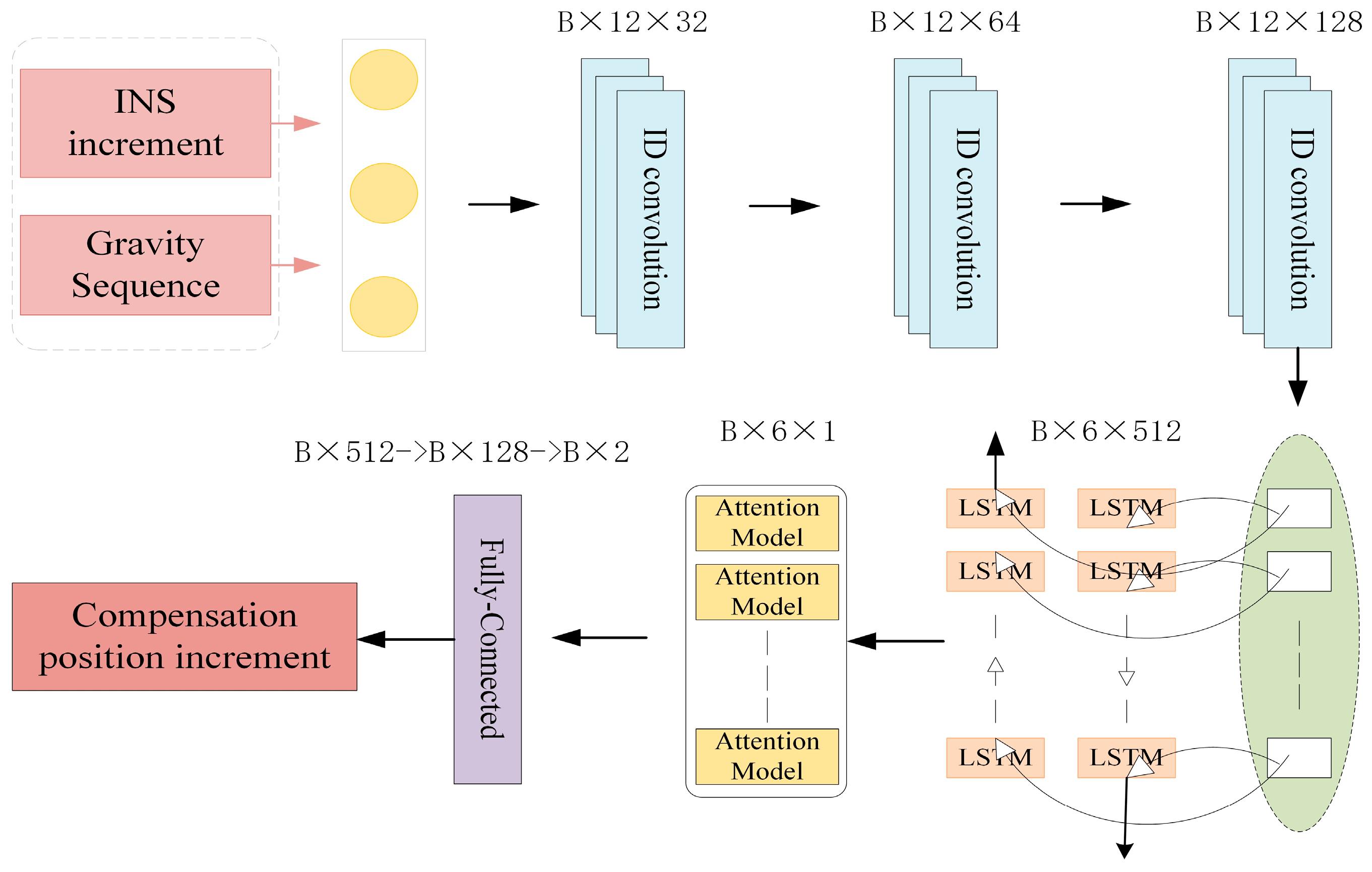
In this work, the hyperparameters are selected through a range-based tuning strategy considering regional gravity field variability and the training stability of the CNN–BiLSTM–Attention architecture. The resulting model combines spatial feature extraction, bidirectional temporal-dependency modeling, and attention-based feature weighting for position-increment prediction. The architecture is illustrated in Figure 2.

2.3.3. Outlier Detection and Matching Error Compensation Process in GAIN

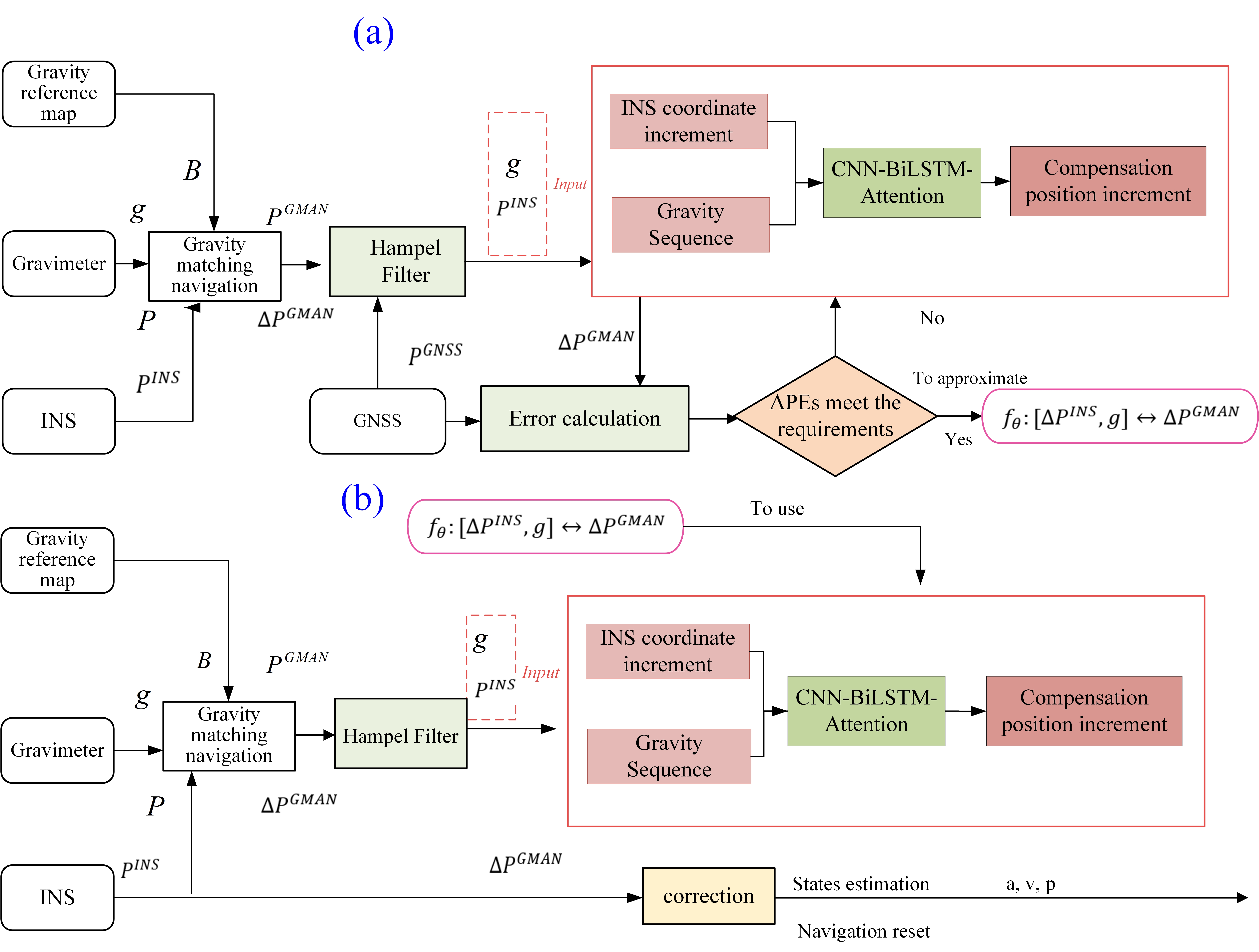
The CNN–BiLSTM–Attention model functions as an error compensation predictor for underwater gravity aided navigation. The application framework comprises two stages: a training process and a correction process, as illustrated in Figure 3.

Training process: For each trajectory and gravity matching method, an independent dataset is constructed using the corresponding INS position increments and gravity anomaly observations as inputs. The regression targets are reliable gravity matching position increments generated by the same matching method; outputs from MSD, MAD, NCC, HTD, and CFM are therefore not mixed in a common dataset. Training samples are first screened using the Hampel criterion to remove isolated anomalous increments and are further restricted to samples with ground-truth residuals below 2 nautical miles, as defined in (4). The same network architecture and training configuration are used across the evaluated matching methods, whereas the model parameters are learned independently for each trajectory-matching-method dataset. Temporal windows of INS increments and gravity anomalies are then used to learn the mapping to reliable gravity matching position increments. Training continues until the prescribed convergence criterion is satisfied.

Correction process: During deployment, the Hampel filter evaluates the local temporal consistency of each gravity matching position increment. Increments satisfying the criterion $C_k=1$ are retained, whereas those flagged as outliers $C_k=0$ are replaced by the position increments predicted by the CNN–BiLSTM–Attention model. The Hampel criterion in (3) provides a deterministic local-consistency test rather than a probabilistic confidence interval. Locally consistent increments are retained, whereas flagged increments are routed to the matching error compensation stage. For each flagged update, the CNN–BiLSTM–Attention model associated with the active gravity matching method processes a temporal window of INS position increments and measured gravity anomalies to predict a compensated gravity matching position increment. The compensated position is obtained by adding the predicted increment to the preceding available position, which may be an accepted gravity matching position or a previously compensated position, thereby maintaining the continuity of the available position updates.

2.3.4. Procedures

The complete procedures of the proposed method are summarized in Algorithm 1, with Steps 1–5 corresponding to the training stage and Step 6 to the correction stage.

Algorithm 1. Procedures of CNN–BiLSTM–Attention

Step 1. Collect GNSS, INS, and gravimeter data during AUV navigation.

Step 2. Apply gravity matching algorithm to obtain gravity matching positions.

Step 3. Construct the training dataset according to predefined criteria. Step 4. Robust confidence analysis using the Hampel Filter.

Step 5. Train the CNN–BiLSTM–Attention matching error compensation model using the screened training dataset.

Step 6. Apply the trained model in real-time to correct outliers during AUV operation.

3. Experiments and Discussion

3.1. Experimental Settings

To comprehensively evaluate the proposed gravity matching error compensation framework, a two-stage assessment strategy was implemented.

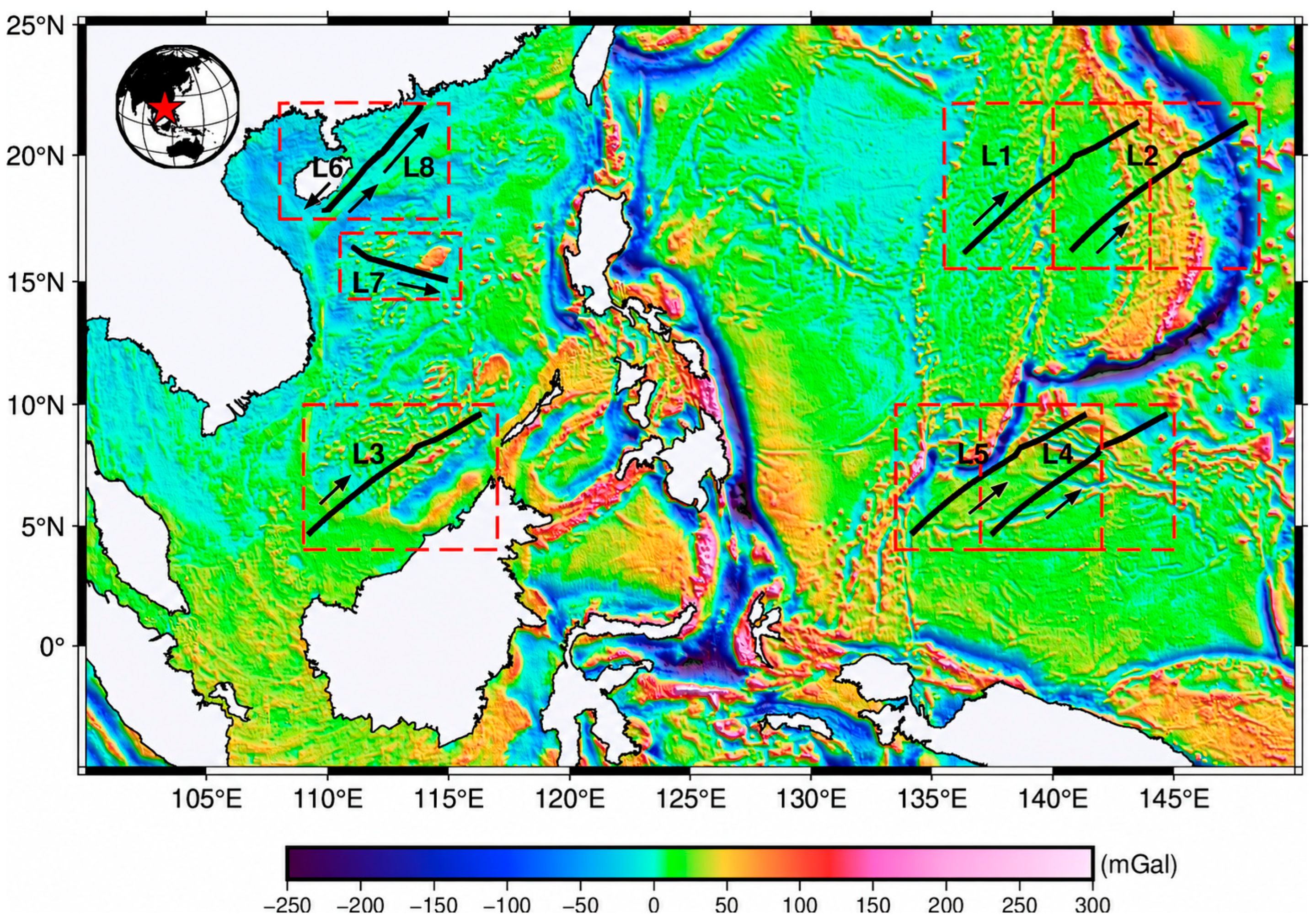
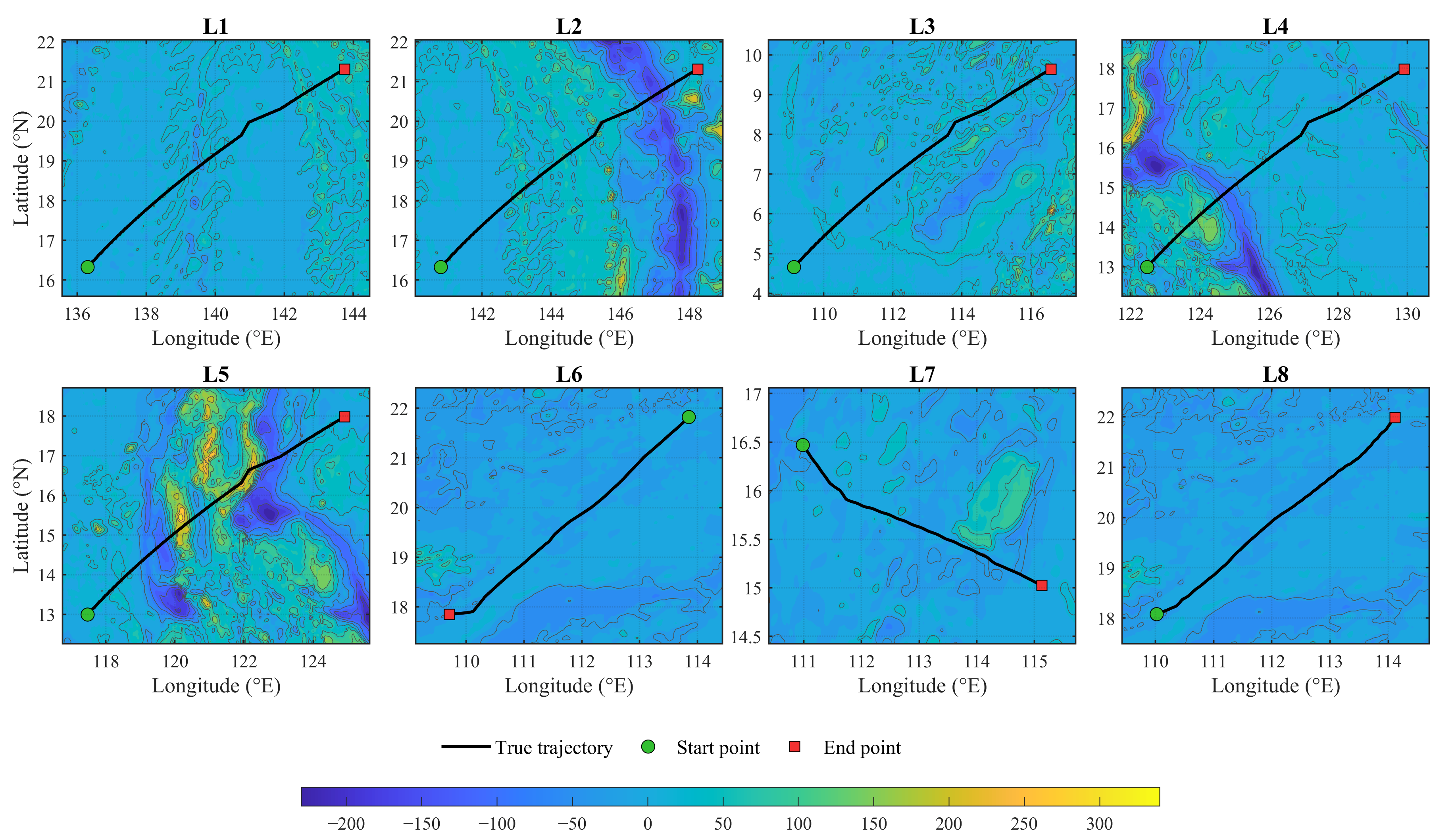
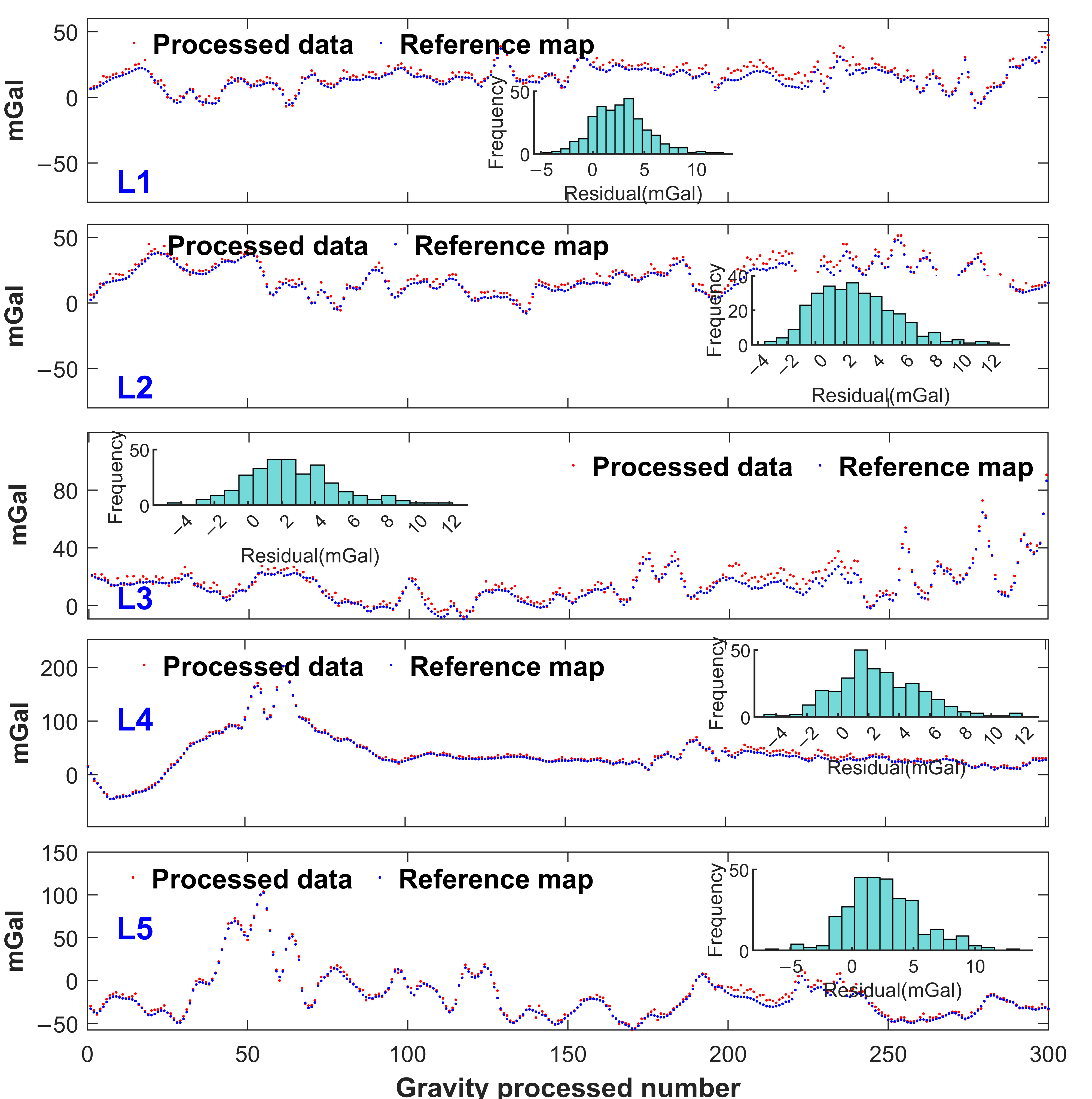
In the first stage, simulation experiments were conducted to evaluate the feasibility and applicability of the proposed method with different gravity matching algorithms, gravity field regions, and gravity measurement conditions. Five representative gravity matching algorithms, including Mean Square Deviation (MSD), Mean Absolute Deviation (MAD), Normalized Cross-Correlation (NCC), Hadamard Transform Difference (HTD), and CFM [17,18], were applied to generate position estimates. These gravity matching outputs were subsequently evaluated using the proposed CNN–BiLSTM–Attention matching error compensation framework. All simulations were performed using a gridded marine gravity database with a spatial resolution of 1′ × 1′ (1′ = 1 nautical mile = 1852 m) and an estimated accuracy of approximately 2–3 mGal [44]. Consistent with the grid-based accuracy characterization used in gravity matching navigation [17], a matching position error within two grid cells (2 n miles) was regarded as a nominal matching result. In addition, five representative trajectories (L1–L5), each 300 nautical miles long, were generated for comparison (Figure 4 and Figure 5). The simulated gravity measurements along each trajectory were corrupted by Gaussian noise $n_g~N({\mu }_g,{\sigma }_g^2)$, where ${\mu }_g$ and ${\sigma }_g^2$ denote the noise mean in mGal and variance in mGal², respectively. The baseline simulation used ${\mu }_g=2$ mGal, ${\sigma }_g^2=5$ mGal², and an INS gyroscope bias of 0.003°/h, as shown in Figure 6 and

Table 1. Survey basic information of survey lines.

Track	Grav.	Offshore Accuracy	Dis. (km)	Vel. (Kn)	Sample Freq.	Filter Length.	Process Num.
L1	Area 01	2 mGal	555.6	10	1 Hz	360 s	300
L2	Area 02	2 mGal	555.6	10	1 Hz	360 s	300
L3	Area 03	2 mGal	555.6	10	1 Hz	360 s	300
L4	Area 04	2 mGal	555.6	10	1 Hz	360 s	300
L5	Area 05	2 mGal	555.6	10	1 Hz	360 s	300
L6	KSS-31	1 mGal	630	9	1 Hz	300 s	994
L7	JMG	2 mGal	463.84	11	1 Hz	100 s	800
L8	KSS-31	1 mGal	597.08	9	1 Hz	150 s	865

. Accordingly, L1 and L2 represent relatively low-variability gravity fields, L3 represents an intermediate condition, and L4 and L5 represent comparatively high-variability gravity fields.

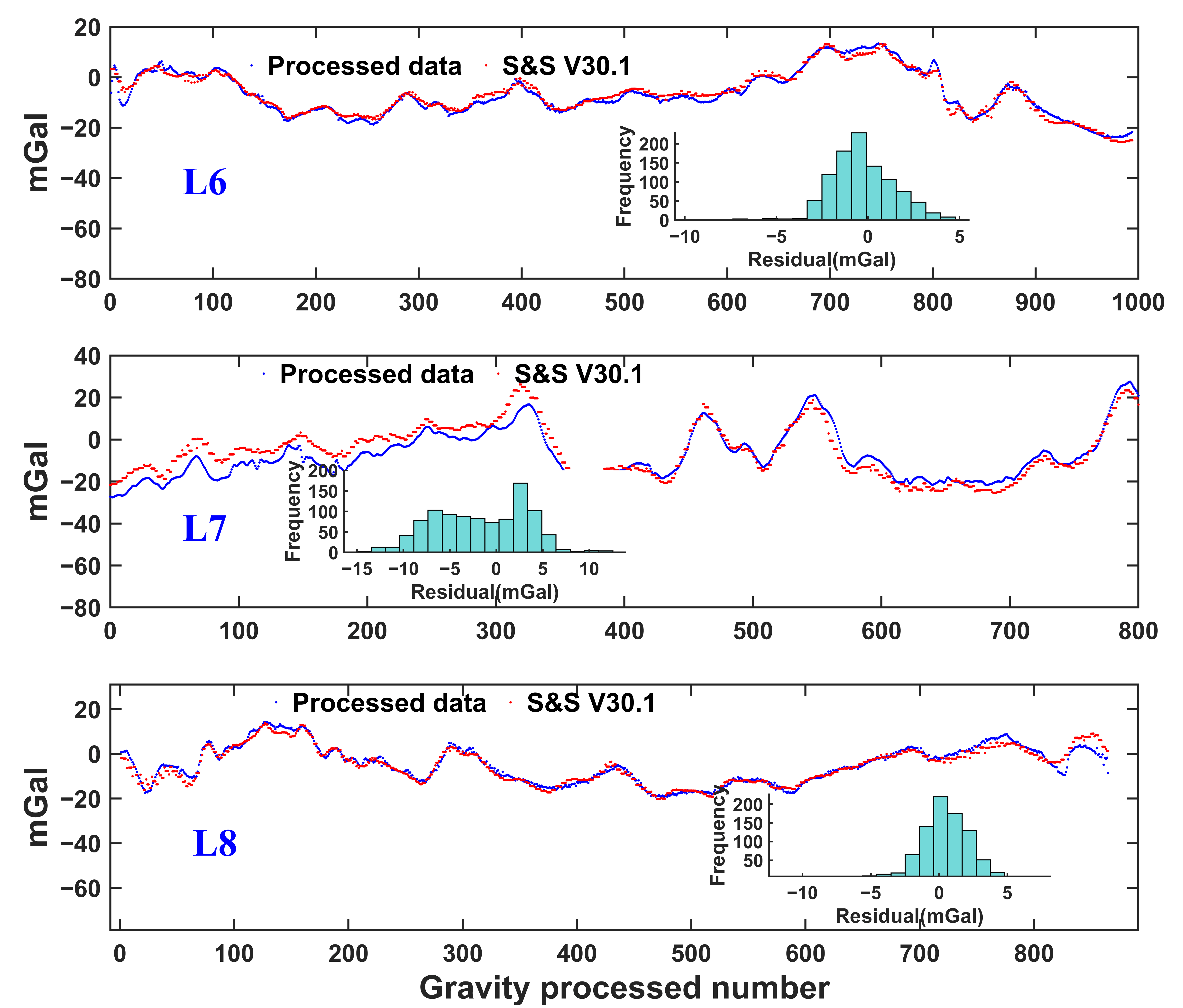
In the second stage, marine experiments were conducted to assess the robustness and practical applicability of the proposed error compensation framework under realistic measurement conditions. Three measured trajectory datasets (L6–L8) were collected in the South China Sea using two types of marine gravimeters: a KSS-31 (Bodenseewerk Geosystem GmbH, Überlingen, Germany) marine gravimeter and a self-developed JMG (Innovation Academy for Precision Measurement Science and Technology, Chinese Academy of Sciences, Wuhan, China) marine gravimeter. These instruments exhibit different noise characteristics [45]. The measured trajectories are shown in Figure 4, Figure 7 and Figure 5, with the corresponding information summarized in Table 1. To enable a comparative assessment of error compensation performance, nine representative approaches were considered, including residual-based integrity monitoring (RBIM), which reconstructs the affected matching positions by propagating the last available gravity matching position with subsequent INS-derived position increments, and least squares (LS) methods as traditional baselines [31,33]; Extended Kalman Filter (EKF), Convolutional Neural Network (CNN), long short-term memory (LSTM), and BiLSTM; CNN–BiLSTM, and more advanced attention-driven architectures, including Transformer and BiLSTM–Transformer models [36]. During the marine experiments, the INS gyro precision was 0.005°/h, and GNSS positions served as ground truth. To comprehensively assess accuracy, reliability, and computational efficiency, multiple performance metrics were evaluated for each approach.

It should be noted that the framework was applied online to the outputs of five gravity matching methods rather than used for algorithm selection, with a separate dataset and model constructed for each trajectory–method combination. Within each dataset, the preceding nominal samples were chronologically divided into 80% training and 20% validation data, while subsequent matching error intervals were reserved for testing before constructing length-12 windows; adjacent windows overlapped only within the same subset and did not cross partition boundaries. The test intervals were temporally unseen but originated from the same trajectory and gravity field region; therefore, the experiments evaluate temporal generalization under the same mission conditions.

For both stages, the Hampel filter was configured with a half-window size of $t=5$, corresponding to a total window length of $w=2t+1=11$ consecutive gravity matching outputs, and the confidence threshold was set to $\lambda =3$. The input-window length of the CNN–BiLSTM–Attention model was set to 12, with three input features at each time step. Both the input features and regression targets were normalized to the range $[0,1]$. The three convolutional layers contained 32, 64, and 128 filters with kernel sizes of 1, 3, and 5, respectively. The two stacked BiLSTM layers contained 256 and 512 hidden units, with corresponding dropout rates of 0.2 and 0.3. The dimension of the additive attention layer was set to 256, and the subsequent fully connected layer contained 128 units. The model was trained using the Adam optimizer for 200 epochs with a mini batch size of 32 and an initial learning rate of $5\times {10}^{-4}$. The learning rate was reduced by a factor of 0.8 every 100 epochs. The gradient threshold was set to 1, the samples were shuffled before each epoch, and the mean squared error was adopted as the regression loss.

Both stages adhered to identical processing principles, with the principal distinction being the source of the gravity anomaly data. Basic information on the survey is provided in Table 1. All experiments were conducted using MATLAB^® R2015b on a Dell Precision 3630 workstation equipped with a 64-bit Windows 10 operating system, an Intel^® Core™ i7-9700 CPU, and 32 GB RAM. This hardware configuration was used for both gravity matching baselines and the online inference evaluation of the proposed error compensation model.

Positioning performance was characterized using the average position error in outlier segments (APE-O), matching success rate in outlier segments (MSR-O), outlier recall rate (Recall-O), average position error over the entire trajectory (APE-T), and inference time (IT). Let ${\mathsf{\Omega }}_O$ denote the outlier sample set determined from the ground-truth trajectory using the 2-nautical-mile criterion, $N_O=\left|{\mathsf{\Omega }}_O\right|$ denote the number of outlier samples, and $N$ denote the total number of evaluated samples. The corrected position error at the $k$th sampling point is expressed as $e_k^{error}=\Vert P_k^{GMAN}-P_k^{GT}{\Vert }_2$. The corresponding metrics are:

$$APE-O={\displaystyle \frac{1}{N_O}}{\displaystyle \sum _{k\in {\mathsf{\Omega }}_O}{e}_k^{error}}$$

(16)

$$MSR-O={\displaystyle \frac{\left|\right\{k\in {\mathsf{\Omega }}_O:e_k^{error}\le 2\left\}\right|}{N_O}}\times 100\%$$

(17)

$$Recall-O={\displaystyle \frac{TP}{TP+FN}}\times 100\%$$

(18)

$$APE-T={\displaystyle \frac{1}{N}}{\displaystyle \sum _{k=1}^N{e}_k^{error}}$$

(19)

In Equations (16)–(19), APE-O describes the average corrected position error within the reference-defined outlier set ${\mathsf{\Omega }}_O$. MSR-O gives the percentage of samples in ${\mathsf{\Omega }}_O$ whose corrected position errors do not exceed 2 nautical miles, where $\left|\right\{k\in {\mathsf{\Omega }}_O:e_k^{error}\le 2\left\}\right|$ denotes the number of samples satisfying this criterion. MSR-O denotes the proportion of samples within the evaluated outlier interval whose compensated position errors satisfy the prescribed accuracy threshold. Recall-O denotes the proportion of true outlier samples, defined by original matching errors greater than 2 n miles, that are successfully recovered to within the prescribed accuracy threshold after compensation. For Recall-O, $TP$ and $FN$ denote the numbers of successfully recovered and unrecovered true outlier samples in original outliers, respectively. APE-T describes the average corrected position error over the complete trajectory, and MSR-T denotes the matching success rate over the complete trajectory, calculated as the percentage of all trajectory samples whose position errors do not exceed 2 n miles. IT is the wall-clock time consumed by the trained model during prediction on the test inputs after the Hampel screening decision becomes available; because the current gravity matching output is located at the end of the trailing window, no subsequent matching outputs are required, and the short computational time of the Hampel screening is not included in IT. Model training, gravity matching, Hampel filtering, normalization, and data preparation are not included in IT.

3.2. Simulation Experiments

The simulation experiments evaluate the robustness of the proposed framework under different gravity matching and navigation conditions by varying the gravity matching algorithm, gravity field characteristics, and measurement/navigation error conditions. Comparative evaluations with representative compensation methods are further conducted using the measured marine data.

3.2.1. Performance Across Gravity Matching Algorithms in Region L1

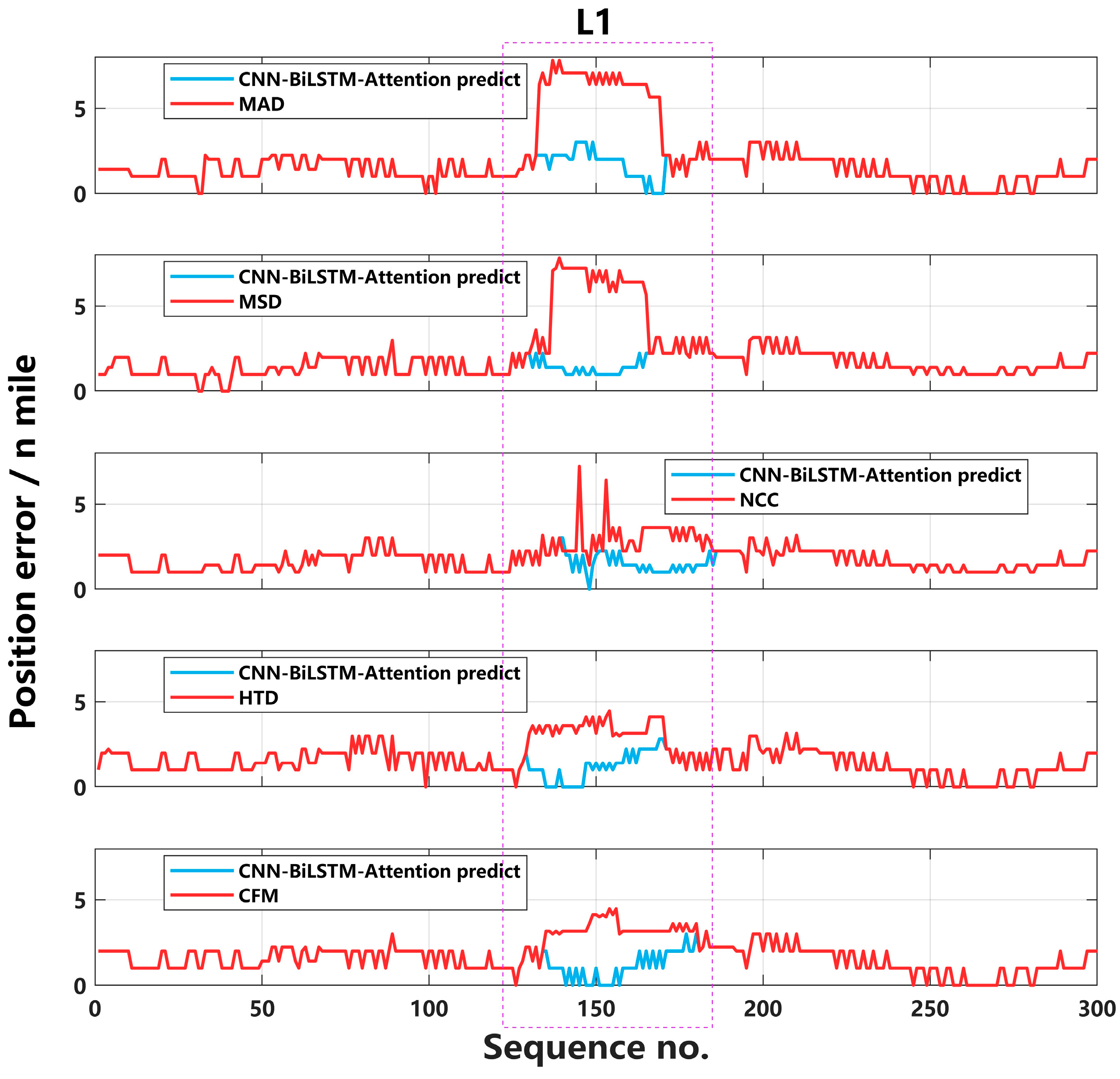
Trajectory L1 was used to evaluate the matching error compensation performance of the proposed CNN–BiLSTM–Attention model for position outputs generated by five gravity matching algorithms: MSD, MAD, NCC, HTD, and CFM. For each matching algorithm, an independent dataset was constructed from its corresponding matching outputs, and a separate CNN–BiLSTM–Attention model was trained. Data generated by different matching algorithms were not mixed, while the network architecture and hyperparameter settings remained unchanged. The original matching errors and corresponding prediction results are presented in Figure 8. Five performance indicators average position error in outlier segments (APE-O), matching success rate in outlier segments (MSR-O), outlier recall rate (Recall-O), average position error over the entire trajectory (APE-T), and inference time (IT) are summarized in

Table 2. Compensation performance of CNN–BiLSTM–Attention under different gravity matching algorithms.

Method	APE-O (n Miles)	MSR-O (%)	APE-T (n Miles)	Recall-O (%)	IT (ms)
MAD	1.72 ± 0.04	65.00 ± 1.77	1.41 ± 0.03	86.31 ± 1.72	15.51 ± 1.31
MSD	1.34 ± 0.04	87.95 ± 2.60	1.56 ± 0.05	98.48 ± 1.36	17.25 ± 1.82
NCC	1.45 ± 0.04	84.81 ± 2.09	1.62 ± 0.05	97.35 ± 1.65	15.40 ± 1.53
HTD	1.10 ± 0.03	75.26 ± 2.19	1.37 ± 0.05	94.96 ± 2.19	16.30 ± 1.57
CFM	1.10 ± 0.03	95.07 ± 2.09	1.40 ± 0.04	95.41 ± 2.07	17.86 ± 1.93

as the mean and standard deviation of five independent runs. MSR-O was calculated using the 2 nautical mile criterion defined above.

As shown in Figure 8, the original error sequences generated by the five gravity matching algorithms exhibit different amplitudes and local fluctuation patterns within the principal outlier interval. The CNN–BiLSTM–Attention model reduces the corresponding error magnitude in all five cases, although its performance varies with the characteristics of the matching output. As summarized in Table 2, HTD and CFM obtain the lowest APE-O of 1.10 ± 0.03 n miles. CFM further achieves the highest MSR-O of 95.07± 2.09%, whereas the MSR-O of HTD is 75.26 ± 2.19%, indicating that the same average error does not necessarily correspond to the same proportion of samples satisfying the 2-nautical-mile criterion. MSD and NCC achieve APE-O values of 1.34 ± 0.04 and 1.45 ± 0.04 n miles, respectively, together with Recall-O values above 97%. In comparison, the MAD output presents a more challenging error pattern, resulting in an APE-O of 1.72 ± 0.04 n miles and an MSR-O of 65.00 ± 1.77%. Across the five matching algorithms, APE-T remains between 1.37 and 1.62 n miles, while IT ranges from 15.40 to 17.86 ms. The relatively small standard deviations over five independent runs indicate stable repeatability under the different matching outputs.

3.2.2. Performance Across Gravity Field Regions Using MSD

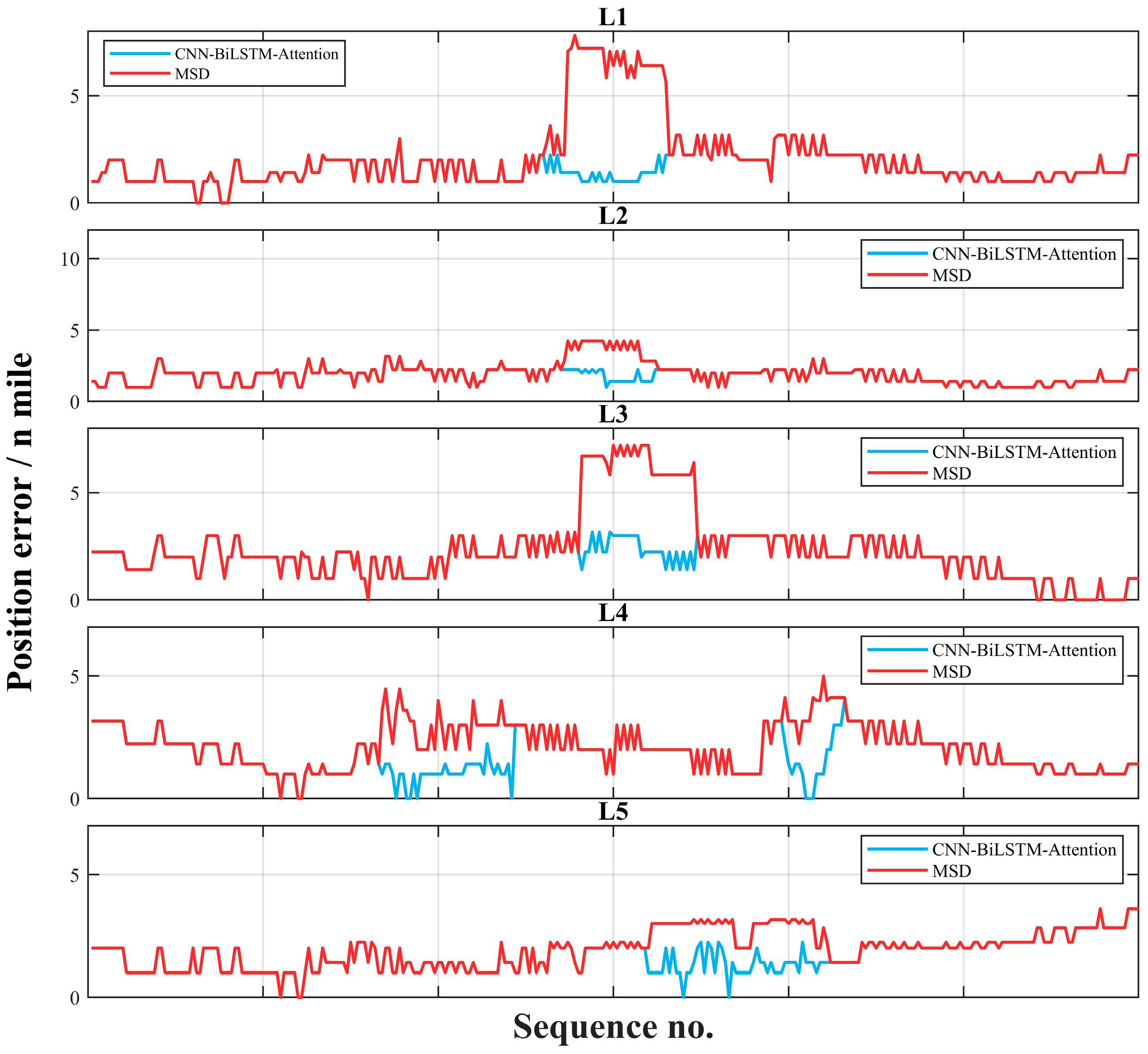
Trajectories L1–L5 were used to examine the prediction performance in gravity field regions with different anomaly characteristics. The five trajectories were distributed across separate 500 × 500-grid matching areas with increasing gravity anomaly variability from Area 01 to Area 05, corresponding to AGD values [17] of 0.93, 1.15, 1.50, 2.59, and 3.49 mGal per nautical mile, respectively. For each trajectory, an independent dataset was constructed from its corresponding MSD matching output, and a separate CNN–BiLSTM–Attention model was trained. Data from different trajectories were not mixed during training, while the network architecture and hyperparameter settings remained unchanged. The original MSD matching errors and corresponding prediction results for L1–L5 are presented in Figure 9. Quantitative results based on the five performance indicators defined above are summarized in

Table 3. Compensation performance of CNN–BiLSTM–Attention with MSD matching in different sea areas.

Track	APE-O (n Miles)	MSR-O (%)	APE-T (n Miles)	Recall-O (%)	IT (ms)
L1	1.34 ± 0.04	87.95 ± 2.60	1.56 ± 0.05	98.48 ± 1.36	17.25 ± 1.82
L2	1.78 ± 0.05	59.03 ± 2.21	1.76 ± 0.05	96.94 ± 2.04	15.49 ± 1.58
L3	2.37 ± 0.08	53.37 ± 2.20	1.91 ± 0.06	62.91 ± 2.15	17.17 ± 1.90
L4	1.19 ± 0.04	89.07 ± 2.19	1.75 ± 0.06	92.64 ± 2.16	14.18 ± 1.63
L5	1.31 ± 0.04	91.14 ± 2.18	1.66 ± 0.05	98.68 ± 1.32	16.37 ± 1.90

as the mean and standard deviation of five independent runs.

Figure 9 shows that the MSD matching errors differ considerably among the five gravity field regions in terms of amplitude, duration, and temporal distribution. The CNN–BiLSTM–Attention model reduces the principal error peaks in the identified outlier error intervals, although the quantitative performance remains region-dependent. As summarized in Table 3, L4 achieves the lowest APE-O of 1.19 ± 0.04 nautical miles, followed by L5 and L1 with 1.31 ± 0.04 and 1.34 ± 0.04 nautical miles, respectively. Their MSR-O values are also relatively high, reaching 89.07 ± 2.19%, 91.14 ± 2.18%, and 87.95 ± 2.60%. For L2, Recall-O remains high at 96.94 ± 2.04%, whereas MSR-O decreases to 59.03± 2.21%, indicating that most gross-error samples are identified but a smaller proportion of the predicted results satisfy the 2-nautical-mile criterion. L3 presents the most challenging case, with an APE-O of 2.37 ± 0.08 nautical miles, an MSR-O of 53.37 ± 2.20%, and a Recall-O of 62.91 ± 2.1%. This variation indicates that the prediction performance is influenced not only by the overall gravity anomaly variability represented by AGD, but also by the local structure and temporal distribution of the matching errors. Across L1–L5, APE-T remains between 1.566 and 1.918 nautical miles, while the inference time shows only limited variation. The relatively small standard deviations obtained from five independent runs indicate stable repeatability for each independently trained regional dataset.

3.2.3. Robustness Evaluation Under Variable Measurement Conditions

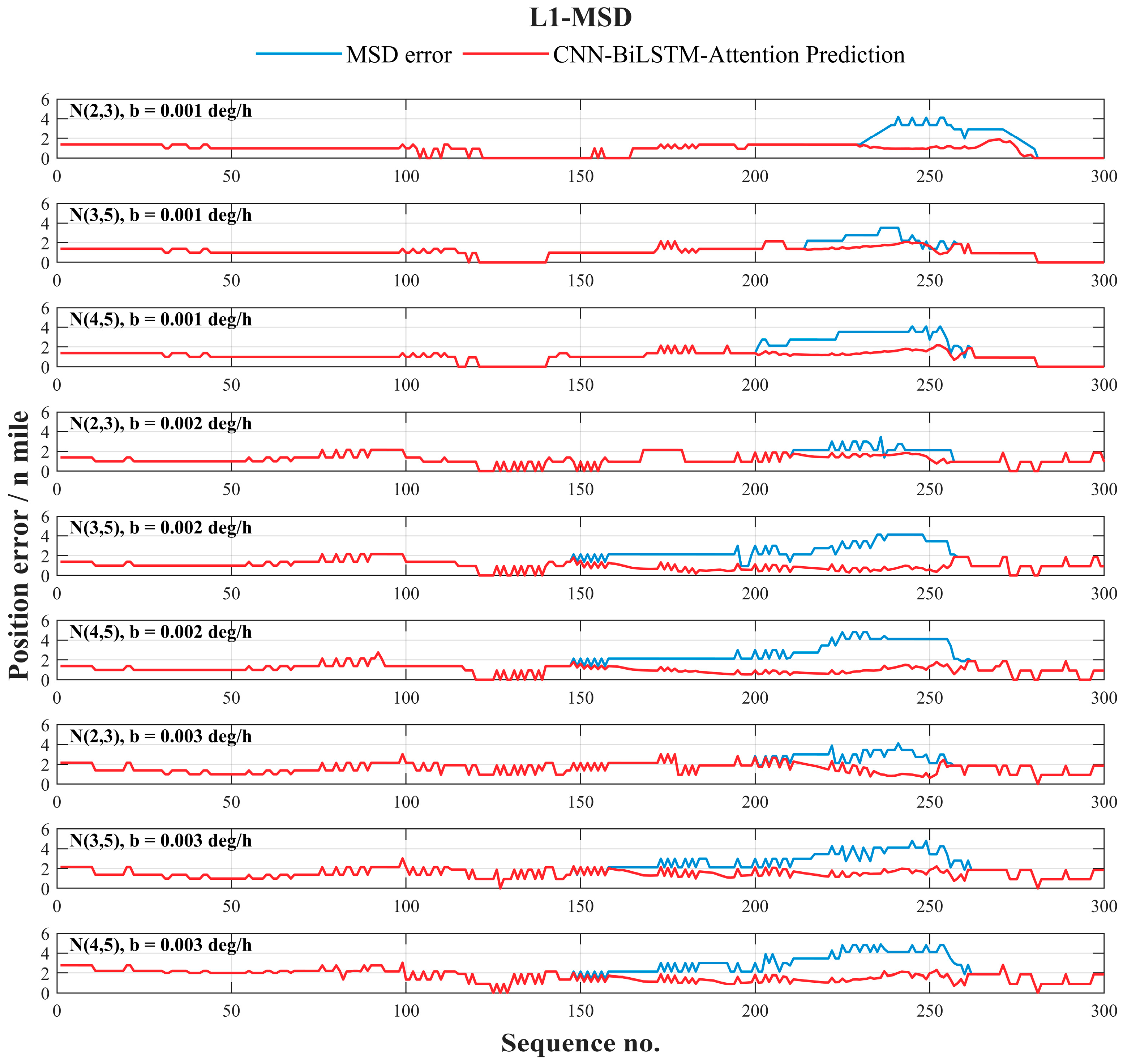
The L1 trajectory was processed using the MSD gravity matching method under nine measurement conditions. These conditions combined three Gaussian gravity noise distributions, $N(2,3)$, $N(3,5)$, and $N(4,5)$, with three INS gyroscope-bias levels of 0.001, 0.002, and 0.003°/h. The gravity matching and network parameters were set according to Section 3.1.

As shown in Figure 10, the CNN–BiLSTM–Attention model reduces the principal MSD error segments under all combinations of the three gravity noise distributions and three gyroscope-bias levels. The prediction is particularly stable at 0.001 and 0.002°/h, while larger residual fluctuations remain at 0.003°/h; nevertheless, clear error reduction is still observed. As summarized in

Table 4. Compensation performance of the proposed model for the L1 MSD matching results under different gravity measurement noise and INS gyroscope-bias conditions.

Gravity Noise	Gyroscope Bias (°/h)	APE-O (n Miles)	MSR-O (%)	APE-T (n Miles)	Recall-O (%)	IT (ms)
$N\left(2,3\right)$	0.001	1.08 ± 0.052	97.95 ± 1.92	0.89 ± 0.036	98.08 ± 1.82	18.85 ± 2.00
$N\left(3,5\right)$	0.001	1.55 ± 0.073	92.42 ± 3.60	1.07 ± 0.044	97.47 ± 1.40	15.05 ± 1.50
$N\left(4,5\right)$	0.001	1.41 ± 0.063	95.79 ± 2.92	1.04 ± 0.045	97.66 ± 1.41	16.05 ± 1.64
$N\left(2,3\right)$	0.002	1.50 ± 0.074	97.79 ± 1.48	1.17 ± 0.053	97.92 ± 1.47	12.59 ± 1.36
$N\left(3,5\right)$	0.002	0.75 ± 0.036	98.91 ± 0.73	0.99 ± 0.036	98.98 ± 0.73	13.81 ± 1.36
$N\left(4,5\right)$	0.002	0.97 ± 0.045	98.87 ± 0.72	1.04 ± 0.045	98.95 ± 0.73	13.82 ± 1.37
$N\left(2,3\right)$	0.003	1.55 ± 0.071	74.60 ± 4.88	1.58 ± 0.071	89.60 ± 3.91	13.91 ± 1.27
$N\left(3,5\right)$	0.003	1.56 ± 0.071	86.20 ± 4.66	1.50 ± 0.062	99.20 ± 1.79	13.77 ± 1.32
$N\left(4,5\right)$	0.003	1.42 ± 0.055	92.40 ± 3.21	1.69 ± 0.060	98.60 ± 1.95	13.76 ± 1.09

, APE-O remains between 0.75 and 1.56 n miles and below 2 n miles in all nine conditions, with MSR-O ranging from 74.60% to 98.91%. APE-T ranges from 0.89 to 1.69 nautical miles, and the prediction time is 12.59–18.85 ms per sample. These results indicate that the model maintains effective short-duration error prediction under the evaluated gravity noise and gyroscope-bias variations.

3.3. Dynamically Measured Gravity Experiment

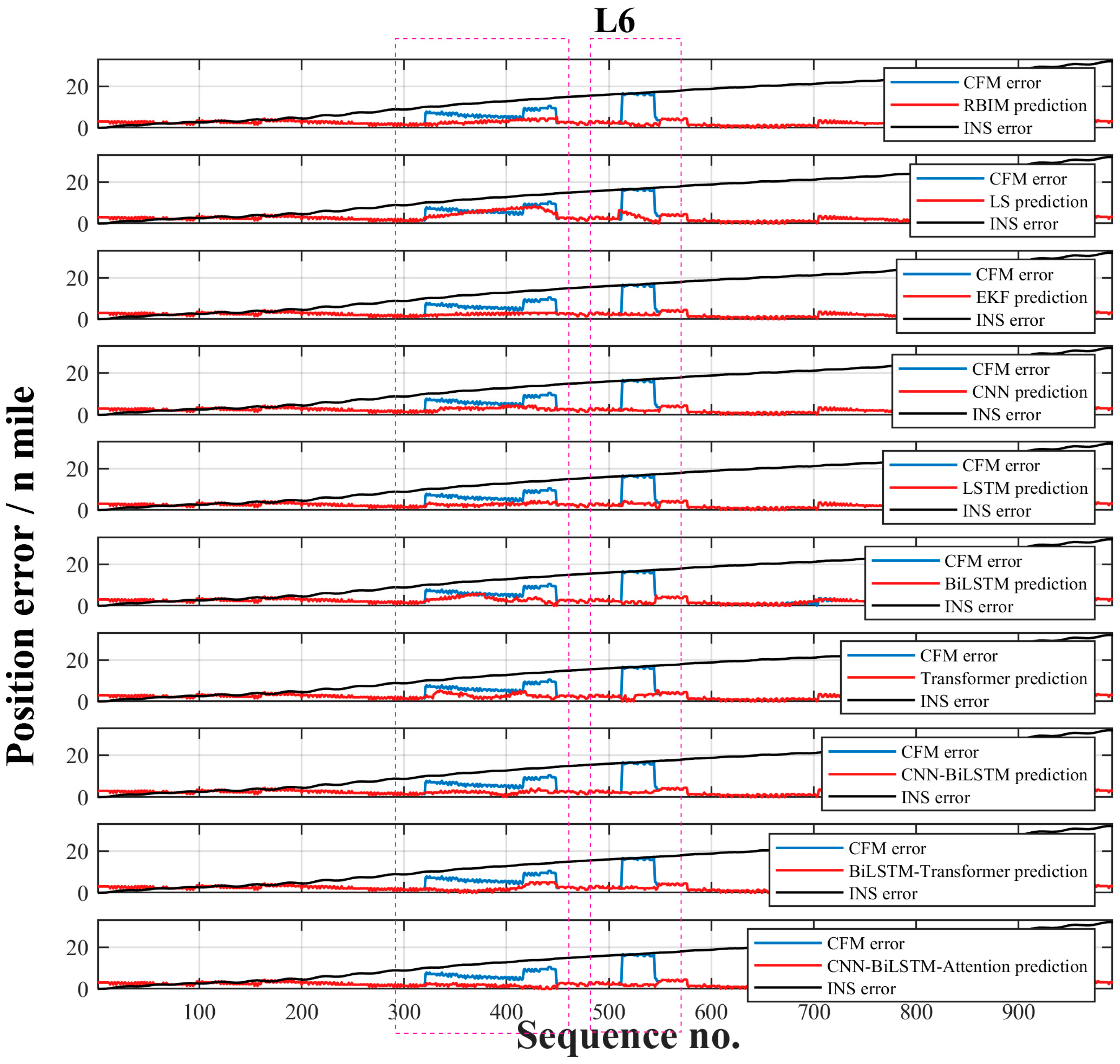
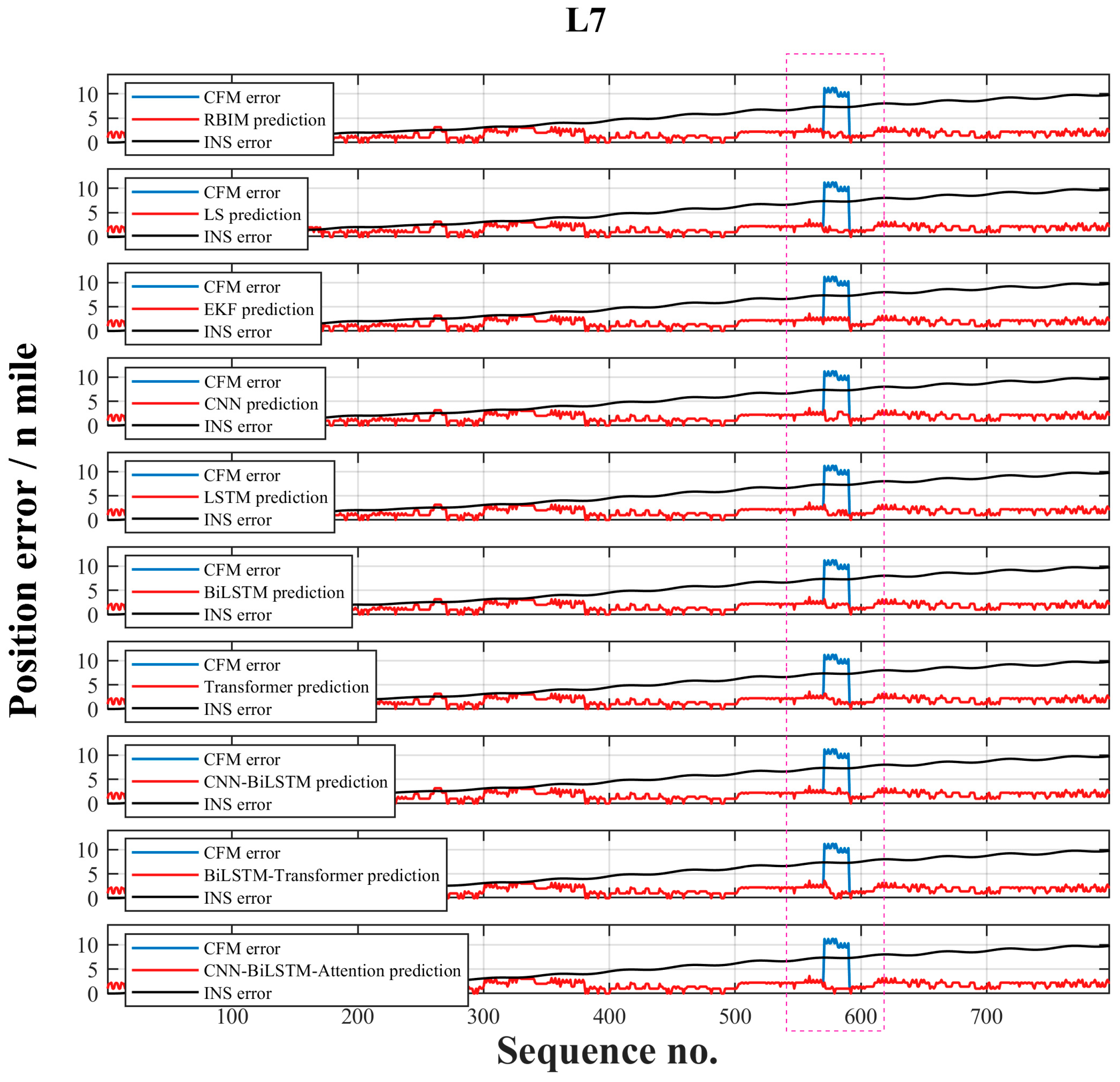
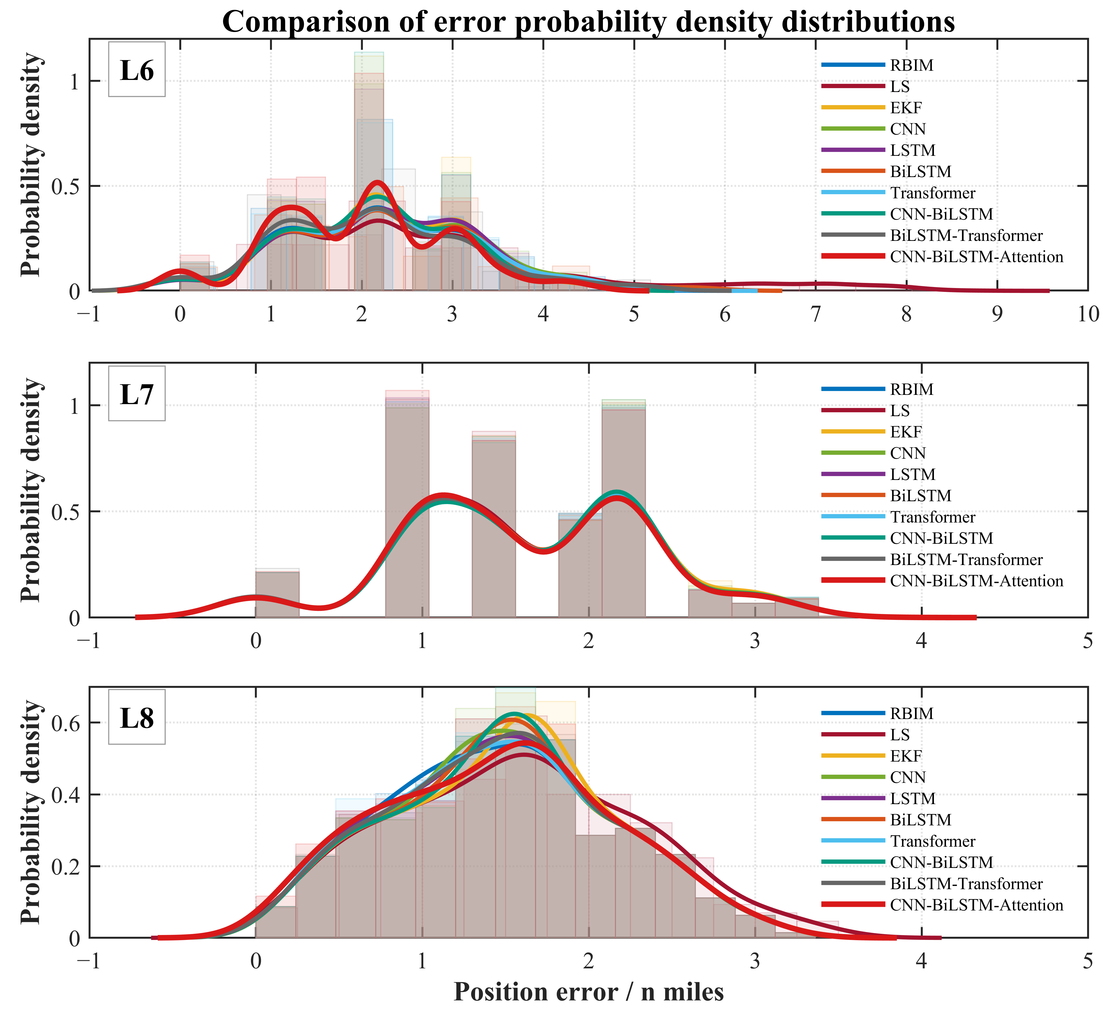
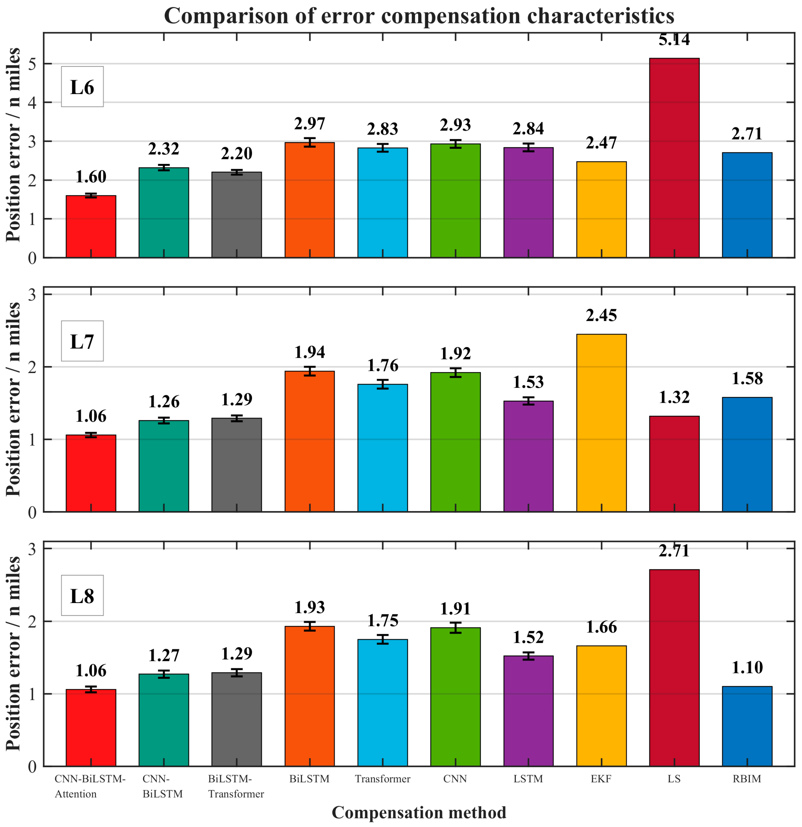
Experiments using three gravity datasets collected in the South China Sea were conducted to evaluate the matching error compensation performance of the proposed CNN–BiLSTM–Attention framework. For comparative assessment, several representative baseline approaches were considered, including RBIM, LS, EKF, CNN, LSTM, BiLSTM, Transformer, CNN–BiLSTM, and BiLSTM–Transformer. Five key performance indicators include the APE-O, MSR-O, Recall-O, APE-T, and IT, which are reported in

Table 5. Error compensation statistics for various algorithms applied to outliers in marine experiments.

Track	Method	APE-O (n Miles)	MSR-O (%)	APE-T (n Miles)	Recall-O (%)	IT (ms)
L6	RBIM	2.71	30.58	2.19	48.82	-
	LS	5.14	7.64	2.61	9.41	-
	EKF	2.47	34.71	2.15	58.82	-
	CNN	2.93 ± 0.10	20.68 ± 2.96	2.23 ± 0.07	36.25 ± 4.78	14.76 ± 1.80
	LSTM	2.84 ± 0.10	9.12 ± 3.27	2.20 ± 0.08	32.75 ± 4.31	10.95 ± 1.16
	BiLSTM	2.97 ± 0.11	28.34 ± 3.42	2.25 ± 0.08	40.38 ± 3.90	13.47 ± 1.50
	Transformer	2.83 ± 0.10	27.94 ± 4.05	2.22 ± 0.07	43.64 ± 4.17	21.48 ± 2.32
	CNN–BiLSTM	2.32 ± 0.07	31.91 ± 3.95	2.13 ± 0.06	71.59 ± 4.01	16.22 ± 1.74
	BiLSTM–Transformer	2.20 ± 0.06	54.16 ± 3.71	2.10 ± 0.05	73.77 ± 4.11	16.88 ± 1.91
	CNN–BiLSTM–Attention	1.60 ± 0.05	70.89 ± 3.35	2.00 ± 0.06	95.04 ± 2.92	21.32 ± 2.30
L7	RBIM	1.58	85.71	1.62	100.00	-
	LS	1.32	90.47	1.62	100.00	-
	EKF	2.45	4.76	1.65	57.14	-
	CNN	1.92 ± 0.06	47.56 ± 7.03	1.64 ± 0.05	76.04 ± 7.42	16.04 ± 1.90
	LSTM	1.53 ± 0.05	89.89 ± 7.32	1.62 ± 0.05	95.28 ± 3.70	12.50 ± 1.43
	BiLSTM	1.94 ± 0.06	57.15 ± 7.23	1.65 ± 0.03	91.75 ± 4.22	15.52 ± 1.71
	Transformer	1.76 ± 0.06	66.81 ± 6.91	1.63 ± 0.05	90.73 ± 6.05	22.77 ± 2.17
	CNN–BiLSTM	1.26 ± 0.04	52.90 ± 6.91	1.60 ± 0.05	86.37 ± 6.90	18.85 ± 0.31
	BiLSTM- Transformer	1.29 ± 0.04	76.65 ± 6.78	1.60 ± 0.05	91.70 ± 6.55	18.02 ± 1.63
	CNN–BiLSTM–Attention	1.06 ± 0.03	94.50 ± 3.01	1.60 ± 0.05	97.78 ± 2.12	20.58 ± 1.92
L8	RBIM	1.10	100.00	1.46	100.00	-
	LS	2.71	0.00	1.56	43.14	-
	EKF	1.66	100.00	1.49	100.00	-
	CNN	1.91 ± 0.07	45.73 ± 6.33	1.47 ± 0.05	73.84 ± 6.56	15.72 ± 1.58
	LSTM	1.52 ± 0.05	87.89 ± 6.51	1.48 ± 0.05	94.14 ± 3.77	12.37 ± 1.32
	BiLSTM	1.93 ± 0.06	55.35 ± 6.60	1.47 ± 0.05	92.08 ± 5.45	16.34 ± 1.54
	Transformer	1.75 ± 0.06	65.31 ± 6.65	1.47± 0.05	88.94 ± 6.11	22.21 ± 2.29
	CNN–BiLSTM	1.27 ± 0.05	51.17 ± 7.07	1.46 ± 0.05	84.87 ± 6.75	16.48 ± 1.67
	BiLSTM- Transformer	1.29 ± 0.05	74.21 ± 6.70	1.47 ± 0.05	89.77 ± 7.18	17.22 ± 1.70
	CNN–BiLSTM–Attention	1.06 ± 0.04	94.20 ± 3.35	1.45 ± 0.05	98.31 ± 2.33	20.54 ± 2.02

. For the original CFM results, the complete-trajectory APE-T values of L6, L7, and L8 were 3.16, 1.85, and 1.67 n miles, respectively, while the corresponding overall matching success rates under the 2-n-mile criterion were 38.81%, 64.54%, and 71.16%. In addition, the compensation performance in regions containing outliers is illustrated in Figure 11, Figure 12 and Figure 13, while the statistical characteristics of positioning errors derived from the marine experiments are presented in Figure 14 and Figure 15 through multiple subplots. The hyperparameters, parameter counts, and tuning ranges used for all compared models are summarized in Appendix A (

Table A1. Configurations of representative error compensation methods.

Model	Main Network Configuration	Hidden/Feature Dimension	Attention Heads	Dropout	Initial Learning Rate	Epochs	Mini Batch	Parameters (m)
CNN	4Conv blocks + 3 FC layers	Conv: 32, 64, 128, 256; FC: 128, 64, 2	N/A	0.3, 0.2	8 × 10−3	100	32	2.2
LSTM	3LSTM layers + 2 FC layers	LSTM: 128, 256, 128; FC: 64, 2	N/A	0.2, 0.2, 0.3, 0.2	8 × 10−3	200	32	0.7
BiLSTM	3BiLSTM layers + 3FC layers	BiLSTM: 128, 256, 128; FC: 64, 32, 2	N/A	0.2, 0.2, 0.3, 0.2	3 × 10−3	200	32	2
Transformer	3Transformer encoder blocks + FC head	Model dimension = 128; FFN = 512; FC: 256, 128, 2	8	0.2; FC dropout 0.3	5 × 10−3	200	32	0.8
CNN–BiLSTM	3Conv layers + 2 BiLSTM layers + FC regression	Conv: 32, 64, 128; BiLSTM: 256, 512; FC: 128, 2	N/A	0.2, 0.3	8 × 10−3	200	32	1.5
BiLSTM–Transformer	3 BiLSTM layers + self-attention + FFN + FC	BiLSTM: 128, 128, 64; FFN: 512→128; FC: 64→2	4	0.2, 0.2, 0.1, 0.1, 0.3, 0.2	2 × 10−3	200	32	4
CNN–BiLSTM–Attention	3Conv layers + 2 BiLSTM layers + Attention module + FC regression	Conv: 32, 64, 128; BiLSTM: 256, 512; FC: 256, 128, 2	1	0.2, 0.3, 0.3	8 × 10−3	200	32	4.2

).

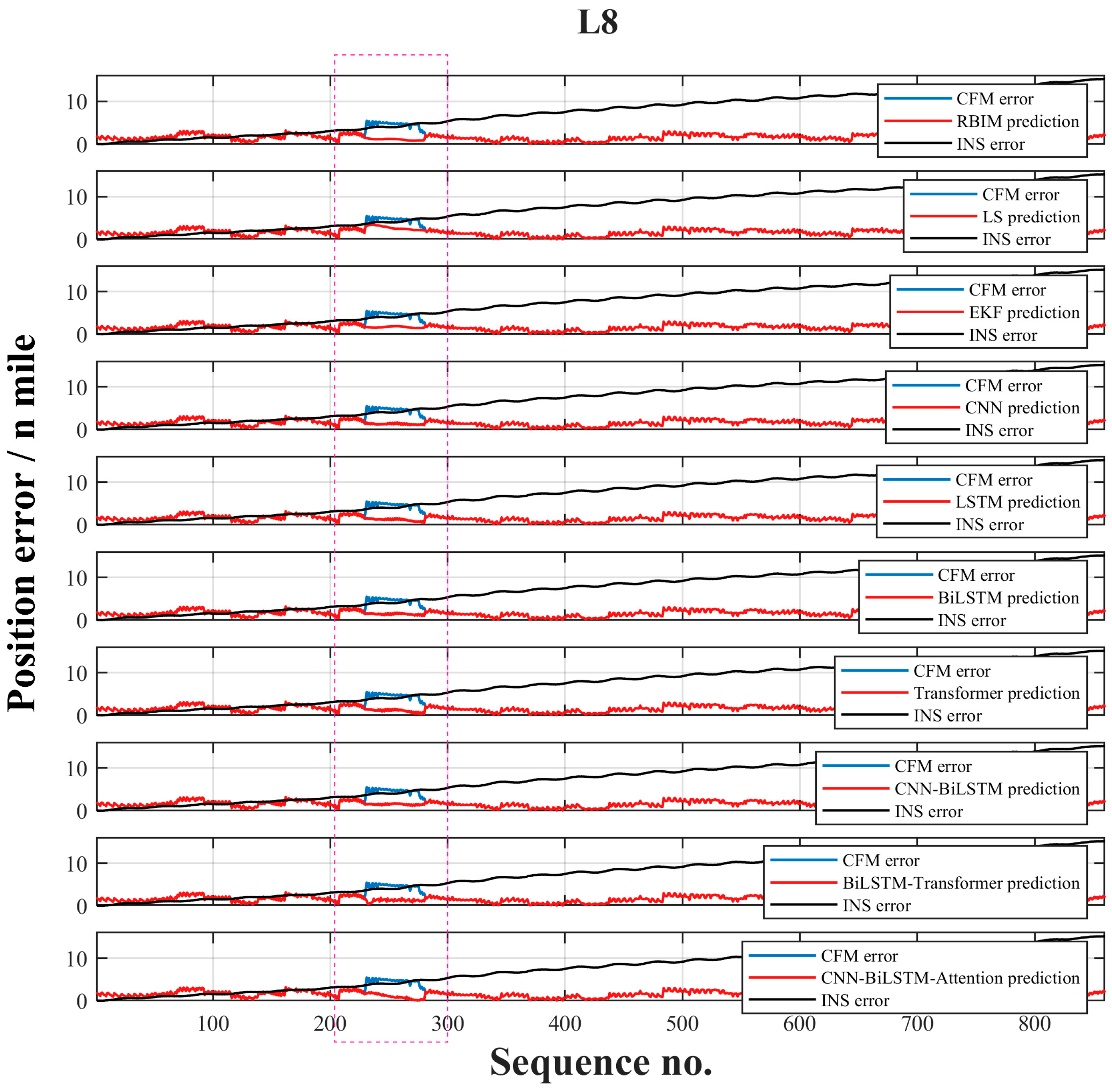
The error curves for L6–L8 show that the measured trajectories contain gross matching errors with different durations and amplitudes. L6 contains two relatively long error intervals, whereas L7 is characterized by a short and abrupt error segment, and L8 exhibits a moderate error increase over a continuous interval. The compensation results indicate that the CNN–BiLSTM–Attention model reduces the principal error peaks in all three trajectories. The improvement is particularly evident on L6, where several conventional and learning-based methods retain relatively large residual errors within the two gross-error intervals. Based on five independent runs, the proposed method yielded 95% confidence intervals of [1.53, 1.67], [1.01, 1.10], and [1.01, 1.11] nautical miles for APE-O on L6–L8, respectively, while two-sided Welch’s tests against BiLSTM–Transformer indicated statistically significant reductions on all three trajectories (p < 0.001). The unaided INS position errors are also included in Figure 11, Figure 12 and Figure 13 as a reference baseline. The INS errors gradually increase along the measured trajectories because of continuous inertial integration, whereas the gravity matching solutions generally remain more accurate outside the identified error intervals owing to map-referenced updates. For RBIM, the last available gravity matching position is propagated using subsequent INS-derived position increments over the identified error interval, providing an INS-increment-based propagation baseline. As the interval becomes longer, the reconstructed solution may progressively inherit accumulated inertial drift.

As summarized in Table 5, the proposed method achieves an APE-O of 1.60 ± 0.05 nautical miles on L6, compared with 2.20 ± 0.06 nautical miles for BiLSTM–Transformer. Compared with the INS-increment-based RBIM baseline, the APE-O is reduced from 2.71 to 1.60 nautical miles on L6, from 1.58 to 1.06 nautical miles on L7, and from 1.10 to 1.06 nautical miles on L8. On L6, its MSR-O and Recall-O reach 70.89 ± 3.35% and 95.04 ± 2.92%, respectively, indicating improved compensation for the more complex error intervals. The larger performance difference from RBIM on L6 is consistent with its two relatively long error intervals, over which an INS-increment-based propagation solution is more susceptible to accumulated inertial drift. On L7, the proposed method obtains the lowest APE-O of 1.06 ± 0.03 nautical miles and the highest MSR-O among the learning-based methods, reaching 94.50 ± 3.01%. Its APE-T remains comparable to those of the other methods because the gross-error interval occupies only a small portion of the complete trajectory. On L8, the proposed method achieves an APE-O of 1.06 ± 0.04 nautical miles, which is lower than those of the other learning-based models. RBIM and EKF both achieve MSR-O and Recall-O values of 100% on this trajectory, demonstrating the effectiveness of conventional methods for relatively regular and localized error patterns, whereas the proposed model shows a clearer advantage for complex or extended matching error intervals, such as those observed on L6. This behavior is consistent with the motivation for jointly using INS motion information and gravity anomaly measurements rather than relying solely on INS-increment propagation during degraded matching intervals. Across L6–L8, the proposed CNN–BiLSTM–Attention model consistently reduced the complete-trajectory APE-T by 13.2–36.7% relative to the original CFM results, indicating that the compensation improved the overall quality of the gravity matching position updates.

The probability density distributions further show that the proposed method shifts the corrected-error distribution toward lower values, particularly on L6. The distributions on L7 and L8 exhibit greater overlap because the differences among the corrected results are comparatively smaller. The inference time of the proposed model ranges from 20.54 to 21.32 ms, which is comparable to that of the Transformer-based methods, although it is not the lowest among the evaluated models. In addition, the relatively small standard deviations obtained over five independent runs indicate stable repeatability of the learning-based results on the three measured trajectories.

4. Discussion

Across the simulation and marine experiments, the proposed CNN–BiLSTM–Attention framework reduced the principal errors within the identified matching error intervals under different gravity field characteristics, matching algorithms, and measurement conditions. In the simulation experiments, the five gravity field regions covered AGD values from 0.93 to 3.49 mGal per nautical mile, and error reduction was observed for all five gravity matching algorithms. The results varied across regions and matching outputs, indicating that compensation performance depends not only on overall gravity field variability but also on the local structure and temporal distribution of matching errors. In the marine experiments, the proposed method showed strong error compensation performance on L6 and L7, where the error intervals were relatively complex or extended. On L8, conventional methods also remained effective for the more regular and localized error pattern, indicating that the relative advantage of different approaches depends on the characteristics of the matching degradation. The comparison between CNN–BiLSTM and CNN–BiLSTM–Attention further indicates that the attention-based architecture can improve prediction performance in the evaluated cases, although the independent contributions of all network components have not been fully separated. The inference time of approximately 21 ms supports the possibility of online use under the present experimental configuration, while onboard performance on embedded marine equipment still requires further verification.

The present results should be interpreted within the evaluated datasets and experimental settings. Reliable training samples were selected offline using reference positions and the 2-nautical-mile criterion, whereas online screening relies on the temporal consistency of gravity matching position increments. The revised trailing Hampel window uses only the current and preceding available increments and therefore does not require future samples. The fixed threshold provides effective screening for the evaluated data, although sustained or clustered noise may reduce detection sensitivity. In addition, the models were trained and tested separately for each trajectory; therefore, the reported results reflect temporal prediction on unseen segments of the same trajectory rather than cross-trajectory or cross-region generalization.

For consecutive flagged samples, the CNN–BiLSTM–Attention model is non-autoregressive because preceding prediction outputs are not used as network inputs. Nevertheless, residual increment errors may accumulate in the reconstructed position during extended compensation, particularly over long consecutive matching error intervals. This issue is more relevant to the relatively long error intervals of L6. Once reliable gravity matching updates resume, such accumulation is interrupted. Therefore, prolonged continuous matching failures remain a limitation of the current framework and may require additional aiding, dedicated outage estimation, or gravity matching reinitialization.

Future work will investigate adaptive Hampel-window and threshold selection under varying measurement conditions, together with uncertainty-aware prediction and strategies for sustained matching outages. More complete component-wise ablation experiments, long-duration tests with consecutive matching error intervals, and implementation on embedded navigation hardware will be conducted to clarify the contribution of individual modules, investigate error propagation during sustained matching degradation, and assess practical onboard performance. In addition, unified training using data from multiple gravity field regions will be evaluated through leave-one-trajectory-out or leave-one-region-out validation to further examine cross-region applicability.

5. Conclusions

This study developed a CNN–BiLSTM–Attention-based matching error compensation framework for gravity aided inertial navigation. The framework operates between gravity matching and INS fusion, using the temporal sequences of INS position increments and gravity anomaly measurements to predict compensation increments for potentially unreliable gravity matching outputs. For the marine experiments, synchronized GNSS positions were used only as offline reference data for training-sample selection and performance evaluation; they were not used as inputs during online compensation. Its performance was evaluated using five simulated trajectories covering AGD values from 0.93 to 3.49 mGal per nautical mile and three marine trajectories collected under different measurement conditions. Across the evaluated trajectories and gravity matching methods, the compensated results showed reductions in the average position error in outlier segments (APE-O), together with increases in the matching success rate (MSR-O) and outlier recall rate (Recall-O). In the marine experiments, the mean APE-O values were 1.60, 1.06, and 1.06 nautical miles for L6, L7, and L8, respectively, while the corresponding mean MSR-O values were 70.89%, 94.50%, and 94.20%. Recall-O remained above 95% for all three trajectories. The error distributions also exhibited reduced large-error dispersion after compensation. The inference time was short relative to the gravity matching update interval under the present experimental configuration. These results characterize the compensation performance of the proposed framework within the evaluated gravity field regions, trajectories, and matching configurations. Further work will investigate cross-region transfer, adaptive confidence analysis, and onboard deployment on embedded navigation hardware.

References

1. Rice, H.; Mendelsohn, L.; Aarons, R.; Mazzola, D. Next generation marine precision navigation system. In Proceedings of the IEEE 2000 Position Location and Navigation Symposium (PLANS), San Diego, CA, USA, 13–16 March 2000; pp. 200–206. [Google Scholar] [CrossRef] [Scilit]
2. Yang, Y.; Xu, T.; Xue, S. Progresses and prospects in developing marine geodetic datum and marine navigation of China. J. Geod. Geoinf. Sci. 2017, 46, 1–8. [Google Scholar] [CrossRef]
3. Jekeli, C. Precision free-inertial navigation with gravity compensation by an onboard gradiometer. J. Guid. Control Dyn. 2006, 29, 704–713. [Google Scholar] [CrossRef] [Scilit]
4. Xue, S.; Yang, Y.; Yang, W. Single-differenced models for GNSS-acoustic seafloor point positioning. J. Geod. 2022, 96, 38. [Google Scholar] [CrossRef] [Scilit]
5. Wu, L.; Wang, H.; Chai, H.; Zhang, L.; Hsu, H.; Wang, Y. Performance evaluation and analysis for gravity matching aided navigation. Sensors 2017, 17, 769. [Google Scholar] [CrossRef] [Scilit] [PubMed]
6. Chen, H.; Taha, T.M.; Chodavarapu, V.P. Towards improved inertial navigation by reducing errors using deep learning methodology. Appl. Sci. 2022, 12, 3645. [Google Scholar] [CrossRef] [Scilit]
7. Chang, L.; Qin, F.; Wu, M. Gravity disturbance compensation for inertial navigation system. IEEE Trans. Instrum. Meas. 2019, 68, 3751–3765. [Google Scholar] [CrossRef] [Scilit]
8. Han, Y.; Wang, B.; Deng, Z.; Fu, M. A matching algorithm based on the nonlinear filter and similarity transformation for gravity-aided underwater navigation. IEEE/ASME Trans. Mechatron. 2018, 23, 646–654. [Google Scholar] [CrossRef]
9. Golden, J.P. Terrain contour matching (TERCOM): A cruise missile guidance aid. In Proceedings of the SPIE 238, Image Processing for Missile Guidance, San Diego, CA, USA, 23 December 1980; pp. 10–18. [Google Scholar] [CrossRef] [Scilit]
10. Wang, K.; Lei, Y.; Deng, W.; Zhang, J. Research on iterative closest contour point for underwater terrain-aided navigation. In Proceedings of the Joint IAPR International Workshops, SSPR 2006 and SPR 2006, Hong Kong, China, 17–19 August 2006; pp. 252–260. [Google Scholar] [CrossRef] [Scilit]
11. Wang, Z.; Bian, S. A local geopotential model for implementation of underwater passive navigation. Prog. Nat. Sci. 2008, 18, 1139–1145. [Google Scholar] [CrossRef] [Scilit]
12. Wu, X.; Li, S. Progress of underwater gravity-aided inertial navigation. In China National Report on Geodesy; Technical Report; Chinese National Committee for The International Union of Geodesy and Geophysics: Beijing, China, 2011. [Google Scholar]
13. Han, Y.; Wang, B.; Deng, Z.; Fu, M. Point mass filter based matching algorithm in gravity aided underwater navigation. J. Syst. Eng. Electron. 2018, 29, 152–159. [Google Scholar] [CrossRef] [Scilit]
14. Zong, J.; Bian, S.; Tong, Y.; Ji, B.; Li, H.; Xi, M. Classification of gravity matching areas using PSO-BP neural networks based on PCA and satellite altimetry data over the western Pacific. Sensors 2022, 22, 9892. [Google Scholar] [CrossRef] [Scilit] [PubMed]
15. Wang, Y.; Deng, Z.; Zhang, P.; Wang, B.; Zhao, S. A gravity-aided navigation matching algorithm based on triangulation. IEEE Sens. J. 2024, 24, 34851–34861. [Google Scholar] [CrossRef] [Scilit]
16. Liu, S.; Wu, L.; Li, Q.; Bao, L.; Wang, Y. Gravity matching navigation algorithm based on spatial-frequency multidimensional feature fusion. IEEE Trans. Instrum. Meas. 2025, 74, 8511212. [Google Scholar] [CrossRef] [Scilit]
17. Liu, H.; Wu, L.; Bao, L.; Li, Q.; Zhang, P.; Wang, Y. Gravity matching navigation algorithm based on multiscale search and Hadamard transformed difference. ISA Trans. 2022, 128, 409–422. [Google Scholar] [CrossRef] [Scilit] [PubMed]
18. Liu, H.; Wu, L.; Bao, L.; Li, Q.; Zhang, P.; Xi, M.; Wang, Y. Comprehensive features matching algorithm for gravity aided navigation. IEEE Geosci. Remote Sens. Lett. 2022, 19, 1505305. [Google Scholar] [CrossRef] [Scilit]
19. Zhao, S.; Dou, Z.; Zhu, H.; Zheng, W.; Shen, Y. Gravity-aided navigation of underwater vehicles via alternating line small-domain matching method. IEEE Trans. Instrum. Meas. 2025, 74, 3002609. [Google Scholar] [CrossRef] [Scilit]
20. Luo, K.; Cai, S.; Yu, R.; Cao, J.; Guo, Y. Robust two-stage filtering for INS/gravity matching passive integrated navigation systems. IEEE Sens. J. 2022, 22, 3370–3381. [Google Scholar] [CrossRef] [Scilit]
21. Wang, Z.; Huang, Y.; Wang, M.; Wu, J.; Zhang, Y. A computationally efficient outlier-robust cubature Kalman filter for underwater gravity matching navigation. IEEE Trans. Instrum. Meas. 2022, 71, 8500418. [Google Scholar] [CrossRef] [Scilit]
22. Wang, B.; Zhu, J.; Ma, Z.; Deng, Z.; Fu, M. Improved particle filter-based matching method with gravity sample vector for underwater gravity-aided navigation. IEEE Trans. Ind. Electron. 2021, 68, 5206–5216. [Google Scholar] [CrossRef] [Scilit]
23. Mao, N.; Li, A.; Xu, J.; Li, F.; Qin, F.; He, H.; Li, J.; Zhu, B. Adaptive gravity-aided inertial navigation based on characteristic analysis of marine gravity anomaly from satellite altimetry. IEEE Trans. Geosci. Remote Sens. 2024, 62, 5920813. [Google Scholar] [CrossRef] [Scilit]
24. Goncharov, V.K.; Klementieva, N.Y. Parameterization of the propeller thrust for modelling ship braking in ice channel behind icebreaker. Transp. Saf. Environ. 2023, 5, tdac042. [Google Scholar] [CrossRef] [Scilit]
25. Chen, X.; Zhang, Y.; Feng, Z.; Zhang, H.; Biancardo, S.A.; Shang, W.-L. Spatiotemporal ship carbon emission exploitation and low-carbon shipping pathway evaluation. Appl. Energy 2026, 422, 128334. [Google Scholar] [CrossRef] [Scilit]
26. Chen, X.; Wu, P.; Wang, Z.; Feng, Z.; Luo, L.; Zhang, H.; Biancardo, S.A. MKG-GNN: Maritime knowledge graph and GNN framework for ship speed forecasting in port. Ocean Eng. 2026, 355, 125179. [Google Scholar] [CrossRef] [Scilit]
27. Gidugu, A.R.; Vandavasi, B.N.J.; Narayanaswamy, V. Bio-inspired machine-learning aided geo-magnetic field based AUV navigation system. Sci. Rep. 2024, 14, 17912. [Google Scholar] [CrossRef] [Scilit]
28. Heshmat, M.; Saad Saoud, L.; Abujabal, M.; Sultan, A.; Elmezain, M.; Seneviratne, L.; Hussain, I. Underwater SLAM meets deep learning: Challenges, multi-sensor integration, and future directions. Sensors 2025, 25, 3258. [Google Scholar] [CrossRef] [Scilit] [PubMed]
29. Palomeras, N.; Ridao, P. Autonomous underwater vehicle docking under realistic assumptions using deep reinforcement learning. Drones 2024, 8, 673. [Google Scholar] [CrossRef] [Scilit]
30. Topini, E.; Fanelli, F.; Topini, A.; Pebody, M.; Ridolfi, A.; Phillips, A.B.; Allotta, B. An experimental comparison of deep learning strategies for AUV navigation in DVL-denied environments. Ocean Eng. 2023, 274, 114034. [Google Scholar] [CrossRef] [Scilit]
31. Hewitson, S.; Wang, J. GNSS receiver autonomous integrity monitoring (RAIM) performance analysis. GPS Solut. 2006, 10, 155–170. [Google Scholar] [CrossRef] [Scilit]
32. Joshi, B.; Damron, H.; Rahman, S.; Rekleitis, I. SM/VIO: Robust underwater state estimation switching between model-based and visual inertial odometry. In Proceedings of the 2023 IEEE International Conference on Robotics and Automation (ICRA), London, UK, 29 May–2 June 2023; pp. 5192–5199. [Google Scholar] [CrossRef] [Scilit]
33. Hassan, S.; Byun, H.; Kim, J. Iterative smoothing and outlier detection for underwater navigation. In Proceedings of the Australasian Conference on Robotics and Automation (ACRA), Sydney, Australia, 1–3 December 2021. [Google Scholar] [CrossRef] [Scilit]
34. Chen, R.; Zhao, L. Multi-level autonomous integrity monitoring method for multi-source PNT resilient fusion navigation. Satell. Navig. 2023, 4, 21. [Google Scholar] [CrossRef] [Scilit]
35. Tal, A.; Klein, I.; Katz, R. Inertial navigation system/Doppler velocity log (INS/DVL) fusion with partial DVL measurements. Sensors 2017, 17, 415. [Google Scholar] [CrossRef] [Scilit] [PubMed]
36. Du, N.; Yu, H.; Sheng, H.; He, Q.; Tu, J.; Han, Z. An approach based on BiLSTM-Transformer for marine inertial navigation. In Proceedings of the 4th International Symposium on Computer Applications and Information Technology (ISCAIT), Xi’an, China, 21–23 March 2025; pp. 1039–1042. [Google Scholar] [CrossRef] [Scilit]
37. Jiang, Y.; Zhou, Z.; Zhang, Y.; Yang, H.; Gao, Y. Deep-learning-enhanced outlier detection for precise GNSS positioning with smartphones. IEEE Trans. Instrum. Meas. 2025, 74, 2526013. [Google Scholar] [CrossRef] [Scilit]
38. Yan, J.; Li, X.; Yang, M.; Gao, M.; Fang, Z.; Sun, R.; Xu, Y. A novel adaptive random error model integrity monitoring algorithm for low Earth orbit enhanced navigation. IEEE Trans. Instrum. Meas. 2025, 74, 8514316. [Google Scholar] [CrossRef] [Scilit]
39. Shao, J.; Chen, W.; Wang, J.; Yu, F.; Weng, D.; Zhang, Y. Sequential integrity monitoring with state-domain consistency detection for integrated navigation in adverse urban areas. IEEE Trans. Instrum. Meas. 2025, 74, 8509611. [Google Scholar] [CrossRef] [Scilit]
40. Liu, P.; Wang, B.; Li, Z.; Zhu, Z.; Liang, J. A positioning error correction method for dead-reckoning navigation of underwater vehicles. IEEE Trans. Instrum. Meas. 2025, 74, 8512513. [Google Scholar] [CrossRef] [Scilit]
41. Ali, T.H.; Taha, H.H.; Sedeeq, B.S.; Hayawi, H.A.A. Novel Hampel filtering and robust regression in control chart applications for regression process monitoring. J. Stat. Theory Appl. 2025, 24, 842–860. [Google Scholar] [CrossRef] [Scilit]
42. Wang, J.; Jiang, W.; Li, Z.; Lu, Y. A new multi-scale sliding window LSTM framework (MSSW-LSTM): A case study for GNSS time-series prediction. Remote Sens. 2021, 13, 3328. [Google Scholar] [CrossRef] [Scilit]
43. Bhatt, D.; Patel, C.; Talsania, H.; Patel, J.; Vaghela, R.; Pandya, S.; Modi, K.; Ghayvat, H. CNN variants for computer vision: History, architecture, application, challenges and future scope. Electronics 2021, 10, 2470. [Google Scholar] [CrossRef] [Scilit]
44. Sandwell, D.T.; Müller, R.D.; Smith, W.H.F.; Garcia, E.; Francis, R. New global marine gravity model from CryoSat-2 and Jason-1 reveals buried tectonic structure. Science 2014, 346, 65–67. [Google Scholar] [CrossRef] [Scilit] [PubMed]
45. Wu, P.; Wu, L.; Bao, L.; Wang, L.; Wang, B.; Tang, D. A marine gravimeter based on electromagnetic damping and its tests in the South China Sea. J. Oceanol. Limnol. 2023, 41, 792–803. [Google Scholar] [CrossRef] [Scilit]
Figure 1. Gravity matching–aided navigation system.
Jmse 14 01608 g001
Figure 2. CNN–BiLSTM–Attention model structure with gravity pattern construction for error compensation.
Jmse 14 01608 g002
Figure 3. Process of CNN–BiLSTM–Attention for error compensation. (a) Training process; (b) correction process.
Jmse 14 01608 g003
Figure 4. Gravity reference map with simulation and measured trajectories.
Jmse 14 01608 g004
Figure 5. Gravity anomaly contour maps of trajectories in simulation and marine experiments.
Jmse 14 01608 g005
Figure 6. Gravity measurement data and reference map data used in simulation.
Jmse 14 01608 g006
Figure 7. Marine gravity measurement data and reference map data.
Jmse 14 01608 g007
Figure 8. Error compensation performance for position estimates produced by the various matching algorithms in L1 simulation experiments.
Jmse 14 01608 g008
Figure 9. MSD matching errors and prediction results in different gravity field regions.
Jmse 14 01608 g009
Figure 10. Gravity matching errors and prediction results in different measurement conditions.
Jmse 14 01608 g010
Figure 11. Matching error compensation performance of different models on the L6. (The pink boxes indicate the gross-error intervals).
Jmse 14 01608 g011
Figure 12. Matching error compensation performance of different models on the L7. (The pink boxes indicate the gross-error intervals).
Jmse 14 01608 g012
Figure 13. Matching error compensation performance of different models on the L8. (The pink boxes indicate the gross-error intervals).
Jmse 14 01608 g013
Figure 14. Probability density distributions of position error across different algorithms for marine experiments.
Jmse 14 01608 g014
Figure 15. Compensation error bar chart across different algorithms for marine experiments.
Jmse 14 01608 g015