Multi-Scale CFD Investigation of Viscous Scale Effects on Bulbous Bow Slamming Pressures and Full-Scale Extrapolation

Abstract

Predicting wave slamming pressures on bulbous bows is essential for ship structural safety. This study employs an overset-grid RANS-VOF framework to investigate viscous scale effects on bulbous bow slamming loads. Multi-scale simulations were conducted across four geometric scale ratios of 1:50, 1:20, 1:15, and 1:10 (α = 50, 20, 15, 10) under critical pitch-heave resonant head waves (λ/L_WL = 1.2). While global motion responses follow Froude similitude, local dynamic slamming pressures show notable scale disparities. Smaller physical models develop a relatively thicker viscous boundary layer that acts as a hydrodynamic cushion, reducing peak pressures while broadening pulse durations. Consequently, direct Froude scaling from small-scale models tends to underestimate full-scale impact loads. To account for these viscous scale effects, an engineering extrapolation approach based on multi-scale regression is proposed, which demonstrates a reasonable linear correlation across the investigated range (R² = 0.88–0.99) in the primary impact region. This study provides physical insights into the scaling behavior of bulbous bow slamming and offers a practical reference for full-scale load estimation.

1. Introduction

Ship slamming, a sudden and highly nonlinear hydrodynamic impact between hull and water surface, poses extreme risks to marine structures [1,2,3]. Violent bow impacts generate severe local pressure peaks that vanish within milliseconds, yet these events can trigger localized structural damage and excite global hull girder vibrations (whipping) [4,5,6]. With its intricate 3D curved geometry at the forward tip, the bulbous bow suffers the most during large seakeeping motions [7,8]. Finding exact values for these concentrated loads remains critical for safe ship design.

In the past, most of the studies by researchers have used empirical formulas and simplified analytical tools, such as strip theories and Wagner-based models, for quick initial evaluations [9,10,11]. However, the above traditional techniques and linear potential flow solvers [12,13,14,15,16] are not suitable for modelling severe free-surface breaking, splash jets, and complex 3D flow separation around modern bulbous bows. Recently, Reynolds-averaged Navier–Stokes (RANS) solvers combined with the Volume of Fluid (VOF) method have become the standard options for predicting these extreme wave-body interactions [1,17,18,19,20,21,22,23]. Furthermore, recent investigations on stiffened panels [24], flat plate water entry [25], and specialized curved marine structures in waves [26] have demonstrated that high-fidelity CFD can effectively capture transient slamming pressures, structural interactions, and dynamic flow evolution. In particular, high-fidelity CFD investigations on violent bow slamming and hydrodynamic impact [27] have highlighted that capturing severe free-surface breaking, localized spray jets, and high-frequency slamming pressure peaks requires delicate spatial and temporal discretization around complex 3D bow shapes. However, the two main problems of using CFD for slamming loads are still spatial resolution and scale effects. First, the reading pressures from highly localized point probes tend to yield overly conservative design values. In contrast, area-averaged pressures evaluated over typical structural panel sizes offer a more reasonable equivalent static load [28]. Second, most experimental campaigns and CFD studies are conducted at reduced model scales, which means that engineers must rely on the classical Froude scaling law to extrapolate the results to full-scale ships [29].

Froude scaling is effective for inertia-driven global ship motions. However, the rapidly changing slamming pressure involves complicated fluid–structure–air physics that do not follow simple linear scaling [3,30,31,32]. In earlier research on flat-bottom and V-shaped bows, researchers found that air entrapment was the main driver of scale effects, leading to a slight overestimation of full-scale pressures due to air compressibility differences. But for 3D convex shapes like a bulbous bow, the curved surface allows air to escape quickly, which prevents a large air cushion from forming. For these geometries, the fluid’s viscous boundary layer becomes a primary factor governing the scale discrepancy. Due to a lower Reynolds number, the small-scale model has a relatively thick viscous boundary layer. This layer reduces the impact of slamming hydrodynamically and thus changes the dimensionless pressure coefficient. Although experimental and numerical studies have evaluated impact kinematics on simplified 2D curved wedges [33] and scale effects in ship hydroelasticity [34], systematic multi-scale investigations isolating viscous scale effects on 3D convex bulbous bows under coupled heave-pitch motions remain scarce. Relying solely on Froude scaling may thus dangerously underestimate actual full-scale slamming loads. Although understanding this viscous-driven scale effect is highly critical, organized quantitative data are still scarce.

To understand the reasons behind this non-Froude behavior better, this paper investigates the effect of scale on bulbous bow slamming pressure and provides a reliable load extrapolation method. CFD simulations were conducted at four different scale ratios (1:50, 1:20, 1:15 and 1:10) in a severe resonant head wave to accurately quantify the deviation from ideal Froude scaling. A simple linear regression method is then proposed, using the geometric scale ratio to formulate it, to filter out the systematic viscous scale trend and extend the measured load to full-scale values. It should be noted that the present study is conducted entirely within a numerical simulation framework without direct physical model tank tests or full-scale measurements for this specific hull form; thus, the proposed linear regression serves as an engineering estimation tool to evaluate viscous scale trends and support structural design. This paper aims to investigate the 3D viscous scale effect on slamming with the objective of providing an engineering reference.

2. Numerical Method

STAR-CCM+ CFD solver was employed to carry out the numerical simulation.

2.1. Governing Equations and Turbulence Model

The transient, viscous, and incompressible multiphase flow field surrounding the advancing ship in regular waves is modeled using the Reynolds-Averaged Navier–Stokes (RANS) equations, expressed in tensor notation as:

$${\displaystyle \frac{\partial u_i}{\partial x_i}}=0$$

(1)

$${\displaystyle \frac{\partial (\rho u_i)}{\partial t}}+{\displaystyle \frac{\partial (\rho u_i{u}_j)}{\partial x_j}}=-{\displaystyle \frac{\partial p}{\partial x_i}}+{\displaystyle \frac{\partial }{\partial x_j}}\left[\mu \left({\displaystyle \frac{\partial u_i}{\partial x_j}}+{\displaystyle \frac{\partial u_j}{\partial x_i}}\right)-\rho \overline{u_{i^{\prime }}{u}_{j^{\prime }}}\right]+\rho g_i$$

(2)

where u_i is the mean velocity component, p is the static pressure, ρ and μ represent the effective fluid density and dynamic viscosity, g_i is the gravitational acceleration vector, and $-\rho \overline{\left(u_i^{\prime }{u}_j^{\prime }\right)}$ is the Reynolds stress tensor.

The two-phase free-surface interface between water and air is tracked using the Volume of Fluid (VOF) method based on the volume fraction transport equation:

$${\displaystyle \frac{\partial {\alpha }_{\mathrm{w}}}{\partial t}}+{\displaystyle \frac{\partial ({\alpha }_{\mathrm{w}}{u}_j)}{\partial x_j}}=0$$

(3)

where α_w denotes the volume fraction of water (α_w = 1 for pure water, α_w = 0 for pure air, and 0 < α_w < 1 within the transition interface). The spatial fluid properties are averaged as $\rho ={\alpha }_{\mathrm{w}}{\rho }_{\mathrm{w}}+\left(1-{\mathsf{\alpha }}_{\mathrm{w}}\right){\rho }_{\mathrm{a}}$ and $\mu ={\alpha }_{\mathrm{w}}{\mu }_{\mathrm{w}}+\left(1-{\alpha }_{\mathrm{w}}\right){\mu }_{\mathrm{a}}$. The High-Resolution Interface Capturing (HRIC) scheme is employed to maintain a sharp interface and prevent excessive numerical damping of steep wave crests.

To close the Reynolds stress tensor, the Realizable k−ϵ Two-Layer turbulence model [35] is used. For a 3D convex bulbous bow, slamming impact induces severe stagnation pressure gradients, violent flow separation, and intense free-surface deformation. Unlike the standard k−ϵ model where the eddy viscosity coefficient C_μ is a constant (C_μ = 0.09), the Realizable formulation evaluates C_μ dynamically as a function of the mean strain rate and rotation rate tensor invariants (μ_t = ρC_μk²/ϵ). This dynamic formulation mathematically enforces the realizability constraint (ensuring the non-negativity of normal Reynolds stresses: $\overline{u_i^{\prime 2}}\ge 0$, effectively eliminating the well-known “stagnation point anomaly” (i.e., unphysical over-prediction of turbulent kinetic energy and artificial energy dissipation in severe stagnation impingement zones).

In terms of model sensitivity, the hydrodynamic impact peaks during the initial millisecond water-entry phase are predominantly inertia-driven and governed by momentum transfer; consequently, they exhibit relatively low sensitivity to the selection of two-equation eddy-viscosity models. Conversely, the subsequent post-peak pressure decay, boundary layer shear development, and dynamic spray sheet detachment are strongly influenced by near-wall turbulence modeling. Coupled with an all-y⁺ wall treatment, the Realizable k−ϵ model demonstrates robust numerical stability and convergence in complex overset-grid multiphase computations, while effectively resolving viscous shear layer dynamics across multi-scale hull surfaces.

The coupled rigid-body motions in regular head waves (2-DOF heave z and pitch θ) are solved via the Dynamic Fluid–Body Interaction (DFBI) module:

$$m{\displaystyle \frac{{\mathrm{d}}^{2}z}{\mathrm{d}{t}^2}}=F_z,\hspace{1em}\hspace{1em}{I}_{yy}{\displaystyle \frac{{\mathrm{d}}^2\theta }{\mathrm{d}{t}^2}}=M_y$$

(4)

where m is the ship mass, I_yy is the pitch mass moment of inertia, F_z represents the total hydrodynamic and hydrostatic vertical force, and M_y is the pitching moment about the center of gravity. Dynamic overset mesh technology is utilized to accommodate large-amplitude hull motions without grid distortion.

2.2. Ship Geometry and Coordinate System

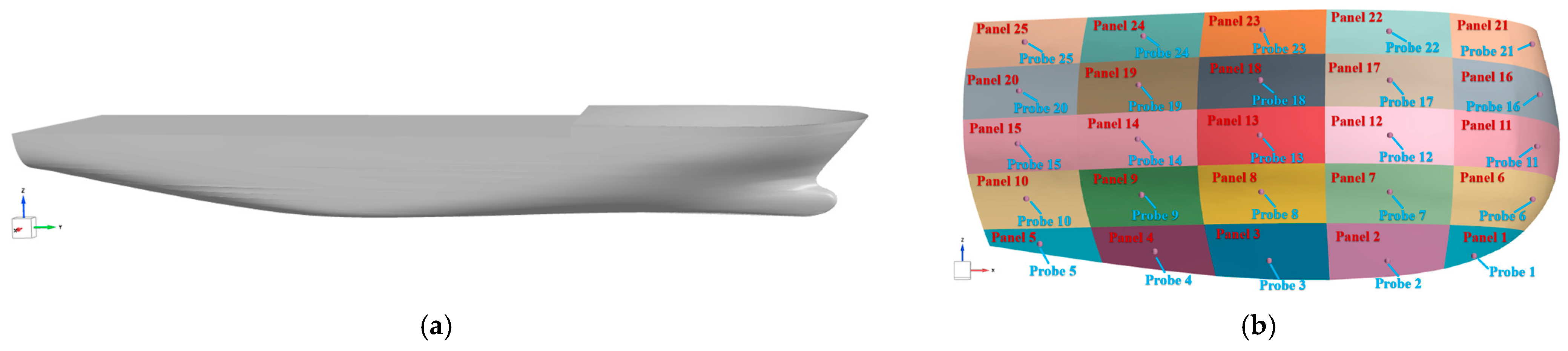
The target vessel considered in this investigation is a representative high-speed slender displacement hull configured with a prominent bulbous bow. To focus on the fundamental hydrodynamic mechanism of wave slamming and viscous scale effects, the bare-hull configuration is adopted as the baseline numerical benchmark, as schematically depicted in Figure 1a. The principal dimensions of the full-scale baseline vessel are defined with a Design Waterline Length (L_WL) and Overall Length (L_OA) of the full-scale ship are 140.0 m and 151.5 m, respectively. The 1:20 scale model serves as the reference case for the numerical simulation. To systematically evaluate scale effects, three additional scale ratios (1:10, 1:15, and 1:50) are modeled based on Froude geometric and dynamic similarity.

Table 1. Principal dimensions and mass characteristics of the baseline full-scale vessel and scaled models.

Parameter	Symbol	Unit	Full Scale (1:1)	Model Scale (1:50)	Model Scale (1:20)	Model Scale (1:15)	Model Scale (1:10)
Scale ratio	α	—	1.0	50.0	20.0	15.0	10.0
Length overall	LOA	m	151.5	3.03	7.575	10.10	15.15
Waterline length	LWL	m	140.0	2.80	7.00	9.333	14.00
Breadth	B	m	18.2	0.364	0.910	1.213	1.820
Depth	D	m	12.8	0.256	0.640	0.853	1.280
Draught	T	m	5.40	0.108	0.270	0.360	0.540
Full-scale design speed	U	kn	16.57	—	—	—	—
Froude number	Fr	—	0.230	0.230	0.230	0.230	0.230
Model speed	Umodel	m/s	—	1.206	1.908	2.203	2.699
Displacement (half ship)	Δ	—	7650 t	61.20 kg	956.25 kg	2266.67 kg	7650.00 kg
Longitudinal CG position	Xg	m	−2.59	−0.052	−0.1295	−0.1727	−0.259
Vertical CG position	Zg	m	7.20	0.144	0.360	0.480	0.720
Radius of gyration (pitch)	Ryy	m	35.00	0.700	1.750	2.333	3.500

Note: Displacement (Δ) is presented in tonnes (t) for the full-scale ship and in kilograms (kg) for the scaled models.

lists the primary geometric and mass characteristics for the full-scale baseline vessel as well as the respective model scales.

A ship-fixed, right-handed Cartesian coordinate system is adopted to define the spatial references, as illustrated in Figure 1. The origin of the coordinate system is positioned at the intersection of the midship section plane, the centerplane, and the still-water level. The positive x-axis points toward the bow, the positive y-axis points toward port, and the positive z-axis points upward.

To evaluate the spatial variations and area-averaging effects of slamming loads, 25 discrete panels are configured across the 3D curved surface of the bulbous bow by subdividing the impact region into a 5 × 5 array along the longitudinal and girthwise directions, as depicted in Figure 1b. The full-scale vessel has an average nominal panel size of about 0.6 m × 0.6 m in the critical keel impact zone after this geometric division. This dimension reflects typical vessel framing arrangements, where the spacing between transverse frames is generally 0.6–0.8 m and that between longitudinal stiffeners is about 0.6–0.7 m. Therefore, each subdivided panel reasonably represents a single unstiffened plate bay between primary structural members, providing a sound basis for equivalent uniform design pressure evaluation. Five main panels (numbered Panel 1 to Panel 5 from forward to aft) are positioned along the keel centerline in the primary impact area. At the same time, 25 local pressure probes are arranged on the surface, with the five centerline probes (Probes 1–5) located at the geometric centers of Panels 1–5 to capture local pressure peaks and spatial gradients.

2.3. Numerical Wave Tank

Regular head waves are generated in the numerical wave tank using the fifth-order Stokes wave formulation to represent steep wave profiles in deep water. The full-scale wave height is set to H = 9.75 m, which corresponds to Sea State 8. Three wavelength-to-ship length ratios are systematically analyzed: λ/L_WL = 1.0, 1.2, 1.4. Based on Froude scaling, the wave parameters and corresponding encounter characteristics for the 1:20 scale model are summarized in

Table 2. Wave and encounter parameters for the 1:20 scale model at different wavelength ratios.

Parameter	Symbol	Unit	λ/LWL = 1.0	λ/LWL = 1.2	λ/LWL = 1.4
Full-scale wavelength	λwave	m	140.0	168.0	196.0
Model-scale wavelength	λm	m	7.00	8.40	9.80
Full-scale wave height	H	m	9.75	9.75	9.75
Model-scale wave height	Hm	m	0.4875	0.4875	0.4875
Full-scale wave period	T	s	9.467	10.370	11.202
Model-scale wave period	Tm	s	2.117	2.319	2.505
Model encounter period	Te	s	1.343	1.519	1.684

.

2.4. Computational Domain and Boundary Conditions

The boundary conditions are defined as:

• Centerplane (y = 0): Symmetry plane boundary.
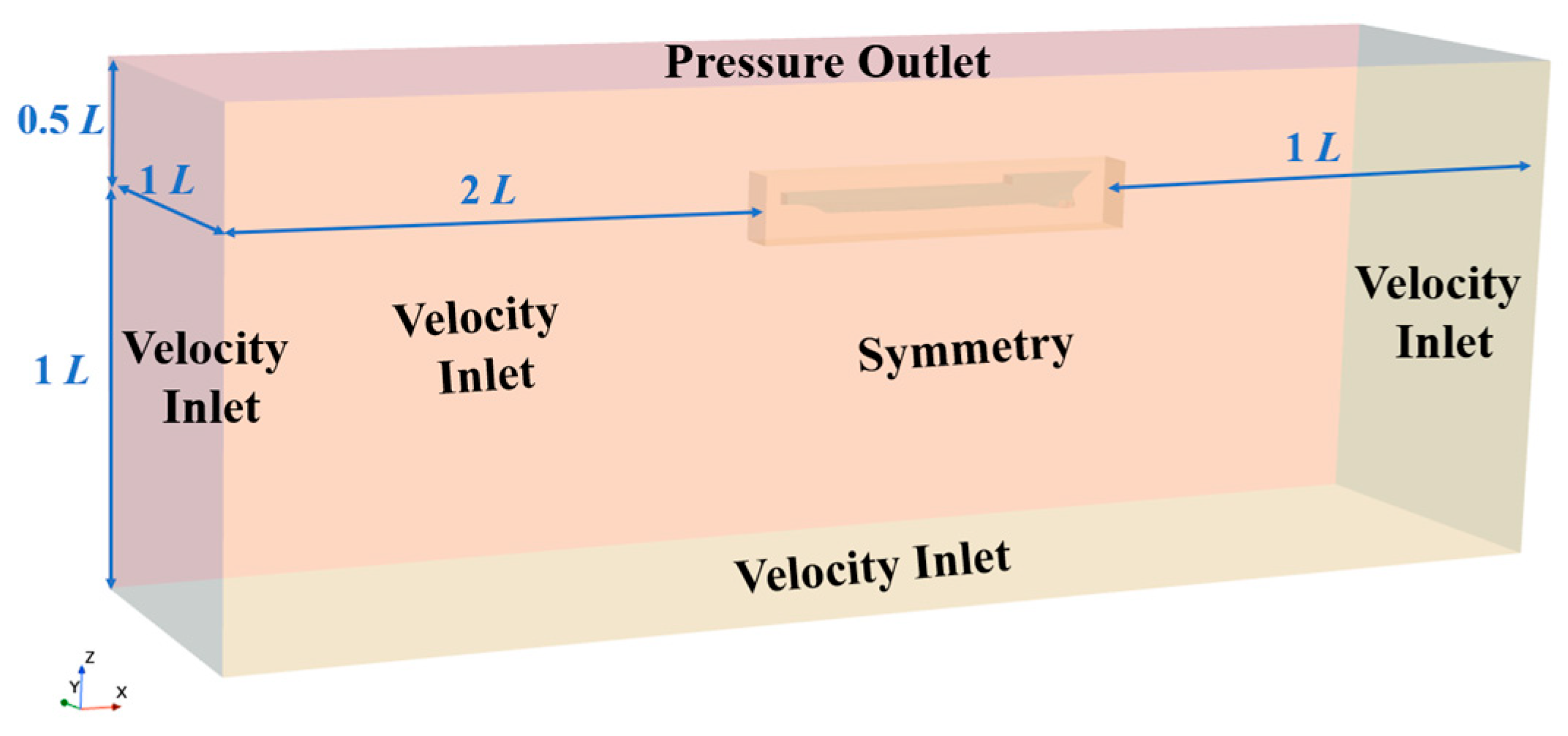
• Top boundary (z = 0.5L_WL): Pressure outlet (representing atmospheric conditions).
• Bottom, Inlet, and Lateral boundaries: Velocity inlets, with fluid velocities and volume fractions defined by the analytical fifth-order Stokes wave kinematics.
• Downstream boundary (x = −2.5L_WL): Pressure outlet coupled with a Wave Forcing relaxation zone. To prevent wave reflections from propagating back into the domain, the Wave Forcing zone is applied with a length of 1.5 times the wavelength (1.5λ_wave), forcing the numerical solution toward the analytical wave profile. The spatial domain and boundary setups of the numerical wave tank are illustrated in Figure 2.

2.5. Mesh and Overset Grid

To accommodate the large-amplitude heave and pitch motions of the ship in waves without grid distortion, numerical discretization is achieved using an overset-grid (also known as chimera grid) topology [36,37]. The computational domain is divided into a stationary background block and a body-fitted overset block that moves rigidly with the hull. Linear interpolation is performed at the overset boundary interface to ensure conservative transfer of mass and momentum between the moving and stationary blocks.

Following the ITTC guidelines for numerical seakeeping and wave loads, the free-surface grid resolution should satisfy three primary criteria: (1) at least 80–120 cells per wavelength, (2) at least 10–20 cells within the wave height range, and (3) a grid aspect ratio (horizontal-to-vertical) at the free surface between 8:1 and 2:1. In the present study, an anisotropic trimmed cell mesh (Cartesian cut-cell grid) with activated grid alignment is utilized to discretize both the background and overset blocks. To minimize numerical wave dissipation during propagation, a local refinement block is established around the free-surface zone using customized anisotropic cell sizes. The vertical grid size at the still-water level is set to Δz = 0.025 m (at the 1:20 model scale), which yields 23 cells within the wave height and approximately 200 cells along the wavelength. The aspect ratio of the free-surface grid is set to Δx:Δz = 4:1 in the longitudinal direction, with a 1:1 ratio between the transverse and longitudinal grid sizes (Δx:Δy:Δz = 4:4:1), which fully satisfies the ITTC recommendations.

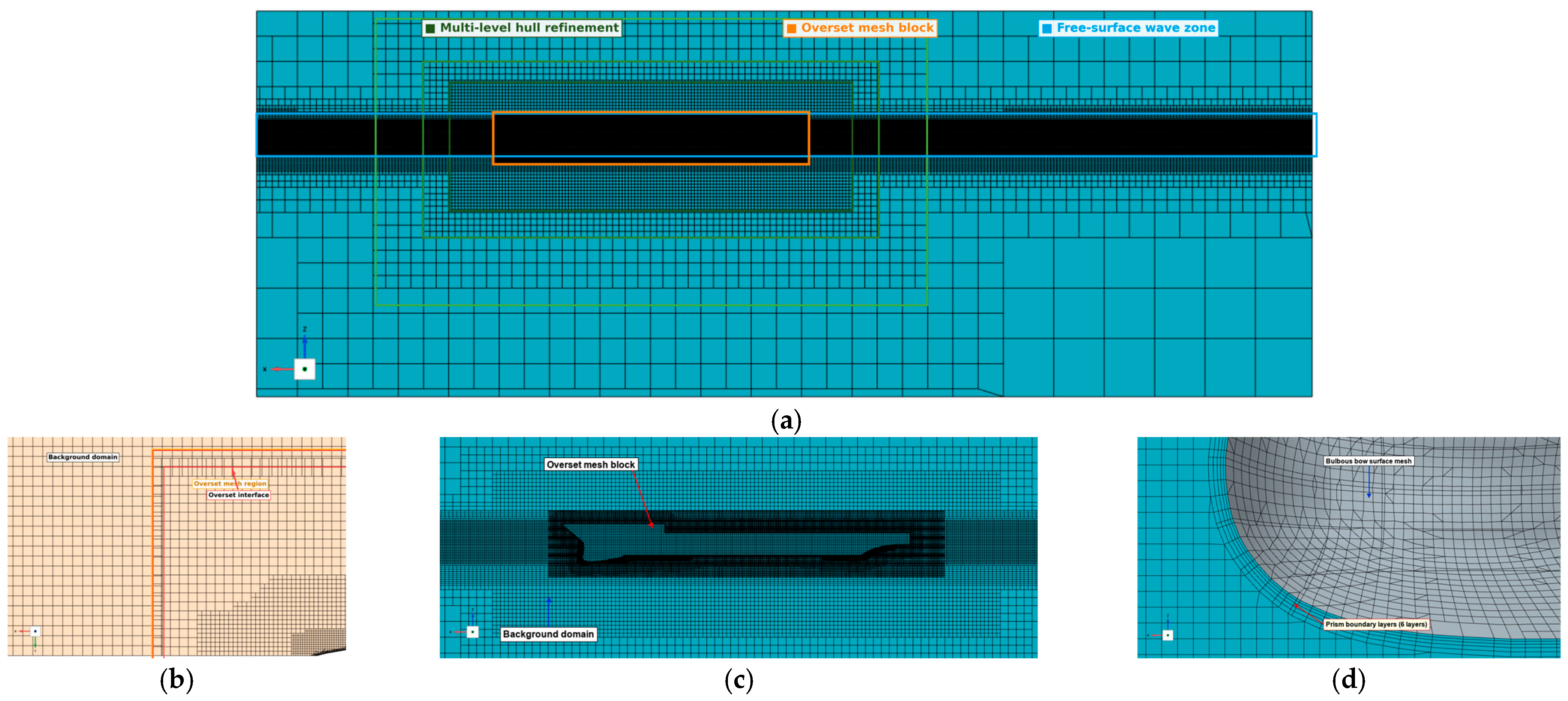
Within the overset block, progressive grid refinement is applied layer-by-layer from the outer boundaries toward the hull surface, with high-density grid refinement applied near the bulbous bow and forward keel to capture the severe flow separation and splash jets during slamming (as illustrated in Figure 3).

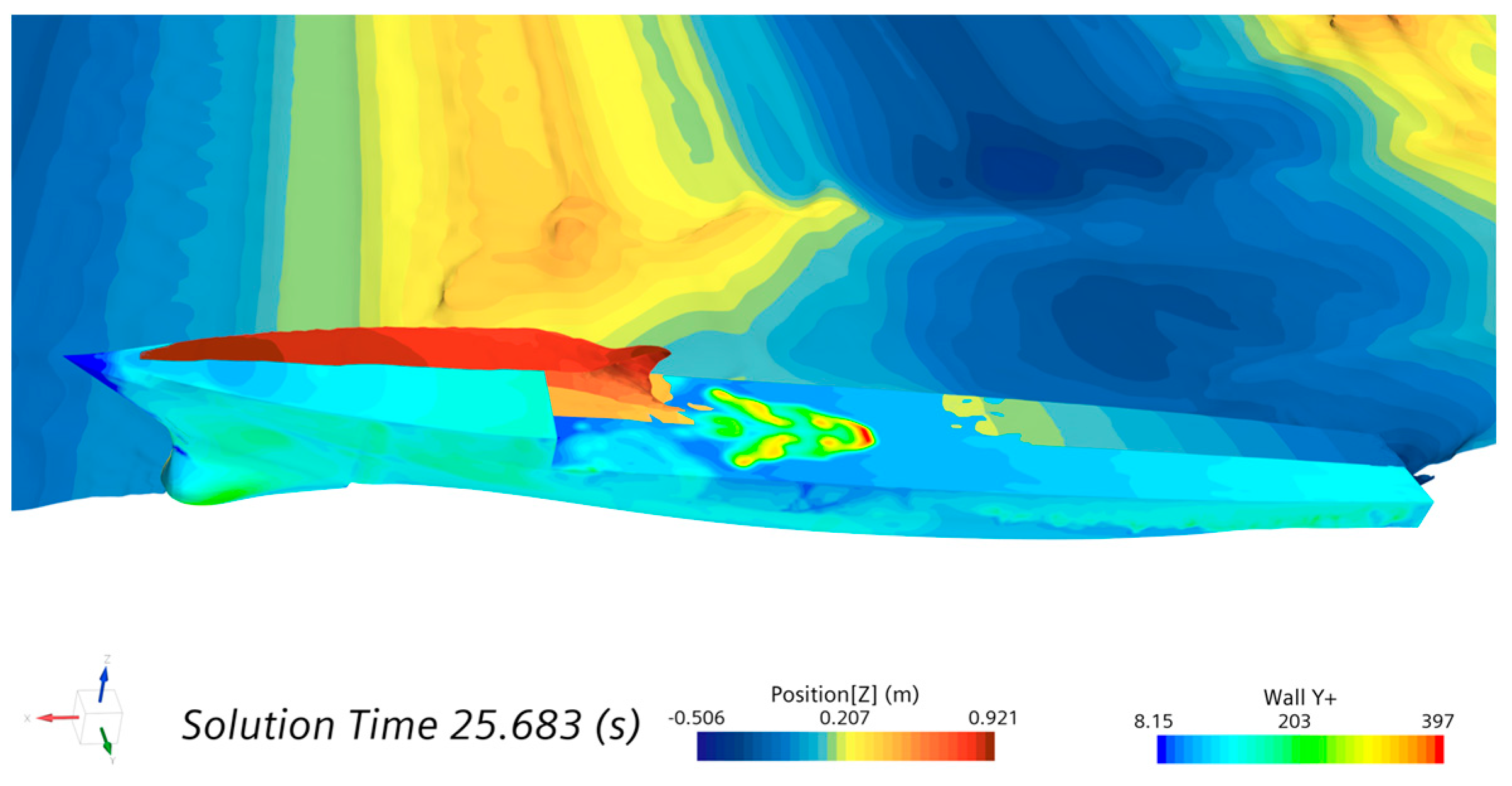
A two-layer all-y⁺ wall treatment was adopted at the vessel’s boundary. The size of the prism layer elements was carefully changed at all test scale ratios. This hybrid wall treatment automatically switches to a low-Reynolds number approach for densely packed grids (y⁺ < 5) and uses standard wall functions where the grid is coarser (y⁺ > 30). In all the scale simulations, the thickness of the first fluid cell was kept to maintain y⁺ within the acceptable operating range for this hybrid model (generally between 5 and 400), and this distribution is shown in Figure 4.

2.6. Rigid Body Motion

The ship motion is solved by the Dynamic Fluid–Body Interaction (DFBI) solver in STAR-CCM+. Only the heave and pitch degrees of freedom are unconstrained, which is consistent with head-sea conditions and the half-ship symmetry assumption. The initial draft is set based on hydrostatic equilibrium, and the motions can develop freely without any other constraints.

3. Numerical Verification

3.1. Wave Calibration

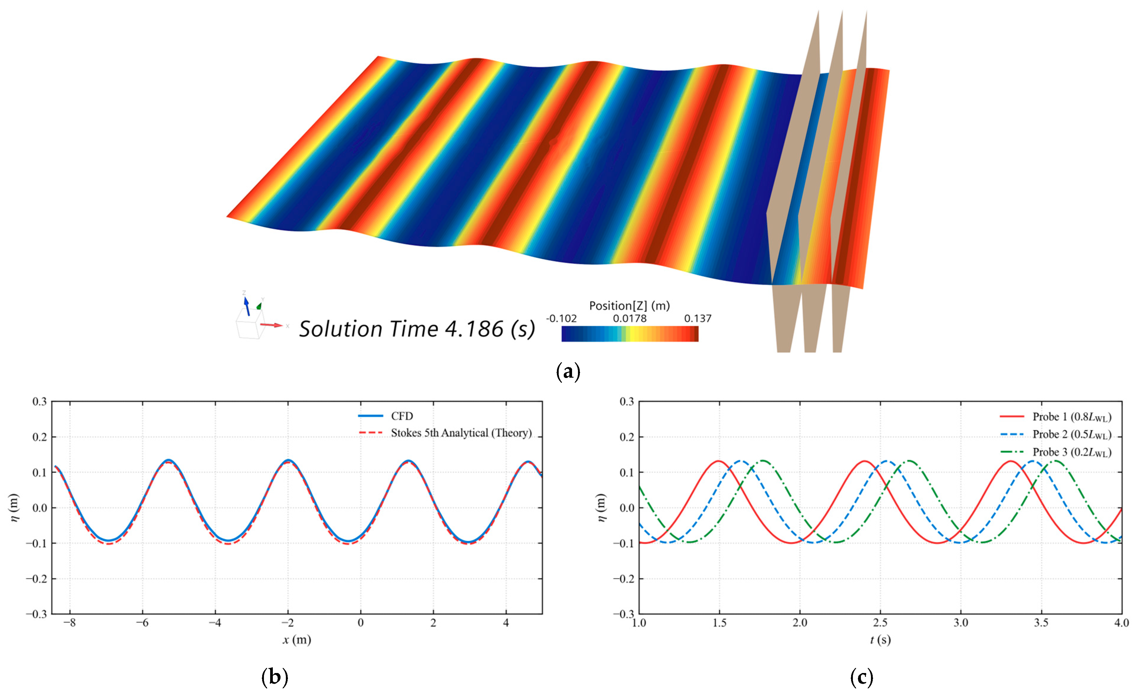
To verify the accuracy and calibrate the numerical wave tank (NWT), wave propagation in an empty tank (without the ship hull) is simulated, as shown in Figure 5.

A typical snapshot of the free-surface wave elevation contour in the numerical wave tank is shown in Figure 5a, and the three vertical planes are the longitudinal measurement positions of the wave probes. Figure 5b is the comparison of the computed spatial wave profile and the analytical solution of the fifth-order Stokes wave. The vertical axis is the wave elevation η (m), and the computed wave profile (with a wave height H = 0.23 m) is compared to the analytical Stokes wave of the same height. The results show that the numerical wave profile is in good agreement with the theoretical Stokes wave at all points in the tank, and there is no phase shift.

Additionally, Figure 5c displays the time histories of the wave elevation η (m) recorded by three virtual wave probes located at 0.8L_WL, 0.5L_WL, and 0.2L_WL from the wave maker (where the wave height is H = 0.23 m). The wave elevations remain highly stable over time, and the wave heights match the target value with a relative error of less than 1.5%, demonstrating that the relaxation-zone-based wave maker and wave dampener successfully prevent wave reflections and numerical damping.

3.2. Wedge Water-Entry

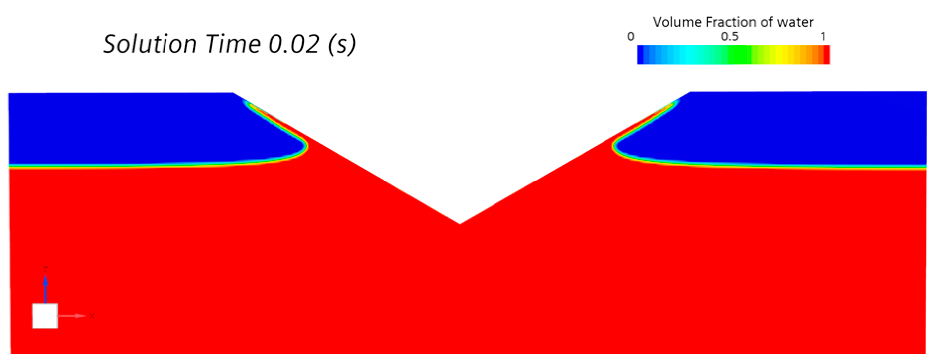
To numerically verify and benchmark the accuracy of the transient pressure resolution and free-surface capturing, a benchmark simulation of a 2D wedge entering calm water is performed. The benchmarking case simulates a symmetric wedge with a deadrise angle of β = 30° entering calm water at a constant downward velocity of V_entry = 6.15 m/s, as shown in Figure 6.

During the slamming process, the pressure along the wedge slope is non-dimensionalized as the pressure coefficient:

$$C_{\mathrm{p}}={\displaystyle \frac{p-p_0}{\frac{1}{2}\rho V_{\mathrm{entry}}^2}}$$

(5)

where p is the local pressure on the wedge surface, p₀ is the atmospheric pressure, ρ is the water density, and V_entry is the constant downward entry velocity. The normalized spatial coordinate along the wedge surface is represented as:

$$s^{*}={\displaystyle \frac{z}{V_{\mathrm{entry}}t}}$$

(6)

where z represents the vertical coordinate relative to the calm water level.

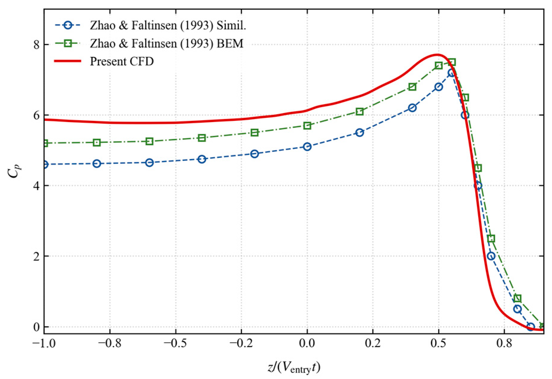
Figure 7 shows the comparison of the computed pressure coefficient along the wedge surface with the similarity solution and Boundary Element Method (BEM) results reported by Zhao and Faltinsen [11]. The present CFD simulation has accurately captured the pressure distribution profile and predicted an apex pressure coefficient of 5.88 (11.5% relative error compared to BEM, due to air compression effects) and a peak pressure coefficient of 7.82 (4.3% relative error compared to BEM).

This localized 11.5% discrepancy observed at the apex can be attributed to simplified numerical and model assumptions: (1) The reference BEM solution is derived under idealized inviscid potential flow theory in a vacuum without air compressibility or viscosity, and minor numerical variations exist even among different theoretical formulations near the sharp vertex [8,11]; and (2) The present multiphase CFD model uses spatial grid averaging near the sharp apex, introducing slight numerical diffusion at the initial contact point. Nevertheless, structural slamming assessments primarily rely on the maximum peak impact pressure and spatial pressure distribution rather than the localized apex point. Given that the maximum peak pressure deviation remains within 4.3% and the overall pressure distribution matches the benchmark curve closely, the numerical setup provides adequate accuracy for predicting violent slamming loads in subsequent bulbous bow analyses.

3.3. Grid Convergence

To enable scale-independent comparison and systematic analysis of seakeeping performance and slamming loads, all physical parameters are presented in dimensionless form. The corresponding expressions (including time, wave elevation, motions, forces, and local pressures) are summarized in

Table 3. Dimensionless expressions of physical quantities.

Physical Quantities	Dimensionless Form	Physical Quantities	Dimensionless Form
Time	$\overline{t}=t\sqrt{g/L}$	Frequency	$\overline{\omega }=\omega \sqrt{L/g}$
Wave elevation	$\overline{\eta }=\eta /{\zeta }_a$	Ship resistance	$\overline{f}=f/\left(0.5\rho U^{2}S\right)$
Heave	$\overline{z}=z/{\zeta }_a$	Pitch	$\overline{\theta }=\theta /\left(k{\zeta }_a\right)$
Acceleration	$\overline{a}=a/g$	Vertical bending moment (VBM)	$\overline{M}=M/\left(\rho g{L}^{2}B{\zeta }_a\right)$
Vertical shearing force (VSF)	$\overline{F}=F/\left(\rho \mathit{gLB}{\zeta }_a\right)$	Impact pressure	$C_p=P/\left(0.5\rho U^2\right)$

.

In this study, the variables presented in Table 3 are defined as follows: t, z, θ, and p represent the physical time, heave displacement, pitch angle, and local slamming pressure, respectively. Additionally, F_z and M_y denote the vertical slamming force and pitch moment. The geometric and environmental parameters include the ship waterline length L, gravitational acceleration g, fluid density ρ, regular wave amplitude ζ_a, and wave number k (where k = 2π/λ). The overbar notation (e.g., $\overline{t}$, $\overline{z}$, $\overline{\theta }$) explicitly denotes the corresponding dimensionless quantities.

3.3.1. Ship Motion Responses

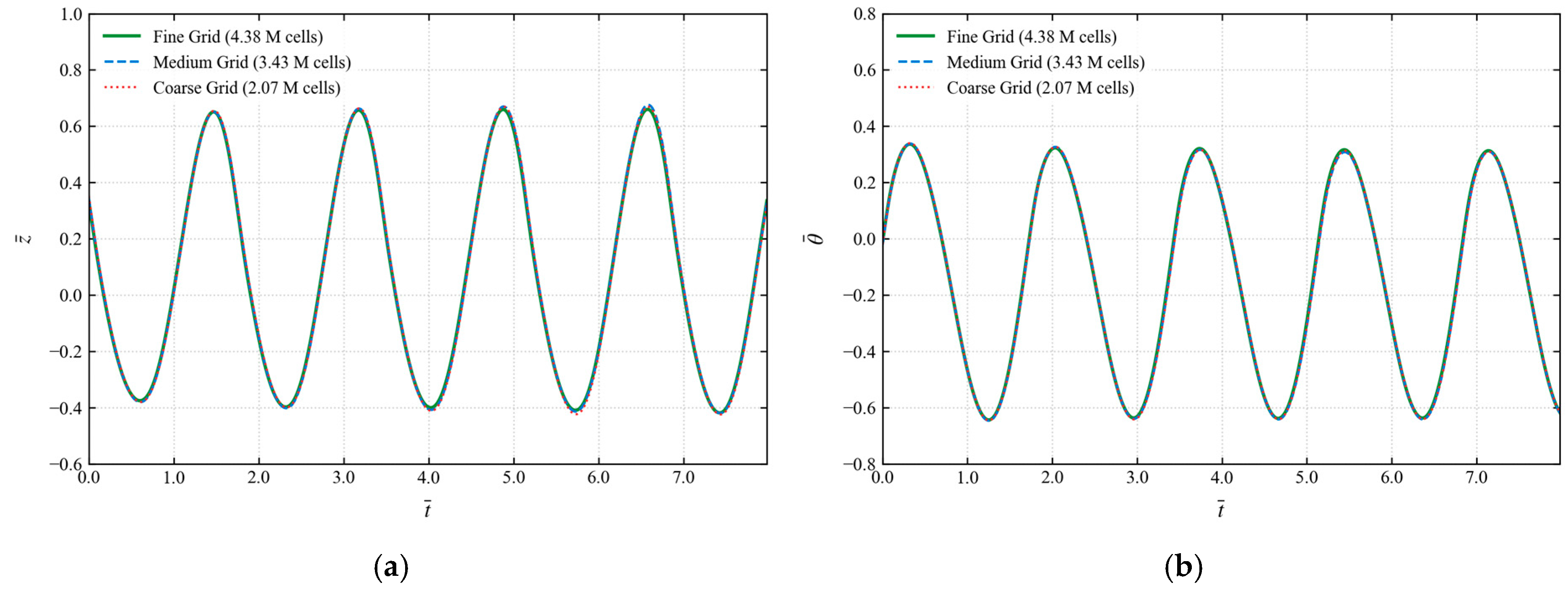
To verify grid independence and quantify numerical uncertainty, a systematic study is conducted following the ITTC guidelines. Three grids are generated: Coarse (Grid 1, 2.07 × 10⁶ cells), Medium (Grid 2, 3.43 × 10⁶ cells), and Fine (Grid 3, 4.38 × 10⁶ cells), as shown in Figure 8.

Under the wave encounter condition at λ/L_WL = 1.0, the peak motion amplitudes are extracted, as summarized in

Table 4. Convergence parameters of grid independence study.

Key Variables	Coarse (N1)	Medium (N2)	Fine (N3)	Convergence Ratio (R)	Apparent Order (pG)	GCIfine
Heave amplitude (m)	0.0763	0.0772	0.0776	0.444 (monotonic)	6.44	0.93%
Pitch amplitude (deg)	3.90	3.93	3.95	0.667 (monotonic)	3.22	2.11%

.

The grid convergence analysis is conducted in accordance with ITTC recommended procedures and Roache’s Grid Convergence Index (GCI) methodology. The grid convergence ratio is defined as:

$$R={\displaystyle \frac{{\epsilon }_{32}}{{\epsilon }_{21}}}$$

(7)

where ${\epsilon }_{21}=S_2-S_1$ and ${\epsilon }_{32}=S_3-S_2$ represent the solution differences between medium-coarse and fine-medium grids, with S₁, S₂, and S₃ denoting the coarse, medium, and fine grid solutions, respectively. The apparent order of convergence p_G and the fine-grid numerical uncertainty GCI_fine (with a factor of safety F_s = 1.25) are evaluated as:

$$P_G={\displaystyle \frac{\ln |{\epsilon }_{21}/{\epsilon }_{32}|}{\ln r_{\mathrm{avg}}}}$$

(8)

$$GC{I}_{\mathrm{fine}}={\displaystyle \frac{F_s|(S_3-S_2)/S_3|}{r_{32}^{p_G}-1}}\times 100\%$$

(9)

where $r_{a\mathrm{v}\mathrm{g}}=\left(r_{21}+r_{32}\right)/2$ is the average refinement ratio. As summarized in Table 4, the convergence ratios R for heave and pitch are 0.444 and 0.667 (0 < R < 1), confirming monotonic convergence. The apparent orders of convergence are calculated as p_G = 6.44 for heave and p_G = 3.22 for pitch, resulting in fine-grid discretization uncertainties of GCI_fine = 0.93% and GCI_fine = 2.11%, respectively. The global motion responses exhibit excellent agreement across the three grids, as shown in Figure 9, confirming high spatial convergence for rigid-body motions.

3.3.2. Local Slamming Pressures

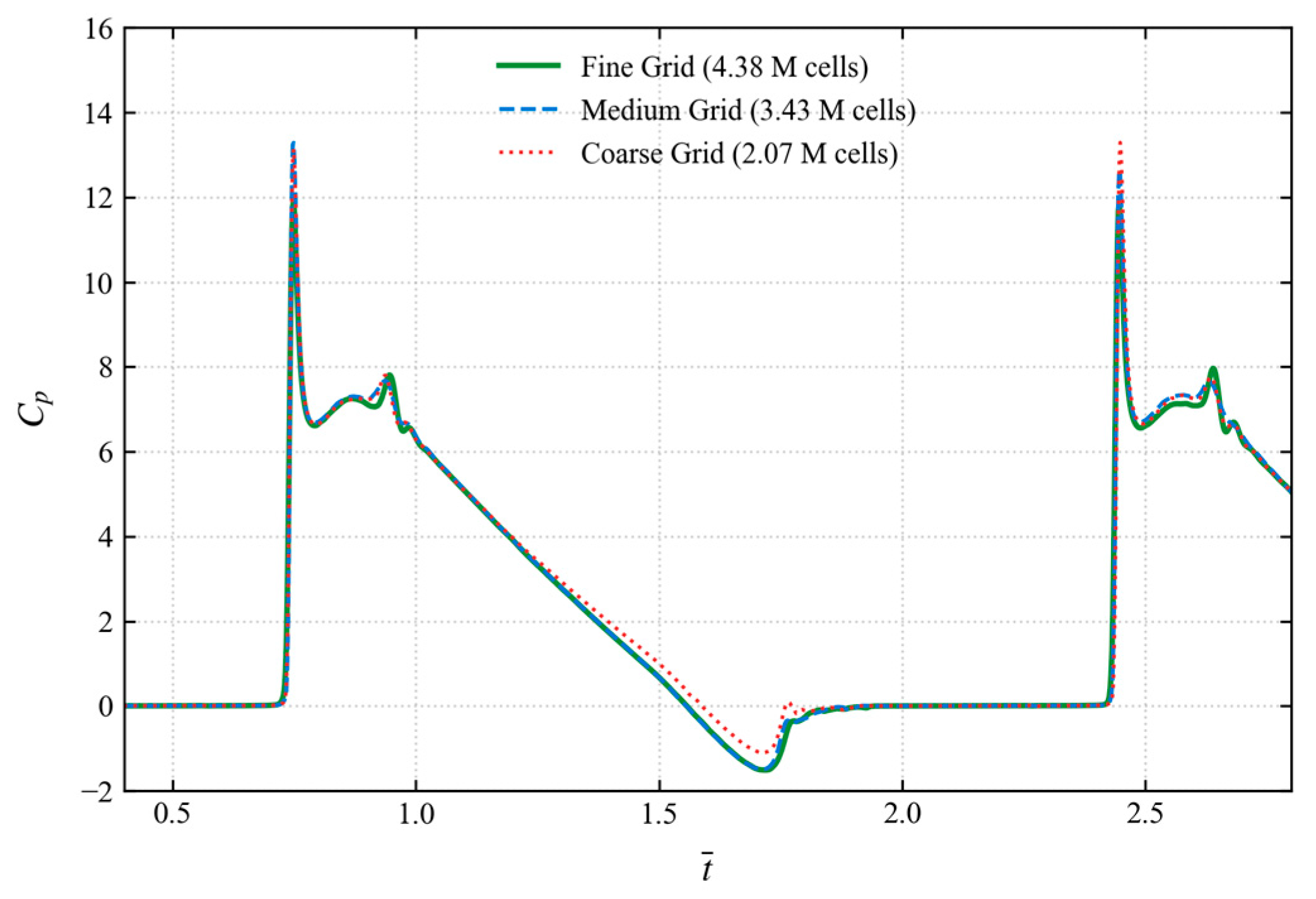
To find out how sensitive the local force is to grid size, the pressure coefficient (C_p) histories at Probe 1 are shown for coarse, medium and fine meshes. As shown in Figure 10, the pressure profiles are aligned over a single wave encounter cycle. The peak C_p values for the coarse, medium and fine meshes are 13.14, 13.42 and 11.90 respectively.

Unlike integrated global motions, highly localized point pressures are sensitive to local cell sizing due to steep spatial pressure gradients and transient spray jet detachment. The peak C_p exhibits an 11.3% reduction from the medium grid (13.42) to the fine grid (11.90), reflecting the enhanced resolution of fine-scale flow separation and local interface curvature in the fine mesh. Nevertheless, the temporal pulse duration (τ), the steep pressure rise rate, and the subsequent negative suction phase during bow emergence [1,4] show strong consistency across the medium and fine grids. The evaluated GCI_fine for the localized peak slamming pressure at Probe 1 is 4.31%, indicating low spatial discretization uncertainty. Considering that the medium grid achieves low numerical uncertainty (GCI_fine ≤ 2.11% for global motions and GCI_fine = 4.31% for localized peak pressure) and captures the transient slamming characteristics with acceptable engineering accuracy while saving approximately 45% of computational resources compared to the fine grid, the Medium grid configuration (3.43 M cells) is selected as the baseline mesh for all subsequent multi-scale comparative studies.

3.4. Time-Step Convergence

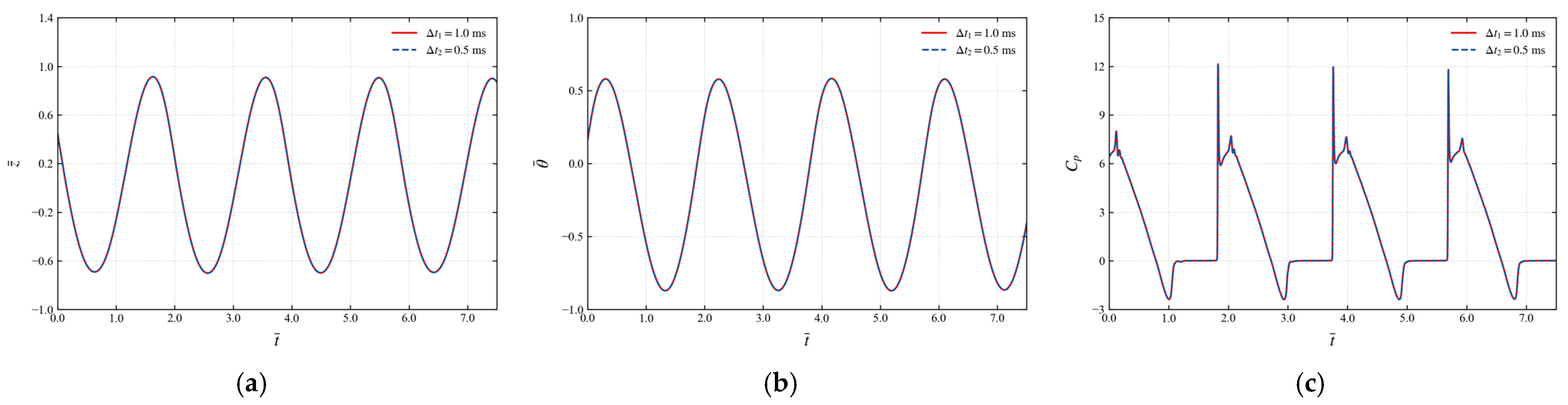
To evaluate the influence of the time step on slamming load prediction, a sensitivity study is carried out under the critical wave condition (λ/L_WL = 1.2) at a 1:50 scale. The baseline time step (Time Step-1) is set to Δt₁ = 0.001 s (i.e., 1.0 ms), and the fine time step (Time Step-2) is set to Δt₂ = 0.5 ms. The global motions show a maximum deviation of 1.5% for heave and 0.4% for pitch, confirming high time-step independence for global ship motions, as shown in Figure 11a,b.

The peak pressure coefficient C_p at Probe 1 shows negligible difference between the two time steps (remaining at approximately 12.14), reflecting excellent time-step convergence of the transient slamming pressure spikes, as shown in Figure 11c. Since the baseline time step accurately captures both the global motions and local peak loads while saving 50% of the computational expense, it is adopted as the baseline time step for the parametric studies.

For temporal resolution in the multi-scale simulations, both global wave encounter periodicity and local slamming pulse duration are used to determine the computational time step. Standard ITTC guidelines and established numerical practices for ship-wave interactions [38] recommend at least 200 to 400 time steps per wave encounter period (T_e). For the 1:50 model scale, with a baseline time step of Δt = 0.001 s, about 960 time steps are obtained per encounter period (T_e ≈ 0.9 s). For the larger-scale models (α = 1:20, 1:15, and 1:10), where the wave encounter period reaches T_e ≈ 2 s ($T_{\mathrm{e}}\propto \sqrt{\lambda }$), a time step of Δt = 0.005 s provides approximately 430 time steps per cycle, strictly satisfying the ITTC temporal criterion across all simulated scales.

In terms of localized slamming, because the hydrodynamic impact duration scales with hull size ($\tau \propto \sqrt{\lambda }$), the transient pressure pulse duration increases from τ ≈ 25 ms at 1:50 scale to τ ≈ 60 ms at 1:10 scale. Consequently, the selected time steps ensure that the sharp impact pressure spike is resolved with 12 to 25 computational time steps across the peak duration for all simulated scales, accurately capturing the rapid pressure rise and peak magnitude while maintaining numerical stability and computational efficiency.

4. Motions and Slamming Pressures

4.1. Effect of Wavelength

Numerical simulations are performed at a model speed of U = 1.908 m/s in regular head waves of height H_model = 0.4875 m (corresponding to a full-scale wave height of H = 9.75 m) across λ/L_WL = 1.0, 1.2, 1.4. To eliminate startup transients and establish steady-state periodic conditions, peak motion amplitudes and local pressure values are systematically extracted over the 3rd–5th stabilized encounter cycles.

To clarify which wavelength governs the most severe loading, the wave encounter period T_e is evaluated for each condition. In head seas, the encounter frequency is:

$${\omega }_{\mathrm{e}}={\omega }_{\mathrm{w}}+k_{\mathrm{w}}U,\hspace{1em}\hspace{1em}{k}_{\mathrm{w}}={\omega }_{\mathrm{w}}^2/g,\hspace{1em}\hspace{1em}{\omega }_{\mathrm{w}}=\sqrt{{\displaystyle \frac{2\pi g}{{\lambda }_{\mathrm{wave}}}}}\hspace{1em}\hspace{1em}$$

(10)

where ω_w is the intrinsic wave frequency, k_w is the wavenumber, and U is the forward speed. Because the vessel advances into head waves, the encounter frequency ω_e is significantly higher than the intrinsic wave frequency ω_w, resulting in a reduced encounter period T_e. The seakeeping characteristics, including the wave parameters and stabilized peak heave and pitch motion amplitudes, are summarized in

Table 5. Encounter parameters, non-dimensional motion amplitudes, and peak panel pressure coefficients for the three wavelength conditions (1:20 scale).

λ/LWL	Te,model (s)	Te,full (s)	ωe,full (rad/s)	$\overline{\mathit{z}}$	$\overline{\mathit{\theta }}$	Cp,max Panel 1
1.0	1.343	6.00	1.047	0.62	0.44	9.47
1.2	1.519	6.79	0.925	0.88	0.70	10.97
1.4	1.684	7.53	0.835	0.88	0.88	9.12

.

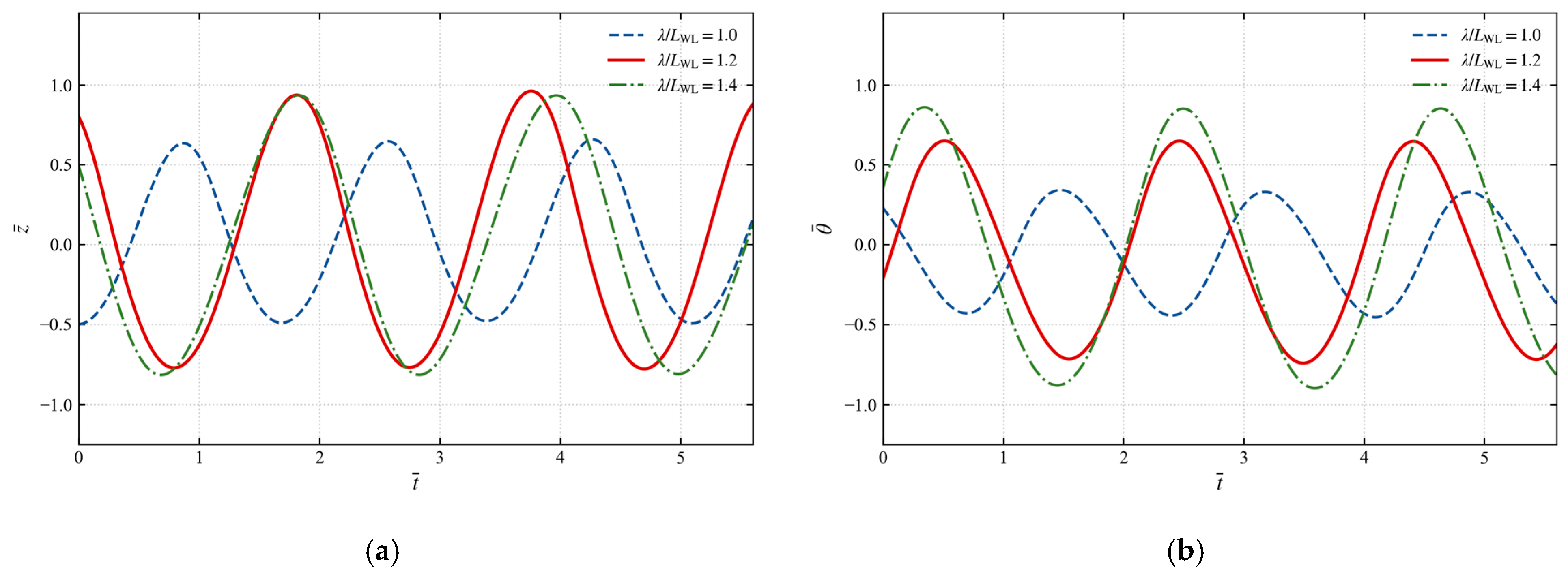
The time histories of the non-dimensional heave and pitch motions under the three wavelength conditions are shown in Figure 12a,b.

Among the three wave conditions tested, the wavelength ratio λ/L_WL = 1.2 had the highest slamming pressure coefficient (C_p,max = 10.97 at Panel 1). Although the non-dimensional heave amplitude plateaus between λ/L_WL = 1.2 and 1.4, and the pitch motion reaches its maximum at λ/L_WL = 1.4, the peak slamming load is still relatively concentrated at λ/L_WL = 1.2. This behavior can be caused by seakeeping phase superposition. At λ/L_WL = 1.2, because of a phase difference between the coupled heave-pitch response and the incoming wave, there is a maximum relative vertical velocity at the bow. This phase alignment causes the bow to lift high up before smashing back into the water at a high relative speed. Therefore, although longer waves induce larger pitch amplitudes, the resulting extreme slamming pressures are so high that λ/L_WL = 1.2 is considered a critical structural case for the sea state under consideration. Therefore, this particular case served as the foundation for the following parametric scale-effect analyses.

This wavelength range covers the typical resonance region for surface vessels in head seas, and the peak response wavelength (λ/L_WL = 1.2) has been observed in previous numerical and experimental studies [1,13].

The maximum physical slamming pressure in Pa and its corresponding pressure coefficient C_p for key bottom panels and point probes of the 1:20 scale model under different wavelength ratios are shown in

Table 6. Maximum pressure peak values for the 1:20 model at different wavelength ratios.

Location	λ/LWL = 1.0		λ/LWL = 1.2		λ/LWL = 1.4
	p (Pa)	Cp	p (Pa)	Cp	p (Pa)	Cp
Panel 1	19,568	10.77	19,924	10.97	11,270	6.20
Panel 2	18,275	10.06	19,179	10.56	10,047	5.53
Panel 3	13,377	7.36	16,718	9.20	8486	4.67
Panel 4	9275	5.10	16,504	9.08	8021	4.41
Panel 5	8427	4.64	12,975	7.14	5658	3.11
Probe 1	20,714	11.40	22,465	12.36	12,994	7.15
Probe 2	21,146	11.64	22,176	12.21	11,646	6.41
Probe 3	18,163	10.00	18,493	10.18	10,095	5.56
Probe 4	10,455	5.75	17,036	9.38	9501	5.23
Probe 5	7675	4.22	12,045	6.63	6165	3.39

.

4.2. Spatiotemporal Pressure Distribution

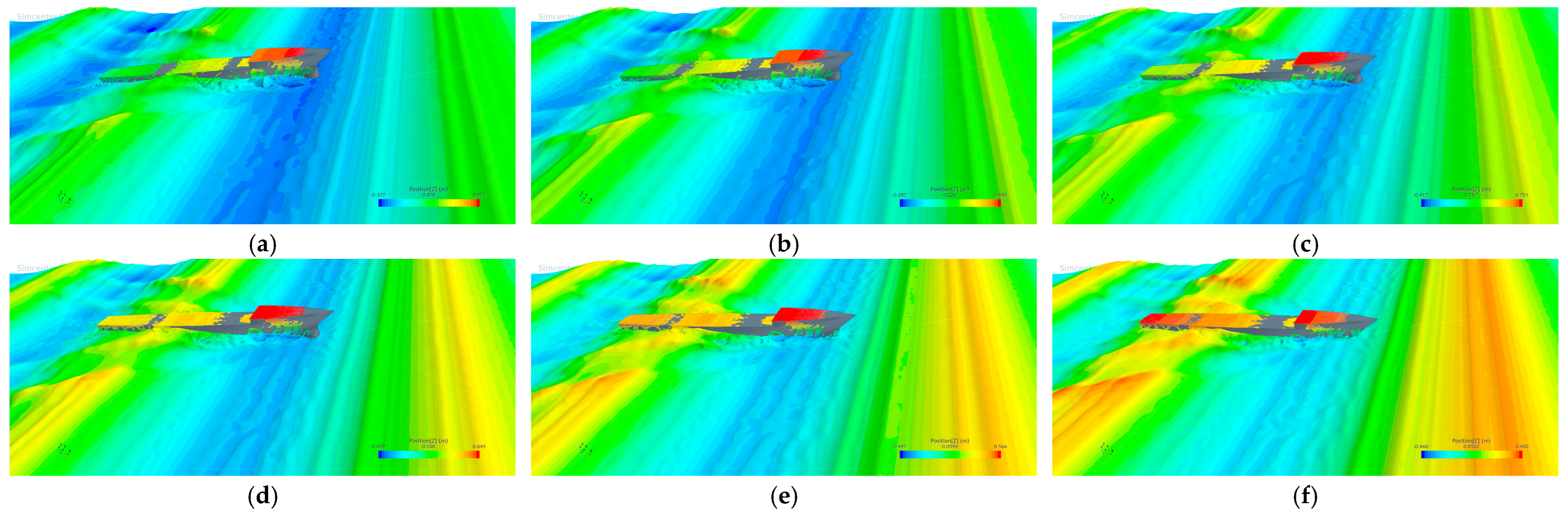
To study the physical reason for the water-impact phenomenon, the space-time distribution of slamming pressure during a representative resonant water-entry period (t = 19.60–19.80 s, at 1:20 model scale) is analyzed. Figure 13 shows the free-surface elevation contours.

4.2.1. Vertical Distribution

As shown by the free-surface elevation contours in Figure 13, the vertical distribution of the slamming pressure is not uniform. This non-uniformity arises from the hull’s geometry and the sequential nature of the water-entry process. The bottom panels at the keel centreline (Panel 1 to Panel 5) are exposed to the largest slamming forces and have a sudden pressure increase. The large load results from a near-horizontal bottom at the moment of striking the free surface during bow submergence. The side panels of the bulbous bow experience relatively small slamming forces. As the hull surface in these areas is almost vertical, the water will run along the side wall rather than hitting it directly. Later in the entry stage, wave run-up and splash-jet formation along the upper bow curvature cause a secondary pressure increase on the upper flare panels. As the keel centreline is the main area of high stress, the following quantitative analyses will be carried out only on these centreline panels and point probes.

4.2.2. Longitudinal Distribution

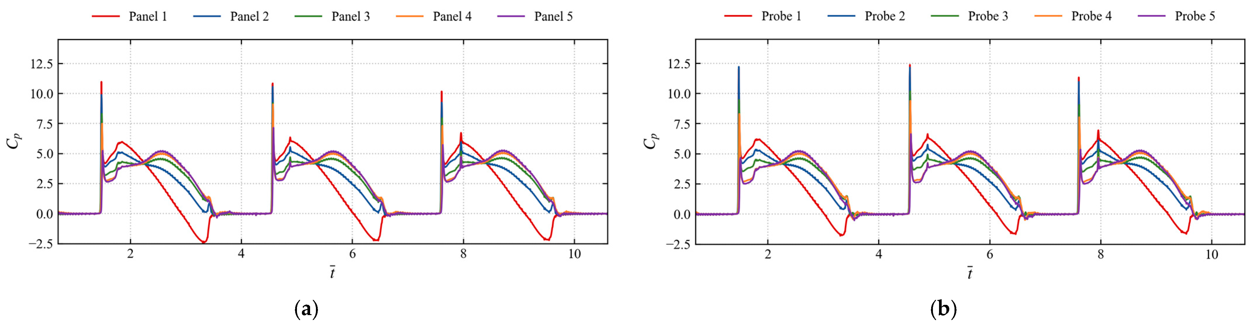
The pressure at the keel line is relatively high near the front and gradually decreases towards the back; specifically, from Panel 1 to Panel 5, this pressure is decreasing. This decrease happens because the vertical velocity of the hull relative to the waves is relatively high at the front end due to the combined effect of pitching and heaving. As shown in the time-history plots of C_p in Figure 14, a sequential propagation of impact pressures occurs in both panel-averaged (Figure 14a) and point-probe (Figure 14b) measurements. It begins at the front and moves back, and there is a relatively long time lag. This phase lag reflects the gradual wetting of the keel as the bow dips into the incoming wave crest, a behavior that agrees well with analytical water-entry models [9,10].

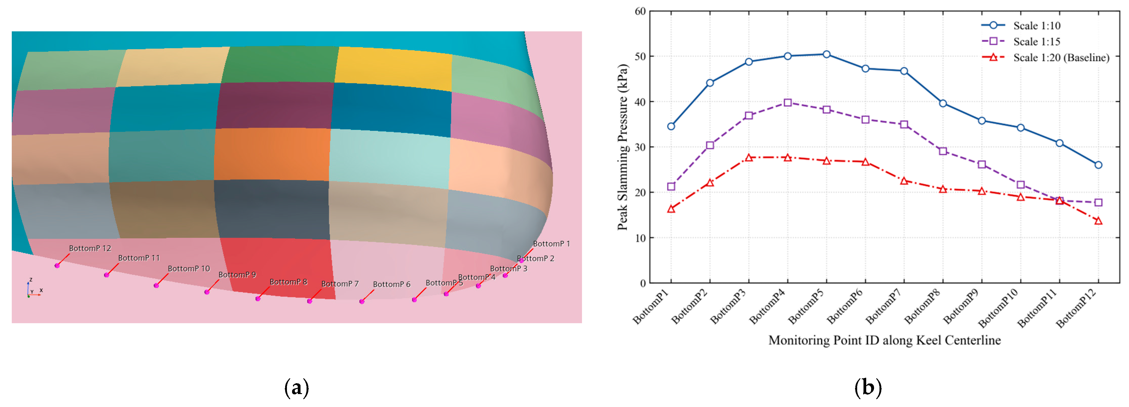
To provide a high-resolution longitudinal profile of the impact pressures,

Table 7. Maximum slamming pressures along the keel centerline points (BottomP1 to BottomP12) across three scale ratios.

Probe ID	Panel ID	1:20 Scale (Pa)	1:15 Scale (Pa)	1:10 Scale (Pa)
BottomP1	Panel 2	16,383	21,222	34,534
BottomP2	Panel 1	22,116	30,389	44,106
BottomP3	Panel 1	27,668	36,926	48,792
BottomP4	Panel 1	27,696	39,752	50,040
BottomP5	Panel 2	26,958	38,244	50,428
BottomP6	Panel 2	26,725	36,032	47,259
BottomP7	Panel 3	22,545	34,956	46,770
BottomP8	Panel 3	20,690	29,025	39,620
BottomP9	Panel 4	20,280	26,126	35,780
BottomP10	Panel 4	19,046	21,679	34,245
BottomP11	Panel 5	19,015	18,203	31,120
BottomP12	Panel 5	13,760	17,736	26,031

lists the maximum slamming pressures recorded at twelve closely spaced points (BottomP1 to BottomP12) along the keel centerline for the 1:20, 1:15, and 1:10 scale models. The spatial layout and longitudinal distribution of these bottom monitoring points along the centerline of the bulbous bow are shown in Figure 15.

The pressures systematically decay from the forward extremity (BottomP4 reaches 27,696 Pa at 1:20 scale) toward the sternward section (BottomP12 is 13,760 Pa at 1:20 scale), which corresponds to the progressive wetting and pitching entry process. This high-resolution distribution demonstrates that the critical impact load is concentrated within the forward 20% of the ship length (from the forward extremity to BottomP5).

To ensure consistency across all multi-scale comparisons, the scale effect analysis in Section 5 is systematically conducted on the five primary benchmark locations (Locations 1, 6, 11, 16, and 21), which are monitored across all four scale ratios. The additional high-resolution points (BottomP1 to BottomP12) serve as supplementary spatial measurements to detail the localized keel-line pressure gradients at intermediate scales, and were not deployed in the 1:50 scale model to optimize computational data storage.

4.2.3. Water-Exit Suction

After the first peak of slamming, a sub-atmospheric negative pressure phase (C_p < 0) occurs at all keel-centreline probes during the bow water-exit stage. As the ship’s bow rises sharply relative to the wave, there is a discrepancy in the downward inertia of the displaced fluid at the solid-fluid interface. This discrepancy causes a lower pressure in that area compared with the atmospheric level, which produces a suction effect. Since the minimum gauge pressure observed in the simulation remains well above the water vapor pressure limit, no cavitation occurs. Therefore, these negative gauge pressures correctly represent the physical hydrodynamic suction acting on the hull during the water-exit phase. Although neglecting the cavitation limit may lead to a slight overprediction of the suction magnitude during exit, this has no effect on the positive slamming peaks during water entry, which govern the structural design loads [2,28]. This suction phenomenon is physically consistent with analytical water-exit theories describing the rapid contraction of the wetted surface [10,11,39] and has been reported in experimental and numerical seakeeping tests [1,4].

4.3. Panel and Probe Pressures

To evaluate the spatial averaging effect on slamming load prediction,

Table 8. Comparison of peak local pressures (Probe) and area-averaged pressures (Panel) across multiple scale ratios.

Location	1:50 Model		1:20 Model		1:15 Model		1:10 Model
	p (Pa)	Cp	p (Pa)	Cp	p (Pa)	Cp	p (Pa)	Cp
Panel 1 (Average)	6739	9.28	19,924	10.97	27,433	11.33	43,635	12.00
Probe 1 (Local)	7471	10.29	22,465	12.36	31,670	13.07	46,853	12.89
Panel 2 (Average)	7123	9.81	19,179	10.56	25,426	10.50	40,230	11.07
Probe 2 (Local)	7907	10.89	22,176	12.21	30,090	12.42	46,179	12.70
Panel 3 (Average)	6283	8.66	16,718	9.20	22,136	9.14	33,790	9.29
Probe 3 (Local)	6753	9.30	18,493	10.18	25,857	10.67	38,149	10.49
Panel 4 (Average)	4904	6.76	16,504	9.08	20,029	8.27	29,273	8.06
Probe 4 (Local)	5324	7.33	17,036	9.38	22,181	9.16	30,619	8.43
Panel 5 (Average)	3862	5.32	12,975	7.14	15,197	6.27	25,078	6.90
Probe 5 (Local)	3684	5.08	12,045	6.63	15,520	6.41	28,370	7.81

compares the peak local pressures recorded by point probes with the corresponding area-averaged pressures over the structural panels across multiple scale ratios.

Table 8 demonstrates that integrating pressure over a panel area yields peak C_p values that are uniformly lower than those recorded by single-point probes in the critical slamming regions (Panels 1 through 4).

At a 1:20 scale, the peak area-averaged pressure coefficient decreases by 11.2% (Panel 1), 13.5% (Panel 2), 9.6% (Panel 3) and 3.2% (Panel 4) after area averaging. The entire region shows a reduction in the magnitude of the severe pressure spike near the front tip of the bulbous bow. On the other hand, further aft at Panel 5, the measurements are in good agreement; in fact, the panel shows a slightly higher load (+7.7%) than the point probe due to flow separation and a more uniform local pressure field. A substantial decrease in the forward zone indicates that, although localized point probes record high instantaneous pressure peaks, the surrounding structural panel naturally averages out this concentrated load across its entire surface. In ship structural assessment, point pressures and area-averaged panel loads serve complementary engineering purposes: localized point pressure peaks are essential for evaluating localized plating denting and fatigue damage near welded details, whereas area-averaged panel pressures provide more realistic, non-overconservative boundary conditions for plate yielding checks and finite-element structural analysis [4,28].

4.4. Slamming Impulse

To analyze the dynamic response of a structure under slamming, both the maximum magnitude of the load and the duration of the load need to be considered. A dimensionless slamming impulse I* is defined as the total momentum transfer per unit area:

$$I^{*}=C_{\mathrm{p},\max }\times {\tau }_{\mathrm{rise}}^{\prime }$$

(11)

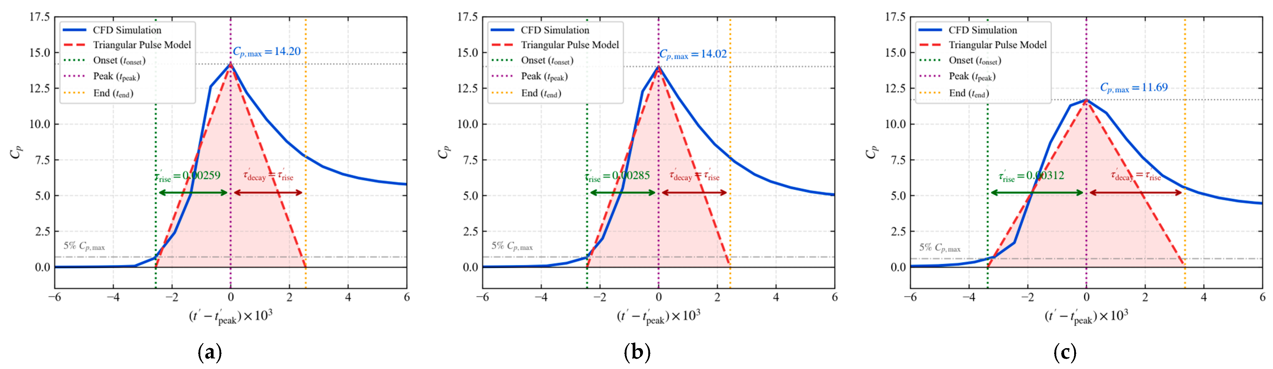
where ${\tau }_{\mathrm{r}\mathrm{i}\mathrm{s}\mathrm{e}}^{\prime }={\tau }_{\mathrm{r}\mathrm{i}\mathrm{s}\mathrm{e}}U/L_{WL}$ is defined as the dimensionless pressure rise time, with τ_rise measured from the initial onset of rapid pressure increase (5% C_p,max threshold) to the instantaneous peak ($t_{\mathrm{p}\mathrm{e}\mathrm{a}\mathrm{k}}-t_{\mathrm{o}\mathrm{n}\mathrm{s}\mathrm{e}\mathrm{t}}$). This formulation is mathematically equivalent to the total area under an idealized symmetric triangular pressure pulse with a total duration of ${2\tau }_{\mathrm{r}\mathrm{i}\mathrm{s}\mathrm{e}}^{\prime }({\tau }_{\mathrm{d}\mathrm{e}\mathrm{c}\mathrm{a}\mathrm{y}}^{\prime }={\tau }_{\mathrm{r}\mathrm{i}\mathrm{s}\mathrm{e}}^{\prime }$), as illustrated in Figure 16.

In physical ship slamming events, the instantaneous CFD pressure history exhibits an asymmetric profile across the impact window. During initial water entry ($t<t_{\mathrm{p}\mathrm{e}\mathrm{a}\mathrm{k}}$), pressure rises sharply as the bow surface penetrates the wave, showing strong agreement with the linear ramp of the triangular model. After the peak ($t>t_{\mathrm{p}\mathrm{e}\mathrm{a}\mathrm{k}}$), the pressure decays gradually rather than dropping symmetrically to zero, producing an extended unloading tail as fluid spreads over the curved bulbous bow before reaching hydrostatic submergence.

As compared in

Table 9. Dimensionless slamming impulse I* at key keel locations (1:20 scale, λ/L_WL = 1.2).

Parameter	Probe 1 (Bow Tip)	Probe 2 (Mid-Forward)	Probe 3 (Mid Keel)
Cp,max	12.36	12.21	10.18
${\tau }_{\mathrm{r}\mathrm{i}\mathrm{s}\mathrm{e}}^{\prime }$	0.00259	0.00285	0.00312
$I_{t\mathrm{r}\mathrm{i}}^{*}$	0.0320	0.0348	0.0318
$I_{\mathrm{i}\mathrm{n}\mathrm{t}}^{*}$	0.0441	0.0432	0.0432
$I_{t\mathrm{r}\mathrm{i}}^{*}/I_{\mathrm{i}\mathrm{n}\mathrm{t}}^{*}$(%)	72.6%	80.6%	73.6%

and Figure 16, the idealized triangular pulse bounds the primary dynamic impact phase well, capturing approximately 72.6% to 80.6% of the hydrodynamic impulse over the primary pulse interval. The remaining 20% to 27% difference is attributed to the extended post-peak unloading tail. This symmetric triangular pulse idealization represents a classical engineering approach widely adopted in classification society rules and structural dynamic assessments for evaluating localized plate yielding [2]. Thus, direct numerical time-integration ($I_{\mathrm{i}\mathrm{n}\mathrm{t}}^{*}=\int C_{p}d{t}^{\prime }$) describes the continuous hydrodynamic energy transfer, whereas the simplified triangular impulse ($I_{t\mathrm{r}\mathrm{i}}^{*}$) provides a robust, standardized input for localized structural shock response checks.

Although Probe 1 recorded a 21% higher peak C_p than Probe 3, their dimensionless triangular slamming impulses were almost the same ($I_{t\mathrm{r}\mathrm{i}}^{*}$ = 0.0320 vs. 0.0318). This shows a physical compensation mechanism: the slamming impact at the forward end is very sharp and transient (high peak, short rise time), while the impact at the mid-keel is relatively mild but lasts longer (lower peak, longer rise time). Therefore, the total momentum transfer to the structure remains relatively unchanged along the centerline. Consequently, peak pressure alone cannot be used to assess structural risk; the rise-time characteristics must be considered in structural dynamic response and fatigue analysis [4,28].

5. Scale Effects and Extrapolation

5.1. Motion Similarity

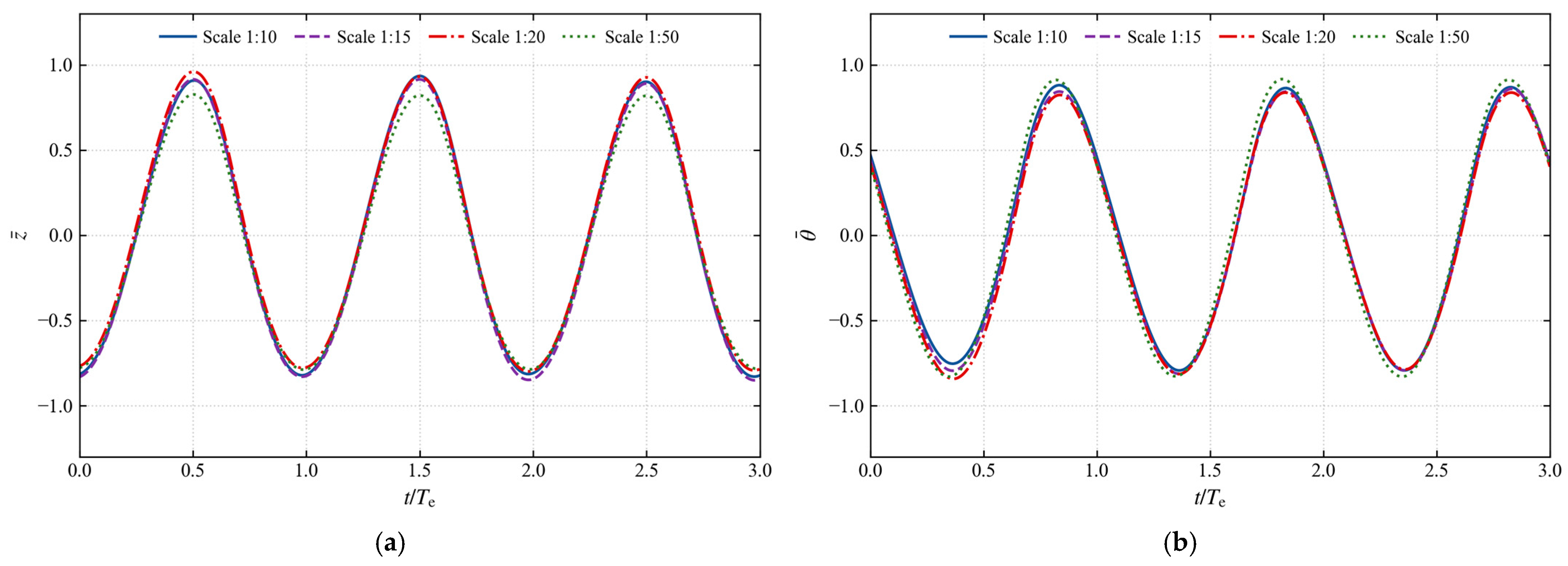
Simulations are performed across four scale ratios (1:10, 1:15, 1:20, and 1:50) under the critical resonant wave condition (λ/L_WL = 1.2). The heave and pitch motions, non-dimensionalized according to Table 3, show good agreement across all four scales (Figure 17). The high overlap of the curves demonstrates that the rigid-body motions are dominated by gravity, buoyancy, and inertia, and thus satisfy Froude similarity across all scales.

As a quantitative verification of Froude similarity,

Table 10. Non-dimensional heave and pitch amplitudes across scale ratios (λ/L_WL = 1.2). Maximum deviation is measured relative to the 1:20 baseline.

Scale Ratio	Heave Amplitude $\overline{\mathit{z}}$	Heave Deviation (%)	Pitch Amplitude $\overline{\mathit{\theta }}$	Pitch Deviation (%)
1:50	0.8038	−8.61%	0.7276	+3.94%
1:20	0.8795	0.00%	0.7000	0.00%
1:15	0.9042	+2.81%	0.7041	+0.59%
1:10	0.8821	+0.30%	0.6992	−0.11%

lists the non-dimensional amplitudes and their deviation from the 1:20 baseline.

The maximum deviation remains within 9% across all scales, confirming that global seakeeping motions satisfy Froude similarity and that the multi-scale simulation set-up is internally consistent. The heave and pitch deviations for the larger models (1:15 and 1:10) are remarkably small, staying well within 3%. The slightly elevated heave deviation (−8.6%) observed at the 1:50 scale is attributed to the relatively coarser absolute free-surface grid spacing and increased numerical damping inherent to extremely small-scale wave propagation.

5.2. Scale Effects on Pressure Coefficient

According to classical Froude scaling law, the slamming pressure scales linearly with the geometric scale ratio α. Mathematically, this relation is derived by assuming that the pressure coefficient C_p is identical across all scale ratios (i.e., C_p,full = C_p,model). The pressure coefficient C_p is defined as:

$$C_{\mathrm{p}}={\displaystyle \frac{P}{\frac{1}{2}\rho U^2}}$$

(12)

Since the density ρ is set constant at 1025.0 kg/m³ across all simulation scales in STAR-CCM+ and the velocity ratio scales as $U_{\mathrm{full}}/U_{\mathrm{model}}=\sqrt{\alpha }$, the Froude similarity pressure scaling law is derived through the following relationship chain:

$$C_{\mathrm{p},\mathrm{full}}=C_{\mathrm{p},\mathrm{model}}\Rightarrow {\displaystyle \frac{P_{\mathrm{full}}}{\frac{1}{2}\rho U_{\mathrm{full}}^2}}={\displaystyle \frac{P_{\mathrm{model}}}{\frac{1}{2}\rho U_{\mathrm{model}}^2}}\Rightarrow P_{\mathrm{full}}=P_{\mathrm{model}}·{\left({\displaystyle \frac{U_{\mathrm{full}}}{U_{\mathrm{model}}}}\right)}^2=P_{\mathrm{model}}·\alpha$$

(13)

In classical ship hydrodynamic testing, slamming pressures are conventionally extrapolated to full scale assuming strict Froude similarity ($C_{\mathrm{p},\mathrm{full}}=C_{\mathrm{p},\mathrm{model}}$), as formulated in Equation (13). However, as highlighted in recent marine hydrodynamic investigations [3,21], this assumption neglects viscous boundary layer development, aeration cushions, and local flow separation at high Reynolds numbers. To capture these viscous scale effects, the multi-scale CFD framework across four geometric scales (1:50, 1:20, 1:15, and 1:10) is evaluated. It is important to emphasize that the regression extrapolation model developed herein serves as an engineering estimation methodology to quantify viscous scaling trends rather than validated experimental benchmark truth.

To eliminate the influence of different incoming wave kinematics across scales, the pressures are non-dimensionalized into the slamming pressure coefficient (C_p).

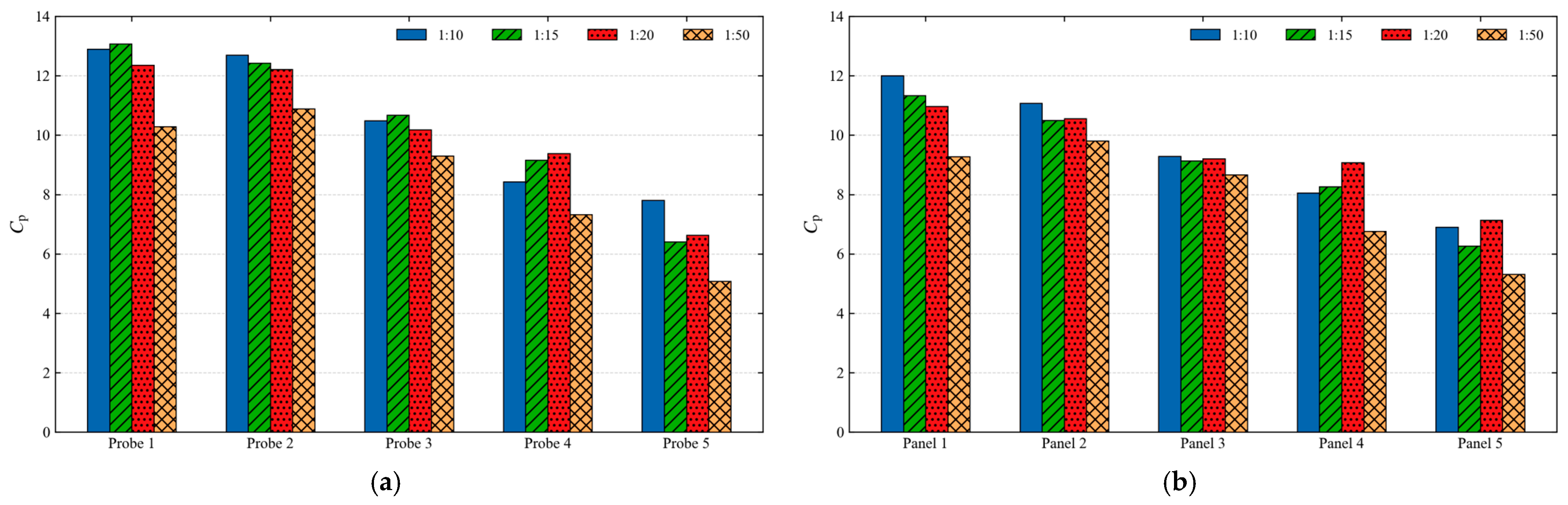
As shown in Figure 18, although the pressure coefficients are in a similar magnitude range across all tested scales, there is a decrease in Cp as the scale ratio α increases (which corresponds to smaller physical sizes). The drop is relatively larger for the 1:50 model. Panel 1 is taken as an example of the most severe impact zone, and its coefficient decreases from 12.00 at the 1:10 scale to 9.28 at the 1:50 scale. Among the larger configurations (1:10, 1:15 and 1:20), the reduction is not strictly monotonic and shows a slight oscillation. Such small data scattering is due to the inherent chaotic and transient nature of fluid impact, as well as wave-by-wave changes when hitting the 3D curvature of the bulbous bow. Although there is some scatter, the overall downward trend significantly violates the assumption of constant C_p in traditional Froude scaling, and other scale effects are taking place.

5.3. Physical Mechanisms of Scale Effects

This observed deviation in C_p at different scales can be related to the Reynolds number (Re) difference in Froude-scaled experiments. Under Froude scaling, the velocity ratio is U_m/U_s = α^−1/2 and the geometric ratio is L_m/L_s = α⁻¹. The model-scale Reynolds number can change according to:

$$R{e}_m={\displaystyle \frac{U_m{L}_m}{\nu }}={\displaystyle \frac{U_s{L}_s}{\nu }}·{\alpha }^{-3/2}=R{e}_s·{\alpha }^{-3/2}\hspace{1em}\hspace{1em}$$

(14)

An increase in the geometric scale ratio α (which means a smaller physical model) leads to a large reduction in the Reynolds number. At a small scale, this low Reynolds number results in a relatively thick boundary layer compared with the hull size. This thicker viscous layer acts as a primary hydrodynamic buffer, dampening the localized slamming jet velocity and reducing the sharp impact pressure peak [2,4]. While the present multi-scale CFD simulations strongly support this viscous boundary layer interpretation, dedicated physical experiments would be valuable in future research to completely isolate viscous damping from other secondary scale-dependent phenomena.

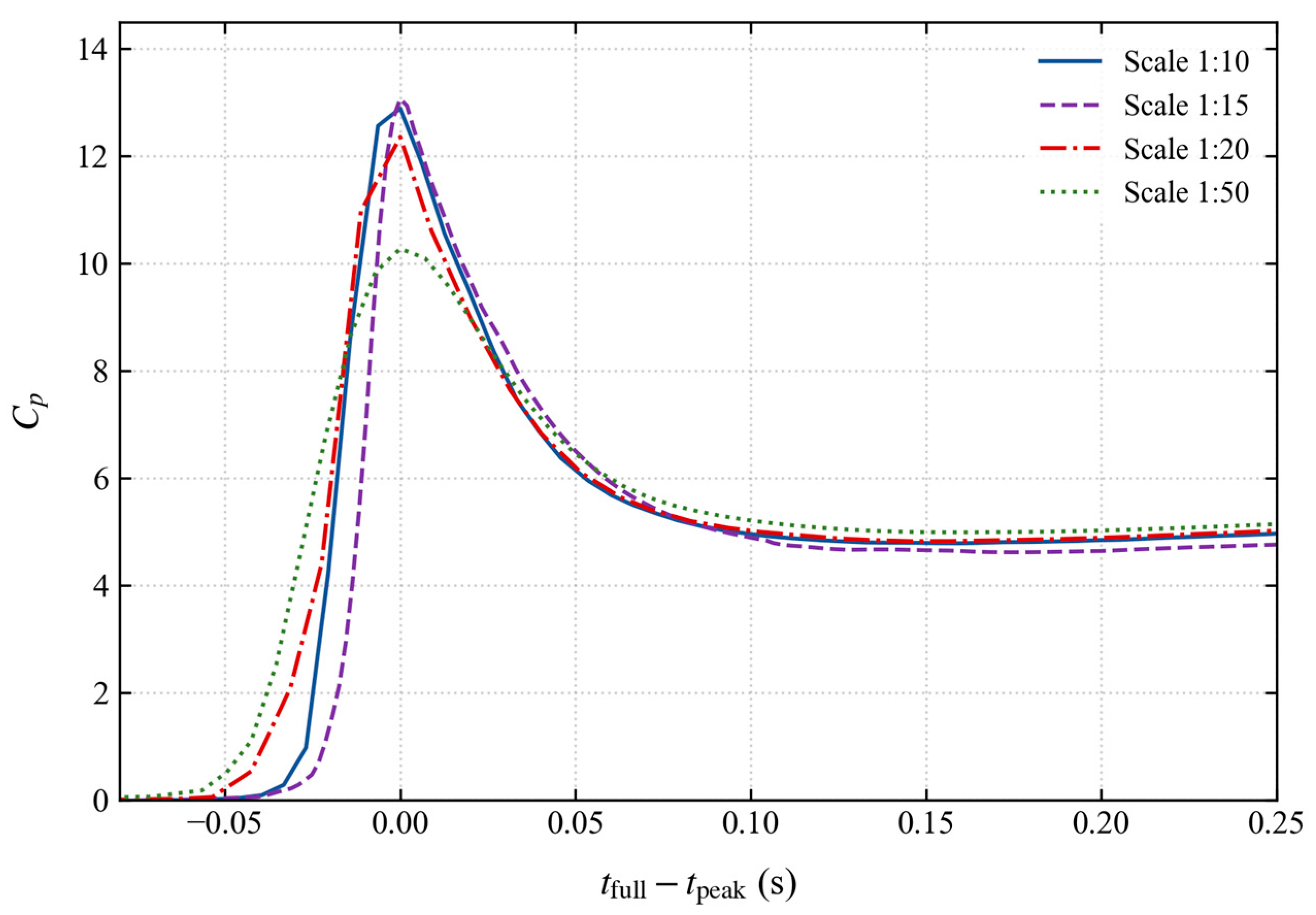
The time-history curves of the pressure also show a similar trend. As shown in Figure 19, the smallest model (1:50 scale) has a lower peak pressure, but its pressure pulse is relatively wide and has a longer rise and decay time compared with those at larger scales. Therefore, the total slamming impulse varies little across different scales. This suggests a self-compensating physical mechanism: viscous scale effects extend the duration of impact and spread out energy over time while maintaining almost the same total momentum transfer [30].

5.4. Multi-Scale Linear Regression Extrapolation

Since the pressure coefficient varies with the scale, it cannot be reliably predicted for the actual full-scale slamming behavior based on the standard Froude number method applied to a single model size. As of now, direct full-scale measurements or simulations for validation are not available, and a multi-scale extrapolation framework will be used to propagate the slamming forces systematically. It has been observed that the Froude-scaled physical pressures (in kPa) are almost linearly related to the scale factor α. Therefore, at each sensor site, a linear regression equation is established to show this change:

$$p_{full}(\alpha )=A\alpha +B$$

(15)

A is the slope of the scale-induced deviation and B is the regression intercept in Equation (15).

Table 11. Model-scale wetted panel peak pressures (in Pa) and the extrapolated full-scale values.

Panel ID	1:50 Scale (Pa)	1:20 Scale (Pa)	1:15 Scale (Pa)	1:10 Scale (Pa)	Full-Scale Extrapolated (kPa)
Panel 1	6739	19,924	27,433	43,635	448.6
Panel 2	7123	19,179	25,426	40,230	403.4
Panel 3	6283	16,718	22,136	33,790	342.7
Panel 4	4904	16,504	20,029	29,273	326.3
Panel 5	3862	12,975	15,197	25,078	264.5

and

Table 12. Model-scale probe local peak pressures (in Pa) and the extrapolated full-scale values.

Probe ID	1:50 Scale (Pa)	1:20 Scale (Pa)	1:15 Scale (Pa)	1:10 Scale (Pa)	Full-Scale Extrapolated (kPa)
Probe 1	7471	22,465	31,670	46,853	499.8
Probe 2	7907	22,176	30,090	46,179	475.2
Probe 3	6753	18,493	25,857	38,149	396.5
Probe 4	5324	17,036	22,181	30,619	344.6
Probe 5	3684	12,045	15,520	28,370	282.5

present the basic model-scale pressure outputs and their Froude-scaled counterparts. According to fluid mechanics theory, the development of a viscous boundary layer is generally proportional to Re^−1/2. Therefore, the base scale effect is inherently non-linear. However, in the specific scale range for analysis here (1:50 to 1:10), a simple linear fit can reproduce the CFD results accurately and consistently reaches an R² value of more than 0.97 in the severe impact area. The above strong correlation shows that linear regression is suitable for engineering estimation of these specific scales; however, extending this linear relationship to a large range of other scales requires further verification.

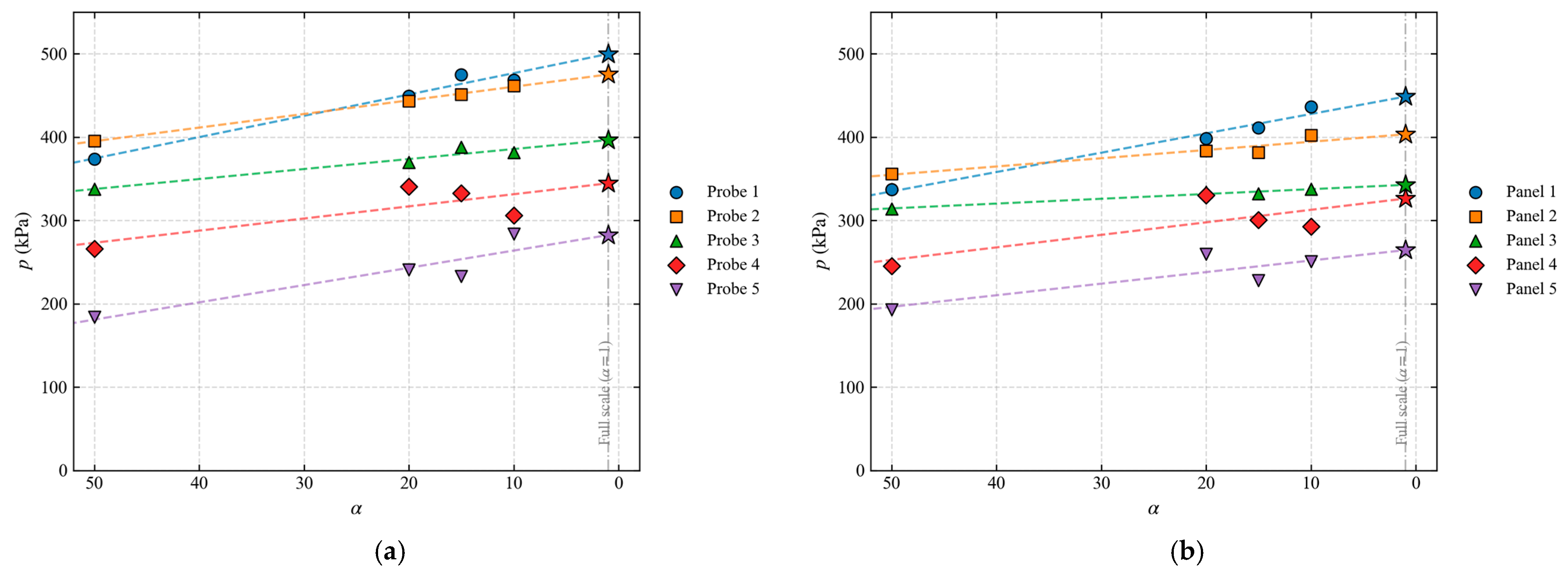
Based on the datasets from Table 11 and Table 12, Figure 20 visually presents the linear regression fits across the four model scales. The regression lines are extended to the full-scale condition, with the extrapolated intercept (α = 1) explicitly highlighted by a star marker.

The exact regression coefficients derived from these fits, including the slope (A), intercept (B), and the coefficient of determination (R²), are quantified in

Table 13. Linear regression coefficients and determination coefficients (R²) for wetted panel and probe pressure extrapolations.

Probe/Panel ID	A	B (kPa)	Se (kPa)	±Δ (%)	R2
Panel 1	−2.3220	450.96	8.6	1.6%	0.9745
Probe 1	−2.5587	502.36	10.3	1.7%	0.9702
Panel 2	−0.9896	404.34	8.4	1.8%	0.8795
Probe 2	−1.6347	476.82	1.3	0.2%	0.9988
Panel 3	−0.5766	343.30	2.7	0.7%	0.9590
Probe 3	−1.1999	397.70	7.3	1.6%	0.9338
Panel 4	−1.5026	327.79	28.8	6.8%	0.5889
Probe 4	−1.4570	346.05	26.9	6.1%	0.6075
Panel 5	−1.3899	265.84	20.4	6.1%	0.7104
Probe 5	−2.0706	284.57	21.4	6.0%	0.8322

.

The regression parameters in Table 13 delineate the physical validity domain of this linear scaling across different bow regions:

(1)

Forward primary impact zone (Panels 1–3, Probes 1–3): The linear fits show excellent correlation, with determination coefficients R² ranging from 0.88 to 0.99 and low standard errors of regression (S_e < 10.3 kPa, relative uncertainty ±Δ < 2.0%). This high linearity confirms that the initial stagnation impact is dominated by self-similar inertia-driven flow, where viscous boundary layer damping scales steadily with Reynolds number.

(2)

Aft keel transition zone (Panels 4–5, Probes 4–5): The regression exhibits moderate dispersion (R² = 0.5889–0.8322, S_e ≈ 20∼29 kPa). This increased scatter is physically caused by progressive 3D flow detachment, lateral spray separation, and turbulent wake disturbances trailing behind the primary impact line [3,30].

(3)

Upper hull panels (Panels 11–25): The structural surfaces experience continuous hydrodynamic wave run-up rather than sharp dynamic slamming shocks. Supplementary verification on the adjacent secondary row (Panels 6–10) confirms similarly robust linearity (R² = 0.93–0.98, such as R² 0.9456 at Probe 7 and 0.9835 at Probe 8), indicating that multi-scale linear regression provides an acceptable engineering estimation within the primary impact region.

Based on this regression, the extrapolated full-scale peak pressure is 448.6 ± 29.2 kPa at Panel 1 and 499.8 ± 38.5 kPa at Probe 1 (within 95% prediction intervals). In contrast, direct Froude scaling from the 1:50 model yields only 336.9 kPa, significantly underestimating the full-scale load by ignoring the reduction in viscous cushioning. Exploring alternative scaling formulations, such as volumetric Reynolds parameters ($Re/\sqrt{\nabla }$) [40] and turbulent boundary-layer models ($\delta /L\propto R{e}^{-1/5}$) [22], represents a promising avenue to refine full-scale load prediction further.

6. Conclusions

An overset-grid RANS-VOF numerical approach was applied to investigate slamming pressures on a 3D bulbous bow in regular head waves across four geometric scale ratios (α = 10, 15, 20, and 50). Based on the multi-scale simulations, the main conclusions are:

(1)

Wave Encounter Condition: The wavelength-to-ship-length ratio λ/L_WL = 1.2 corresponds to the critical slamming condition. At this motion-sensitive condition, the phase relationship between hull motions and incident waves maximizes relative vertical bow velocity, leading to pronounced bow emergence and subsequent water-entry impact.

(2)

Spatial Pressure Distribution: Peak impact pressures concentrate near the forward keel tip of the bulbous bow (Probe 1) and decay steadily along the keel toward the aft section. The 3D convex geometry causes lateral pressure variations around the maximum breadth, while secondary pressure rises occur on upper panels during deeper submergence due to wave run-up.

(3)

Area-Averaging and Impulse Characteristics: Evaluating structural loads solely from localized point probes tends to yield higher localized values than area-integrated measurements. Spatial averaging over a typical structural plate panel (0.6 m × 0.6 m at full scale) results in an effective peak pressure reduction of 11.2–13.5% in the primary impact zone. In addition, the idealized triangular impulse approximation encloses about 72.6–80.6% of the dynamic pressure impulse during the primary shock stage, offering an efficient engineering surrogate for structural dynamic assessments.

(4)

Viscous Scale Effects and Engineering Extrapolation: Extrapolating slamming loads directly from small-scale models using classical Froude scaling tends to underestimate full-scale peak pressures. Numerical analysis indicates that the relatively thicker viscous boundary layer at smaller scales acts as a hydrodynamic cushion, moderating the instantaneous peak pressure while broadening the pulse duration. To characterize this scale-dependent tendency, a multi-scale linear regression framework across four geometric scales (α = 10, 15, 20, 50) was established, exhibiting high linearity (R² = 0.88–0.99, S_e < 10.3 kPa) in the primary impact region. The resulting extrapolated full-scale slamming estimates reach 499.8 ± 38.5 kPa for the localized point probe (Probe 1) and 448.6 ± 29.2 kPa for the area-averaged panel (Panel 1) (representing empirical engineering estimates within 95% prediction intervals). It should be noted that these extrapolated values serve as preliminary engineering references; the linear scaling provides a relatively representative approximation in the primary impact zone, whereas data near the aft keel section exhibit moderate dispersion due to local three-dimensional flow separation and wake dynamics.

In summary, this study highlights the potential limitations of directly applying classical Froude scaling to 3D bulbous bow slamming, and presents a practical multi-scale extrapolation approach. Based on the above research results, engineers can determine a reasonable range of three-dimensional slamming loads for the design of a safe ship in a severe sea state. It should be noted that this study has only used numerical simulations, and direct experimental verification of the bulbous bow pressures has not yet been conducted. Although the numerical framework has passed grid and time-step convergence tests and is consistent with the theoretical wedge water-entry benchmark, the absolute accuracy of the extrapolated full-scale pressures has not yet been confirmed by future physical model tests or full-scale trials. In future work, more experiments, tests with a wider range of scale ratios, and advanced theoretical scaling formulations will be conducted to further refine and validate the extrapolation methodologies.

References

1. Liao, X.; Chen, Z.; Gui, H.; Du, M. CFD Prediction of Ship Seakeeping and Slamming Behaviors of a Trimaran in Oblique Regular Waves. J. Mar. Sci. Eng. 2021, 9, 1151. [Google Scholar] [CrossRef] [Scilit]
2. Kapsenberg, G.K. Slamming of Ships: Where Are We Now? Philos. Trans. R. Soc. A Math. Phys. Eng. Sci. 2011, 369, 2892–2919. [Google Scholar] [CrossRef] [Scilit]
3. Chen, Z.; Jiao, J.; Jiang, C.; Si, H.; Chen, S. Scale Effects on Wave Loads and Slamming Loads in Ship Hydroelasticity Simulation by CFD-FEM Method. Ocean Eng. 2024, 314, 119718. [Google Scholar] [CrossRef] [Scilit]
4. Jiao, J.; Yu, H.; Chen, C.; Ren, H. Time-Domain Numerical and Segmented Model Experimental Study on Ship Hydroelastic Responses and Whipping Loads in Harsh Irregular Seaways. Ocean Eng. 2019, 185, 59–81. [Google Scholar] [CrossRef] [Scilit]
5. Kim, J.-H.; Kim, Y. Numerical Analysis on Springing and Whipping Using Fully-Coupled FSI Models. Ocean Eng. 2014, 91, 28–50. [Google Scholar] [CrossRef] [Scilit]
6. Chang, X.; Chen, Z.; Jiao, J.; Ma, B. Experimental and Numerical Investigation on Springing and Whipping Responses of a 21000TEU Containership. Ocean Eng. 2025, 338, 121979. [Google Scholar] [CrossRef] [Scilit]
7. Wang, Q.; Yu, P.; Zhang, B.; Li, G. Experimental Study and Numerical Simulation of the Water Entry of a Ship-like Symmetry Section with an Obvious Bulbous Bow. Pol. Marit. Res. 2021, 28, 16–34. [Google Scholar] [CrossRef] [Scilit]
8. Wang, S.; Guedes Soares, C. Numerical Study on the Water Impact of 3D Bodies by an Explicit Finite Element Method. Ocean Eng. 2014, 78, 73–88. [Google Scholar] [CrossRef] [Scilit]
9. Wagner, H. Über Stoß- Und Gleitvorgänge an Der Oberfläche von Flüssigkeiten. ZAMM-J. Appl. Math. Mech./Z. Angew. Math. Mech. 1932, 12, 193–215. [Google Scholar] [CrossRef] [Scilit]
10. Korobkin, A.A.; Pukhnachov, V.V. Initial Stage of Water Impact. Annu. Rev. Fluid Mech. 1988, 20, 159–185. [Google Scholar] [CrossRef]
11. Zhao, R.; Faltinsen, O. Water Entry of Two-Dimensional Bodies. J. Fluid Mech. 1993, 246, 593–612. [Google Scholar] [CrossRef] [Scilit]
12. Lin, Y.; Ma, N.; Gu, X. Potential -Flow and CFD Investigations of Bow-Flare Slamming on a Container Ship in Regular Heading Waves. Ocean Eng. 2021, 219, 108278. [Google Scholar] [CrossRef] [Scilit]
13. Wang, Q.; Yu, P.; Chang, X.; Fan, G.; He, G. Research on the Bow-Flared Slamming Load Identification Method of a Large Container Ship. Ocean Eng. 2022, 266, 113142. [Google Scholar] [CrossRef] [Scilit]
14. Jiao, J.; Huang, S.; Tezdogan, T.; Terziev, M.; Guedes Soares, C. Slamming and Green Water Loads on a Ship Sailing in Regular Waves Predicted by a Coupled CFD–FEA Approach. Ocean Eng. 2021, 241, 110107. [Google Scholar] [CrossRef] [Scilit]
15. Acharya, A.; Datta, R. Parametric Study of Bow Slamming for a KRISO Container Ship. Ocean Eng. 2022, 244, 110420. [Google Scholar] [CrossRef] [Scilit]
16. Liu, D.; Li, F.; Liang, X. Numerical Study on Green Water and Slamming Loads of Ship Advancing in Freaking Wave. Ocean Eng. 2022, 261, 111768. [Google Scholar] [CrossRef] [Scilit]
17. Hirt, C.W.; Nichols, B.D. Volume of Fluid (VOF) Method for the Dynamics of Free Boundaries. J. Comput. Phys. 1981, 39, 201–225. [Google Scholar] [CrossRef] [Scilit]
18. Shen, Z.; Wan, D.; Carrica, P.M. Dynamic Overset Grids in OpenFOAM with Application to KCS Self-Propulsion and Maneuvering. Ocean Eng. 2015, 108, 287–306. [Google Scholar] [CrossRef] [Scilit]
19. Jiao, J.; Chen, C.; Ren, H. A Comprehensive Study on Ship Motion and Load Responses in Short-Crested Irregular Waves. Int. J. Nav. Archit. Ocean Eng. 2019, 11, 364–379. [Google Scholar] [CrossRef] [Scilit]
20. Ping, Y.; Wang, J.; Xie, H.; Liu, F.; Liu, X. Experimental and CFD Analysis: Effects of Bottom Appendages on the Slamming Characteristics of Rigid Hull Structures during Water Entry. Ocean Eng. 2025, 319, 120195. [Google Scholar] [CrossRef] [Scilit]
21. Huang, L.; Pena, B.; Thomas, G. Towards a Full-Scale CFD Guideline for Simulating a Ship Advancing in Open Water. Ship Technol. Res. 2023, 70, 222–238. [Google Scholar] [CrossRef] [Scilit]
22. Jiao, J.; Huang, S. CFD Simulation of Ship Seakeeping Performance and Slamming Loads in Bi-Directional Cross Wave. J. Mar. Sci. Eng. 2020, 8, 312. [Google Scholar] [CrossRef] [Scilit]
23. Huo, F.; Wei, C.; Zhu, C.; Yuan, Z.; Xu, S. Research on the Water Ridge and Slamming Characteristics of a Semisubmersible Platform under Towing Conditions. J. Mar. Sci. Eng. 2022, 10, 116. [Google Scholar] [CrossRef] [Scilit]
24. Chen, Z.; Jiao, J.; Wang, Q.; Wang, S. CFD-FEM Simulation of Slamming Loads on Wedge Structure with Stiffeners Considering Hydroelasticity Effects. J. Mar. Sci. Eng. 2022, 10, 1591. [Google Scholar] [CrossRef] [Scilit]
25. Li, Z.; Zan, Y.; Guo, R.; Sun, Y.; Sun, N. Dynamic Characteristics and Flow Field Evolution of Flat Plate Water Entry Slamming Based on Smoothed Particle Hydrodynamics. J. Mar. Sci. Eng. 2024, 12, 1491. [Google Scholar] [CrossRef] [Scilit]
26. Wang, W.; Piao, T.; Geng, C.; Zhang, K.; Wang, Z.; Huang, Y. Slamming Characteristics Due to the Special Shape of New Sandglass-Type Model in Waves by Comparing with Cylindrical Model. J. Mar. Sci. Eng. 2024, 12, 712. [Google Scholar] [CrossRef] [Scilit]
27. Kim, Y.J.; Kim, K.-H.; Nam, B.W.; Hong, S.Y.; Ha, Y.-J. Numerical Study of Slamming Loads on Bow Flare of FPSO Model by Irregular Waves. J. Mar. Sci. Eng. 2025, 13, 455. [Google Scholar] [CrossRef] [Scilit]
28. Maki, K.J.; Lee, D.; Troesch, A.W.; Vlahopoulos, N. Hydroelastic Impact of a Wedge-Shaped Body. Ocean Eng. 2011, 38, 621–629. [Google Scholar] [CrossRef] [Scilit]
29. Krasilnikov, V.; Skjefstad, V.S.; Koushan, K.; Rambech, H.J. A Calibration Study with CFD Methodology for Self-Propulsion Simulations at Ship Scale. J. Mar. Sci. Eng. 2023, 11, 1342. [Google Scholar] [CrossRef] [Scilit]
30. Abrahamsen, B.C.; Grytten, F.; Andreassen, E.; Hellan, Ø. Hydroelastic Response of Froude Scaled Stiffened Steel Panels Exposed to Design-Critical Wave Slamming. Appl. Ocean Res. 2023, 141, 103774. [Google Scholar] [CrossRef] [Scilit]
31. Hosseinzadeh, S.; Tabri, K. Hydroelastic Effects of Slamming Impact Loads during Free-Fall Water Entry. Ships Offshore Struct. 2021, 16, 68–84. [Google Scholar] [CrossRef] [Scilit]
32. Antolik, J.T.; Belden, J.L.; Speirs, N.B.; Harris, D.M. Slamming Forces during Water Entry of a Simple Harmonic Oscillator. J. Fluid Mech. 2023, 974, A23. [Google Scholar] [CrossRef] [Scilit]
33. Panciroli, R.; Shams, A.; Porfiri, M. Experiments on the Water Entry of Curved Wedges: High Speed Imaging and Particle Image Velocimetry. Ocean Eng. 2015, 94, 213–222. [Google Scholar] [CrossRef] [Scilit]
34. Huo, F.; Yang, H.; Yao, Z.; An, K.; Xu, S. Study on Slamming Pressure Characteristics of Platform under Freak Wave. J. Mar. Sci. Eng. 2021, 9, 1266. [Google Scholar] [CrossRef] [Scilit]
35. Shih, T.-H.; Liou, W.W.; Shabbir, A.; Yang, Z.; Zhu, J. A New k-ϵ Eddy Viscosity Model for High Reynolds Number Turbulent Flows. Comput. Fluids 1995, 24, 227–238. [Google Scholar] [CrossRef] [Scilit]
36. Wang, Z.; Li, T.; Ren, J.; Jin, Q.; Zhou, W. URANS Calculation of Ship Heave and Pitch Motions in Marine Simulator Based on Overset Mesh. J. Mar. Sci. Eng. 2022, 10, 1374. [Google Scholar] [CrossRef] [Scilit]
37. Zhang, X.; Lin, Z.; Mancini, S.; Li, P.; Liu, D.; Liu, F.; Pang, Z. Numerical Investigation into the Effect of Damage Openings on Ship Hydrodynamics by the Overset Mesh Technique. J. Mar. Sci. Eng. 2020, 8, 11. [Google Scholar] [CrossRef] [Scilit]
38. Tezdogan, T.; Demirel, Y.K.; Kellett, P.; Khorasanchi, M.; Incecik, A.; Turan, O. Full-Scale Unsteady RANS CFD Simulations of Ship Behaviour and Performance in Head Seas Due to Slow Steaming. Ocean Eng. 2015, 97, 186–206. [Google Scholar] [CrossRef] [Scilit]
39. Korobkin, A.A. A Linearized Model of Water Exit. J. Fluid Mech. 2013, 737, 368–386. [Google Scholar] [CrossRef] [Scilit]
40. Beji, S. Formulation of Wave and Current Forces Acting on a Body and Resistance of Ships. Ocean Eng. 2020, 218, 108121. [Google Scholar] [CrossRef] [Scilit]
Figure 1. Schematic illustration of the ship hull geometry, coordinate system, and bulbous bow division: (a) Schematic 3D view of the generic hull form and coordinate system; (b) Subdivided pressure panels (labels in red) and localized pressure monitoring points (labels in blue) on the bulbous bow.
Jmse 14 01593 g001
Figure 2. Numerical computational domain size and boundary conditions.
Jmse 14 01593 g002
Figure 3. Overset grid layout and local refinement zones: (a) Overall computational domain mesh and multi-level refinement blocks; (b) Overset boundary interface and background mesh transition; (c) Overset mesh block surrounding the hull; (d) Bulbous bow surface mesh and prism boundary layers.
Jmse 14 01593 g003
Figure 4. Wall y+ distribution on the hull and bulbous bow surface for the 1:20 baseline model.
Jmse 14 01593 g004
Figure 5. Numerical wave tank verification and calibration: (a) Free-surface wave elevation contour; (b) Spatial wave profile comparison with Stokes 5th-order theory; (c) Wave elevation time histories at three probes.
Jmse 14 01593 g005
Figure 6. Computed volume fraction contour (free-surface profile) during the 2D wedge water entry.
Jmse 14 01593 g006
Figure 7. Numerical verification and benchmarking of 2D wedge water entry: comparison of pressure coefficient Cp along the wedge surface with similarity and BEM solutions of Zhao and Faltinsen [11].
Jmse 14 01593 g007
Figure 8. Mesh configurations for grid refinement comparison: (a) Coarse mesh configuration (2.07 M cells); (b) Medium mesh configuration (3.43 M cells); (c) Fine mesh configuration (4.38 M cells).
Jmse 14 01593 g008
Figure 9. Grid convergence study of ship motion responses: (a) Non-dimensional heave motion; (b) Non-dimensional pitch motion.
Jmse 14 01593 g009
Figure 10. Grid convergence study of local slamming pressure at Probe 1.
Jmse 14 01593 g010
Figure 11. Convergence study of global motions and local slamming pressure at Probe 1 under different time steps: (a) Non-dimensional heave motion; (b) Non-dimensional pitch motion; (c) Local slamming pressure coefficient.
Jmse 14 01593 g011
Figure 12. Non-dimensional motion response time histories (heave and pitch) under three different wavelength ratios: (a) Non-dimensional heave motion; (b) Non-dimensional pitch motion.
Jmse 14 01593 g012
Figure 13. High-resolution sequence of 3D free surface deformation during bow slamming impact: (a) t = 19.60 s; (b) t = 19.64 s; (c) t = 19.68 s; (d) t = 19.72 s; (e) t = 19.76 s; (f) t = 19.80 s.
Jmse 14 01593 g013
Figure 14. Time history of pressure coefficient (Cp) at keel centerline over three encounter cycles under critical wave condition (λ/LWL = 1.2): (a) Panel-averaged pressures; (b) Localized probe pressures.
Jmse 14 01593 g014
Figure 15. Longitudinal keel centerline monitoring points (BottomP1 to BottomP12): (a) Spatial layout on ship bottom (colored patches indicate individual subdivided structural panels); (b) Peak slamming pressure distributions across scale ratios.
Jmse 14 01593 g015
Figure 16. Comparison between instantaneous CFD slamming pressure time histories and the idealized triangular impulse model: (a) Probe 1; (b) Probe 2; (c) Probe 3.
Jmse 14 01593 g016
Figure 17. Non-dimensional motion responses across four scale ratios: (a) Heave motion; (b) Pitch motion.
Jmse 14 01593 g017
Figure 18. Slamming pressure coefficient (Cp) at five monitoring locations across four scale ratios. (a) Localized point probes. (b) Area-averaged panels.
Jmse 14 01593 g018
Figure 19. Pressure time histories at Probe 1 normalized to the full-scale time frame, illustrating the broader pulse shape at smaller scales.
Jmse 14 01593 g019
Figure 20. Linear regression of Froude-scaled slamming pressures versus scale ratio α, extrapolated to full scale (α = 1, where colored star markers denote the extrapolated full-scale values): (a) Localized point probes. (b) Area-averaged panels.
Jmse 14 01593 g020