Article

A Statistical Quality-Control Framework for Sentinel-1 SAR Wind Speed Retrieval Based on First- and Second-Order Moments

1
College of Marine Sciences, Fujian Agriculture and Forestry University, Fuzhou 350002, China
2
College of Ocean and Earth Sciences, Xiamen University, Xiamen 361102, China
3
Dongshan Swire Marine Station, Xiamen University, Xiamen 361005, China
4
State Key Laboratory of Satellite Ocean Environment Dynamics, Second Institute of Oceanography, Ministry of Natural Resources, Hangzhou 310012, China
5
College of Physics and Electronic Information Engineering, Minjiang University, Fuzhou 350108, China
6
Fuzhou Institute of Oceanography, Minjiang University, Fuzhou 350108, China
*
Authors to whom correspondence should be addressed.
J. Mar. Sci. Eng. 2026, 14(16), 1555; https://doi.org/10.3390/jmse14161555
Submission received: 22 July 2026 / Revised: 18 August 2026 / Accepted: 20 August 2026 / Published: 21 August 2026
(This article belongs to the Section Physical Oceanography)

Abstract

Synthetic Aperture Radar (SAR) enables high-resolution sea-surface wind speed retrieval. However, the enhanced spatial resolution of SAR imagery introduces substantial challenges, from small-scale contamination sources that significantly degrade retrieval accuracy. Particularly in coastal regions, non-wind-related backscatter signals, such as ships and oil slicks, can severely bias wind speed estimates at sub-kilometer scales. In this study, the first-order moment (average, m1) and second-order moment (variance, m2) are computed from the normalized radar cross-section (NRCS) within sub-images of Sentinel-1 SAR data acquired in Interferometric Wide (IW) mode. Analysis reveals that clean-sea-surface signals in both VV and VH polarizations cluster around an approximately linear empirical trend, m2 = 2m1 + b, in the m1-m2 statistical feature space, whereas the examined contamination types deviate from this trend and occupy separable regions. Based on this characteristic, a quality-control framework is proposed for the systematic separation of clean sea surface from image noise (border noise and inter-swath stripe noise) and non-ocean targets (land contamination, bright targets, and dark spots). Validation using independent SAR data from the Taiwan Strait was conducted separately for native 10 m and height-adjusted 3 m buoy observations. For the native 10 m observations, the RMSE and MBE were essentially unchanged at 1.5 m/s and −0.3 m/s, respectively. For the height-adjusted nearshore observations, the RMSE decreased from 3.2 m/s to 2.1 m/s and the MBE changed from −1.5 m/s to −1.1 m/s.

1. Introduction

Synthetic Aperture Radar (SAR) provides high-resolution observations of the ocean surface under nearly all weather conditions and independently of solar illumination [1,2]. Unlike an in situ anemometer, however, SAR does not measure the wind directly. Instead, it records the normalized radar cross-section (NRCS, denoted as σ0), which represents the electromagnetic response of the sea-surface at the sensor wavelength and acquisition geometry. Wind modifies the short gravity-capillary waves responsible for Bragg-scale scattering, but the observed NRCS is also modulated by wave development and swell, surface currents, atmospheric stability, sea surface temperature, surface films, precipitation, incidence angle, relative azimuth, and polarization. The relationship between NRCS and the local wind vector is therefore nonlinear and not necessarily unique, particularly in heterogeneous coastal waters and under dynamically complex ocean conditions [3,4,5,6,7,8,9,10].
Recovering the 10 m equivalent neutral wind from SAR NRCS is consequently an inverse problem. Geophysical Model Functions (GMFs), such as CMOD5.N for C-band VV-polarized observations, describe NRCS as a nonlinear function of wind speed, incidence angle, and the angle between the wind direction and the radar look direction [11]. Their inversion therefore requires accurate acquisition geometry and wind-direction information. Moreover, similar SAR intensities may arise from different combinations of wind forcing, sea state, currents, surface films, rain, and other geophysical processes. SAR intensity alone is therefore insufficient to uniquely determine a complete wind-vector field or to distinguish all wind-induced roughness variations from non-wind-related backscatter signatures. Recent spatial and data-driven retrieval approaches similarly emphasize the need to combine nonlinear NRCS–wind mappings with contextual or spatial information [12].
Variational methods can reduce inversion ambiguity by combining SAR observations with background wind information and spatial constraints [13,14]. However, because the solution remains dependent on the background field, model assumptions, and input NRCS quality, these methods cannot independently recover all fine-scale turbulent variability from SAR intensity alone. This limitation highlights the need to identify contaminated backscatter measurements before wind retrieval.
Current sensors such as Sentinel-1 can achieve spatial resolutions of 10 m or better, enabling the capture of fine-scale wind field structures essential for understanding mesoscale atmospheric phenomena and supporting disaster early warning systems. However, this enhanced resolution simultaneously amplifies the impact of small-scale contamination sources on retrieval accuracy. In coastal waters, where anthropogenic activities result in dense concentrations of vessels, aquaculture facilities, offshore platforms, and other artificial structures, this challenge becomes particularly acute. These targets, though occupying only a few pixels in SAR imagery, produce radar returns that deviate substantially from wind-dependent sea-surface backscatters, thereby introducing systematic biases into retrieved wind fields at sub-kilometer scales. Xu et al. documented that ship traffic and ocean fronts near estuarine regions lead to systematic overestimation of SAR-derived winds [15], while Jang et al. investigated additional influences from bathymetry, sand ridge, and radar interference in coastal environments [16]. Beyond anthropogenic targets, oil slicks dampen sea-surface roughness and manifest as dark spots in SAR imagery, and image artifacts such as border noise and inter-swath stripe noise may introduce additional localized errors. When such contaminated pixels are included in wind retrieval processing, they degrade the reliability of the retrieved wind fields.
The objective of this study is to develop a statistical quality-control (QC) framework for Sentinel-1 IW mode SAR wind speed retrieval using the first-order moment (average, m1) and second-order moment (variance, m2) of sub-image NRCS. The methodological contribution is threefold: (1) to characterize the approximately linear empirical trend of clean-sea-surface sub-images in the m1-m2 statistical feature space for both VV and VH polarizations; (2) to formulate polarization-dependent classification windows for screening the examined border noise, inter-swath stripe noise, land contamination, bright targets, and dark spots within a unified framework; and (3) to evaluate the transferability and practical effect of the framework using an independent Sentinel-1 dataset from the Taiwan Strait and collocated buoy observations. The framework is intended as a pre-retrieval QC procedure: it improves the reliability of the NRCS inputs to CMOD5.N-based wind speed retrieval but does not independently retrieve wind direction or reconstruct complete spatial wind vectors.

2. Data and Processing

2.1. Data

2.1.1. Sentinel-1 SAR Imagery

This study utilizes Sentinel-1 Ground Range Detected (GRD) SAR imagery acquired in Interferometric Wide (IW) swath mode. This mode employs the Terrain Observation by Progressive Scans SAR (TOPSAR) technique, enabling wide-area coverage while maintaining relatively high spatial resolution. The SAR imagery with IW mode utilized in this study provides three sub-swaths with incidence angles ranging from 29.1° to 46.0° and a spatial resolution of 10 m × 10 m.
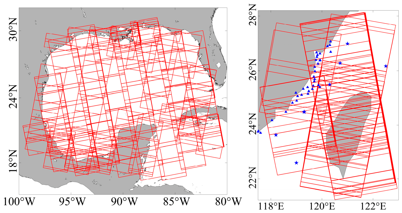
For the establishment of the QC framework, SAR images over the Gulf of Mexico are collected, comprising 4193 VV-polarized and 3775 VH-polarized images acquired between 2016 and 2019. For validation, the SAR images from waters surrounding Taiwan Island are collected, comprising 2055 VV-polarized images acquired between 2014 and 2024. The coverage area of these SAR images is shown in Figure 1.

2.1.2. Buoy Winds

Wind speed measurements from 42 moored buoys during January 2021 to March 2023 are employed to evaluate the SAR-derived wind speeds. The wind speeds are measured at heights of 3 m (number: 35) and 10 m (number: 7) above sea level and recorded every 10 min. The positions of these buoys are shown in Figure 1. For validation purposes, the 3 m wind measurements are converted to 10 m equivalent neutral winds using the logarithmic wind profile [17]:
U 10 = U z k v 2 C d 1 ln ( z / z 0 )
where kv is the von Kármán constant (approximately 0.4), Cd is the drag coefficient (1.2 × 10⁻³), z0 is the roughness length (9.7 × 10⁻⁵), and U10 (Uz) represents wind speed at the height of 10 m (z m).

2.1.3. CCMP and ERA5 Reanalysis Winds

In this study, the Cross-Calibrated Multi-Platform (CCMP) wind fields were utilized as background fields to assist in retrieving winds from SAR images. When CCMP data were unavailable, the European Centre for Medium-Range Weather Forecasts (ECMWF) reanalysis v5 (ERA5) data served as a supplement to maintain the continuity of the background fields. CCMP is a synthesized product of ERA5 winds and winds retrieved from multiple satellite microwave sensors. The CCMP data have a spatial and temporal resolution of 0.25° and 6 h, respectively [18], while ERA5 data have the same spatial resolution of 0.25° but with a finer temporal resolution of 1 h [19].

2.1.4. GSHHG Coastline Data

The Global Self-consistent, Hierarchical, High-resolution Geography (GSHHG) coastline database was employed in this study for the land masking of SAR imagery [20]. Due to the dynamic nature of coastlines, some land pixels in SAR imagery may remain after masking, which are subsequently detected as coastal land residuals in the QC framework.

2.2. Sub-Image Statistics Computation

For subsequent analysis, each SAR image was segmented into non-overlapping sub-images, each comprising 50 × 50 pixels (500 m × 500 m). For each sub-image, the first-order moment and second-order moment were computed as follows:
m 1 L = 1 n i = 1 n σ 0 , i
m 2 L = 1 n i = 1 n ( σ 0 , i m 1 L ) 2
m 1 = 10 × log 10 ( m 1 L )
m 2 = 10 × log 10 ( m 2 L )
where n denotes the number of pixels within the sub-image, and σ 0 , i represents the NRCS value (in linear units) at the i-th pixel. Superscript L indicates values in linear units, while m1 and m2 without superscripts denote the corresponding values in decibel (dB) units. All Sentinel-1 IW images used here have a pixel spacing of 10 m, and the 50 × 50-pixel window defines a common statistical scale of 500 m × 500 m; m2 therefore describes NRCS variability within this window rather than wind speed variance itself. It should be emphasized that m1 and m2 are descriptive statistics of the observed NRCS and do not separate the processes that generate the observed variability. Tidal currents, short-term wind fluctuations, incidence-angle variation across the 29.1–46.0° range, polarization, and the fixed segmentation of coastal scenes all contribute to the distributions analyzed below, and their effects remain embedded in m1 and m2 rather than being modeled explicitly. The classification thresholds derived in Section 3 are consequently empirical and apply to the polarization, sub-image scale, and preprocessing configuration specified here.

3. Analysis

3.1. Border Noise

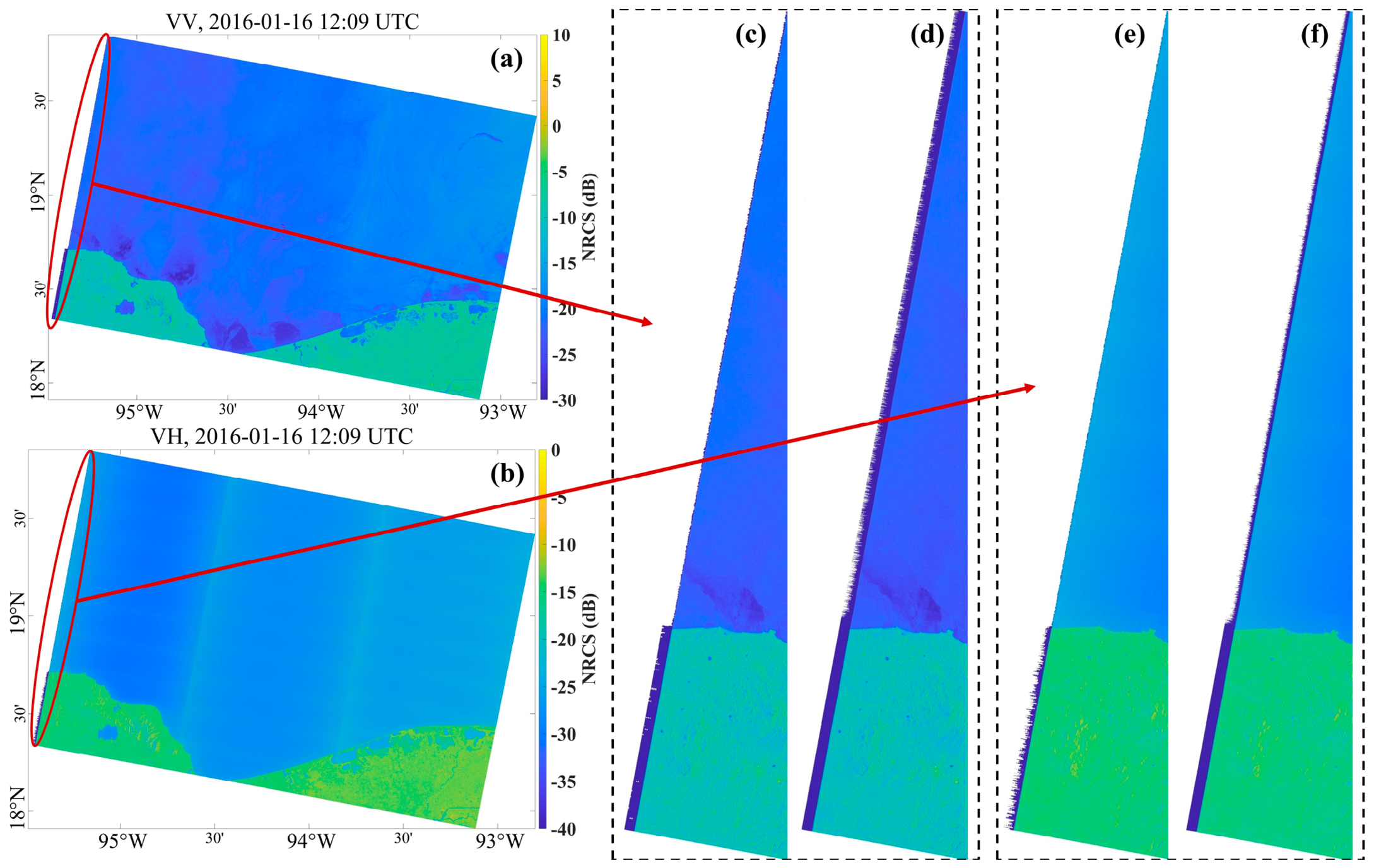
Border noise arises during the generation of Level-1 products from Level-0 data through azimuth and range compression processing, combined with Sampling Window Start Time (SWST) handling [21]. Figure 2 illustrates the border noise in Sentinel-1 SAR imagery. Figure 2a,b presents co-located VV-polarized and VH-polarized images acquired over the Gulf of Mexico at 12:09 UTC on 16 January 2016. The red-circled regions highlight the border areas, which are enlarged in Figure 2c–f for detailed examination. Figure 2c and Figure 2e display the original SAR images for VV and VH polarizations, respectively, while Figure 2d,f show the corresponding images after 5-look multi-look processing. The multi-look process effectively reduces speckle noise but enhances the visibility of systematic border noise patterns along the image edges. As evident in the enlarged views, the border regions exhibit anomalous backscatter values. If left uncorrected, this artifact may affect image mosaic and introduce bias in quantitative analyses such as wind speed retrieval or oil slick detection.
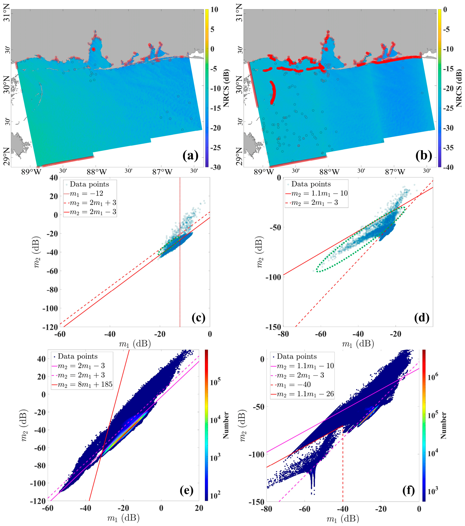
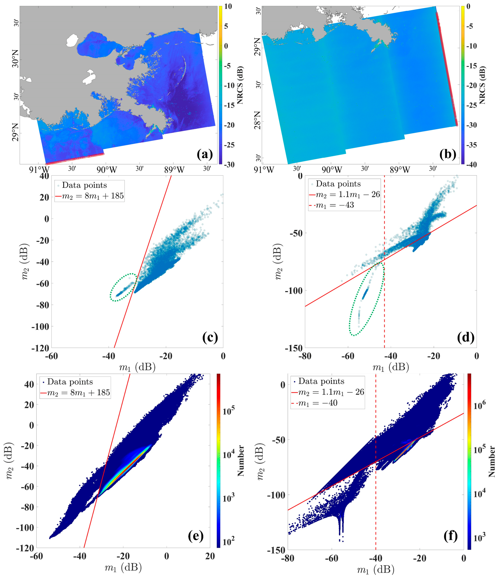
Figure 3 demonstrates border-noise detection based on the m1-m2 space. Figure 3a presents the VV-polarized SAR image acquired at 00:02 UTC on 15 May 2016, and Figure 3b presents the VH-polarized image acquired at 00:01 UTC on 28 January 2016. The corresponding m1-m2 scatter plots for these individual images are shown in Figure 3c and Figure 3d, respectively, where the straight lines delineate the classification boundaries. For the VV-polarized image, border noise is detected by m 2 8 m 1 + 185 ; for the VH-polarized image, border noise is detected by m 1 43   dB and m 2 1.1 m 1 26 . Data points corresponding to the detected border noise are indicated by green dashed ellipses in Figure 3c,d, with the corresponding pixels marked by small red circles in Figure 3a,b.
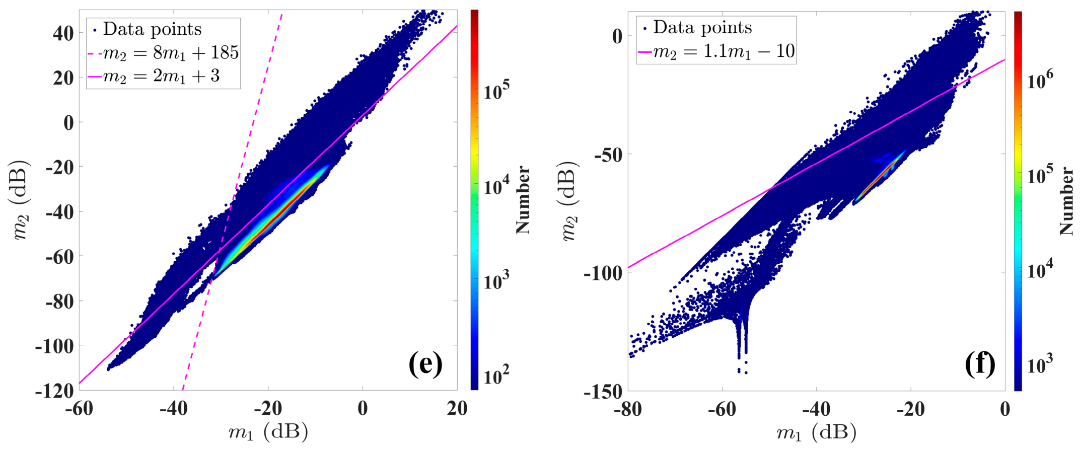
Figure 3e,f extends this analysis to the entire Gulf of Mexico dataset, encompassing all VV-polarized and VH-polarized images. The aggregated distributions confirm that the m1-m2 linear relationship is consistent across the dataset. To facilitate operational implementation, the batch processing formulas are derived from the aggregated distributions:
For VV polarization, the batch processing formula is:
m 2 8 m 1 + 185
for VH polarization, the batch processing formula is:
m 1 40   dB   and   m 2 1.1 m 1 26
It should be noted that there is an inherent trade-off between individual image processing and batch processing approaches. The batch processing formulas in (6) and (7) represent generalized thresholds optimized for the entire dataset, which may not capture atypical border-noise patterns present in individual images.

3.2. Inter-Swath Stripe Noise

Inter-swath stripe noise, commonly referred to as the banding effect, results from residual noise after noise equivalent sigma zero (NESZ) correction [22]. This occurs because: (1) NESZ does not accurately describe the noise floor across all conditions [23]; and (2) sub-swath boundaries exhibit higher scattering entropy due to multiplicative noise that NESZ correction cannot fully remove [24].
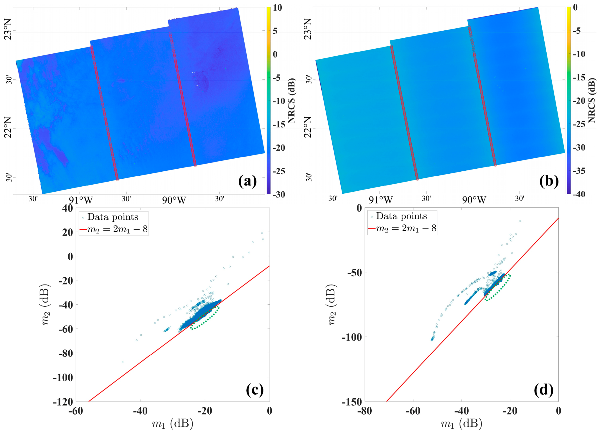
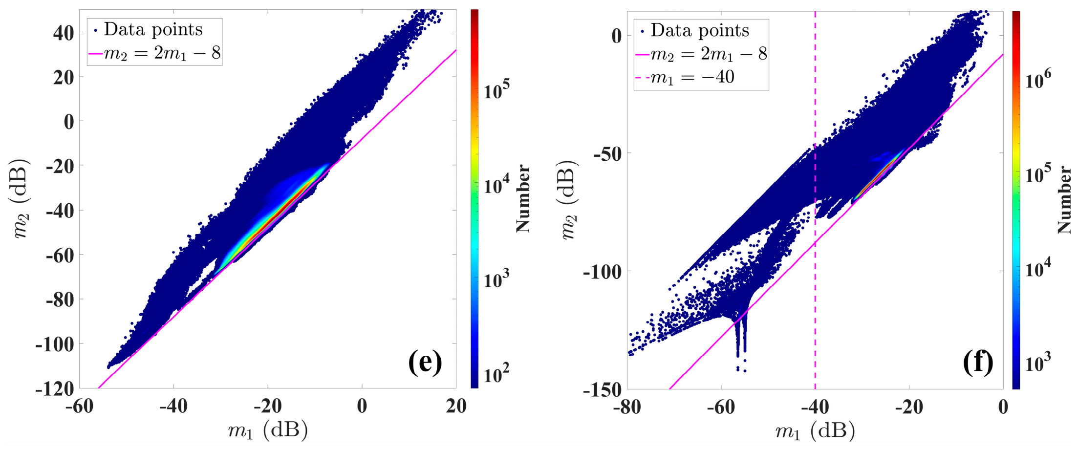
Figure 4 illustrates the detection of inter-swath stripe noise in IW mode SAR imagery. Figure 4a,b presents VV-polarized and VH-polarized SAR images acquired at 00:07 UTC on 27 January 2017. The corresponding m1-m2 scatter plots for these individual images are shown in Figure 4c and Figure 4d, respectively. Data points corresponding to the detected noise are indicated by green dashed ellipses in Figure 4c,d, with the corresponding pixels marked by small red circles in Figure 4a,b. Figure 4e,f extends this analysis to the entire Gulf of Mexico dataset.
For VV polarization, the batch processing formula is:
m 2 2 m 1 8
For VH polarization, the batch processing formula is same as (8), but with an additional constraint of m 1 > 40   dB .
In both polarization channels, the distribution of the inter-swath stripe noise in the m1-m2 space is highly stable across different images, consistently appearing below the straight line m 2 =   2 m 1 8 .

3.3. Land Contamination

Despite land masking using GSHHG coastline data, some high-σ0 land pixels may remain in the processed imagery due to dynamic coastline changes from natural processes (sea level rise, storms, tides) and human activities (coastal construction, land reclamation). These residual signals significantly affect wind retrieval accuracy in nearshore regions.
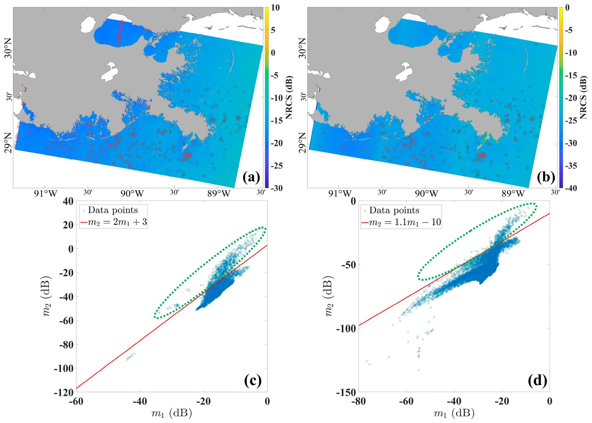
Figure 5 presents the detection of coastal land residuals in IW mode SAR imagery. Figure 5a,b displays VV-polarized and VH-polarized SAR images acquired at 23:53 UTC on 22 January 2016. The corresponding m1-m2 scatter plots for these individual images are shown in Figure 5c and Figure 5d, respectively. For the VV-polarized image, coastal land residuals are detected by m 1 12   dB and 2 m 1 3 m 2 2 m 1 + 3 ; for the VH-polarized image, the residuals are detected by 2 m 1 3 m 2 1.1 m 1 10 . Data points corresponding to the detected residuals are indicated by green dashed ellipses in Figure 5c,d, with the corresponding pixels marked by small red circles in Figure 5a,b. Figure 5e,f extends this analysis to the entire Gulf of Mexico dataset.
For VV polarization, the batch processing formula is:
m 2 < 8 m 1 + 185   and   2 m 1 3 m 2 2 m 1 + 3
For VH polarization:
2 m 1 3 m 2 1.1 m 1 10
Notably, VH polarization provides superior capability of detecting land contamination due to the enhanced backscatter contrast between land and ocean.

3.4. Bright Targets

Bright targets encompass vessels, buoys, offshore platforms, and other anthropogenic targets that produce significantly higher radar returns than surrounding sea surfaces due to strong specular reflection and corner reflector effects. In high-resolution SAR imagery, even small vessels occupying just a few pixels can bias local wind estimates.
Figure 6 illustrates the detection of bright targets in IW mode SAR imagery. Figure 6a,b displays VV-polarized and VH-polarized SAR images acquired at 12:06 UTC on 16 January 2016. The corresponding m1-m2 scatter plots for these individual images are shown in Figure 6c and Figure 6d, respectively. For the VV-polarized image, the bright targets are detected by m 2 2 m 1 + 3 ; for the VH-polarized image, the bright targets are detected by m 2 1.1 m 1 10 . Data points corresponding to the detected bright targets are indicated by green dashed ellipses in Figure 6c,d, with the corresponding pixels marked by small red circles in Figure 6a,b. Figure 6e,f extends this analysis to the entire Gulf of Mexico dataset. The aggregated distributions confirm that bright targets consistently occupy the upper region of the m1-m2 space. For VV polarization:
2 m 1 + 3 m 2 < 8 m 1 + 185
For VH polarization:
m 2 > 1.1 m 1 10
While both bright targets and coastal land residuals appear above the main cluster and occupy comparable regions in the m1-m2 space, the former exhibit systematically higher m2 values.

3.5. Dark Spots

Cox and Munk [25] established the fundamental relationship between wind speed and mean square slope for both clean and slick sea surface. Building upon this foundation, the m1-m2 space can be employed to distinguish clean sea surface from dark-spots in SAR imagery. Since VH polarization exhibits reduced sensitivity to wind-induced surface roughness compared to VV polarization, dark spot analysis in this study focuses on VV polarization.
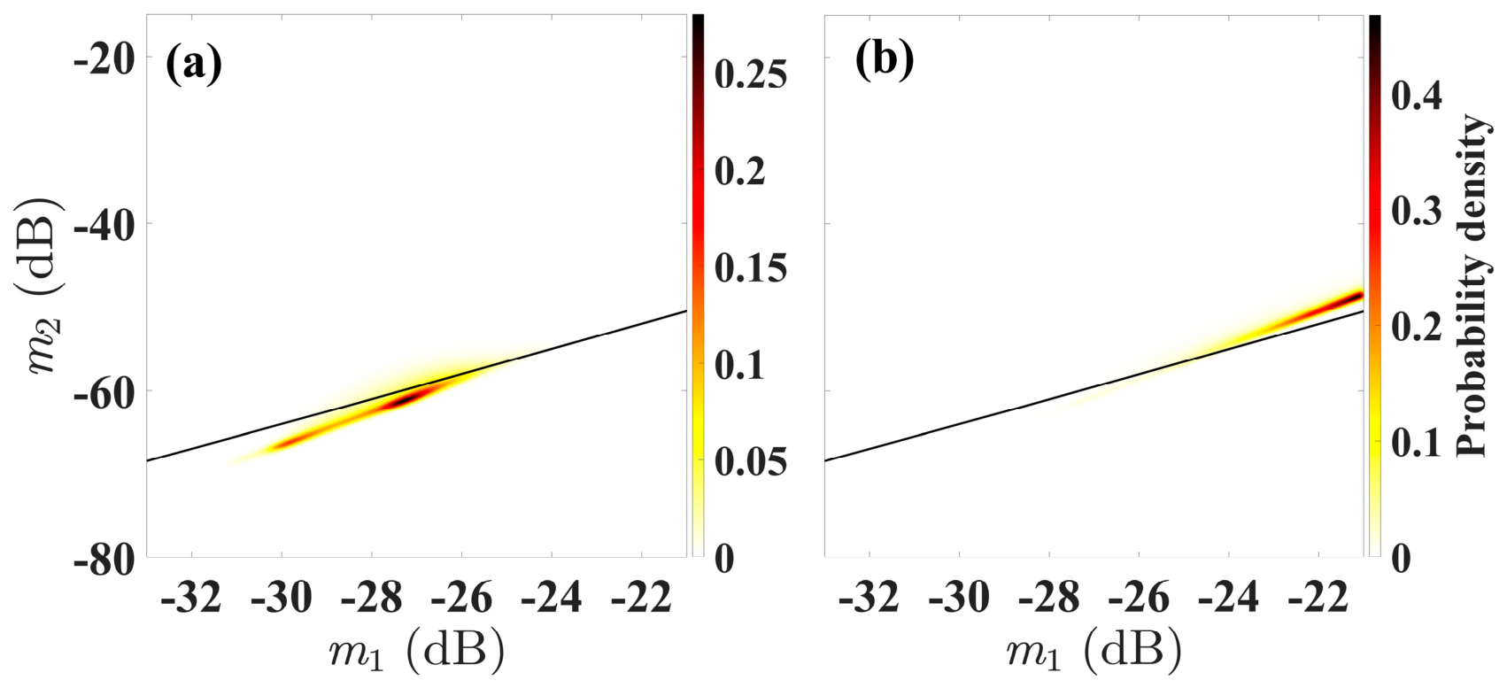
Dark spots correspond to low-σ0 regions caused by a variety of marine phenomena, including oil spills, biogenic films, low wind speed zones, internal waves, sea ice, upwelling areas, and rain cells [26,27]. Using kernel density estimation to compare probability density distributions of slick and clean surface samples, we derived:
m 2 1.5 m 1 19
The detailed derivation process can be found in Appendix A.
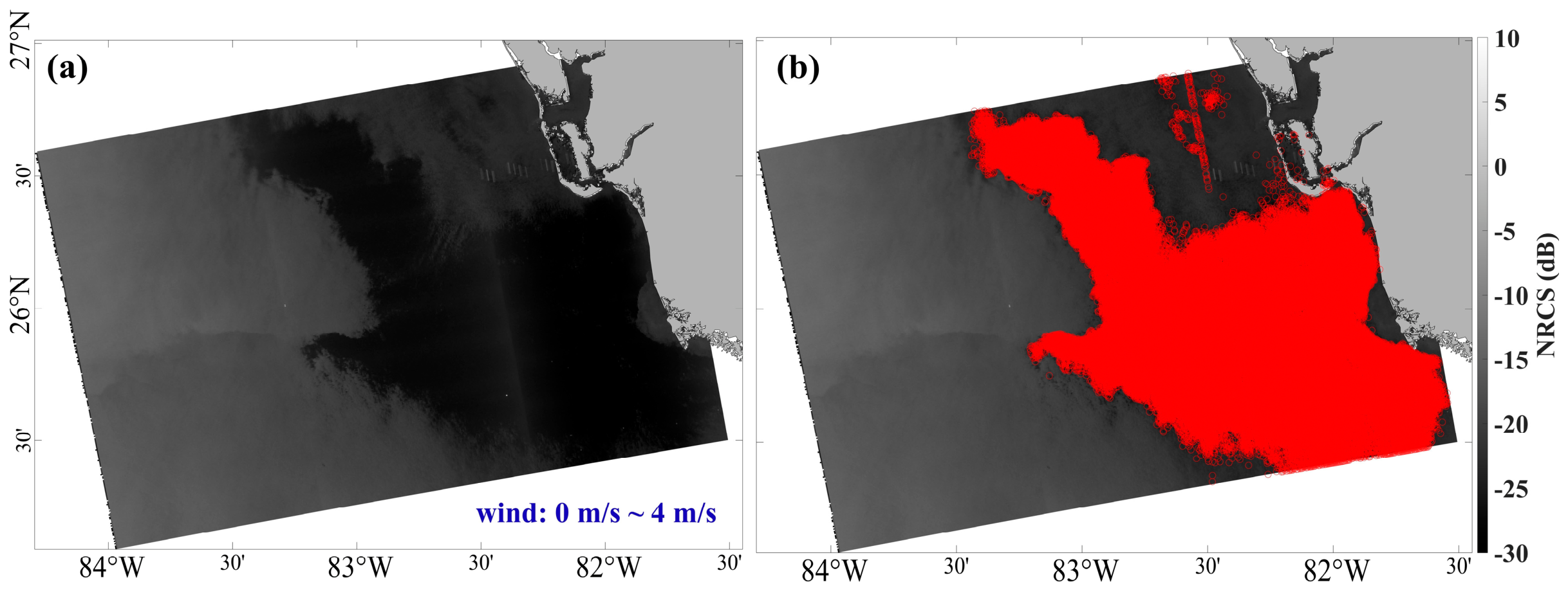
Figure 7 demonstrates the detection of dark spots in VV-polarized SAR imagery. Figure 7a presents a VV-polarized SAR image acquired at 23:36 UTC on 30 April 2017, with wind speeds ranging from 0 to 4 m/s. Figure 7b displays the corresponding detection result, where pixels satisfying (13) are identified as dark spots and highlighted in red.

3.6. The m1-m2 Windows for Clean Sea Surface

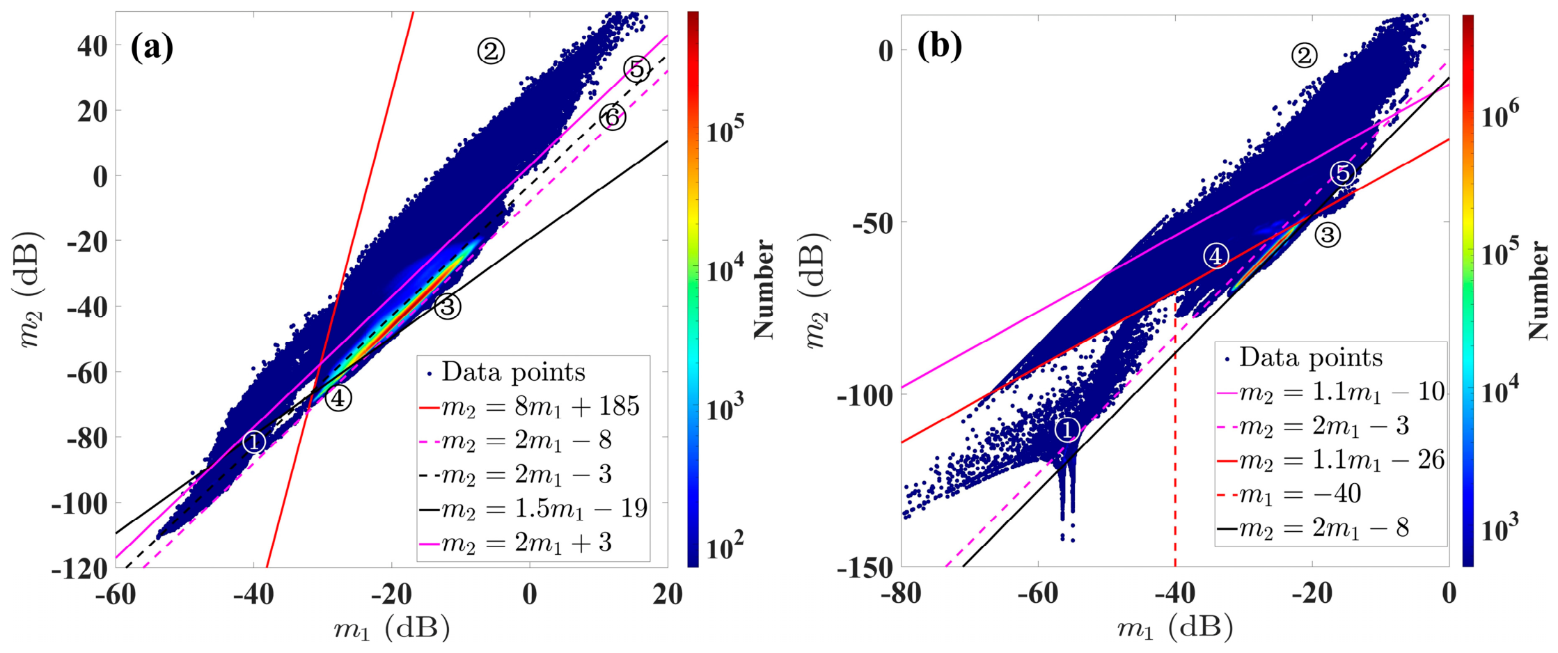
Figure 8 presents a summary of the QC framework based on the m1-m2 space for Sentinel-1 IW mode SAR imagery. The classification boundaries derived from the preceding analyses are superimposed, partitioning the feature space into distinct regions corresponding to different backscatter signal categories.
As summarized in Table 1, for VV polarization, the m1-m2 space is divided into six regions. Region ① ( m 2 8 m 1 + 185 ) corresponds to border noise. Region ② ( 2 m 1 + 3 m 2 < 8 m 1 + 185 ) corresponds to bright targets. Region ③ ( m 2 2 m 1 8 ) corresponds to inter-swath stripe noise. Region ④ ( m 2 < 8 m 1 + 185 and m 2 1.5 m 1 19 ) corresponds to dark spots. Region ⑤ ( m 2 < 8 m 1 + 185 and 2 m 1 3 m 2 < 2 m 1 + 3 ) corresponds to land contamination and other features (such as partial border noise). The remaining region, Region ⑥, corresponds to clean sea surface.
For VH polarization, the m1-m2 space is divided into five regions. Region ① ( m 1 40   d B and m 2 1.1 m 1 26 ) corresponds to border noise, Region ② ( m 2 > 1.1 m 1 10 ) corresponds to bright targets, Region ③ ( m 1 > 40   d B and m 2 2 m 1 8 ) corresponds to inter-swath stripe noise. Region ④ ( 2 m 1 3 m 2 1.1 m 1 10 ) corresponds to land contamination. The remaining region, Region ⑤, corresponds to clean sea surface. Notably, the VH classification framework does not include a separate dark-spot category, as VH-polarized backscatter is less sensitive to the Bragg-scale wave damping that characterizes oil slicks, making dark-spot detection primarily reliant on VV polarization.
Consequently, the extraction of clean sea surface from VV-polarized imagery satisfies the following conditions:
m 2 < 8 m 1 + 185
m 2 > 1.5 m 1 19
2 m 1 8 < m 2 < 2 m 1 3
For the extraction of clean sea surface from VH-polarized imagery, condition (16) applies, along with:
m 1 > 40   dB
It can be observed that clean-sea-surface pixels in both VV and VH polarizations satisfy (16). Converting the variables in this expression from logarithmic (dB) to linear units yields:
10 0.8 < m 2 L m 1 L 2 < 10 0.3
where m 2 L m 1 L 2 is the normalized variance.
Equations (2)–(18) serve sequential but distinct roles in the QC and validation workflow. Specifically, Equations (2)–(5) calculate the first- and second-order NRCS moments and construct the m1-m2 statistical feature space. Equations (6)–(13) define contamination-specific classification criteria, whereas Equations (14)–(17) combine these criteria to identify clean-sea-surface sub-images. Equation (18) expresses the common clean surface condition in terms of normalized variance.

4. Results and Discussion

4.1. Wind Retrieval Optimization

To evaluate the effectiveness of the proposed QC framework, Equations (14)–(16) were applied to the dataset comprising 2055 VV-polarized SAR images acquired over the Taiwan Strait.
In this study, either CCMP or ERA5 wind fields served as background fields for input into the CMOD5.N. Employing a variational method [13,14], the sea surface wind speeds were retrieved from these SAR images. The formula of CMOD5.N is presented as:
σ 0 s i m = B 0 ( U 10 , θ ) B 1 ( U 10 , θ ) c o s ( φ ) + B 2 ( U 10 , θ ) c o s ( 2 φ ) 1.6
where σ 0 s i m is the simulated NRCS in linear units, θ is the incidence angle, and φ is the angle between wind direction and SAR azimuth look angle. Coefficients B0, B1, and B2 are empirically derived functions of wind speed and incidence angle. The procedure of retrieving wind fields from SAR images is divided into the following steps.
Step 1: SAR preprocessing. Sentinel-1 VV-polarized data were preprocessed to obtain the calibrated NRCS and the corresponding incidence-angle information.
Step 2: Wind-cell construction. The SAR image was divided into wind cells (i.e., sub-SAR images with 50 × 50 pixels) at the prescribed retrieval resolution. Each wind cell represents one wind speed retrieval unit.
Step 3: Calculation of cell-scale statistical and geometric inputs. For each wind cell, the m1 and m2 of the VV-polarized NRCS were calculated according to Equations (2)–(5). Here, m1 represents the mean NRCS within the wind cell and is used as the observed NRCS input for wind retrieval, whereas m2, expressed as the variance, characterizes the within-cell NRCS variability. The local incidence angle was interpolated to the corresponding wind-cell position.
Step 4: Preparation of the background wind field. The CCMP or ERA5 background wind field was spatially and temporally interpolated to the center of each wind cell. The resulting background wind speed and direction were used as constraints for resolving the directional ambiguity of the SAR observations.
Step 5: For each wind cell, candidate wind speeds from 0 to 35 m/s in steps of 1 m/s and candidate wind directions from 0° to 359° in steps of 1° were generated. For each candidate, the wind direction relative to the radar look direction was calculated, as required by CMOD5.N.
Step 6: Quality-control screening. The m1 and m2 values of each wind cell were evaluated using the polarization-specific criteria defined in the proposed QC framework. Wind cells identified as border noise, inter-swath stripe noise, coastal land contamination, bright targets, or dark spots were excluded from the subsequent retrieval. Only wind cells classified as clean sea surface were retained.
Step 7: CMOD5.N forward calculation and variational optimization. For each QC-retained wind cell, candidate wind components u and v were used to calculate the corresponding wind speed and relative wind direction. CMOD5.N was then applied to simulate the VV-polarized NRCS, σ 0 s i m . The cost function was defined as:
J = u u b Δ u 2 + v v b Δ v 2 + m 1 10 × l g σ 0 s i m Δ σ 2
where ub and vb are the eastward and northward components of background field, respectively. In addition, Δ u = 2 m/s, Δ v = 2 m/s, Δ σ = 0.1 dB. The candidate pair that minimized J was selected as the optimal wind vector. The optimal SAR-derived wind speed was subsequently calculated.
Step 8: Wind speed reconstruction. The optimal wind speeds retrieved for all valid wind cells were assembled according to their geographic positions to produce the final SAR-derived sea-surface wind speed. Wind cells rejected by the QC procedure were marked as invalid and were not assigned retrieved wind values.
Due to the SAR-derived winds having a spatial resolution of 500 m and the buoy winds being reported every 10 min, a matchup dataset is generated by the following criteria: for temporal matching, buoy observations are selected within 10 min before or after the satellite overpass time; for spatial matching, the collocated wind cells closest to the buoys are selected, with the cell-buoy distance shorter than 500 m.
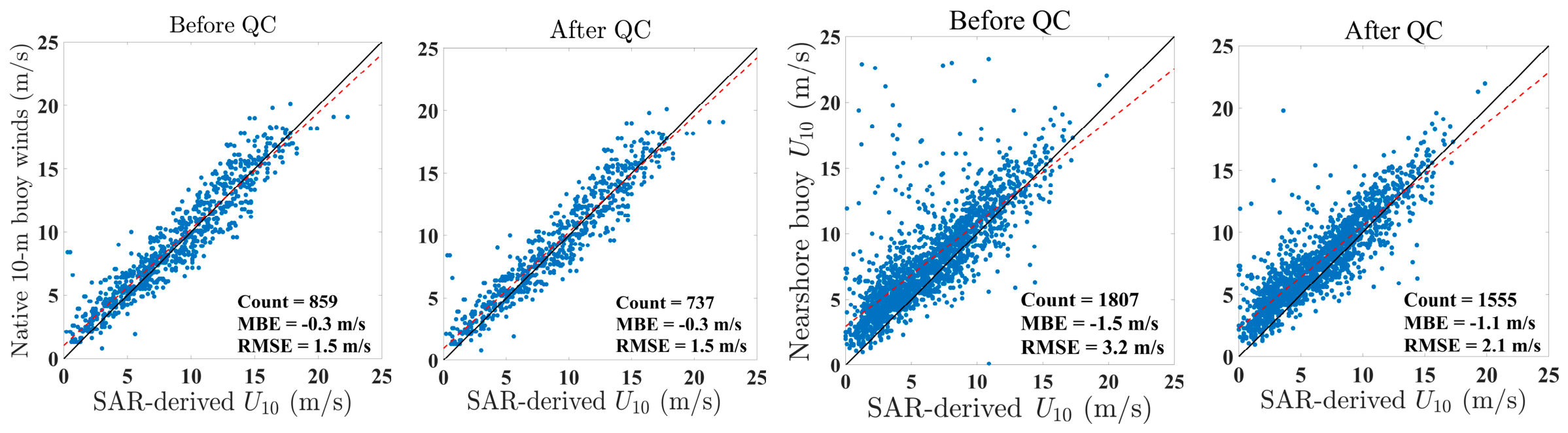
To avoid the uncertainty introduced by converting 3 m wind measurements to a height of 10 m, the SAR-derived wind speeds were first evaluated against the seven buoys measuring wind directly at 10 m, which were located predominantly in offshore waters. Before QC, 859 collocations yielded a root mean square error (RMSE) of 1.5 m/s and a mean bias error (MBE) of −0.3 m/s (the first panel of Figure 9). QC flagged 122 of these collocations (14.2%), and the 737 retained pairs gave essentially the same statistics, 1.5 m/s and −0.3 m/s (the second panel of Figure 9).
The buoys measuring wind at 3 m were concentrated in nearshore waters, where land residuals, vessels, coastal infrastructure, and dark surface features occur more frequently. For this subset, QC flagged a comparable fraction of the collocations (252 of 1807, 13.9%), yet the RMSE decreased from 3.2 m/s to 2.1 m/s and the MBE changed from −1.5 m/s to −1.1 m/s. The contrast between the two subsets therefore lies not in how many cells are rejected but in how strongly the rejected cells were biased. Offshore, removing 122 cells left the error statistics unchanged, indicating that their retrieved speeds already agreed with the buoy values as closely as those of the retained population. Nearshore, the rejected cells were dominated by land contamination (227 of 252), which produced the largest single-filter improvement in Table 2. Because the nearshore observations were converted to 10 m equivalent neutral winds, they are reported separately and should be interpreted with consideration of the uncertainty associated with the height adjustment.
To quantify the contribution of each contamination filter, each filter was applied independently to the same 1807 nearshore SAR-buoy collocations (Table 2). Without QC, the validation yielded an MBE of −1.5 m/s and an RMSE of 3.2 m/s. The border-noise, inter-swath-stripe-noise, and dark-spot filters produced little change in RMSE, consistent with the small numbers of affected collocations. Applying the bright-target filter reduced the RMSE to 2.9 m/s, while the MBE remained −1.5 m/s. The land-contamination filter produced the largest individual improvement, reducing the RMSE to 2.6 m/s and the magnitude of the MBE to 1.2 m/s. The full QC framework retained 1555 collocations and achieved an RMSE of 2.1 m/s and an MBE of −1.1 m/s. This represents a 34.4% reduction in RMSE relative to the no-QC condition. These results indicate that land contamination was the dominant error source in this nearshore subset, while the remaining filters provided additional improvement. This result is consistent with the spatial concentration of land residuals, coastal infrastructure, and other non-ocean targets around the nearshore buoy stations.

4.2. Preliminary Analysis of EW Mode

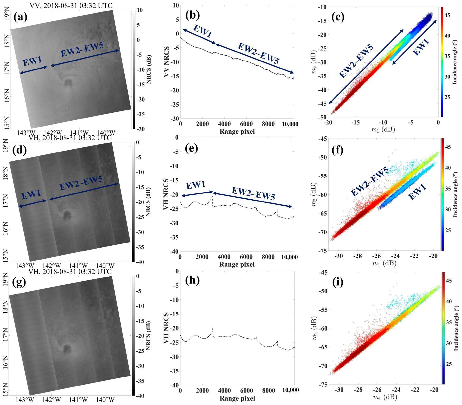
While this study focuses primarily on IW mode imagery, the proposed framework can be extended to Extra Wide (EW) mode. Preliminary analysis of EW mode data reveals a notable discrepancy between the first sub-swath (EW1) and the remaining sub-swaths (EW2–EW5) in VH polarization.
Figure 10 illustrates this issue using the SAR image with EW mode acquired at 03:32 UTC on 31 August 2018. Figure 10a–c shows the original VV-polarized image, the corresponding σ0 variation along the range direction, and the m1-m2 distribution, respectively. The VV channel exhibits a smooth and continuous σ0 transition across the swath. Figure 10d–f present the original VH-polarized image. Unlike VV polarization, the VH-polarized σ0 profile in Figure 10e reveals noticeable discontinuities at sub-swath boundaries, particularly between EW1 and EW2. This inconsistency is evident in the m1-m2 space shown in Figure 10f, where a distinct cluster corresponding to EW1 appears offset from the main cluster by approximately 1 dB.
Since the incidence-angle range of EW2–EW5 is largely consistent with that of IW mode, we attribute the observed ~1 dB offset to characteristics specific to EW1. To harmonize the five sub-swaths, a correction was applied by subtracting 1 dB from VH-polarized σ0 values within EW1. As shown in Figure 10g–i, the previously separated EW1 cluster has merged with the main cluster, resulting in a more homogeneous image. Consequently, for applications such as tropical cyclone wind retrieval, EW mode data require correction for the systematic σ0 offset between EW1 and the remaining sub-swaths. The correction method proposed herein may serve as a viable approach.

5. Conclusions

This study developed a comprehensive QC framework for high-resolution SAR wind speed retrieval based on the m1-m2 relationship. Here, m1 denotes the first-order statistical moment, i.e., the mean NRCS within each 50 × 50-pixel sub-image, whereas m2 denotes the second-order statistical moment, i.e., the NRCS variance. Their linear-unit values are converted to decibels for the m1-m2 analysis. The main findings are summarized as follows:
(1)
In both VV- and VH-polarized imagery, the m1 and m2 of clean-sea-surface sub-images cluster around an approximately linear empirical trend, m2 = 2m1 + b, with the intercept b typically between −8 and −3 dB. This trend provides the baseline against which contaminated sub-images are identified.
(2)
Different backscatter signal types occupy separable regions in the m1-m2 space: border noise appears in low-m1 regions; inter-swath stripe noise appears below the main cluster; land contamination and bright targets appear above the cluster; and dark spots in VV-polarized imagery satisfy m 2 1.5 m 1 19 .
(3)
Height-stratified validation showed that, for native 10 m buoy observations, the RMSE and MBE remained at 1.5 m/s and −0.3 m/s, respectively, after quality control (QC), with 737 of 859 collocations retained. For nearshore observations measured at 3 m and converted to 10 m equivalent neutral winds, QC reduced the RMSE from 3.2 m/s to 2.1 m/s and changed the MBE from −1.5 m/s to −1.1 m/s.
A further limitation follows from the design of the dark-spot criterion. Damping-type dark signatures and genuine low-wind areas share almost the same low-backscatter, low-contrast appearance in single-channel SAR intensity, and the present criterion does not separate them; genuine low-wind cells are therefore removed together with slick-like signatures. The practical cost is limited, because the CMOD5.N inversion is ill-conditioned below roughly 2 m/s and retrievals in this range are unreliable irrespective of QC. Uncertainty in this study is quantified at the level of the retrieval statistics rather than at the level of the classification. The MBE and RMSE reported for each QC configuration in Table 2 are accompanied by 95% confidence intervals, which show that the improvement obtained with the full framework exceeds the sampling uncertainty of the nearshore collocation set. No corresponding uncertainty is attached to the class assignments themselves, because the classification thresholds are deterministic and were derived empirically from the aggregated Gulf of Mexico distributions rather than from a probabilistic classifier. Furthermore, because labeled reference data are not available for all five contamination types, conventional detection metrics such as precision and recall cannot be computed, and the sensitivity of the retained sample size and of the retrieval statistics to perturbations of the threshold values has likewise not been quantified. The filter-wise ablation in Table 2 provides only indirect evidence in this respect: it identifies land contamination and bright targets as the filters that control the retrieval improvement and therefore indicates that threshold perturbations in the remaining three filters would have limited practical effect on the present dataset. A labeled validation set and a systematic threshold-perturbation analysis are both needed before the thresholds are applied beyond the configuration examined in this study.
The present framework focuses on statistical quality control followed by CMOD5.N-based wind speed retrieval and independent buoy validation. Radiometrically calibrated Sentinel-1 NRCS is averaged within sub-images at the retrieval scale, and contamination that alters the sub-image mean or variance is evaluated in the m1-m2 feature space. Spatial texture, gradients, and anisotropy may influence these statistical moments; however, the moments do not explicitly retain the spatial arrangement of the NRCS values. Future studies could therefore combine the present statistical screening with spatial–morphological descriptors and two-dimensional spatial spectral analysis, followed by separately validated classification of coherent, frontal, wave-related, turbulent, and contaminated signatures. These developments would extend the method from image quality control toward ocean-feature interpretation and are not prerequisites for the the wind speed QC examined here. Although application to the independent Taiwan Strait dataset provides preliminary evidence of cross-regional applicability, it does not demonstrate that the empirical thresholds are universally transferable. The distributions of m1 and m2 may vary with polarization, incidence angle, sub-image scale, preprocessing settings, regional sea state, and seasonal conditions. Therefore, the present thresholds should be further evaluated and, if necessary, recalibrated before application to other sensors, acquisition modes, spatial resolutions, or ocean regions. Future work will assess their robustness using multi-regional and multi-seasonal Sentinel-1 datasets.

Author Contributions

Conceptualization, Y.W., Y.L. and X.G.; methodology, Y.W.; validation, Y.W. and X.L.; formal analysis, X.L. and C.L.; investigation, Y.W. and C.L.; data curation, F.Z.; writing—original draft preparation, Y.W.; writing—review and editing, S.S.; visualization, Y.W.; supervision, X.G.; project administration, C.L.; funding acquisition, C.L. and S.S. All authors have read and agreed to the published version of the manuscript.

Funding

This research was supported in part by the Major Science and Technology Project of Fuzhou (No. 2024-ZD-018, funded by Fuzhou Science and Technology Bureau), the Fujian Province Natural Science Foundation (Nos.2023J011573 and 2023J011570, funded by Fujian Provincial Department of Science and Technology), and the “Top Talents Recruitment” Science and Technology Project (No. 2025F03, funded by Fuzhou Marine Research Institute).

Data Availability Statement

The original contributions presented in this study are included in the article. Further inquiries can be directed to the corresponding authors.

Acknowledgments

The authors would like to thank the European Space Agency for providing the Sentinel-1 data (https://dataspace.copernicus.eu/ (accessed on 3 May 2025)), the Copernicus for providing the ERA5 data (https://cds.climate.copernicus.eu/ (accessed on 10 June 2025)), Remote Sensing Systems for providing the CCMP data (https://www.remss.com/measurements/ccmp/ (accessed on 10 June 2025)), the NOAA for providing the GSHHG data (https://www.ngdc.noaa.gov/mgg/shorelines/shorelines.html (accessed on 26 October 2024)), and Fujian Marine Forecasts for providing the buoy data (https://www.fjhyyb.cn/ (accessed on 24 May 2023)).

Conflicts of Interest

The authors declare no conflicts of interest.

Appendix A

Cox and Munk conducted extensive airborne experiments to investigate the statistical characteristics of sun glitter patterns on the sea surface [25]. Through systematic analysis, they derived an empirical relationship between the mean square slope of the sea surface (s2) and wind speed under varying wind-direction conditions:
s 2 = ( 5.12 U 12.5 + 3 ) × 10 3 r = 0.986   for   clean   surface ( 1.56 U 12.5 + 8 ) × 10 3 r = 0.770   for   slick   surface  
where U12.5 is the wind speed (m/s) at a height of 12.5 m (41 feet) above the sea surface, and r is the correlation coefficient.
To standardize wind speed measurements, the wind speed at an arbitrary height z is converted to the 10 m height (U10) using Equation (1). Applying this conversion, the relationship between U10 and s2 becomes:
s 2 = ( 5.22 U 10 + 3 ) × 10 3   for   clean   surface ( 1.59 U 10 + 8 ) × 10 3   for   slick   surface  
It is well known that the NRCS (i.e., σ0) in SAR imagery is governed by sea-surface roughness. Given that dark spots typically exhibit relatively low backscatter intensities, the Small Perturbation Method (SPM) [28] provides an appropriate framework for interpreting the electromagnetic scattering mechanism. Under the SPM formulation, the VV-polarized NRCS is expressed as:
σ 0 = 8 k 4 δ 2 cos 4 θ α VV 2 W
where k represents the wave number, δ represents the root mean square of the sea-surface height, θ is the incidence angle, α VV is a polarization-dependent coefficient determined by incidence angle and the complex permittivity of seawater, and W is the roughness spectrum of the sea surface.
The relationship between δ2 and s2 is given by:
s 2 = 2 δ 2 l 2
where l represents the correlation length of the sea surface. Combining Equations (A3) and (A4) yields:
σ 0 s 2 = C
where C is a proportionality constant. Integrating Equations (A2) and (A5), the relationship between σ0 at any pixel in the SAR image and the corresponding wind speed (U10) can be expressed as:
σ 0 = C s 2 = C ( 5.22 U 10 + 3 )   × 10 3   for   clean   surface ( 1.59 U 10 + 8 )   × 10 3   for   slick   surface  
Considering the inherent speckle noise in SAR imagery, the spatially averaged σ0 within each sub-image (i.e., m 1 L ) is utilized. Accordingly, Equation (A6) becomes:
m 1 L = C s 2 = C ( 5.22 U ¯ 10 + 3 )   × 10 3   for   clean   surface ( 1.59 U ¯ 10 + 8 )   × 10 3   for   slick   surface  
where U ¯ 10 represents the mean wind speed within the SAR sub-image footprint.
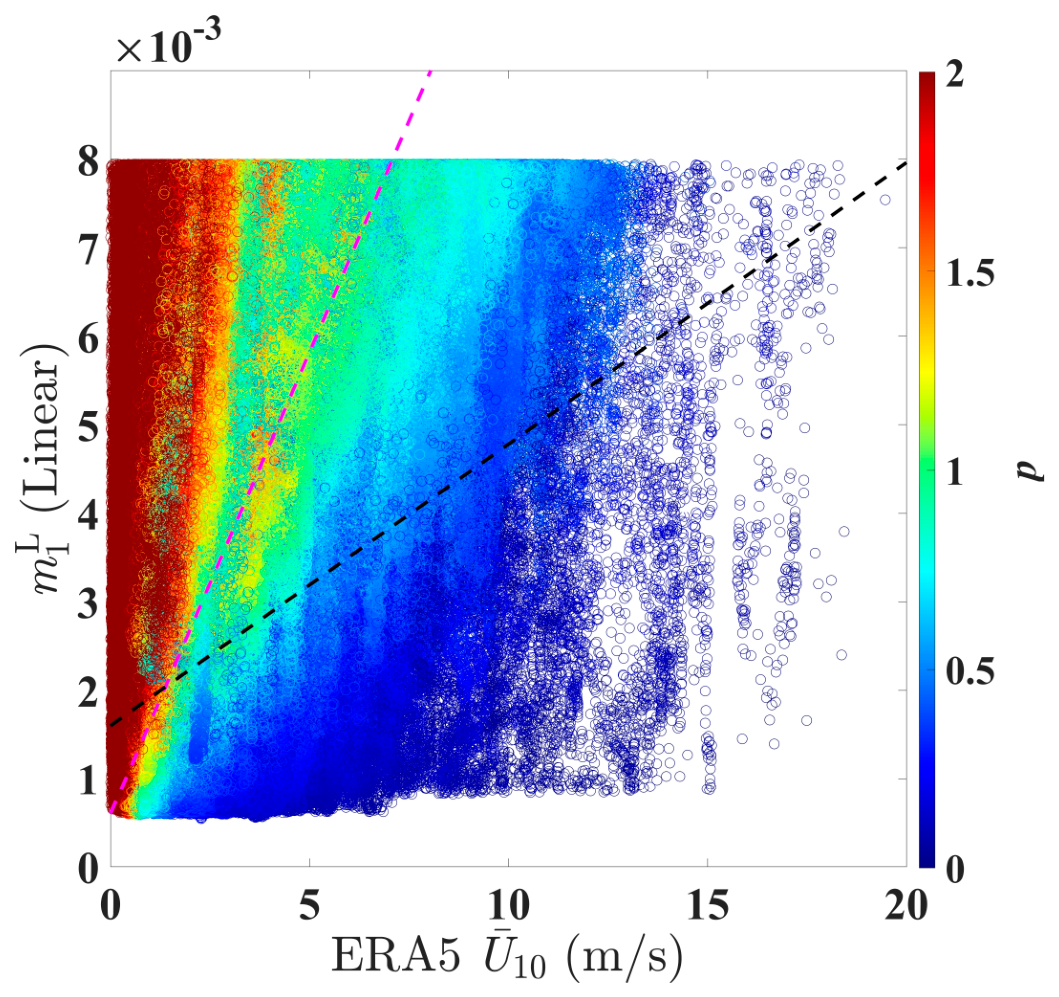
To determine the proportionality constant C, ERA5 reanalysis wind speeds were spatially interpolated to the geographic center of each SAR sub-image and matched with Equation (A7). Figure A1 presents the scatter distribution of ERA5 U ¯ 10 versus m 1 L , with the color scale indicating the ratio p between the m 1 L and the CMOD5.N-simulated value. Under ideal conditions, this ratio should equal unity (p = 1). Deviations indicate the presence of additional factors affecting sea-surface roughness: p > 1 suggests roughness enhancement (e.g., due to swell or bright targets), while p < 1 indicates roughness suppression (e.g., due to surface films).
Figure A1. Scatter distribution of ERA5 U ¯ 10 and m 1 L . The color scale represents the ratio p of m 1 L to the CMOD5.N-simulated value under linear units. The magenta dashed line represents m 1 L = 1.04 U ¯ 10 + 0.6 × 10 3 , and the black dashed line represents m 1 L = 3.18 U ¯ 10 + 16 × 10 4 .
Jmse 14 01555 g0a1
Through empirical fitting, the constant was determined to be C = 0.2. As illustrated in Figure A1, the magenta dashed line is m 1 L = 1.04 U ¯ 10 + 0.6 × 10 3 (clean surface threshold) and the black dashed line is m 1 L = 3.18 U ¯ 10 + 16 × 10 4 (slick surface threshold). Points above the magenta dashed line correspond to clean-sea-surface conditions, while points below the black dashed line indicate the presence of dark spots. Thus,
m 1 L > ( 1.04 U ¯ 10 + 6 )   × 10 3   for   clean   surface < ( 3.18 U ¯ 10 + 16 )   × 10 4   for   slick   surface  
In addition, oil spills in VV-polarized SAR imagery typically exhibit σ0 values below −21 dB [29]. Based on this constraint, sub-images satisfying the slick surface condition in Equation (A8) were extracted, and their joint probability density distribution in m1-m2 space was estimated using kernel density estimation (KDE), as shown in Figure A2a. Similarly, sub-images satisfying the clean surface condition were extracted and their m1-m2 probability density was computed (Figure A2b).
The black line in Figure A2 represents the optimal discriminant boundary separating dark spots from clean-sea-surface conditions, derived from the probability density distributions:
m 2 = 1.5 m 1 19
Therefore, the criterion for identifying dark spots in SAR imagery is:
m 2 1.5 m 1 19
Figure A2. Kernel density estimation of m1-m2 for (a) slick surface conditions ( m 1 L < 3.18 U ¯ 10 + 16 × 10 4 ) and (b) clean surface conditions ( m 1 L > 1.04 U ¯ 10 + 6 × 10 3 ). The black line is the optimal discriminant boundary (m2 = 1.5m1 − 19).
Jmse 14 01555 g0a2

References

  1. Monaldo, F.M.; Thompson, D.R.; Beal, R.C.; Pichel, W.G.; Clemente-Colon, P. Comparison of SAR-derived wind speed with model predictions and ocean buoy measurements. IEEE Trans. Geosci. Remote Sens. 2001, 39, 2587–2600. [Google Scholar] [CrossRef] [Scilit]
  2. Zhang, B.; Perrie, W.; He, Y. Wind speed retrieval from RADARSAT-2 quad-polarization images using a new polarization ratio model. J. Geophys. Res. Ocean. 2011, 116, C08008. [Google Scholar] [CrossRef] [Scilit]
  3. Valenzuela, G.R. Theories for the interaction of electromagnetic and oceanic waves—A review. Bound.-Layer Meteorol. 1978, 13, 61–85. [Google Scholar] [CrossRef] [Scilit]
  4. Quilfen, Y.; Chapron, B.; Collard, F.; Vandemark, D. Relationship between ERS scatterometer measurement and integrated wind and wave parameters. J. Atmos. Ocean. Technol. 2004, 21, 368–373. [Google Scholar] [CrossRef] [Scilit]
  5. Stopa, J.E.; Mouche, A.A.; Chapron, B.; Collard, F. Sea state impacts on wind speed retrievals from C-band radars. IEEE J. Sel. Top. Appl. Earth Obs. Remote Sens. 2017, 10, 2147–2155. [Google Scholar] [CrossRef] [Scilit]
  6. Li, H.; Mouche, A.A.; Stopa, J.E. Impact of sea state on wind retrieval from Sentinel-1 wave mode data. IEEE J. Sel. Top. Appl. Earth Obs. Remote Sens. 2019, 12, 559–566. [Google Scholar] [CrossRef] [Scilit]
  7. Wang, H.; Zhu, J.; Huang, X.; Chen, C.; Zhao, Y. Assessment of the swell impact on HY-2 SCAT wind products. In Proceedings of the Remote Sensing of the Ocean, Sea Ice, Coastal Waters, and Large Water Regions, Amsterdam, The Netherlands, 24–25 September 2014. [Google Scholar]
  8. Plagge, A.M.; Vandemark, D.; Chapron, B. Examining the impact of surface currents on satellite scatterometer and altimeter ocean winds. J. Atmos. Ocean. Technol. 2012, 29, 1776–1793. [Google Scholar] [CrossRef] [Scilit]
  9. Zhao, X.; Lin, W.; Wang, Z.; He, Y. Effects of sea surface temperature on the CFOSAT scatterometer measurements. Chin. J. Space Sci. 2023, 43, 190–198. [Google Scholar] [CrossRef] [Scilit]
  10. Marghany, M. Nonlinear Ocean Dynamics: Synthetic Aperture Radar; Elsevier: Amsterdam, The Netherlands, 2021. [Google Scholar]
  11. Hersbach, H. Comparison of C-band scatterometer CMOD5.N equivalent neutral winds with ECMWF. J. Atmos. Ocean. Technol. 2010, 27, 721–736. [Google Scholar] [CrossRef] [Scilit]
  12. Li, X.; Li, X.; Ren, Y.; Wu, K.; Li, C. Sea Surface Wind Speed Retrieval with a Dual-Branch Feature-Fusion Network Using GaoFen-3 Series SAR Data. Remote Sens. 2026, 18, 971. [Google Scholar] [CrossRef] [Scilit]
  13. Portabella, M.; Stoffelen, A.; Johannessen, J.A. Toward an optimal inversion method for synthetic aperture radar wind retrieval. J. Geophys. Res. Ocean. 2002, 107, 1–13. [Google Scholar] [CrossRef] [Scilit]
  14. Mouche, A.A.; Vincent, P. Sentinel-1 Ocean Wind Fields (OWI) Algorithm Definition; Version 2.0; European Space Agency: Paris, France, 2019; Available online: https://sentinels.copernicus.eu/documents/247904/3861173/Sentinel-1-Ocean-Wind-Fields-OWI-ATBD.pdf (accessed on 24 May 2023).
  15. Xu, Q.; Li, Y.; Li, X.; Zhang, Z.; Cao, Y.; Cheng, Y. Impact of ships and ocean fronts on coastal sea surface wind measurements from the Advanced Scatterometer. IEEE J. Sel. Top. Appl. Earth Obs. Remote Sens. 2018, 11, 2162–2169. [Google Scholar] [CrossRef] [Scilit]
  16. Jang, J.C.; Park, K.A.; Mouche, A.A.; Chapron, B.; Lee, J. Validation of sea surface wind from Sentinel-1A/B SAR data in the coastal regions of the Korean Peninsula. IEEE J. Sel. Top. Appl. Earth Obs. Remote Sens. 2019, 12, 2513–2529. [Google Scholar] [CrossRef] [Scilit]
  17. Ribal, A.; Young, I.R. 33 years of globally calibrated wave height and wind speed data based on altimeter observations. Sci. Data 2019, 6, 77. [Google Scholar] [CrossRef] [Scilit] [PubMed]
  18. Mears, C.; Lee, T.; Ricciardulli, L.; Wang, X.; Wentz, F. RSS Cross-Calibrated Multi-Platform (CCMP) 6-Hourly Ocean Vector Wind Analysis on 0.25 Degree Grid; Remote Sensing Systems: Santa Rosa, CA, USA, 2020. [Google Scholar] [CrossRef] [Scilit]
  19. Climate Data Store. ERA5 Hourly Data on Single Levels from 1940 to Present; Copernicus Climate Change Service (C3S): Bonn, Germany, 2024. [Google Scholar] [CrossRef]
  20. Wessel, P.; Smith, W.H.F. A global, self-consistent, hierarchical, high-resolution shoreline database. J. Geophys. Res. Solid Earth 1996, 101, 8741–8743. [Google Scholar] [CrossRef] [Scilit]
  21. Ali, I.; Cao, S.; Naeimi, V.; Paulik, C.; Wagner, W. Methods to remove the border noise from Sentinel-1 synthetic aperture radar data: Implications and importance for time-series analysis. IEEE J. Sel. Top. Appl. Earth Obs. Remote Sens. 2018, 11, 777–786. [Google Scholar] [CrossRef] [Scilit]
  22. Miranda, N.; Meadows, P.; Piantanida, R.; Recchia, A.; Small, D.; Schubert, A.; Vincent, P.; Geudtner, D.; Navas-Traver, I.; Vega, F.C. The Sentinel-1 constellation mission performance. In Proceedings of the IEEE International Geoscience and Remote Sensing Symposium (IGARSS), Fort Worth, TX, USA, 23–28 July 2017. [Google Scholar]
  23. Sun, Y.; Li, X. Denoising Sentinel-1 extra-wide mode cross-polarization images over sea ice. IEEE Trans. Geosci. Remote Sens. 2021, 59, 2116–2131. [Google Scholar] [CrossRef] [Scilit]
  24. Park, J.W.; Won, J.S.; Korosov, A.A.; Babiker, M.; Miranda, N. Textural noise correction for Sentinel-1 TOPSAR cross-polarization channel images. IEEE Trans. Geosci. Remote Sens. 2019, 57, 4040–4049. [Google Scholar] [CrossRef] [Scilit]
  25. Cox, C.; Munk, W. Measurement of the roughness of the sea surface from photographs of the Sun’s glitter. J. Opt. Soc. Am. 1954, 44, 838–850. [Google Scholar] [CrossRef] [Scilit]
  26. Brekke, C.; Solberg, A.H.S. Oil spill detection by satellite remote sensing. Remote Sens. Environ. 2005, 95, 1–13. [Google Scholar] [CrossRef] [Scilit]
  27. Jones, A.T.; Thankappan, M.; Logan, G.A.; Kennard, J.M.; Smith, C.J.; Williams, A.K.; Lawrence, G.M. Coral spawn and bathymetric slicks in synthetic aperture radar (SAR) data from the Timor Sea, northwest Australia. Int. J. Remote Sens. 2005, 27, 2063–2069. [Google Scholar] [CrossRef] [Scilit]
  28. Fung, A.K.; Pan, G.W. An integral equation method for rough surface scattering. In Proceedings of the International Symposium on Multiple Scattering of Waves in Random Media and Random Surfaces, Los Angeles, PA, USA, 29 July–2 August 1985. [Google Scholar]
  29. Dong, Y.; Liu, Y.; Hu, C.; MacDonald, I.R.; Lu, Y. Chronic oiling in global oceans. Science 2022, 376, 1300–1304. [Google Scholar] [CrossRef] [Scilit] [PubMed]
Figure 1. Spatial coverage of SAR images. (Left): a total of 4193 VV-polarized and 3775 VH-polarized SAR images over the Gulf of Mexico from 2016 to 2019. (Right): a total of 2055 VV-polarized SAR images acquired around Taiwan Island from 2014 to 2024. Blue pentagrams and triangles represent the locations of buoys measuring wind at 10 m and 3 m height above sea level, respectively.
Jmse 14 01555 g001
Figure 2. Schematic representation of border noise in SAR imagery. (a) VV-polarized SAR image acquired at 12:09 UTC on 16 January 2016, with the red-circled area enlarged in (c,d); (b) corresponding VH-polarized SAR image, with the red-circled area enlarged in (e,f). Panels (c,e) display the original SAR images, while panels (d,f) show the images after 5-look multi-look processing.
Jmse 14 01555 g002
Figure 3. Detection of border noise in IW mode SAR imagery. (a) VV-polarized SAR image acquired at 00:02 UTC on 15 May 2016. (b) VH-polarized SAR image acquired at 00:01 UTC on 28 January 2016. Panels (c,d) show the m1-m2 distributions derived from (a) and (b), respectively. Panels (e,f) show the m1-m2 distributions derived from all VV-polarized and VH-polarized SAR images covering the Gulf of Mexico, with the color scale indicating point number. Data points corresponding to the detected border noise are indicated by green dashed ellipses in panels (c,d), with the corresponding pixels marked by small red circles in panels (a,b).
Jmse 14 01555 g003
Figure 4. Detection of inter-swath stripe noise in IW mode SAR imagery. (a) VV-polarized SAR image acquired at 00:07 UTC on 27 January 2017. (b) Corresponding VH-polarized SAR image. Panels (c,d) show the m1-m2 distributions derived from (a) and (b), respectively. Panels (e,f) show the m1-m2 distributions derived from all VV- and VH-polarized SAR images covering the Gulf of Mexico. Data points corresponding to the detected noise are indicated by green dashed ellipses in panels (c,d), with the corresponding pixels marked by small red circles in panels (a,b).
Jmse 14 01555 g004aJmse 14 01555 g004b
Figure 5. Detection of land contamination in IW mode SAR imagery. (a) VV-polarized SAR image acquired at 23:53 UTC on 22 January 2016. (b) Corresponding VH-polarized SAR image. Panels (c,d) show the m1-m2 distributions derived from (a) and (b), respectively. Panels (e,f) show the m1-m2 distributions derived from all VV- and VH-polarized SAR images covering the Gulf of Mexico. Data points corresponding to the detected coastal land residuals are indicated by green dashed ellipses in panels (c,d), with the corresponding pixels marked by small red circles in panels (a,b).
Jmse 14 01555 g005
Figure 6. Detection of bright targets in IW mode SAR imagery. (a) VV-polarized SAR image acquired at 12:06 UTC on 16 January 2016. (b) Corresponding VH-polarized SAR image. Panels (c,d) show the m1-m2 distributions derived from (a) and (b), respectively. Panels (e,f) show the m1-m2 distributions derived from all VV- and VH-polarized SAR images covering the Gulf of Mexico. Data points corresponding to the detected bright targets are indicated by green dashed ellipses in panels (c,d), with the corresponding pixels marked by small red circles in panels (a,b).
Jmse 14 01555 g006aJmse 14 01555 g006b
Figure 7. Detection of dark spots in VV-polarized SAR imagery with IW mode. (a) VV-polarized SAR image captured at 23:36 UTC on 30 April 2017, with wind speed ranging from 0 to 4 m/s. (b) Corresponding detection result using the criterion m 2 1.5 m 1 19 , with dark spots highlighted in red.
Jmse 14 01555 g007
Figure 8. Classification summary for (a) VV-polarized and (b) VH-polarized Sentinel-1 IW mode SAR imagery in the m1-m2 space.
Jmse 14 01555 g008
Figure 9. Comparison of SAR-derived wind speeds with buoy-measured wind speeds before and after quality control (QC). The first and second panels show the validation against native 10 m buoy observations before QC (n = 859, RMSE = 1.5 m/s, MBE = −0.3 m/s) and after QC (n = 737, RMSE = 1.5 m/s, MBE = −0.3 m/s), respectively. The last two panels show the validation against nearshore buoy observations measured at 3 m and converted to 10 m equivalent neutral winds before QC (RMSE = 3.2 m/s, MBE = −1.5 m/s) and after QC (RMSE = 2.1 m/s, MBE = −1.1 m/s), respectively. The black solid line represents the 1:1 line, and the red dashed line represents the fitted regression line.
Jmse 14 01555 g009
Figure 10. Preliminary analysis of EW mode SAR imagery based on the relationship of m1 and m2. (a) Original VV-polarized image acquired at 03:32 UTC on 31 August 2018. (b) σ0 variation along the range direction of (a). (c) m1-m2 distribution derived from (a). (d) Corresponding original VH-polarized image. (e) σ0 variation along the range direction of (d). (f) m1-m2 distribution derived from (d), revealing a ~1 dB offset between EW1 and other sub-swaths. (g) The VH-polarized image after σ0 offset correction. (h) σ0 variation along the range direction of (g). (i) m1-m2 distribution derived from (g).
Jmse 14 01555 g010
Table 1. Classification summary for IW mode.
VVExpressionVHExpressionMain Features
m 2 8 m 1 + 185 m 1 40   and   m 2 1.1 m 1 26 Border noise
2 m 1 + 3 m 2 < 8 m 1 + 185 m 2 > 1.1 m 1 10 Bright targets
m 2 2 m 1 8 m 1 > 40   and   m 2 2 m 1 8 Inter-swath stripe noise
m 2 < 8 m 1 + 185   and   m 2 1.5 m 1 19 --Dark spots
m 2 < 8 m 1 + 185   and   2 m 1 3 m 2 < 2 m 1 + 3 2 m 1 3 m 2 < 1.1 m 1 10 Land contamination
m 2 < 8 m 1 + 185 ,
m 2 > 1.5 m 1 19 ,   and   2 m 1 8 < m 2 < 2 m 1 3
m 1 > 40   and   2 m 1 8 < m 2 < 2 m 1 3 Clean sea surface
Table 2. Contributions of individual quality-control filters to SAR-derived wind speed validation against nearshore buoy observations.
Buoy SubsetQC ConfigurationRetained Collocations, nMBE (m/s), 95% CIRMSE (m/s), 95% CI
Height-adjusted 3 m nearshore buoy windsNo QC1807−1.5, [−1.68, −1.42]3.2, [2.88, 3.57]
Border noise only1806−1.6, [−1.69, −1.43]3.2, [2.87, 3.57]
Bright targets only1796−1.5, [−1.58, −1.35]2.9, [2.65, 3.13]
Inter-swath stripe noise only1807−1.5, [−1.68, −1.42]3.2, [2.88, 3.57]
Dark spots only1794−1.6, [−1.69, −1.43]3.2, [2.89, 3.60]
Land contamination only1580−1.2, [−1.34, −1.11]2.6, [2.25, 3.05]
Full QC1555−1.1, [−1.23, −1.05]2.1, [2.00, 2.26]
Note: CI represents ‘confidence interval’.
Disclaimer/Publisher’s Note: The statements, opinions and data contained in all publications are solely those of the individual author(s) and contributor(s) and not of MDPI and/or the editor(s). MDPI and/or the editor(s) disclaim responsibility for any injury to people or property resulting from any ideas, methods, instructions or products referred to in the content.