Influence of Bilateral WIG Effect on Oscillating Hydrofoil Energy Harvesting Performance and Experimental Suggestions

Abstract

The oscillating hydrofoil represents a promising tidal energy harvesting device, but its hydrodynamic behavior and energy harvesting performance can be significantly affected by the wing-in-ground (WIG) effect under near-wall conditions. The present work establishes a two-dimensional numerical model that accounts for bilateral WIG effect to investigate the effect of three key parameters, namely the dimensionless wall distance ($H^{\ast }$), the Reynolds number ($Re$), and the reduced oscillation frequency ($f^{\ast }$) on energy harvesting performance. The formation, shedding, and reattachment of the leading-edge vortex (LEV) are analyzed to clarify the underlying hydrodynamic mechanisms. The results demonstrate that the WIG effect notably enhances the energy harvesting efficiency of the oscillating hydrofoil. At $Re=5\times {10}^5$ and $f^{\ast }=0.14$, the maximum energy harvesting efficiency reaches 69.6% at $H^{\ast }=2$, representing an improvement of 84.1% over the reference efficiency of 37.8% at the negligible WIG reference condition of $H^{\ast }=40$. As $H^{\ast }$ increases, the hydrodynamic performance gradually approaches that of the unconfined hydrofoil. Based on the predefined 5% efficiency-deviation criterion, the WIG effect becomes negligible at approximately $H^{\ast }=9$. The sensitivity to the WIG effect increases at higher oscillation frequencies, whereas its dependence on $Re$ is non-monotonic, decreasing up to $Re=4.5\times {10}^5$ and increasing thereafter. Finally, the four-component Gaussian mixture model (GMM) is employed to construct a prediction model for the wall distance at which the WIG effect becomes negligible under different combinations of the Reynolds number and the oscillation frequency. The model achieves an $RMSE$ of 1.991 and an $R^2$ of 0.667. These results quantify the effective range of the bilateral WIG effect and provide a practical criterion for reducing wall interference in relevant experiments.

1. Introduction

The escalating contradiction between global energy shortages and energy demand growth has become ever more prominent. This realistic background has driven the focus of energy development to gradually shift from traditional fossil fuels to renewable energy sources such as marine energy and wind energy, which boast abundant reserves but remain insufficiently exploited [1]. As a form of marine renewable energy, tidal energy holds broad application prospects due to its higher resource reserves and larger power density [2,3]. Among the technologies, the oscillating hydrofoil tidal energy harvesting device possesses prominent advantages, including higher space utilization, lower flow velocity requirements, and environmental friendliness. The oscillating hydrofoil tidal energy harvesting device has garnered extensive scholarly interest in recent years [4,5].

Oscillating hydrofoil researchers conducted parametric studies through numerical simulations and experiments. Lindsey [6] investigated the flow characteristics of the oscillating hydrofoil under the Reynolds number $Re={10}^6$ and $Re=2\times {10}^4$. The findings showed that the power coefficient and the total energy harvesting efficiency at the higher Reynolds number are significantly higher than those at the lower Reynolds number. Dumas and Kinsey [7,8] and Bernardo et al. [9] further confirmed through experiments that the energy harvesting efficiency increases with the increasing Reynolds number. Kinsey et al. [10] and Veilleux et al. [11,12] experimentally validated the reliability of numerical models, emphasizing that vortex shedding caused by stall flutter plays a critical role in the dynamics under higher-Reynolds-number conditions. Simpson [13] introduced the reduced frequency to replace the Strouhal number based on oscillating amplitude, parameterizing the experimental data. Results showed that it better unifies efficiency distributions across different amplitudes, with the maximum energy harvesting efficiency region concentrated at $f^{*}=0.12–0.15$. Buchner et al. [14], Hoerner et al. [15] and Xu et al. [16] indicated that reducing the oscillation frequency decreases the effective angle of attack. This affects vortex generation, shedding and reattachment, ultimately altering the energy harvesting efficiency. Zhu [17,18] investigated the correlation between energy harvesting efficiency and wake stability. The finding showed that the foil-wake resonance is induced when the reduced frequency of the oscillating hydrofoil is about 0.15, which in turn optimizes the system’s energy harvesting efficiency. Taylor et al. [19], and Ashraf et al. [20] also demonstrated that the oscillating hydrofoil tidal energy harvesting device exhibits superior energy harvesting performance when $f^{*}=0.10–0.25$. Sun et al. [21] numerically found that the oscillation frequency significantly affects the energy harvesting performance of the oscillating hydrofoil by regulating vortex shedding and pressure distribution. Lower frequencies favor vortexes reused again while higher frequencies enhance heave force via pressure difference. Liu et al. [22] systematically summarized the relationship between the peak of energy harvesting efficiency and the oscillation frequency under various parametric conditions.

The wing-in-ground effect is a fluid dynamics effect arising from the interaction between the foil and the solid boundary when operating close to the latter. He et al. [23] proposed that a Venturi channel forms when a hydrofoil approaches the solid boundary. This leads to a good timing of vortex–foil interactions and significantly increases the energy harvesting power. Su et al. [24] and Wu et al. [25] investigated the energy harvesting performance of the oscillating hydrofoil under the wing-in-ground effect. Compared to the unconstrained condition, the energy harvesting efficiency is moderately improved with the one-wall confinement while the two-wall confinement can significantly enhance it. Further studies by Wang et al. [26] and Zhu et al. [27] demonstrated that the beneficial influence of the wing-in-ground effect on energy harvesting efficiency becomes more pronounced as the oscillation frequency and angle of attack increase. Mo et al. [28] primarily attributed this energy harvesting efficiency gain to increased pressure on the hydrofoil’s lower surface from the wing-in-ground effect. Yang et al. [29] in turn analyzed experimental data, successfully isolating the wing-in-ground effect’s impact on energy harvesting. Zhao et al. [30] investigated a tandem oscillating hydrofoil system considering the wing-in-ground effect. The result shows the energy harvesting efficiency of this system can be increased by 66.7% compared to a single hydrofoil in unconfined flow. Ma et al. [31] developed a coupled model incorporating both flexible deformation and dynamic wing-in-ground effect, confirming the positive role of the wing-in-ground effect in enhancing energy harvesting. However, Karakas et al. [32] experimentally noted that excessive proximity between the hydrofoil and the solid boundary causes flow blockage and adverse interference. This instead reduced energy harvesting efficiency.

In summary, existing research has confirmed that the wing-in-ground effect is a key factor influencing the energy harvesting performance of the oscillating hydrofoil. It exhibits a complex coupling mechanism with parameters such as the Reynolds number and the oscillation frequency, which remain to be further clarified. The present work establishes a numerical model accounting for the wing-in-ground effect and performs simulation analyses. It focuses on analyzing the coupled effect of the dimensionless wing-in-ground distance, the Reynolds number, and the oscillation frequency on energy harvesting performance. The four-component Gaussian mixture model is employed to establish a mapping relationship between these key parameters and the wing-in-ground effect. Thereby providing theoretical support for avoiding the wing-in-ground effect’s interference in oscillating hydrofoil experimental design.

2. Computational Model and Method

The schematic diagram of the two-dimensional oscillating hydrofoil is shown in Figure 1. The oscillating hydrofoil employs a NACA0015 hydrofoil with a chord length of $c$, $c=0.25\mathrm{m}$. $U_{\infty }$ represents the velocity of the incoming flow. The Reynolds number is defined as $Re=\rho U_{\infty }c/\mu$, where $\rho$ is the fluid density and $\mu$ is the fluid dynamic viscosity [9,28,29]. $H$ denotes the distance from the pitching axis to the wall. The heaving and pitching motions follow the sinusoidal formulations commonly adopted in oscillating hydrofoil energy harvesting studies [8,9,13].

$$h\left(t\right)=h_{0}sin\left(2\pi ft\right)$$

(1)

$$\theta \left(t\right)={\theta }_{0}sin\left(2\pi ft+\phi \right)$$

(2)

where $h_0$ and ${\theta }_0$ respectively denote the heave and pitch amplitudes; $f$ denotes the dimensional oscillation frequency expressed in hertz (Hz), whereas $f^{*}=fc/U_{\infty }$ denotes the dimensionless reduced oscillation frequency; $\phi$ represents the phase difference between the heaving and pitching motions, $\phi ={\displaystyle \frac{\pi }{2}}$.

The lift coefficient $C_L$ and moment coefficient $C_M$ are expressed as [9,24]:

$$C_L={\displaystyle \frac{F_L\left(t\right)}{0.5\rho U_{\infty }^{2}cb}}$$

(3)

$$C_M={\displaystyle \frac{M\left(t\right)}{0.5\rho U_{\infty }^2{c}^{2}b}}$$

(4)

where $F_L\left(t\right)$ denotes the instantaneous lift force, and $M\left(t\right)$ denotes the instantaneous pitching moment, $b$ is the span length of the hydrofoil, with a value of $b=1 \mathrm{m}$.

The instantaneous output power of the hydrofoil is defined as the sum of the heaving power $P_L\left(t\right)$ and the pitching power $P_M\left(t\right)$ [8,9,18], which are expressed as:

$$P_L\left(t\right)=F_L\left(t\right)\stackrel{·}{h}\left(t\right)$$

(5)

$$P_M\left(t\right)=M\left(t\right)\stackrel{·}{\theta }\left(t\right)$$

(6)

$$P\left(t\right)=P_L\left(t\right)+P_M\left(t\right)=F_L\left(t\right)\stackrel{·}{h}\left(t\right)+M\left(t\right)\stackrel{·}{\theta }\left(t\right)$$

(7)

where $\stackrel{·}{h}\left(t\right)$ is the instantaneous heaving velocity, and $\stackrel{·}{\theta }\left(t\right)$ is the instantaneous pitching angular velocity.

The average power $\overline{P}$ is given by:

$$\overline{P}=\overline{P_L}+\overline{P_M}={\displaystyle \frac{1}{T}}{\displaystyle {\int }_t^{t+T}{P}_L\left(t\right)dt}+{\displaystyle \frac{1}{T}}{\displaystyle {\int }_t^{t+T}{P}_M\left(t\right)dt}$$

(8)

where $\overline{P_L}$ and $\overline{P_M}$ are the average heaving power and average pitching power, $T$ is the time of a cycle [9,13,18].

The power coefficient $C_P\left(t\right)$ is given by:

$$C_P\left(t\right)={\displaystyle \frac{P\left(t\right)}{0.5\rho U_{\infty }^{3}c}}=C_{PL}\left(t\right)+C_{PM}\left(t\right)$$

(9)

where $C_{PL}\left(t\right)$ and $C_{PM}\left(t\right)$ denote the instantaneous heaving and pitching power coefficients, respectively.

$$C_{PL}\left(t\right)={\displaystyle \frac{C_L\left(t\right)\stackrel{·}{h}\left(t\right)}{U_{\infty }}}$$

(10)

$$C_{PM}\left(t\right)={\displaystyle \frac{c{C}_M\left(t\right)\stackrel{·}{\theta }\left(t\right)}{U_{\infty }}}$$

(11)

The cycle-average power coefficient $\overline{C_p}$ is consequently defined as [9,10,25]:

$$\overline{C_p}={\displaystyle \frac{\overline{P}}{0.5\rho {U^3}_{\infty }c}}={\displaystyle \frac{1}{T}}{\displaystyle {\int }_t^{t+T}{C}_P\left(t\right)dt}=\overline{C_{PL}}+\overline{C_{PM}}$$

(12)

The total energy of the fluid flowing through the region is expressed as follows:

$$P_a=0.5\rho {U^3}_{\infty }A$$

(13)

where $A$ is the effective swept area of the oscillating hydrofoil, $A=h_{m}b$. The effective swept height $h_m$ is determined by the coupled heave–pitch motion and the position of the pitching axis as illustrated in Figure 1 [24,29]. It can be expressed as:

$$h_m=\max \left\{\begin{array}{l}{h}_0\sin (2\pi ft)+c_1\sin (2\pi ft+\phi )\\ h_0\sin (2\pi ft)-c_2\sin (2\pi ft+\phi )\end{array}\right\}$$

(14)

where $c_1$ and $c_2$ represent the distances from the pitching axis to the trailing edge and the leading edge, respectively, with $c_1={\displaystyle \frac{2}{3}}c$ and $c_2={\displaystyle \frac{1}{3}}c$.

The energy conversion efficiency $\eta$ is expressed as [8,9,13,18,29]:

$$\eta ={\displaystyle \frac{\stackrel{-}{P}}{P_a}}={\displaystyle \frac{\stackrel{-}{P}}{0.5\rho U_{\infty }^3{h}_m}}=\overline{C_p}{\displaystyle \frac{c}{h_m}}$$

(15)

For the numerical simulation of two-dimensional incompressible flow, the mathematical model of the present study are the Navier–Stokes equations. The equations are formulated as the continuity equation and the momentum equation, expressed as follows:

$$\nabla \mathit{u}=0$$

(16)

$${\displaystyle \frac{d\mathit{u}}{dt}}+\left(\mathit{u}\cdot \nabla \right)\mathit{u}=-{\displaystyle \frac{1}{\rho }}\nabla \mathit{p}+{\displaystyle \frac{\mu }{\rho }}{\nabla }^2\mathit{u}$$

(17)

where $\mathit{u}=\left(u,v\right)$ is the fluid velocity vector, and $\mathit{p}$ is the pressure [9,10,28].

3. Numerical Model

The two-dimensional incompressible Unsteady Reynolds-Averaged Navier–Stokes (URANS) equations are solved using a pressure-based transient finite-volume formulation. Turbulence closure is provided by the one-equation Spalart–Allmaras (SA) model [2,5,23,28]. The SA model is adopted because previous SA-based URANS simulations of high-Reynolds-number oscillating hydrofoils provide satisfactory predictions of integral turbine performance when compared with experimental measurements. In particular, Kinsey and Dumas examined the influence of different turbulence closures, including the SA, standard k–ω, and k–ω SST models, in related oscillating hydrofoil simulations [10]. These studies provide a relevant methodological basis for adopting the SA model in the present two-dimensional parametric investigation. The SA model is used for all cases investigated in Section 4.1, Section 4.2 and Section 4.3. Section 4.4 extends the investigated Reynolds number range to the lower-Reynolds-number regime; therefore, the flow model selection and the corresponding model sensitivity assessment are described separately in that section. The Semi-Implicit Method for Pressure-Linked Equations (SIMPLE) algorithm is used for pressure–velocity coupling. The pressure term is discretized using the second-order scheme, whereas the momentum and modified turbulent-viscosity equations are discretized using the second-order upwind scheme [2,5].

The computational domain and mesh structure are illustrated in Figure 2. The computational domain is a rectangular region with a size of 80c × 60c, where c denotes the chord length of the oscillating hydrofoil. The left boundary is defined as a velocity inlet, and the right boundary is defined as a pressure outlet. The upper and lower boundaries are modeled as stationary, smooth, no-slip walls. The incoming flow velocity is $U_{\infty }=2\mathrm{m}/\mathrm{s}$, corresponding to the Reynolds number of $Re=5\times {10}^5$. The heave amplitude and pitch amplitudes are set to $h_0=0.25\mathrm{m}$ and ${\theta }_0=75°$, respectively. The hydrofoil surface is modeled as a smooth, rigid, moving no-slip wall, whose translational and rotational velocities follow the prescribed heaving and pitching motions. To resolve the near-wall velocity gradients, wall-normal structured quadrilateral boundary-layer meshes are generated along the hydrofoil surface and both confining walls. The first layer mesh height, number of layers, and growth ratio are set to 1.1 × 10⁻⁵, 25, and 1.2, respectively. These mesh parameters are selected to a target value of $y^{+}\le 1$ throughout the simulations. A 4c × 2c rectangular region surrounding the hydrofoil is defined as the transformation domain. The prescribed heaving and pitching motions are imposed according to Equations (1) and (2). Spring-based smoothing and local remeshing are used to update the computational mesh at each time step. Only the unstructured cells in the transformation domain are allowed to deform and be regenerated, whereas the outer structured region remains stationary. Local remeshing is activated when the cell skewness in the transformation domain exceeds 0.6 or when its characteristic cell size falls outside 0.0021–0.007 m. Extend unstructured triangular mesh domain by $c$ in all directions around it to achieve the mesh size transition between the transformation domain and the outer computational domain.

To ensure numerical accuracy and computational reliability, mesh-independence and time-step-independence analyses are conducted. The corresponding quantitative results are summarized in

Table 1. Independence verification of the grid number and the time step.

Object	Mesh Number	Time-Step Size (s)	${\mathit{C}}_{\mathit{L}\mathbf{max}}$	${\mathit{C}}_{\mathit{L}\mathbf{max}}$ Difference	$\overline{{\mathit{C}}_{\mathit{P}}}$	$\overline{{\mathit{C}}_{\mathit{P}}}$ Difference
The mesh-independence verification	$1.36\times {10}^5$	0.001	2.736	−1.1%	0.958	−0.3%
	$2.94\times {10}^5$	0.001	2.767	-	0.961	-
	$4.23\times {10}^5$	0.001	2.774	0.3%	0.962	0.1%
Time-step-independence verification	$2.94\times {10}^5$	0.002	2.680	−3.1%	0.943	−1.8%
	$2.94\times {10}^5$	0.001	2.767	-	0.961	-
	$2.94\times {10}^5$	0.0005	2.761	−0.2%	0.957	−0.4%

, while the instantaneous vorticity contours obtained using different grid resolutions and time-step sizes are compared in Figure 3.

As summarized in Table 1, increasing the mesh number from $2.94\times {10}^5$ to $4.23\times {10}^5$ results in differences of only 0.3% and 0.1% in the maximum lift coefficient ($C_{L\max }$) and the cycle-averaged power coefficient ($\overline{C_P}$), respectively. In addition, reducing the time step from 0.001 s to 0.0005 s changes these quantities by only 0.2% and 0.4%, respectively. These small deviations indicate that further spatial and temporal refinement provides only marginal improvements in the predicted hydrodynamic performance.

Figure 3 further provides qualitative support for this conclusion by comparing the instantaneous vorticity contours obtained using different mesh resolutions and time-step sizes. The dominant flow structures, including the leading-edge vortex, the separated shear layer, and the near-wake vortex pattern, remain nearly unchanged for the medium and fine mesh resolutions, as well as for the time-step sizes of 0.001 s and 0.0005 s. Only the coarsest mesh and the largest time-step produce slightly smoother local vortical structures, while the overall vortex evolution is still well preserved. Therefore, the mesh containing $2.94\times {10}^5$ cells and the time step size of 0.001 s are adopted for all subsequent simulations as an appropriate compromise between numerical accuracy and computational cost.

In total, 20 iterations are performed at each time step. Simulations are continued until a periodically converged state is achieved. At each time step, the scaled residuals of the continuity, momentum, and modified turbulent-viscosity equations are required to decrease below 10⁻⁶. In addition, periodic convergence is considered to be achieved when the relative difference in the cycle-averaged power coefficient ($\epsilon \overline{C_p}$) between two consecutive cycles is less than 1%. The statistics $n$ reported in this study are the fifth oscillation cycle.

$$\epsilon \overline{C_p}={\displaystyle \frac{\left|{\overline{C_p}}^n-{\overline{C_p}}^{n-1}\right|}{\left|{\overline{C_p}}^{n-1}\right|}}={\displaystyle \frac{\left|0.961-0.959\right|}{\left|0.959\right|}}\times 100\%=0.2\%<1\%.$$

(18)

The present simulation results are compared with those from Kinsey and Dumas [10]. As shown in Figure 4, the lift and moment coefficients exhibit excellent agreement in overall trends.

As shown in

Table 2. Comparisons of the present average results against the reference data by Kinsey and Dumas [10].

Quantity	Present Study	Reference	Relative Error
${C_L}_{\max }$	2.767	2.800	1.2%
$\overline{C_P}$	0.961	0.986	2.5%
$\eta$	37.8%	38.9%	2.8%

, quantitative validation is performed by comparing the peak lift coefficient, the cycle-average power coefficient, and the energy harvesting efficiency with the data reported by Kinsey and Dumas. The relative errors are 1.2%, 2.5%, and 2.8%, respectively, confirming the reliability of the numerical approach with acceptable accuracy.

4. Results and Discussion

This research aims to investigate the influence of the wing-in-ground (WIG) effect on the energy harvesting performance of the oscillating hydrofoil. The wall distance is one of the core factors governing the intensity of the WIG effect. In addition, variations in the oscillation frequency and the Reynolds number alter the flow field characteristics. Such alterations further modify the effect of the WIG effect. This research selects the above key parameters for systematic analysis. The selected reference parameters are presented in

Table 3. Reference parameters.

Parameters	${\mathit{h}}_0$	${\mathit{\theta }}_0$	$\mathit{\phi }$	${\mathit{H}}^{\ast }$	${\mathit{f}}^{*}$	$\mathit{R}\mathit{e}$
Value	$c$	75°	90°	9	0.14	$5\times {10}^5$

.

4.1. The Influence of the Dimensionless Wall Distance on Energy Harvesting Efficiency

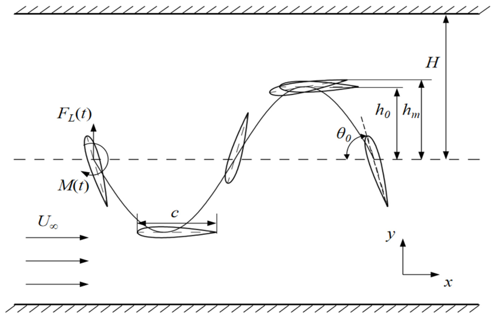
When the oscillating hydrofoil approaches the wall, the WIG effect is induced. This effect influences the motion behavior of the fluid, thereby regulating the mechanical characteristics of the oscillating hydrofoil surface and affecting its energy harvesting performance. To investigate the mechanism of the WIG effect, the dimensionless wall distance $H^{\ast }$ is investigated. A total of 20 cases are set up in this research. Among them, the parameters of 19 cases are uniformly selected within the range of $H^{\ast }\in [2,20]$. It is designed to cover the variation process of the WIG effect from strong to weak. $H^{\ast }=40$ serves as the reference case, under which the WIG effect is considered negligible.

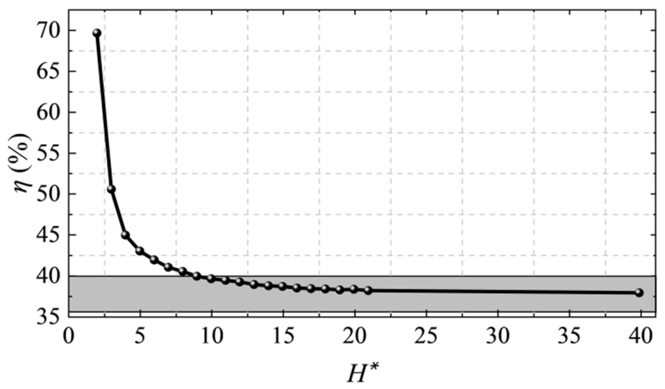
Figure 5 illustrates the variation in the energy harvesting efficiency of the oscillating hydrofoil with $H^{\ast }$. When $H^{\ast }=2$, the energy harvesting efficiency of the oscillating hydrofoil reaches as high as 69.6%. As $H^{\ast }$ increases, the energy harvesting efficiency exhibits a monotonically decreasing trend, and the rate of decline tends to stabilize. This phenomenon is consistent with the experimental work of Yang et al. [29], who isolated the contribution of the WIG effect and corroborated the conclusion that energy harvesting efficiency is governed by wall separation distance. The present results further indicate that bilateral confinement produces a substantial efficiency enhancement compared with the far-wall reference condition. And the relative efficiency deviation from the far-wall reference condition is characterized by the parameter $\alpha$. The WIG effect is considered negligible when $\alpha \le 5\%$.

$$\alpha ={\displaystyle \frac{{\eta }_n-{\eta }_{40}}{{\eta }_{40}}}\times 100\%$$

(19)

When $H^{\ast }=9$, the energy harvesting efficiency reaches 39.7%, which is 5.0% higher than the 37.8% efficiency observed at $H^{\ast }=40$. Moreover, when $H^{\ast }\ge 9$, the energy harvesting efficiency changes slowly. Therefore, in this research, the energy harvesting efficiency deviation of less than 5% can be regarded as being unaffected by the WIG effect.

Figure 5. Energy harvesting efficiency under different $H^{\ast }$.

Figure 5. Energy harvesting efficiency under different $H^{\ast }$.

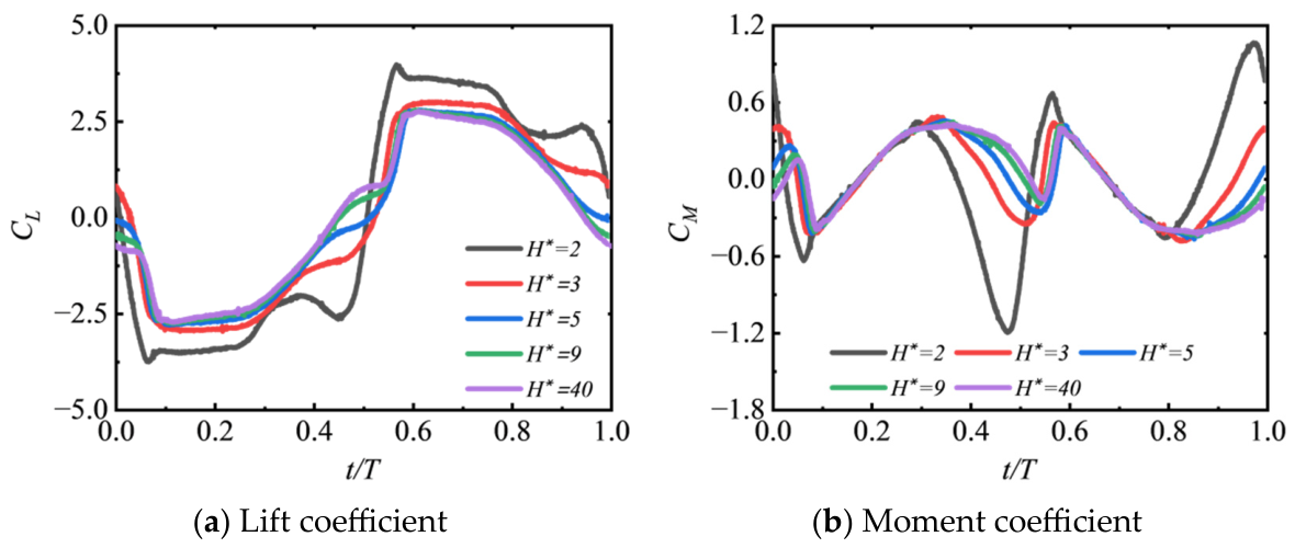
Based on Figure 5, five typical cases with $H^{\ast }$ = 2, 3, 5, 9, 40 are selected for investigation. Figure 5 presents the lift coefficient and moment coefficient of the oscillating hydrofoil under different $H^{\ast }$. Due to the symmetry of the oscillating hydrofoil’s oscillating motion, the lift and moment coefficient exhibit symmetric distribution over one full cycle. Therefore, this research only analyzes the first half of the cycle.

The periodic evolution of the lift coefficient ($C_L$) under different $H^{\ast }$ is shown in Figure 6a. All cases share a common overall trend: an initial rapid decrease, followed by a period of relative stability, and an accelerated rise in the later stage of the cycle. However, distinct differences emerge as $H^{\ast }$ varies, reflecting the weakening of the WIG effect with increasing wall distance. The case with $H^{\ast }=2$ shows the most pronounced deviation from other cases. For this case, the lift coefficient first reaches a peak near $t/T=0.05$, stabilizes briefly, and then begins to increase from $t/T=0.25$, with an earlier inflection point near $t/T=0.35$. After the inflection point at $t/T=0.45$, it exhibits a sharp secondary increase. For $H^{\ast }=3$, the lift coefficient first decreases and reaches a peak near $t/T=0.1$. It starts to rise at $t/T=0.3$, followed by a slow increase after $t/T=0.4$, and then rises sharply from $t/T=0.5$. For $H^{\ast }\ge 5$, the variation trend of the lift coefficient is similar to that of $H^{\ast }=3$, but the slow increase phase occurs at a later time. This delayed response leads to significant deviations in the interval $t/T\in \left[0.4,0.5\right]$. At this stage, cases with larger $H^{\ast }$ exhibit a more uniform and smoother trend. A comparison of the lift coefficient under different $H^{\ast }$ shows that, as $H^{\ast }$ increases, the phase exhibits a time lag and the absolute value of the peak decreases, reflecting the gradual weakening of the WIG effect.

The moment coefficient ($C_M$) is shown in Figure 6b. When $H^{\ast }=2$, the moment coefficient initially decreases rapidly from a positive value to a negative value, then rises after forming an inflection point near $t/T=0.05$. It reaches a local peak near $t/T=0.3$, continues to decrease thereafter and reaches a peak near $t/T=0.5$. The variation trend of the moment coefficient for the remaining cases is similar to that of $H^{\ast }=2$. However, as $H^{\ast }$ increases, the phase of the moment coefficient shows an obvious lag, and the peak value decreases. This variation law is consistent with the phase evolution characteristics of the lift coefficient in Figure 6a. It is further found that the peak near $t/T=0.5$ for $H^{\ast }=2$ is significantly higher than that of the other cases. While the numerical distribution of the moment coefficient for all cases is relatively similar in the interval $t/T\in \left[0.1,0.3\right]$. This phenomenon is closely related to the vortex generation and shedding patterns induced by the WIG effect.

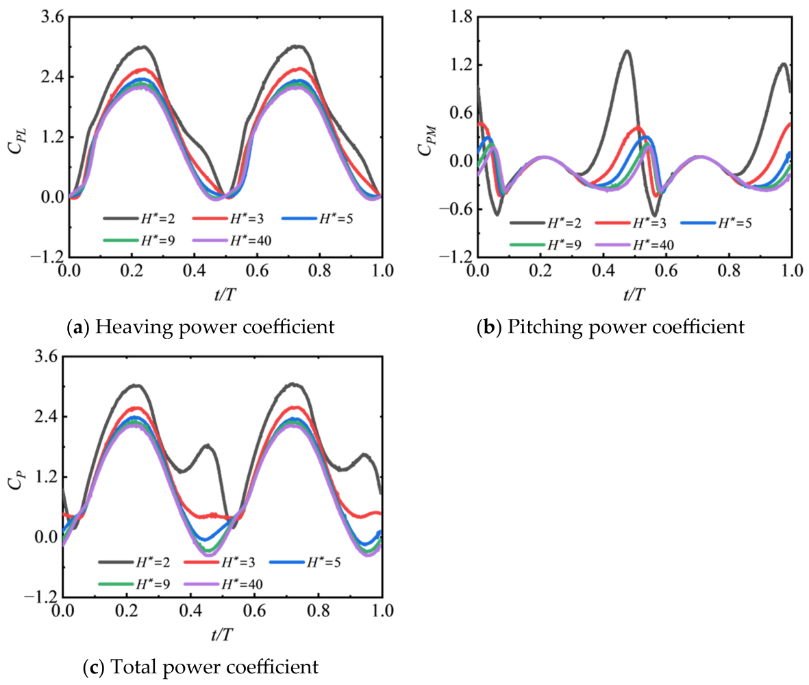
Figure 7 illustrates the variation in power coefficients under different $H^{\ast }$ over one cycle. Combining the lift coefficient in Figure 6a and Equation (10), the instantaneous heaving velocity $\stackrel{·}{h}\left(t\right)=0$ at $t/T=0$ and $t/T=0.5$, leading to $C_{PL}=0$ at these moments. As shown in Figure 6a, the heaving power coefficient ($C_{PL}$) remains almost entirely positive throughout the cycle, with only minor negative fluctuations occurring briefly near $t/T=0$ and $t/T=0.5$. This is because the directions of the lift force and heaving velocity remain consistent for most of the time. The heaving power coefficient reaches a peak near $t/T=0.25$, and the peak value decreases as $H^{\ast }$ increases. This is due to the velocity reaching its maximum value, while the lift force lies in the high lift regime and gradually decreases with increasing $H^{\ast }$. The heaving power coefficient for $H^{\ast }=2$ approaches those of the other cases near $t/T=0.3$, which is because the lift coefficient for $H^{\ast }=2$ is close to that of the other cases at this moment. A significant difference in heaving power coefficients is observed near $t/T=0.45$, since the lift coefficient exhibits a peak here for $H^{\ast }=2$ while remaining stable in the other cases, and the lift coefficient decreases with the increasing $H^{\ast }$.

Figure 7b shows the pitching power coefficient ($C_{PM}$). For $H^{\ast }=2$, the pitching power coefficient first decreases to a negative peak near $t/T=0.05$. It rises to a growth inflection point near $t/T=0.2$. Then, it falls back to a decline inflection point near $t/T=0.3$. Finally, it increases to a positive peak near $t/T=0.5$. According to Equation (11), the pitching power coefficient is closely related to the moment coefficient and pitching angular velocity. The pitching angular velocity $\stackrel{·}{\theta }\left(t\right)$ is positive in the interval $t/T\in \left[0,0.25\right]$ and negative in $t/T\in \left[0.25,0.5\right]$. Therefore, the pitching power coefficient in Figure 7b for $t/T\in \left[0.25,0.5\right]$ is opposite in direction to the moment coefficient in Figure 6b. As $H^{\ast }$ increases, the peak value of the pitching power coefficient decreases and the phase shifts.

A comparison of Figure 7a,c, reveals that the heaving component dominates the total energy harvesting power across all cases. For $H^{\ast }=2$, the pitching power coefficient in Figure 7b exhibits a pronounced peak near $t/T=0.45$, which significantly increases the proportion of pitching power in the total harvesting energy. This leads to a corresponding peak in the total power coefficient ($C_P$) in Figure 7c at the same phase. For $H^{\ast }=3$ within $t/T\in \left[0.4,0.5\right]$, the decrease in the heaving power coefficient is approximately balanced by the increase in the pitching power coefficient, resulting in a stable positive value of the total power coefficient during this interval. In contrast, for $H^{\ast }\ge 5$ in the same interval, the heaving power coefficient is minimized and even becomes negative due to phase shift effect, while the pitching power coefficient also remains negative. Consequently, the total power coefficient decreases with the increasing $H^{\ast }$. These observations collectively demonstrate the influence mechanism of the WIG effect on the energy harvesting performance of the oscillating hydrofoil.

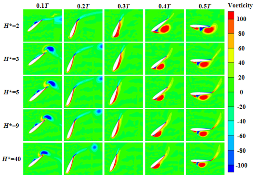
The vorticity contour plots at five equally spaced points in the first half of the motion cycle under typical cases are shown in Figure 8. For $H^{\ast }=2$, when $t/T=0.1$ the leading-edge vortex (LEV) detaches. This causes a significant pressure difference between the upper and lower surfaces of the hydrofoil, and the lift coefficient reaches its peak. The detached vortex reduces the pressure difference between the leading and trailing edges, leading to a decrease in the absolute value of the moment coefficient. Su et al. [2] and Wu et al. [25] also revealed that the proximity of the confining wall reshapes the pressure distribution and amplifies the hydrodynamic loads acting on oscillating hydrofoils. When $t/T=0.2$, the LEV is fully detached, the angle of attack is in a relatively large range. The lift coefficient remains large and stable, and the moment coefficient increases. When $t/T=0.3$, a new LEV forms on the lower surface of the hydrofoil. This vortex reduces the pressure difference between the upper and lower surfaces and decreases the absolute value of the lift coefficient. The deformation of the LEV alters the pressure distribution on the hydrofoil surface, and the moment coefficient reaches a larger value. When $t/T=0.4$, the detachment of the LEV increases the absolute value of the lift coefficient. And its movement toward the trailing edge further increases the absolute value of the moment coefficient. When $t/T=0.5$, the LEV reattaches to the hydrofoil surface, reducing the absolute value of the lift coefficient. While the maximum pressure difference at the trailing edge causes the moment coefficient to reach its peak. The detachment and reattachment of the LEV is responsible for the occurrence of the inflection point in the lift coefficient at $t/T\in \left[0.35,0.5\right]$ under this operating condition. For $H^{\ast }=3$, when $t/T=0.1$, the LEV begins to detach, with the lift coefficient reaching its peak and the moment coefficient showing an inflection point. When $t/T=0.2$, the LEV is fully detached. When $t/T=0.3$, dynamic stall occurs at the leading edge of the oscillating hydrofoil, and the LEV starts to form. This phenomenon leads to the emergence of inflection points in both the lift coefficient and the moment coefficient. At $t/T=0.4$ and $t/T=0.5$, the rearward movement of the LEV increases the absolute value of the moment coefficient. The LEV is in a critical state of shedding and attachment, resulting in almost no change in the lift coefficient during this phase. The development of the remaining cases is similar to that of $H^{\ast }=3$. Notably, as $H^{\ast }$ increases, the timing of vortex generation and detachment is delayed. The phenomenon was also documented in the dynamic stall characterization reported by Ribeiro et al. [9]. This delay leads to a gradual phase shift in the lift and moment coefficients. The variation is attributed to the enhanced WIG effect resulting from the reduced distance between the oscillating hydrofoil and the wall.

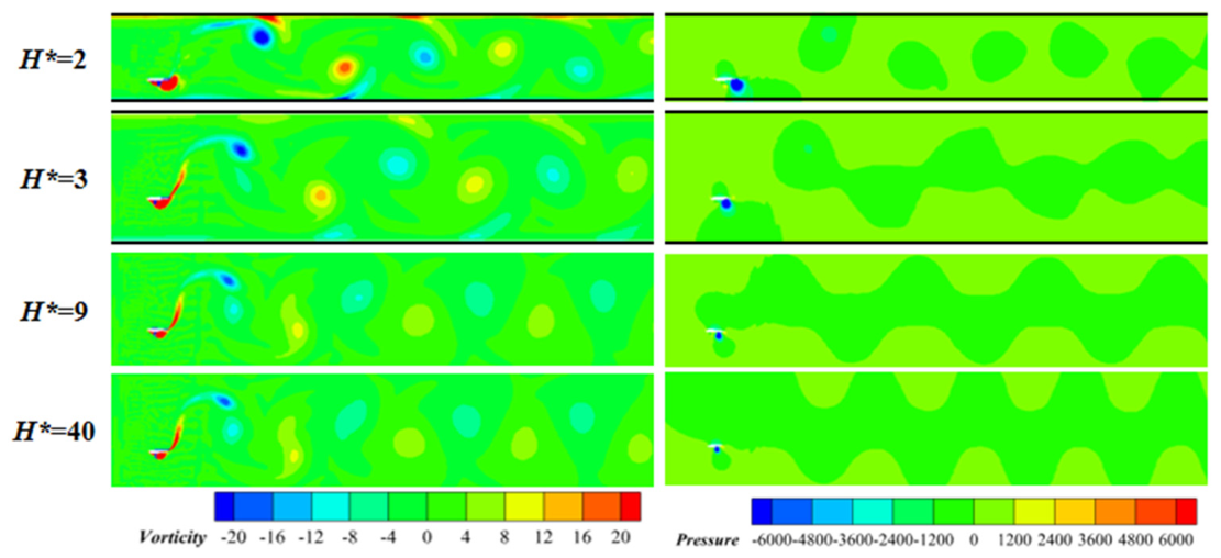
The vorticity and pressure contours of the oscillating hydrofoil wake under $H^{\ast }$ = 2, 3, 9, 40 are shown in Figure 9. At $H^{\ast }=2$, the upper and lower walls strongly restrict the transverse development of the wake and intensify the interactions among the shear layers, the shed vortices, and the confining walls. Consequently, compact regions of positive and negative vorticity appear in the near wake, while the corresponding pressure disturbances remain relatively localized within the narrow channel. When $H^{\ast }$ increases to 3, the wake is allowed to expand further in the transverse direction. The initially compact vortical structures evolve into a broader staggered pattern, accompanied by a more continuous downstream undulation of the pressure field.

This wall-induced modification of the wake is qualitatively consistent with the observations reported by He et al. [23], who showed that the proximity of a solid boundary can alter vortex formation, pressure distribution, and wake development. In particular, Mo et al. [28] attributed the single-wall pressure enhancement to the positive-pressure region generated on the wall-facing surface as the flow is partially blocked within the foil–wall gap. The present results exhibit a similar confinement-induced mechanism; however, the bilateral configuration considered here introduces simultaneous interactions with both the upper and lower walls. This enables the combined effects of wall spacing, symmetric confinement, and wake–wall coupling to be quantified, and, further, allows a critical wall distance to be identified over a range of Reynolds numbers and oscillation frequencies.

As $H^{\ast }$ further increases, the wall-induced modification of the wake progressively weakens. In particular, the vortex arrangement, transverse wake extent, vortex spacing, and downstream pressure distribution at $H^{\ast }=9$ are already close to those observed at the far-wall reference condition of $H^{\ast }=40$. This similarity provides flow field evidence supporting the efficiency-based result that the bilateral WIG effect becomes weak at approximately $H^{\ast }=9$. The apparent attenuation of the downstream vortical structures does not materially affect this conclusion. It should be emphasized that the apparent attenuation of the downstream vorticity may also be affected by wake-grid resolution, turbulent diffusion inherent in the URANS formulation, and numerical dissipation. Therefore, the present comparison focuses on the relative differences in the near-wake organization rather than on the quantitative decay rate of the far-wake vortices.

4.2. The Influence of the Oscillation Frequency on Energy Harvesting Efficiency

Based on the aforementioned findings, the hydrodynamic characteristics of the oscillating hydrofoil can be considered unaffected by the WIG effect when dimensionless wall distance $H^{\ast }\ge 9$. To investigate the influence of the oscillation frequency on the energy harvesting performance of the oscillating hydrofoil, the dimensionless oscillation frequency $f^{*}$ is varied under the condition of $H^{\ast }=9$ with other parameters fixed. According to the review by Liu et al. [22] concerning the correlation between peak energy harvesting efficiency and oscillation frequency, the range of $f^{*}$ is set as $f^{*}\in [0.06,0.24]$. Meanwhile, to reveal the correlation mechanism of the oscillation frequency and the WIG effect on energy harvesting performance of the oscillating hydrofoil, the case of $H^{\ast }=40$, where the WIG effect is completely negligible, is set as the control group.

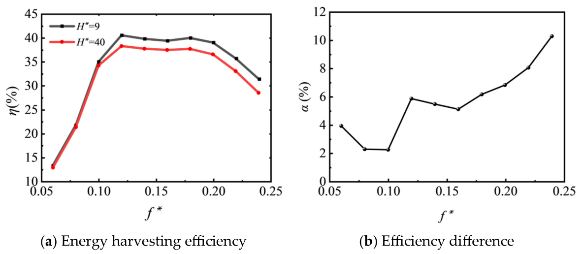
Figure 10 presents the energy harvesting efficiency under different $f^{*}$ values, and the difference in energy harvesting efficiency between the conditions of $H^{\ast }=9$ and $H^{\ast }=40$. As shown in Figure 10a, when $f^{*}\le 0.12$, the energy harvesting efficiency of the oscillating hydrofoil increases rapidly with the increase of $f^{*}$, and reaches its maximum at $f^{*}=0.12$. The peak energy harvesting efficiencies under the $H^{\ast }=9$ and $H^{\ast }=40$ conditions are 40.5% and 38.3%, respectively. Subsequently, the energy harvesting efficiency decreases slowly with the increase of $f^{*}$, while a minor secondary peak appears near $f^{*}=0.18$. When $f^{*}\ge 0.2$, the energy harvesting efficiency decreases rapidly as $f^{*}$ increases. As illustrated in Figure 10b, the difference in energy harvesting efficiency between $H^{\ast }=9$ and $H^{\ast }=40$ is insignificant when $f^{*}\le 0.1$, reaches a local peak at $f^{*}=0.12$, and then decreases slightly. When $f^{*}\ge 0.16$, the WIG effect on the oscillating hydrofoil becomes increasingly prominent with increasing $f^{*}$, exhibiting an overall higher sensitivity to the oscillation frequency. Wang et al. [26] and Zhu et al. [27] also noted that the favorable effects induced by the WIG effect become more pronounced with increasing oscillation frequency.

Five typical cases under the $H^{\ast }=9$ condition with $f^{*}$ = 0.06, 0.12, 0.14, 0.18, 0.24 are selected for further analysis. Among them, the case at $f^{*}=0.14$ is consistent with the $H^{\ast }=9$ condition in the previous section, and is therefore selected as the baseline case for this research.

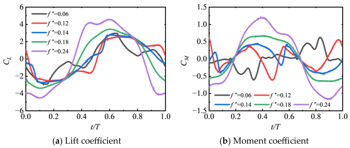
Figure 11 shows the lift coefficient and moment coefficient curves of the oscillating hydrofoil under different $f^{*}$ conditions. Compared with the baseline case, the lift coefficient under $f^{*}=0.12$ exhibits a significant difference in the interval $t/T\in \left[0.3,0.5\right]$, with two peak inflection points appearing near $t/T=0.35$ and $t/T=0.46$. For the $f^{*}=0.06$ case, the lift coefficient rises rapidly after reaching a peak near $t/T=0.16$, with inflection points occurring near $t/T=0.3$ and $t/T=0.42$, respectively. Under the $f^{*}=0.18$ condition, the lift coefficient first decreases, reaches a peak near $t/T=0.1$, and then increases steadily without a plateau stage. For the $f^{*}=0.24$ case, the lift coefficient reaches a peak near $t/T=0.1$, then increases gradually at first and then rapidly to another peak near $t/T=0.45$, followed by an inflection point near $t/T=0.5$. The comparison shows that as $f^{*}$ increases, the peak value of the lift coefficient gradually increases with a slight phase advance.

Figure 11b presents the moment coefficient curves. The moment coefficient under $f^{*}=0.12$ shows an obvious phase advance compared with the baseline case. It starts with a large initial value and decreases rapidly, rebounding after an inflection point near $t/T=0.07$. Then, it decreases immediately after another inflection point near $t/T=0.3$, and reaches its peak near $t/T=0.5$. The variation in the moment coefficient under $f^{*}=0.06$ is significantly different from that of other cases. In the first half of the cycle, the moment coefficient only fluctuates greatly in the interval $t/T\in \left[0.2,0.4\right]$, with inflection points near $t/T=0.25$ and $t/T=0.3$, and reaches its peak near $t/T=0.35$, while $C_M\approx 0$ at other times. For the $f^{*}=0.18$ case, the moment coefficient first increases to near $t/T=0.3$ and then rises gently, reaching its peak near $t/T=0.4$ before decreasing slowly. Under the $f^{*}=0.24$ condition, the moment coefficient starts to increase near $t/T=0.1$, reaches its peak near $t/T=0.4$, and then decreases rapidly.

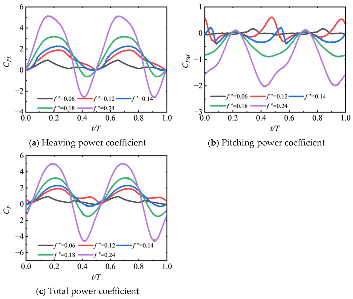
The power coefficients under different $f^{*}$ conditions are shown in Figure 12. As indicated in Figure 12a, the heaving power coefficient is positive for most of the cycle under $f^{*}=0.12$, exhibiting a trend of first increasing and then decreasing. It reaches its peak near $t/T=0.25$, where the lift coefficient and the heaving velocity are in the same direction and both attain relatively large values. The $f^{*}=0.06$ case shows distinct differences from the other cases. Its heaving power coefficient peaks near $t/T=0.16$, which also corresponds to the maximum value of the lift coefficient, and then gradually decreases as the lift coefficient drops rapidly. Compared with the baseline case, the heaving power coefficients under $f^{*}=0.18$ and $f^{*}=0.24$ exhibit an additional obvious negative region. This occurs because the lift coefficient reverses direction in advance within $t/T\in \left[0.35,0.4\right]$, leading to an opposite sign relative to the heaving velocity. The comparison of the heaving power coefficients for $f^{*}\in [0.12,0.24]$ reveals that as $f^{*}$ increases, the peak of the heaving power coefficient appears earlier and its magnitude increases.

As shown in Figure 12b, the pitch power coefficient under $f^{*}=0.12$ shows a similar trend to the baseline case. Compared with the baseline case, its positive pitch power coefficient interval is expanded. The positive peak is significantly advanced and increased in magnitude, while the negative peak is slightly reduced. This is related to the variations in the peak value and phase of the moment coefficient in Figure 11b. For the $f^{*}=0.06$ case, due to the small moment coefficient, a small pitch power coefficient only exists in the interval $t/T\in \left[0.3,0.4\right]$, while the pitch angular velocity is small in $t/T\in \left[0.2,0.3\right]$, resulting in a low power coefficient. Under $f^{*}=0.18$ and $f^{*}=0.24$, the pitch power coefficient is negative for most of the cycle and only positive in $t/T\in \left[0.18,0.25\right]$. The moment coefficient crosses zero near $f^{*}=0.18$ and then becomes in phase with the pitch angular velocity, until they become out of phase again at $t/T=0.25$ as the pitch angular velocity reverses direction. The comparison for $f^{*}\in [0.12,0.24]$ shows that as $f^{*}$ increases, the peak value of the moment coefficient in $t/T\in \left[0.25,0.5\right]$ gradually increases, and the negative peak of the pitch power coefficient increases significantly.

The instantaneous total power coefficients for different $f^{*}$ can be obtained from Figure 12c. The trend and peak of the total power coefficient are highly consistent with those of the heaving power coefficient, indicating that the heaving power dominates the energy harvesting process of the oscillating hydrofoil in most cases. It is worth noting, however, that under $f^{*}=0.12$, the heaving power is small while the pitch power is large in the interval $t/T\in \left[0.4,0.5\right]$, making the pitch power dominant. When $f^{*}\ge 0.14$, the negative pitch power becomes significant, leading to an obvious expansion of the negative power interval. This results in a reduction in energy harvesting efficiency as $f^{*}$ increases.

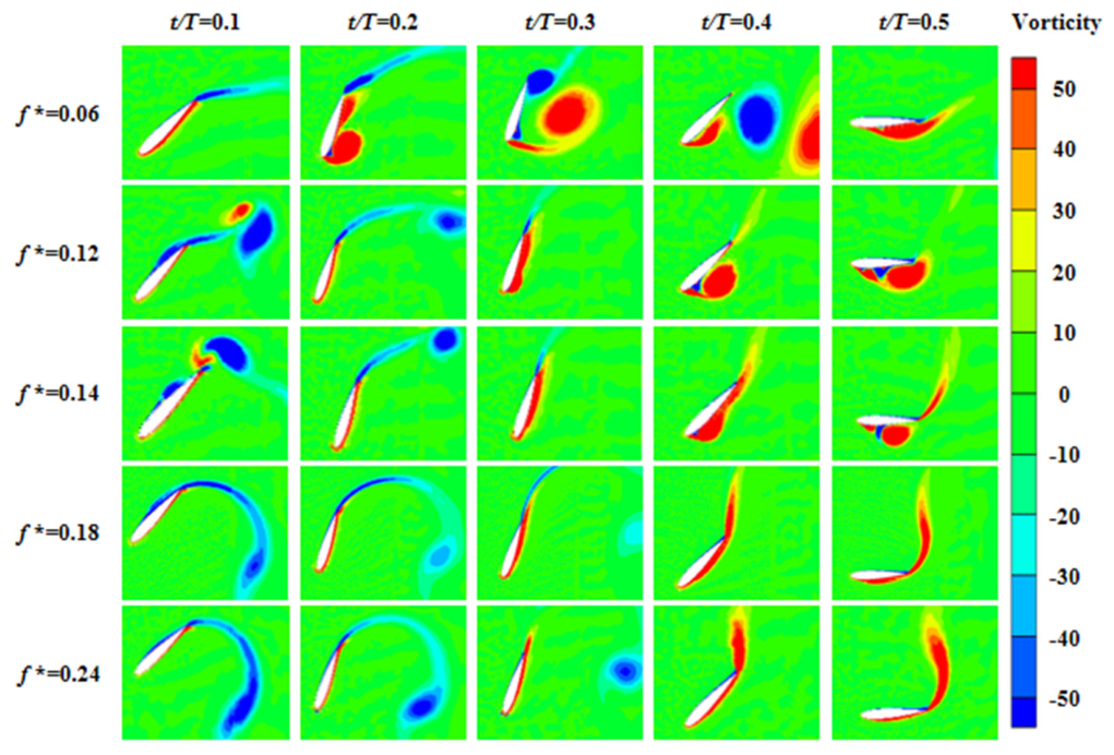
Wang et al. [26] and Zhu et al. [27] reported that higher oscillation frequencies alter the phase relationship between hydrodynamic loads and hydrofoil motion. The present study extends these observations, demonstrating that frequency effects manifest not only in the cycle-averaged energy harvesting efficiency but also in the timings of LEV formation, shedding, and reattachment. The vorticity cloud in Figure 13 illustrates the evolution of the flow field around the oscillating hydrofoil under different $f^{*}$ conditions. The case with $f^{*}=0.14$ is consistent with the $H^{\ast }=9$ condition investigated in Section 4.1, and its vorticity field evolution is not repeated here. For $f^{*}=0.12$, the vortex development is similar to the baseline case, but vortex generation and shedding occur earlier. From $t/T=0.4$ to $t/T=0.5$, the leading-edge vortex (LEV) shifts rearward and enters a critical state between attachment and shedding. This causes the pressure difference between the upper and lower surfaces to first increase slightly and then decrease, with the absolute value of the lift coefficient first increasing slightly and then decreasing rapidly. Meanwhile, the rearward shift of the vortex moves the low-pressure region backward, increasing the pressure difference between the leading and trailing edges and causing the moment coefficient to rise gradually to its peak.

For $f^{*}=0.06$, at $t/T=0.1$, the vortex structures at the trailing edge shed continuously. As the angle of attack increases, the vortex forms on the lower surface, increasing the pressure difference between the upper and lower surfaces and the absolute value of the lift coefficient. The pressure difference between the leading and trailing edges remains small, so $C_M\approx 0$. At $t/T=0.2$, a LEV forms on the lower surface, reducing the upper–lower pressure difference and causing the lift coefficient to decrease rapidly. Meanwhile, the trailing vortex structures increase the leading–trailing pressure difference, driving the moment coefficient to a local peak. From $t/T=0.3$ to $t/T=0.4$, the leading main vortex and trailing vortex shed successively. Under their combined influence, the upper–lower pressure difference increases slightly, leading to a minor rise in the lift coefficient. The leading–trailing pressure difference gradually decreases, causing the moment coefficient to drop. At $t/T=0.5$, the LEV reattaches to the lower surface and moves rearward, with the moment coefficient fluctuating at a low value while the lift coefficient increases.

The vortex dynamic behaviors are similar for $f^{*}=0.18$ and $f^{*}=0.24$; no dynamic stall occurs during the oscillating hydrofoil motion, so no LEV is generated. From $t/T=0.1$ to $t/T=0.2$, the shed trailing vortex moves downward clockwise, reducing the upper–lower pressure difference and causing the lift coefficient to decrease gradually from its peak. The leading–trailing pressure difference also decreases, and the moment coefficient begins to drop. From $t/T=0.3$ to $t/T=0.4$, the trailing vortex continuously detaches upward, reversing the direction of the upper–lower pressure difference. The lift coefficient decreases and then increases in the opposite direction to a peak, while the leading–trailing pressure difference gradually increases, driving the moment coefficient to its peak. At $t/T=0.5$, the trailing vortex curls upward counterclockwise, the lift coefficient increases slowly, and the moment coefficient decreases gradually before maintaining a relatively high value.

4.3. The Influence of the Reynolds Number on Energy Harvesting Efficiency

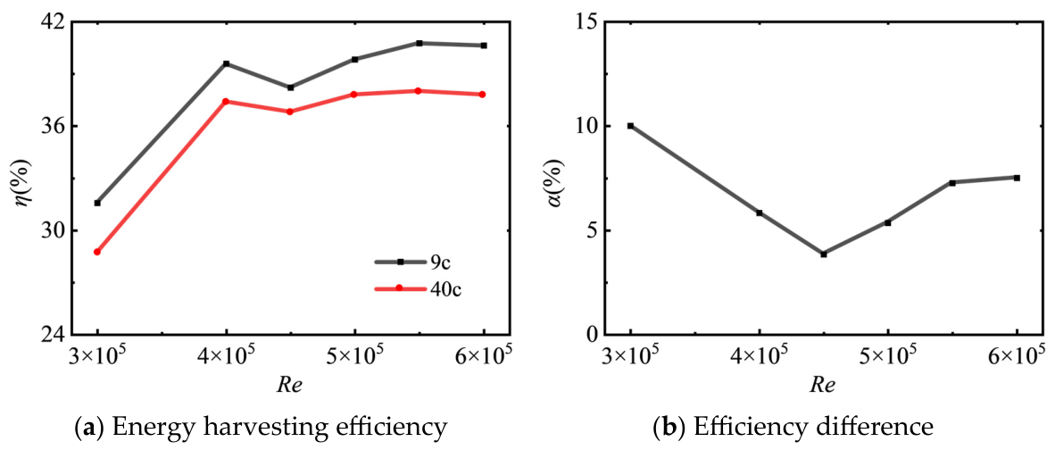
To investigate the correlation mechanism of the Reynolds number ($Re$) and the WIG effect on the energy harvesting efficiency of the oscillating hydrofoil, $Re$ is varied under the condition $H^{\ast }=9$. The results are compared with those obtained at $H^{\ast }=40$ where the WIG effect is negligible. The range of $Re$ considered in this research is $[3\times {10}^5,6\times {10}^5]$. Figure 14 presents the energy harvesting efficiency curves at different $Re$ and the difference curves of energy harvesting efficiency between the $H^{\ast }=9$ and $H^{\ast }=40$ conditions. As shown in Figure 14a, the energy harvesting efficiency exhibits the double-peak characteristic with varying $Re$, with two peaks occurring at $Re=4\times {10}^5$ and $Re=5.5\times {10}^5$. Although the absolute energy harvesting efficiency generally increases with $Re$ [6,7,8,9,10], the relative WIG influence varies non-monotonically, decreasing first and then increasing as $Re$ rises. As shown in Figure 14b, the efficiency difference decreases rapidly with the increasing $Re$ in the range $Re\in [3\times {10}^5,4.5\times {10}^5]$. This is because the difference in energy harvesting efficiency remains nearly constant while the efficiency itself increases rapidly, leading to a decrease in its ratio. In the range $Re\in [4.5\times {10}^5,6\times {10}^5]$, the efficiency difference gradually increases with the increasing $Re$, indicating that the influence of the WIG effect on the hydrofoil’s energy harvesting performance becomes increasingly prominent. Six typical cases under the $H^{\ast }=9$ condition, including $Re=3\times {10}^5$, $4\times {10}^5$, $4.5\times {10}^5$, $5\times {10}^5$, $5.5\times {10}^5$, and $6\times {10}^5$, are selected for analysis. Among these, the case at $Re=5\times {10}^5$ corresponds to the $H^{\ast }=9$ condition investigated in Section 4.1, and is therefore selected as the baseline case for this section.

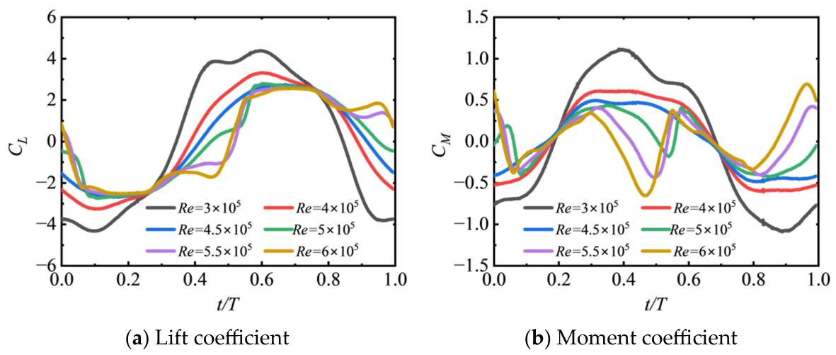
Figure 15 presents the lift and moment coefficients of the oscillating hydrofoil under different $Re$ conditions. As shown in Figure 15a, for $Re\in [3\times {10}^5,4.5\times {10}^5]$, the lift coefficient rises rapidly after reaching a peak near $t/T=0.1$, and its variation is smooth without obvious inflection points before the peak compared with the baseline case. Under $Re=5.5\times {10}^5$ and $Re=6\times {10}^5$, the lift coefficient follows a trend similar to the baseline case but with earlier inflection points. The comparison shows that the peak lift coefficient tends to decrease as $Re$ increases.

The moment coefficient curves are shown in Figure 15b. The moment coefficients exhibit similar trends for $Re\in [3\times {10}^5,4.5\times {10}^5]$. Compared with $Re=4\times {10}^5$ and $Re=4.5\times {10}^5$, where the moment coefficient changes smoothly after peaking near $t/T=0.3$, the case at $Re=3\times {10}^5$ shows a rapid decrease after the moment coefficient peaks in $t/T\in \left[0.4,0.5\right]$. The moment coefficients also show similar trends for $Re\in [5\times {10}^5,6\times {10}^5]$. As $Re$ increases, the peak moment coefficient increases with an obvious phase advance.

A comparison between Figure 15 and Figure 11 shows that the lift coefficient trends for $Re=3\times {10}^5$, $Re=4\times {10}^5$, and $Re=6\times {10}^5$ in this section are highly similar to those for $f^{*}=0.24$, $f^{*}=0.18$, and $f^{*}=0.12$ in Section 4.2. Since the oscillation frequency is the same for all Reynolds number cases in this section, calculation verifies that the dimensionless frequencies corresponding to $Re=3\times {10}^5$, $Re=4\times {10}^5$, and $Re=6\times {10}^5$ are close to those of $f^{*}=0.24$, $f^{*}=0.18$, and $f^{*}=0.12$ in Section 4.2. The effective angles of attack are basically the same, and the force characteristics of the hydrofoil under dynamic stall are also highly consistent.

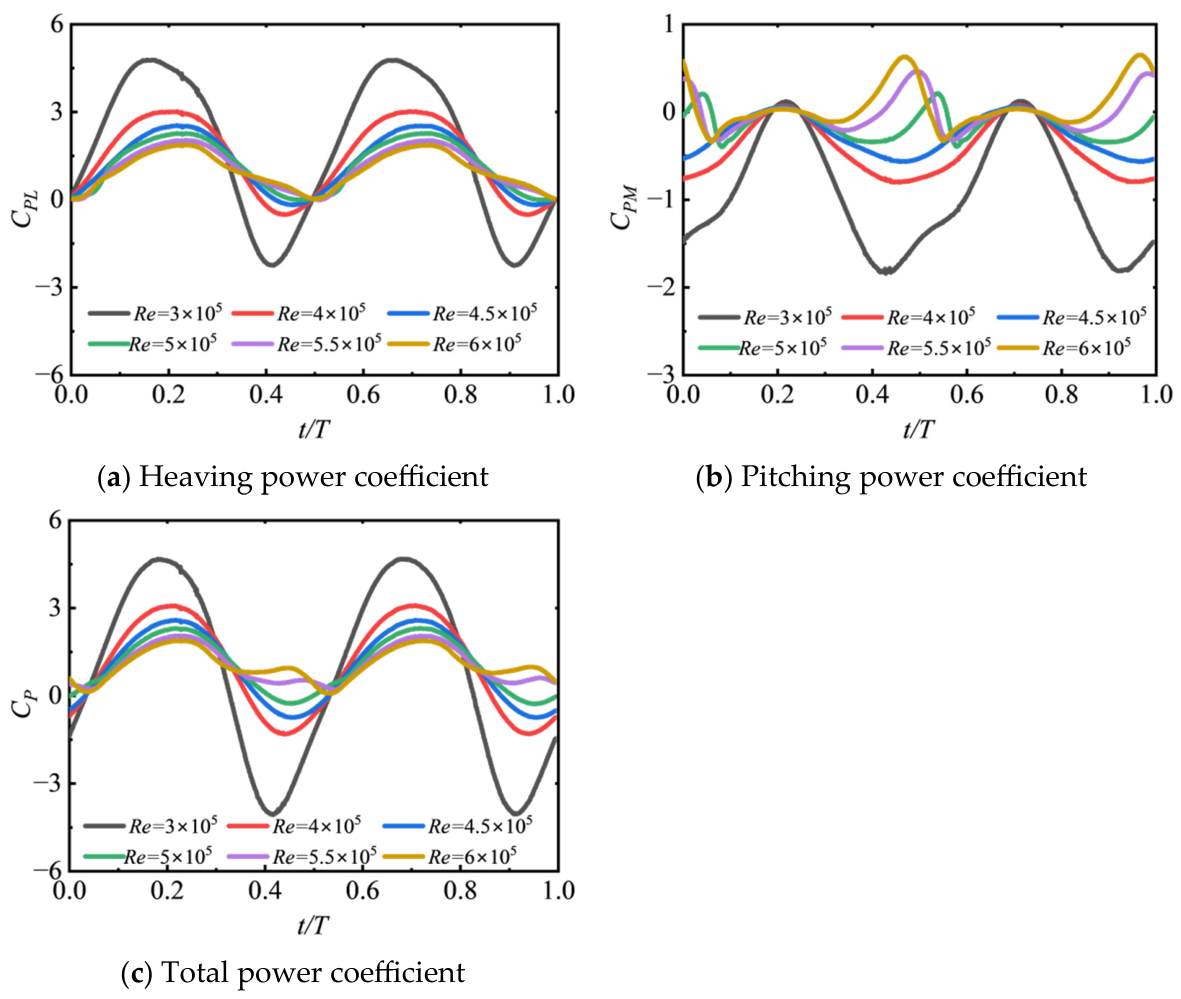
Figure 16 presents the power coefficients under different $Re$ conditions. As indicated in Figure 16a, for $Re\in [3\times {10}^5,4.5\times {10}^5]$, the heaving power coefficient exhibits a similar trend of increasing, then decreasing, and then increasing again in the first half of the cycle. The negative region of the heaving power coefficient is caused by the lift coefficient and heaving velocity being in opposite directions. For $Re\in [5\times {10}^5,6\times {10}^5]$, the heaving power coefficient shows a trend of first increasing then decreasing, and remains positive throughout the entire cycle. This is because the lift coefficient and heaving velocity are always in the same direction. A comparison of all cases shows that the peak heaving power coefficient gradually decreases with increasing $Re$.

Figure 16b presents the pitching power coefficient curves. For $Re\in [3\times {10}^5,4.5\times {10}^5]$, the pitching power coefficient first increases and then decreases. The amplitude of the negative power decreases and the phase shifts rearward as $Re$ increases. The positive pitching power coefficient appears near $t/T=0.2$, corresponding to the moment coefficient crossing zero at that moment and becoming in phase with the pitching angular velocity. They become out of phase again at $t/T=0.25$ when the pitching angular velocity reverses direction. The pitching power coefficient for $Re\in [5\times {10}^5,6\times {10}^5]$ shows similar variations. As Re increases, the peak of the pitching power coefficient appears progressively earlier with a larger amplitude.

The total power coefficient follows the same trend as the heaving power coefficient for most of the cycle according to Figure 16c. However, in the interval $t/T\in \left[0.4,0.5\right]$, the pitching power coefficient reaches its peak while the heaving power coefficient gradually decreases, making the pitching power coefficient dominant in the total power coefficient. Under $Re=3\times {10}^5$, the negative power coefficient region expands significantly, corresponding to the minimum energy harvesting efficiency at this condition. For $Re\in [5.5\times {10}^5,6\times {10}^5]$, a positive inflection point appears in the total power coefficient near $t/T=0.45$. Compared with other cases, the negative region is greatly reduced, corresponding to an increase in the energy harvesting efficiency.

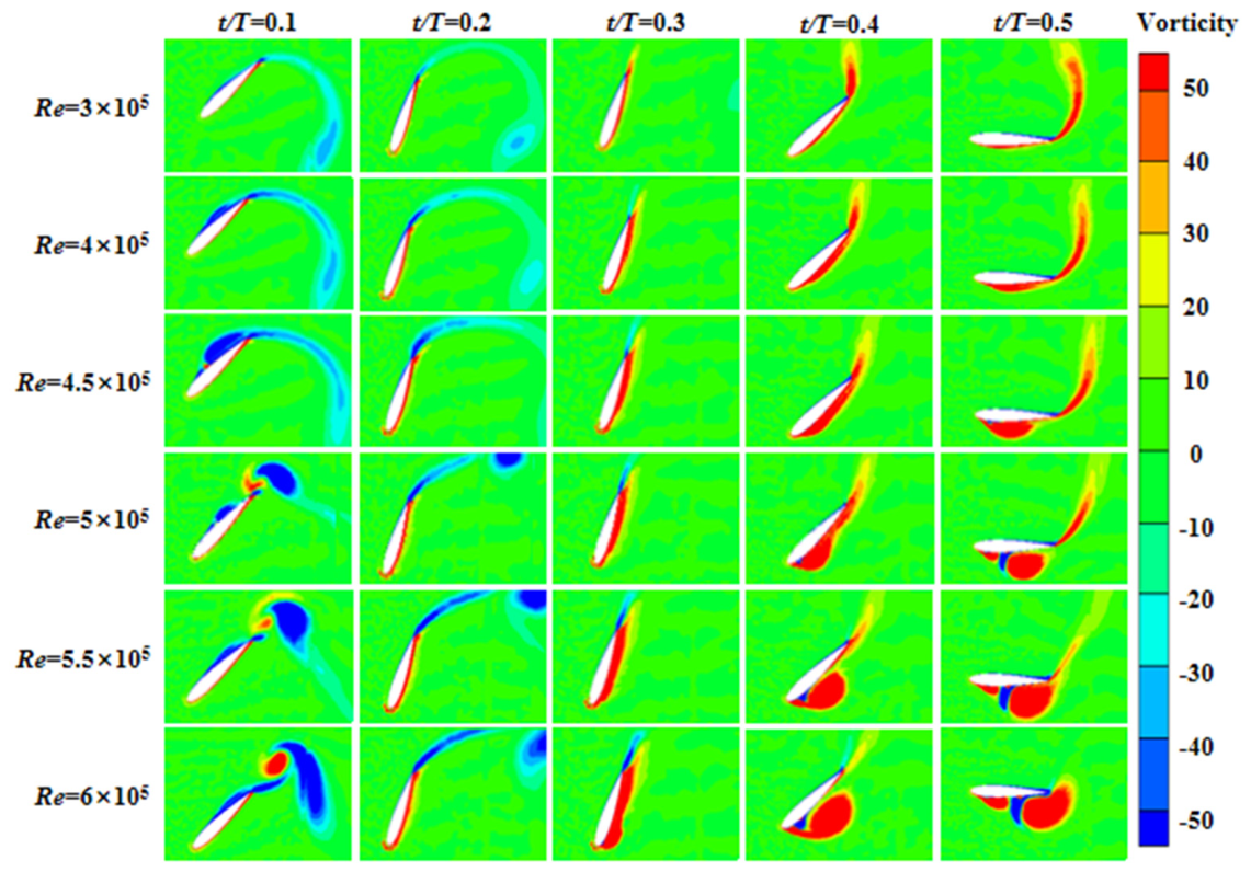
Ribeiro et al. [9] observed the effects of $Re$ on the formation and shedding of LEV. Figure 17 shows the vorticity cloud illustrating the evolution of the flow field around the oscillating hydrofoil under different $Re$ conditions.

For $Re=3\times {10}^5$, no dynamic stall occurs during the hydrofoil motion, and thus no LEV is generated. The surface pressure distribution is mainly governed by the variation in the effective angle of attack. As $Re$ increases, vortices gradually appear on both upper and lower surfaces of the hydrofoil at $Re=4\times {10}^5$ and $Re=4.5\times {10}^5$. From $t/T=0.1$ to $t/T=0.2$, the LEV shifts rearward and gradually sheds. The lift coefficient decreases slowly from its peak. The pressure difference between the leading and trailing edges reduces, leading to a gradual decrease in the moment coefficient. At $t/T=0.3$, the LEV begins to form. The pressure difference between the upper and lower surfaces decreases, and the lift coefficient starts to drop. The moment coefficient reaches its peak and then remains stable. From $t/T=0.4$ to $t/T=0.5$, the LEV shifts rearward. The pressure difference between the upper and lower surfaces increases, and the lift coefficient rises gradually. The vortex distribution on the lower surface remains uniform, so the moment coefficient stays stable. For $Re\in [5\times {10}^5,6\times {10}^5]$, the vortex dynamics show similar characteristics. The key moments of vortex formation and evolution shift slightly earlier as $Re$ increases. From $t/T=0.1$ to $t/T=0.2$, the LEV sheds and the pressure difference between the upper and lower surfaces is large. The lift coefficient reaches its peak and then remains stable. The gradual increase in the effective angle of attack reduces the pressure difference between the leading and trailing edges, causing the moment coefficient to decrease. At $t/T=0.3$, dynamic stall occurs at the hydrofoil leading edge. The LEV begins to form, and inflection points appear in both the lift and moment coefficients. From $t/T=0.4$ to $t/T=0.5$, the LEV shifts rearward. As $Re$ increases, a shedding and reattachment phenomenon of the LEV gradually emerges.

4.4. The Coupled Effect of $Re$, Oscillation Frequency $f$ and $H^{\ast }$, and GMM-Based Prediction of the Critical Wall Distance

Based on the single parameter analysis, this section further explores the coupled effect of $Re$, the oscillation frequency $f$ and $H^{\ast }$ to provide a quantitative basis for parameter selection to avoid the WIG effect in the oscillating hydrofoil experiment. To efficiently and uniformly cover the parameter space, the orthogonal experimental design is adopted for sampling. During the sampling process, the hydrofoil geometry, wall properties, numerical settings, and all other geometric and kinematic parameters are kept constant, whereas $Re$, $f$, and $H^{\ast }$ are varied within their prescribed ranges.

Unlike Section 4.1, Section 4.2 and Section 4.3, which are conducted at the relatively higher-Reynolds-number regime, the present section extends the sampling range to $Re\in [1\times {10}^3,6\times {10}^5]$ to construct the coupled $Re$-$f$-$H^{\ast }$ dataset. Accordingly, the flow model is selected based on the Reynolds number regime. For the cases at $Re=1\times {10}^3$, the laminar formulation is employed without an additional turbulence closure, consistent with the lower-Reynolds-number numerical treatment [8].

To assess the reliability of the numerical treatment near $Re=1\times {10}^3$, an additional benchmark calculation is performed using the oscillating hydrofoil configuration reported by Kinsey and Dumas [8]. The comparison is conducted using the same geometric and kinematic parameters as those in the reference study, with $Re=1.1\times {10}^3$ and $f^{*}=0.14$. As summarized in

Table 4. Low-Reynolds number validation against the numerical results reported by Kinsey and Dumas [8].

Quantity	Present Study	Reference	Relative Difference (%)
${C_L}_{\max }$	1.889	1.942	2.7
$\overline{C_P}$	0.840	0.860	2.3
$\eta$ (%)	32.9	33.7	2.4

, the predicted maximum lift coefficient, cycle-averaged power coefficient, and energy harvesting efficiency are 1.889, 0.840, and 32.9%, respectively. The corresponding relative differences from the reference values are 2.7%, 2.3%, and 2.4%, respectively. The close agreement indicates that the present laminar numerical formulation provides reliable predictions of the principal integrated hydrodynamic and energy harvesting quantities near $Re=1\times {10}^3$.

For all remaining sampled cases with $Re\ge 5\times {10}^4$, the SA model is adopted. To assess the sensitivity of the numerical results to the model selection, an additional comparison is performed at $Re=5\times {10}^4$ using both the laminar and SA models under otherwise identical numerical conditions.

As shown in

Table 5. Comparison of the laminar and SA models at $Re=5\times {10}^4$.

Quantity	Laminar	SA	Relative Difference (%)
${C_L}_{\max }$	1.640	1.590	3.1
$\overline{C_P}$	0.861	0.839	2.5

, the laminar and SA models predict similar maximum lift coefficients and cycle-averaged power coefficients at $Re=5\times {10}^4$, with relative differences of 3.1% and 2.5%, respectively. These results indicate that the selected hydrodynamic and energy harvesting quantities exhibit only limited sensitivity to the flow formulation at this Reynolds number. Therefore, the Laminar model is used for the sampled cases at $Re=1\times {10}^3$, whereas the SA model is used for the remaining sampled cases at $Re\ge 5\times {10}^4$. This numerical distinction is specific to the discrete Reynolds number levels, hydrofoil configuration, and prescribed motion considered in the present study and should not be interpreted as identifying a universal laminar-to-turbulent transition Reynolds number.

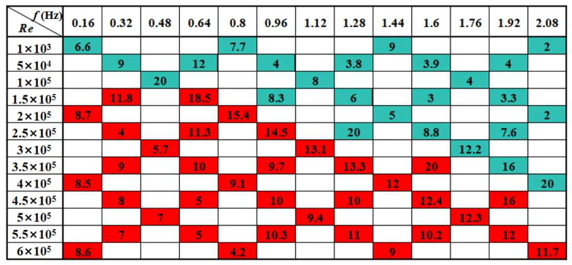
The investigated ranges of the Reynolds number and oscillation frequency are determined based on the preceding parametric analysis, where $Re\in [1\times {10}^3,6\times {10}^5]$ and $f\in [0.16,2.08]$ are selected to represent the effective operating conditions for evaluating the coupled influence of these parameters on the bilateral WIG effect. Numerical simulations are conducted for each sampling condition under different parameters. The critical $H^{\ast }$ for negligible WIG effect is obtained when the deviation of the energy harvesting efficiency between the given condition and the reference condition is below the 5% threshold.

As reported by Kinsey and Dumas [8], the oscillating hydrofoil is classified into propulsion mode and energy harvesting mode, which are governed by the oscillation frequency and the free-stream velocity. In Figure 18, cyan squares correspond to the propulsion mode, while red squares correspond to the energy harvesting mode. It can be seen that the relationships among $H^{\ast }$, $Re$ and $f$ are not simply linear under all conditions. Therefore, nonlinear surface fitting models are employed to fit the critical $H^{\ast }$ under different $Re$ and $f$ combinations, providing quantitative support for parameter selection considering the WIG effect in experiments.

Gaussian mixture models (GMM) provide a probabilistic representation of multimodal and nonlinear datasets and have been widely used for density estimation, clustering, and conditional regression [33,34]. In the present study, GMM-based regression is adopted to establish a finite-component probabilistic representation of the joint relationship among the Reynolds number, oscillation frequency, and critical wall distance. Based on the calibrated mixture model, the conditional distribution of the critical wall distance can be evaluated directly under different flow conditions. The model is represented by a finite set of mixture weights, mean vectors, and covariance matrices, enabling local variations within the investigated parameter space to be captured while maintaining a compact probabilistic formulation. Such a representation is well aligned with the objective of the present study; namely, preliminary parameter mapping of the critical wall distance under different operating conditions.

The 61 numerical samples are divided into a calibration set containing 49 samples and a hold-out validation set containing 12 samples. The validation samples are selected using a space-covering strategy in the normalized $Re$-$f$ parameter space so that they represent the investigated domain rather than being concentrated in a limited local region. Repeated five-fold cross-validation is performed exclusively within the calibration set for model comparison and model selection. The hold-out samples are not used during model selection and are subsequently employed only to evaluate the generalization performance of the selected model.

The root mean square error ($RMSE$) and R-square ($R^2$) are used as evaluation metrics. The mathematical expression of $RMSE$ is

$$RMSE={\left[{\displaystyle \frac{1}{n}}{\displaystyle \sum _{i=1}^n{\left(y_i-y_{ic}\right)}^2}\right]}^{{\displaystyle \frac{1}{2}}},$$

(20)

where $n$ is the total number of samples, $y_i$ is the $H^{\ast }$ result obtained from numerical simulation, and $y_{ic}$ is the predicted value from the model under the same condition. The magnitude of $RMSE$ directly reflects the accuracy of model fitting. The mathematical expression of $R^2$ is

$$R^2=1-{\displaystyle \frac{{\displaystyle {\sum }_{i=1}^n{\left(y_i-y_{ic}\right)}^2}}{{\sigma }^2}},$$

(21)

where $\sigma$ is the standard deviation of $H^{\ast }$. The value of $R^2\to 1$ indicates a better fit between the model and the actual data. After model selection, models are evaluated using the 12 untouched hold-out validation samples. The key indicators of different models are compared in

Table 6. Predictive performance of the candidate regression models.

Model	Repeated Five-Fold CV $\mathit{R}\mathit{M}\mathit{S}\mathit{E}$	Repeated Five-Fold CV ${\mathit{R}}^2$	Hold-Out $\mathit{R}\mathit{M}\mathit{S}\mathit{E}$	Hold-Out ${\mathit{R}}^2$
Normalized polynomial model	$5.015\pm 0.835$	$0.046\pm 0.351$	2.903	0.292
Two-component GMM	$4.386\pm 0.555$	$0.272\pm 0.212$	2.864	0.311
Four-component GMM	$3.293\pm 1.281$	$0.577\pm 0.272$	1.991	0.667
Six-component GMM	$4.235\pm 1.227$	$0.273\pm 0.487$	2.594	0.435

.

As shown in Table 6, the four-component GMM achieves the lowest mean repeated cross-validation $RMSE=3.293\pm 1.281$ and the highest mean cross-validation $R^2=0.577\pm 0.272$ among the candidate models. Based solely on these cross-validation results, the four-component GMM is selected as the final model. When subsequently evaluated using the 12-sample hold-out set, it achieves an $RMSE$ of 1.991 and an $R^2$ of 0.667. The polynomial model is difficult to capture the nonlinear coupling between $H^{\ast }$ and the other parameters and exhibit low fitting accuracy. The two-component GMM has limited capability to describe strong nonlinear variations in higher-Reynolds-number regions due to insufficient components. Increasing the number of components from four to six does not improve the cross-validation performance and results in greater variability among the validation folds, suggesting increased model variance and a potential tendency toward overfitting. Considering both accuracy and stability, the four-component Gaussian mixture model is selected as the optimal fitting model. Nevertheless, the relatively large variation in the cross-validation scores indicates that the model should be interpreted as a preliminary predictor rather than a high-precision universal model.

The critical wall distance is determined from discretely sampled wall distances using a prescribed 5% efficiency-deviation threshold. Consequently, the resulting response may exhibit local stepwise variations or transition-like behavior rather than forming a globally smooth surface. The four Gaussian components are therefore treated as latent statistical components that provide a flexible local approximation of the joint distribution, rather than as four distinct physical flow regimes.

To eliminate the interference of the numerical magnitude differences of different independent variables on the fitting results, the normalized variables $R{e}^{*}$ and $\widehat{f}$ are defined for the independent variables $Re$ and $f$, respectively:

$$R{e}^{*}=\left(Re-{\mu }_{Re}\right)/{\sigma }_{Re},$$

(22)

$$\widehat{f}=\left(f-{\mu }_f\right)/{\sigma }_f,$$

(23)

where ${\mu }_{Re}=302566.6667$ and ${\mu }_f=1.1173$ are the sample means and ${\sigma }_{Re}=187069.6749$ and ${\sigma }_f=0.6019$ are the sample standard deviations of $Re$ and $f$, respectively.

The four-component GMM effectively captures the multimodal characteristics of the data through a weighted combination of two-dimensional Gaussian kernels, and its explicit form is as follows:

$$H^{*}=\left[{\displaystyle \sum _{k=1}^4{\omega }_k{\widehat{z}}_k^{*}}\right]·{\sigma }_H+{\mu }_H,$$

(24)

where ${\omega }_k$ represents the posterior probability of the k-th Gaussian component, ${\widehat{z}}_k^{*}$ is the conditional mean of the k-th Gaussian component, k = 1, 2, 3, 4 represents the k-th Gaussian component of the four-component GMM, and ${\sigma }_H=4.8286$ and ${\mu }_H=9.2967$ are the sample standard deviation and mean of the target variable.

The conditional predicted value of each component is given by:

$${\widehat{z}}_1^{*}=-0.8847-0.2501R{e}^{*}-0.4889\widehat{f},$$

(25)

$${\widehat{z}}_2^{*}=0.7099-0.5754R{e}^{*}+0.5174\widehat{f},$$

(26)

$${\widehat{z}}_3^{*}=2.6647+3.3041R{e}^{*}-1.6067\widehat{f},$$

(27)

$${\widehat{z}}_4^{*}=-1.7730+0.1510R{e}^{*}-0.9107\widehat{f},$$

(28)

The core form of the probability density of the two-dimensional Gaussian distribution is:

$$N\left(R{e}^{*},\widehat{f}\right)={\displaystyle \frac{1}{2\pi {\left|{\Sigma }_k\right|}^{1/2}}}\exp \left(-{\displaystyle \frac{1}{2}}{d}_k^2\right),$$

(29)

where $d_k^2$ denotes the squared Mahalanobis distance between the standardized input vector and the center of the k-th Gaussian component.

According to the Bayes’ theorem, the posterior probability of the sample belonging to each GMM component is calculated as:

$${\omega }_k={\displaystyle \frac{{\pi }_k\cdot N\left(R{e}^{*},\widehat{f}\right)}{{\displaystyle {\sum }_{i=1}^4{\pi }_i\cdot N\left(R{e}^{*},\widehat{f}\right)}}},$$

(30)

where ${\pi }_k$ is the prior weight of the k-th component with ${\pi }_1=0.2101$, ${\pi }_2=0.3703$, ${\pi }_3=0.2373$ and ${\pi }_4=0.1823$.

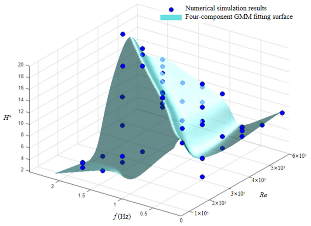
Unlike earlier studies that primarily examined individual operating conditions [21,24], the present model provides a preliminary quantitative mapping of the critical wall distance over the investigated $Re$-$f$ parameter space. Figure 19 presents the fitting results of the four-component Gaussian mixture model for the coupled relationship where the blue scattered points represent raw numerical simulation data, and the cyan surface denotes the model prediction. The results demonstrate that the model provides an empirical and preliminary mapping over the investigated $Re$ or $f$ parameter space, providing a quantitative basis for experimental parameter selection of the oscillating hydrofoil, with promising prospects for engineering design and experimental guidance.

5. Conclusions

This work develops a numerical model of the oscillating hydrofoil under bilateral wing-in-ground (WIG) effect. The influences of the dimensionless wall distance, the oscillation frequency and the Reynolds number on the energy harvesting performance of the oscillating hydrofoil are systematically investigated. A prediction model for the wall distance at which the WIG effect becomes negligible under different combinations of Reynolds number and oscillation frequency is constructed. It provides a quantitative basis for avoiding WIG effect interference in relevant experimental investigations.

The results show that wall distance plays a significant regulatory role in the hydrofoil’s energy harvesting performance. As the wall distance increases, the energy harvesting efficiency decreases monotonically with a gradually reduced rate of decline. At $H^{\ast }=9$, the energy harvesting efficiency is 39.8%, which differs by 5.3% from the value at $H^{\ast }=40$. This condition can approximately be considered free from the WIG effect. The energy harvesting efficiency exhibits a double-peak distribution with $f^{*}$. A primary peak appears near $f^{*}=0.12$, followed by the secondary peak near $f^{*}=0.2$. As $f^{*}$ increases, the hydrofoil becomes more sensitive to the WIG effect, and the wall constraint becomes more pronounced. Variations in the Reynolds number significantly affect the hydrofoil flow regime and harvesting efficiency. As $Re$ increases, viscous effects weaken and the flow field becomes fully developed, leading to a substantial improvement in energy harvesting efficiency. The influence of the WIG effect on energy harvesting first decreases with increasing $Re$, then increases after $Re=4.5\times {10}^5$.

The coupling between the Reynolds number and the oscillation frequency alters the effective angle of attack and vortex evolution behavior, directly affecting force characteristics and energy harvesting. There is a nonlinear coupling effect between the Reynolds number and the oscillation frequency. Accordingly, the four-component Gaussian mixture model is constructed based on orthogonal experimental data to predict the wall distance at which the WIG effect becomes negligible under different conditions. This provides a quantitative basis for avoiding the WIG effect interference in oscillating hydrofoil experiments.

Several limitations of the present study should be acknowledged. First, the numerical simulations are performed using a two-dimensional URANS model, which cannot fully capture inherently three-dimensional flow characteristics, including spanwise vortex evolution, finite-span tip effects, and complex vortex deformation. Although the present model provides an efficient framework for identifying the critical wall distance and its dependence on the governing parameters, three-dimensional simulations are required in future work to further quantify these effects. Second, the present study is intended as a preliminary numerical investigation to establish the parameter mapping and identify the critical operating conditions associated with vortex suppression. The obtained results provide a theoretical basis and parameter guidance for subsequent experimental investigations, through which the predicted critical wall distances and the underlying flow mechanisms will be systematically validated under practical operating conditions.