Contraction-Based Trajectory Tracking Control for AUVs on SE(3) with Hierarchical Gain Certification

Abstract

This paper develops a contraction-certified trajectory-tracking and gain-selection framework for fully actuated autonomous underwater vehicles on $SE\left(3\right)$. The vehicle dynamics are represented in port-Hamiltonian form with a Rayleigh-type dissipation potential, and a dual potential shaping controller provides an energy-structured rotational–translational cascade. Regional contraction certificates are derived separately for the rotational and translational subsystems. The rotational analysis uses fixed left-trivialised momentum coordinates and retains anisotropic-inertia effects and the complete off-diagonal differential coupling. The translational analysis applies to a general known symmetric positive-definite inertia matrix through an attitude-cover semidefinite programme, with an exact endpoint reduction for isotropic inertia. A scaled composite metric combines the subsystem certificates and guarantees every strict complete-cascade rate below the slower subsystem rate. Large initial attitude errors are handled by an energy-entry phase followed by contraction within a prescribed tube, without controller switching. The four-dimensional gain-selection problem is decomposed into two independent two-dimensional offline searches using bisection and SDP/LMI feasibility tests. Numerical studies on the ODIN AUV quantify the region–gain–rate trade-off and examine small-angle, large-angle, and near-antipodal manoeuvres. The framework certifies complete-cascade rates of $0.042096{\mathrm{s}}^{-1}$ and $0.008524{\mathrm{s}}^{-1}$ for the ${60}^{\circ }/{60}^{\circ }$ and ${150}^{\circ }/{80}^{\circ }$ regions, respectively.

1. Introduction

Autonomous underwater vehicles (AUVs) are subject to coupled rotational and translational dynamics with pronounced hydrodynamic nonlinearities, including added-mass effects, Coriolis and centripetal forces, hydrostatic restoring forces, and velocity-dependent drag. These physical effects have a natural energy-based interpretation: the total mechanical energy decomposes into kinetic and potential contributions, while hydrodynamic drag acts as a dissipation mechanism. The port-Hamiltonian (pH) framework captures this structure explicitly, representing energy storage through the Hamiltonian, power-conserving exchange through the interconnection structure, dissipation through the resistive structure, and actuation through the input map [1]. This framework provides a useful basis for AUV modelling and control because stability properties can be related directly to energy flow and the physical structure of the dynamics.

Building on the pH modelling structure, interconnection and damping assignment passivity-based control (IDA-PBC) stabilises a system by shaping its Hamiltonian and assigning the closed-loop interconnection and damping structures while preserving passivity [2,3,4,5]. Marine applications include vessel dynamic positioning with integral action [6] and AUV steering stabilisation [7]. Extending energy-shaping methods from regulation to trajectory tracking is more involved because a moving reference yields a non-autonomous closed loop and a time-dependent target energy. Generalised canonical transformations, extended-state formulations, and error-state IDA-PBC schemes have been developed to address this issue [8,9,10,11]. These studies establish that passive trajectory tracking can be achieved within the pH framework. Their principal objectives are passivity, Lyapunov stability, and disturbance rejection, whereas the present work focuses on prescribed-region contraction certification and automatic gain selection for the complete rotational–translational AUV dynamics.

Geometric tracking control for mechanical systems on manifolds is also well established. Bullo and Murray [12] developed a general tracking framework for fully actuated mechanical systems using intrinsic configuration errors, transport maps, proportional–derivative feedback, and geometric feedforward compensation. Almost-global trajectory tracking was subsequently established for manoeuvrable autonomous vehicles, including AUV models with gravity, buoyancy, hydrodynamic forces, and coupled rigid-body dynamics [13]. Intrinsic PID controllers on Lie groups further extended this viewpoint without relying on local attitude parameterisations [14]. More recent AUV studies have addressed large-angle and fixed-time geometric tracking on $SE\left(3\right)$ under model uncertainty and external disturbances [15]. These developments show that geometric tracking feedback itself is a mature subject. The question considered here is how to certify a quantitative regional convergence rate and select the corresponding gains for the complete AUV rotational–translational cascade.

Contraction theory is well suited to this question because it studies the convergence of neighbouring trajectories rather than only the stability of one equilibrium. Contractive pH and timed IDA-PBC methods have been developed in Euclidean coordinates [16,17,18], while control contraction metrics provide convex conditions for nonlinear feedback design and have recently been extended to systems on Lie groups [19,20]. In an AUV tracking problem on $SE\left(3\right)$, however, the angular and linear momenta are expressed in a moving body frame, the pH interconnection contains momentum-dependent cross-product terms, and the translational variational dynamics are modulated by attitude. Existing results do not directly address this combination of body-fixed momentum transport, Lie-group geometry, and lower-triangular rotational–translational differential coupling.

For attitude systems, Vang and Tron [21] introduced a non-natural cross-coupled metric and converted the resulting contraction condition into an SDP-based gain search for a geometric-PD controller on $SO\left(3\right)$. A subsequent study incorporated a time-varying attitude reference into this framework [22]. Inspired by this certification strategy, the present work develops a hierarchical treatment of the complete AUV tracking cascade. The additional issues are the transported body-fixed momentum, the attitude-dependent translational variational block, and the differential coupling between the rotational and translational subsystems.

The AUV dynamics are represented as a pH system equipped with a Rayleigh-type scalar dissipation potential (PHS-DP). A dual potential shaping control (DPSC) law is then obtained by shaping the desired Hamiltonian and the desired dissipation potential. The desired dissipation potential acts on a transported momentum tracking quantity, and a geometric feedforward term ensures that the feasible reference remains a solution of the original closed-loop vector field. For the fully actuated nominal model and the quadratic desired dissipation potential considered here, the resulting pointwise feedback is algebraically equivalent to a computed-torque geometric-PD controller with the same gains and reference transport. In this setting, the PHS-DP/DPSC construction provides an energy-structured realisation of the tracking dynamics and exposes the cascade structure used in the subsequent certification analysis. The main technical focus is therefore the regional contraction certificate and the associated offline gain-selection procedure.

Given prescribed attitude, momentum, and reference-rate bounds, the design problem is to determine tracking gains and differential metrics that certify a quantitative convergence rate for the complete AUV cascade on $SE\left(3\right)$. The main contributions are as follows.

1.

An energy-structured AUV tracking realisation is formulated on $T^{*}SE\left(3\right)$ using the PHS-DP representation and DPSC construction. The  desired dissipation potential is defined on transported momentum tracking quantities, and the geometric feedforward term enforces reference consistency. The resulting closed-loop dynamics retain the rotational–translational cascade structure required for the contraction analysis.

2.

A hierarchical regional contraction certificate is established for the complete closed loop. The rotational certificate is derived in fixed left-trivialised momentum coordinates while retaining anisotropic-inertia effects and the complete off-diagonal differential block. The translational certificate is stated for a general known symmetric positive-definite inertia matrix through an attitude-cover SDP, with a smaller exact endpoint formulation for isotropic translational inertia. A scaled composite metric combines the two subsystem certificates and yields every strict complete-cascade rate below the slower subsystem rate. Large initial attitude errors are treated by a two-phase result in which an energy argument establishes entry into the contraction region before the complete cascade contracts, without switching the controller.

3.

The gain-certification problem is decomposed into two independent two-dimensional offline searches for $(k_R,k_{\omega })$ and $(k_p,k_v)$. Bisection and SDP/LMI feasibility tests determine the certified rates, controller gains, and metric parameters for each prescribed operating region, thereby establishing a quantitative region–gain–rate relation. Numerical studies on the ODIN AUV examine this trade-off, evaluate the contraction matrices in small- and large-angle manoeuvres, and compare the certified gain selection with independently simulation-tuned geometric-PD gains under the same nominal feedback structure. Tests with model variation, external disturbances, and measurement noise are reported as empirical robustness assessments rather than as a robust contraction proof or experimental validation.

The remainder of this paper is organised as follows. Section 2 reviews pH systems, timed IDA-PBC, and contraction theory. Section 3 formulates the AUV PHS-DP model on $SE\left(3\right)$. Section 4 derives the DPSC tracking law, the hierarchical contraction certificates, and the offline gain-certification procedure. Section 5 presents the nominal, comparative, and non-ideal numerical studies. Section 6 concludes the paper.

2. Preliminaries

2.1. Port-Hamiltonian Systems

Let $\mathcal{X}$ be a smooth n-dimensional manifold. A pH system on $\mathcal{X}$ is defined by the tuple $(\mathcal{J},\mathcal{R},H,\mathcal{G})$ and governed by [1]  

$$\dot{\mathbf{x}}=\left(\mathcal{J}\left(\mathbf{x}\right)-\mathcal{R}\left(\mathbf{x}\right)\right)dH\left(\mathbf{x}\right)+\mathcal{G}\left(\mathbf{x}\right)\mathbf{u},$$

(1a)

$$\mathbf{y}=\mathcal{G}{\left(\mathbf{x}\right)}^{\top }dH\left(\mathbf{x}\right),$$

(1b)

where $H:\mathcal{X}\to \mathbb{R}$ is the Hamiltonian, $\mathbf{u},\mathbf{y}\in {\mathbb{R}}^m$ are conjugate input–output port variables, and $\mathcal{G}\left(\mathbf{x}\right)$ is the input map. The interconnection map $\mathcal{J}\left(\mathbf{x}\right)=-\mathcal{J}{\left(\mathbf{x}\right)}^{\top }$ is skew-symmetric and power-conserving, and the damping map $\mathcal{R}\left(\mathbf{x}\right)=\mathcal{R}{\left(\mathbf{x}\right)}^{\top }⪰\mathbf{0}$ encodes irreversible energy dissipation. The power balance

$$\dot{H}=-dH{\left(\mathbf{x}\right)}^{\top }\mathcal{R}\left(\mathbf{x}\right)dH\left(\mathbf{x}\right)+{\mathbf{y}}^{\top }\mathbf{u}\le {\mathbf{y}}^{\top }\mathbf{u}$$

(2)

confirms passivity with storage function H and supply rate ${\mathbf{y}}^{\top }\mathbf{u}$.

2.2. Timed IDA-PBC for Trajectory Tracking

A trajectory ${\mathbf{x}}^{★}\left(t\right)$ is said to be feasible for system (1) if there exists a control input ${\mathbf{u}}^{★}\left(t\right)$ such that

$${\dot{\mathbf{x}}}^{★}\left(t\right)=\left(\mathcal{J}\left({\mathbf{x}}^{★}\right)-\mathcal{R}\left({\mathbf{x}}^{★}\right)\right)dH\left({\mathbf{x}}^{★}\right)+\mathcal{G}\left({\mathbf{x}}^{★}\right){\mathbf{u}}^{★}\left(t\right),\forall t\ge 0.$$

(3)

The tIDA-PBC method [16,23] seeks a controller such that the closed-loop dynamics take the target form

$$\dot{\mathbf{x}}=({\mathcal{J}}_d-{\mathcal{R}}_d)d{H}_d(\mathbf{x},{\mathbf{x}}^{★}\left(t\right)),$$

(4)

where ${\mathcal{J}}_d=-{\mathcal{J}}_d^{\top }$ and ${\mathcal{R}}_d={\mathcal{R}}_d^{\top }⪰\mathbf{0}$ are constant desired interconnection and damping matrices, and $H_d:\mathcal{X}\times \mathcal{X}\to \mathbb{R}$ is a time-varying desired Hamiltonian. For  ${\mathbf{x}}^{★}\left(t\right)$ to be a solution of (4), the consistency condition

$${\dot{\mathbf{x}}}^{★}\left(t\right)=({\mathcal{J}}_d-{\mathcal{R}}_d)d{H}_d({\mathbf{x}}^{★}\left(t\right),{\mathbf{x}}^{★}\left(t\right))$$

(5)

must hold for all $t\ge 0$. The desired Hamiltonian $H_d$ is further required to satisfy the uniform convexity condition

$${\alpha }_1\mathbf{I}\prec {\nabla }^2{H}_d(\mathbf{x},{\mathbf{x}}^{★}\left(t\right))\prec {\alpha }_2\mathbf{I},\forall \mathbf{x}\in {\mathcal{D}}_T,\forall t\ge 0,$$

(6)

for constants $0<{\alpha }_1<{\alpha }_2$, where ${\mathcal{D}}_T$ is an open neighbourhood of ${\mathbf{x}}^{★}\left(t\right)$.

Theorem 1

(tIDA-PBC [16,23]). Let ${\mathbf{x}}^{★}\left(t\right)$ be a feasible trajectory for (1). Suppose there exist constant matrices ${\mathcal{J}}_d$, ${\mathcal{R}}_d$ and a function $H_d(\mathbf{x},{\mathbf{x}}^{★}\left(t\right))$ satisfying (5) and (6) such that ${\mathcal{J}}_d-{\mathcal{R}}_d$ is Hurwitz and the matching equation

$${\mathcal{G}}^{\perp }\left(\mathbf{x}\right)\left(\mathcal{J}\left(\mathbf{x}\right)-\mathcal{R}\left(\mathbf{x}\right)\right)dH\left(\mathbf{x}\right)={\mathcal{G}}^{\perp }\left(\mathbf{x}\right)\left({\mathcal{J}}_d-{\mathcal{R}}_d\right)d{H}_d(\mathbf{x},{\mathbf{x}}^{★}\left(t\right))$$

(7)

holds, where ${\mathcal{G}}^{\perp }$ is a full-rank left annihilator of $\mathcal{G}$. Then, the control law

$$\mathbf{u}={\mathcal{G}}^{†}\left[\left({\mathcal{J}}_d-{\mathcal{R}}_d\right)d{H}_d(\mathbf{x},{\mathbf{x}}^{★}\left(t\right))-\left(\mathcal{J}\left(\mathbf{x}\right)-\mathcal{R}\left(\mathbf{x}\right)\right)dH\left(\mathbf{x}\right)\right]$$

(8)

renders ${\mathbf{x}}^{★}\left(t\right)$ an exponential tracker for all initial conditions in ${\mathcal{D}}_T$, where ${\mathcal{G}}^{†}$ denotes the Moore–Penrose pseudoinverse of $\mathcal{G}$.

Here, exponential tracking means that there exist constants $C\ge 1$ and $\lambda >0$ such that, for a local distance $d_T$ on ${\mathcal{D}}_T$,

$$d_T(\mathbf{x}\left(t\right),{\mathbf{x}}^{★}\left(t\right))\le C{e}^{-\lambda (t-t_0)}{d}_T(\mathbf{x}\left(t_0\right),{\mathbf{x}}^{★}\left(t_0\right)).$$

2.3. Contraction Theory

Consider a continuously differentiable system $\dot{\mathbf{x}}=f(\mathbf{x},t)$ with variational displacement $\delta \dot{\mathbf{x}}=(\mathsf{\partial }f/\mathsf{\partial }\mathbf{x})\delta \mathbf{x}$. Throughout this paper, the contraction rate $\beta$ denotes the exponential decay rate of the differential norm, not of its square.

Proposition 1

(Euclidean contraction [24]). The system is contracting at rate $\beta >0$ in a constant metric $\mathbf{P}={\mathbf{P}}^{\top }\succ \mathbf{0}$ if

$${\left({\displaystyle \frac{\mathsf{\partial }f}{\mathsf{\partial }\mathbf{x}}}\right)}^{\top }\mathbf{P}+\mathbf{P}{\displaystyle \frac{\mathsf{\partial }f}{\mathsf{\partial }\mathbf{x}}}⪯-2\beta \mathbf{P}.$$

(9)

Then

$${\parallel \delta \mathbf{x}\left(t\right)\parallel }_{\mathbf{P}}\le e^{-\beta (t-t_0)}{\parallel \delta \mathbf{x}\left(t_0\right)\parallel }_{\mathbf{P}}.$$

For a system on a smooth manifold $\mathcal{X}$, let g be a Riemannian metric, ∇ its Levi–Civita connection, and $d_g$ the induced distance. A set is K-reachable if any two of its points can be connected inside the set by a differentiable curve whose length is at most K times their distance.

Proposition 2

(Manifold contraction [25]). Let $\mathcal{C}\subset \mathcal{X}$ be connected, forward invariant, K-reachable, and forward complete. If 

$$g({\nabla }_{\delta \mathbf{x}}f,\delta \mathbf{x})\le -\beta g(\delta \mathbf{x},\delta \mathbf{x})$$

(10)

holds for every $\mathbf{x}\in \mathcal{C}$, time t, and tangent vector $\delta \mathbf{x}$, then any two solutions that remain in $\mathcal{C}$ satisfy

$$d_g({\mathbf{x}}_1\left(t\right),{\mathbf{x}}_2\left(t\right))\le K{e}^{-\beta (t-t_0)}{d}_g({\mathbf{x}}_1\left(t_0\right),{\mathbf{x}}_2\left(t_0\right)).$$

(11)

A time-dependent invertible differential transformation $\mathit{\xi }=\mathbf{T}(\mathbf{x},t)\delta \mathbf{x}$ produces the generalised Jacobian

$$\mathbf{F}=\dot{\mathbf{T}}{\mathbf{T}}^{-1}+\mathbf{T}{\displaystyle \frac{\mathsf{\partial }f}{\mathsf{\partial }\mathbf{x}}}{\mathbf{T}}^{-1}.$$

(12)

A constant metric $\mathbf{G}$ in $\mathit{\xi }$ coordinates is equivalent to the pullback metric $\mathbf{P}(\mathbf{x},t)={\mathbf{T}}^{\top }\mathbf{G}\mathbf{T}$ in the original tangent coordinates. This observation is used only for the translational variational displacement in Section 4.2.2; the nonlinear closed-loop state is not replaced by an error system.

Consider the lower-triangular variational system

$$\left(\begin{array}{c}{\dot{\mathit{\xi }}}_1\\ {\dot{\mathit{\xi }}}_2\end{array}\right)=\left(\begin{array}{cc}{\mathbf{F}}_1& \mathbf{0}\\ {\mathbf{B}}_{21}& {\mathbf{F}}_2\end{array}\right)\left(\begin{array}{c}{\mathit{\xi }}_1\\ {\mathit{\xi }}_2\end{array}\right).$$

(13)

If the diagonal subsystems contract uniformly and ${\mathbf{B}}_{21}$ is bounded, a scaled block metric establishes contraction of the cascade [25,26]. In general, every strict rate below the minimum of the two subsystem rates can be attained; the minimum itself need not be attained when ${\mathbf{B}}_{21}\ne \mathbf{0}$. A quantitative version is proved in Theorem 2.

3. PHS-DP Modelling of AUVs on $\mathit{SE}\left(\mathbf{3}\right)$

The standard six-degree-of-freedom (6-DoF) AUV model [27] employs Euler angles, introducing kinematic singularities that complicate geometric control design. We formulate the AUV dynamics as a PHS-DP directly on $SE\left(3\right)$, avoiding these singularities while retaining the physical transparency of the energy-based structure. The vectorised configuration representation follows the $SE\left(3\right)$ rigid-body framework of Duong et al. [28]; the hydrostatic potential, hydrodynamic dissipation, and AUV-specific physical parameters are introduced here.

3.1. Configuration and Kinematics on $SE\left(3\right)$

The configuration of an AUV is an element of

$$SE\left(3\right)=\left\{\left[\begin{array}{cc}\mathbf{R}& \mathbf{p}\\ {\mathbf{0}}^{\top }& 1\end{array}\right]:\mathbf{R}\in SO\left(3\right),\mathbf{p}\in {\mathbb{R}}^3\right\},$$

(14)

where $\mathbf{R}$ is the rotation matrix from the body-fixed frame to the inertial (NED) frame and $\mathbf{p}\in {\mathbb{R}}^3$ is the position of the centre of mass. For compatibility with the PHS-DP formulation, the configuration is vectorised as $\mathfrak{q}={\left[{\mathbf{p}}^{\top }{\mathbf{r}}_1^{\top }{\mathbf{r}}_2^{\top }{\mathbf{r}}_3^{\top }\right]}^{\top }\in {\mathbb{R}}^{12}$, where ${\mathbf{r}}_i\in {\mathbb{R}}^3$ denotes the i-th row of $\mathbf{R}$ as a vector. The body-fixed generalised velocity and momentum are

$$\mathit{\zeta }={\left[\begin{array}{cc}{\mathbf{v}}^{\top }& {\omega }^{\top }\end{array}\right]}^{\top }\in {\mathbb{R}}^6,\mathit{\pi }=\mathbf{M}\mathit{\zeta },\mathbf{M}=\left[\begin{array}{cc}{\mathbf{M}}_v& \mathbf{0}\\ \mathbf{0}& {\mathbf{M}}_{\omega }\end{array}\right]\in {\mathbb{S}}_{\succ 0}^{6\times 6},$$

(15)

where ${\mathbf{M}}_v,{\mathbf{M}}_{\omega }\in {\mathbb{S}}_{\succ 0}^{3\times 3}$ incorporate the rigid-body and added-mass contributions. In this study, the body-fixed origin is placed at the centre of mass, and the total inertia is assumed to admit the block-diagonal form in (15). For the ODIN model used in the numerical study, ${\mathbf{M}}_v=m_v{\mathbf{I}}_3$ and ${\mathbf{M}}_{\omega }$ is diagonal in the selected body axes. The subsequent contraction analysis nevertheless permits each inertia block to be a general known symmetric positive-definite matrix. The vectorised $SE\left(3\right)$ kinematics are

$$\dot{\mathfrak{q}}={\mathfrak{q}}^{\times }\mathit{\zeta },{\mathfrak{q}}^{\times }=\left[\begin{array}{cc}\mathbf{R}& \mathbf{0}\\ \mathbf{0}& {\widehat{\mathbf{r}}}_1\\ \mathbf{0}& {\widehat{\mathbf{r}}}_2\\ \mathbf{0}& {\widehat{\mathbf{r}}}_3\end{array}\right]\in {\mathbb{R}}^{12\times 6},$$

(16)

where $\widehat{(·)}:{\mathbb{R}}^3\to \mathfrak{so}\left(3\right)$ is the hat (skew-symmetric) map, following from $\dot{\mathbf{p}}=\mathbf{R}\mathbf{v}$ and ${\dot{\mathbf{r}}}_i={\widehat{\mathbf{r}}}_i\omega$, the row-wise form of $\dot{\mathbf{R}}=\mathbf{R}\widehat{\omega }$.

3.2. AUV Dynamics as a PHS-DP

In the PHS-DP representation used here, the hydrodynamic dissipative force is generated by the momentum gradient of a scalar dissipation potential ${\mathcal{F}}_p$ on the cotangent bundle $T^{*}\mathcal{Q}$, rather than written directly as a resistive matrix acting on the Hamiltonian gradient. The dynamics are governed by

$$\left(\begin{array}{c}\dot{\mathfrak{q}}\\ \dot{\mathit{\pi }}\end{array}\right)=\mathcal{J}\left(\begin{array}{c}{\nabla }_{\mathfrak{q}}H\\ {\nabla }_{\mathit{\pi }}H\end{array}\right)-\left(\begin{array}{c}\mathbf{0}\\ {\nabla }_{\mathit{\pi }}{\mathcal{F}}_p\end{array}\right)+\left(\begin{array}{c}\mathbf{0}\\ {\mathbf{I}}_6\end{array}\right)\mathbf{u},$$

(17a)

$$\mathbf{y}={\nabla }_{\mathit{\pi }}H,$$

(17b)

where ${\mathcal{F}}_p$ satisfies

$${\nabla }_{\mathit{\pi }}{\mathcal{F}}_p\left(\mathbf{0}\right)=\mathbf{0},{\nabla }_{\mathit{\pi }}{\mathcal{F}}_p{\left(\mathit{\pi }\right)}^{\top }\mathit{\zeta }>0,\forall \mathit{\pi }\ne \mathbf{0},$$

(18)

ensuring zero dissipation at rest and strictly positive power dissipation during motion. The skew-symmetric interconnection matrix is

$$\mathcal{J}=\left[\begin{array}{cc}{\mathbf{0}}_{12\times 12}& {\mathfrak{q}}^{\times }\\ -{\left({\mathfrak{q}}^{\times }\right)}^{\top }& {\mathit{\pi }}^{\times }\end{array}\right],$$

(19)

where ${\mathit{\pi }}_v={\mathbf{M}}_v\mathbf{v}$, ${\mathit{\pi }}_{\omega }={\mathbf{M}}_{\omega }\omega$, and 

$${\mathit{\pi }}^{\times }=\left[\begin{array}{cc}{\mathbf{0}}_{3\times 3}& {\widehat{\mathit{\pi }}}_v\\ {\widehat{\mathit{\pi }}}_v& {\widehat{\mathit{\pi }}}_{\omega }\end{array}\right]\in {\mathbb{R}}^{6\times 6},$$

(20)

whose action on $\mathit{\zeta }={\mathbf{M}}^{-1}\mathit{\pi }$ gives the Coriolis–centripetal term

$${\mathit{\pi }}^{\times }{\mathbf{M}}^{-1}\mathit{\pi }=\left[\begin{array}{c}{\mathit{\pi }}_v\times \omega \\ {\mathit{\pi }}_v\times \mathbf{v}+{\mathit{\pi }}_{\omega }\times \omega \end{array}\right].$$

(21)

Let ${\mathbf{r}}_{gb}\in {\mathbb{R}}^3$ denote the position of the centre of buoyancy relative to the centre of gravity in body-fixed coordinates [27]. The total mechanical energy is

$$H=\frac{1}{2}{\mathit{\pi }}^{\top }{\mathbf{M}}^{-1}\mathit{\pi }+V\left(\mathfrak{q}\right),$$

(22)

with hydrostatic potential

$$V\left(\mathfrak{q}\right)=(B-W){\mathbf{e}}_3^{\top }\mathbf{p}+B{\mathbf{e}}_3^{\top }\left(\mathbf{R}{\mathbf{r}}_{gb}\right),$$

(23)

where $W=mg$, $B=\rho g{V}_{\mathrm{disp}}$, and ${\mathbf{e}}_3={[0,0,1]}^{\top }$ is the unit vector along the NED downward axis. The first term accounts for the net buoyancy force acting on the centre of mass; the second encodes the hydrostatic restoring moment due to the offset ${\mathbf{r}}_{gb}$. Since ${\mathbf{e}}_3^{\top }\left(\mathbf{R}{\mathbf{r}}_{gb}\right)={\mathbf{r}}_3^{\top }{\mathbf{r}}_{gb}$, only the third row ${\mathbf{r}}_3$ of $\mathbf{R}$ enters V, giving

$${\displaystyle \frac{\mathsf{\partial }V}{\mathsf{\partial }\mathbf{p}}}=(B-W){\mathbf{e}}_3,{\displaystyle \frac{\mathsf{\partial }V}{\mathsf{\partial }{\mathbf{r}}_i}}=B{\delta }_{i3}{\mathbf{r}}_{gb},$$

(24)

where ${\delta }_{i3}$ is the Kronecker delta. Substituting into ${\tau }_g=-{\left({\mathfrak{q}}^{\times }\right)}^{\top }{\nabla }_{\mathfrak{q}}V$ and using ${\widehat{\mathbf{r}}}_i^{\top }=-{\widehat{\mathbf{r}}}_i$ yields

$${\tau }_g=\left[\begin{array}{c}(W-B){\mathbf{R}}^{\top }{\mathbf{e}}_3\\ -{\mathbf{r}}_{gb}\times \left(B{\mathbf{R}}^{\top }{\mathbf{e}}_3\right)\end{array}\right],$$

(25)

consistent with the standard hydrostatic model [27].

Hydrodynamic drag is encoded through

$${\mathcal{F}}_p\left(\mathit{\pi }\right)=\frac{1}{2}{\mathit{\pi }}^{\top }{\mathbf{D}}_L{\mathbf{M}}^{-1}\mathit{\pi }+\frac{1}{3}{\mathit{\pi }}^{\top }{\mathbf{D}}_Q\left(\mathit{\zeta }\right){\mathbf{M}}^{-1}\mathit{\pi },$$

(26)

where

$$\begin{array}{cc}\hfill {\mathbf{D}}_L& =\mathrm{blkdiag}\left(\mathrm{diag}\left(d_{L,v}^{\left(i\right)}\right),\mathrm{diag}\left(d_{L,\omega }^{\left(j\right)}\right)\right)⪰\mathbf{0},\hfill \\ \hfill {\mathbf{D}}_Q\left(\mathit{\zeta }\right)& =\mathrm{blkdiag}\left(\mathrm{diag}(d_{Q,v}^{\left(i\right)}|v_i|),\mathrm{diag}(d_{Q,\omega }^{\left(j\right)}|{\omega }_j|)\right)⪰\mathbf{0}.\hfill \end{array}$$

(27)

The dissipation gradient is ${\nabla }_{\mathit{\pi }}{\mathcal{F}}_p=({\mathbf{D}}_L+{\mathbf{D}}_Q\left(\mathit{\zeta }\right))\mathit{\zeta }$, and the power dissipation

$$\begin{array}{cc}\hfill {\nabla }_{\mathit{\pi }}{\mathcal{F}}_p^{\top }\mathit{\zeta }=& \sum _i{d}_{L,v}^{\left(i\right)}{v}_i^2+\sum _j{d}_{L,\omega }^{\left(j\right)}{\omega }_j^2\hfill \\ & +\sum _i{d}_{Q,v}^{\left(i\right)}|v_i{|}^3+\sum _j{d}_{Q,\omega }^{\left(j\right)}{|{\omega }_j|}^3\hfill \end{array}$$

(28)

is strictly positive for all $\mathit{\pi }\ne \mathbf{0}$ provided that each velocity direction has a strictly positive linear or quadratic drag coefficient, which is satisfied by the ODIN parameters used below. This verifies (18).

Substituting (22)–(26) into (17) yields the explicit equations of motion   

$$\dot{\mathfrak{q}}={\mathfrak{q}}^{\times }{\mathbf{M}}^{-1}\mathit{\pi },$$

(29a)

$$\dot{\mathit{\pi }}={\mathit{\pi }}^{\times }{\mathbf{M}}^{-1}\mathit{\pi }+{\mathit{\tau }}_g-\left({\mathbf{D}}_L+{\mathbf{D}}_Q\left(\mathit{\zeta }\right)\right)\mathit{\zeta }+\mathbf{u}.$$

(29b)

4. DPSC Trajectory Tracking Control

This section develops the DPSC control law for trajectory tracking of the AUV PHS-DP model (29). A reference trajectory $({\mathfrak{q}}^{*}\left(t\right),{\mathit{\pi }}^{*}\left(t\right))$ on $T^{*}SE\left(3\right)$ is feasible for (29) if there exists ${\mathbf{u}}^{*}\left(t\right)$ such that (29) holds at $({\mathfrak{q}}^{*},{\mathit{\pi }}^{*})$ for all $t\ge 0$, with ${\mathit{\pi }}^{*}\left(t\right)=\mathbf{M}{\mathit{\zeta }}^{*}\left(t\right)$. The control design proceeds in three steps: (i) potential energy shaping to encode the configuration error; (ii) dissipation potential shaping on the momentum error; (iii) a geometric feedforward term, derived from the consistency condition, that accounts for the time variation of the transported reference momentum. Here, ${(·)|}^{*}$ denotes evaluation at $({\mathfrak{q}}^{*},{\mathit{\pi }}^{*})$.

4.1. DPSC Control Law and Closed-Loop Dynamics

The desired Hamiltonian retains the kinetic energy and shapes the potential to encode the configuration error:

$$H_d(\mathfrak{q},\mathit{\pi },t)=\frac{1}{2}{\mathit{\pi }}^{\top }{\mathbf{M}}^{-1}\mathit{\pi }+\frac{1}{2}{k}_p{\parallel \mathbf{p}-{\mathbf{p}}^{*}\parallel }^2+k_R\mathrm{\Psi }(\mathbf{R},{\mathbf{R}}^{*}),$$

(30)

where $k_p,k_R>0$, and the attitude error function is [29]

$$\mathrm{\Psi }(\mathbf{R},{\mathbf{R}}^{*})=2-\sqrt{1+\mathrm{tr}\left({\mathbf{R}}^{*\top }\mathbf{R}\right)}.$$

(31)

Let $Q\triangleq {\mathbf{R}}^{\top }{\mathbf{R}}^{*}\in SO\left(3\right)$ denote the relative attitude and $\theta \in [0,\mathit{\pi })$ the corresponding geodesic angle, so that $\mathrm{tr}\left(Q\right)=\mathrm{tr}\left({\mathbf{R}}^{*\top }\mathbf{R}\right)$ and $\mathrm{\Psi }=4{sin}^2(\theta /4)$. The left-trivialised gradient of $\mathrm{\Psi }$ with respect to $\mathbf{R}$ is the attitude error vector

$${\mathbf{e}}_R={\displaystyle \frac{{(Q^{\top }-Q)}^{\vee }}{2\sqrt{1+\mathrm{tr}\left(Q\right)}}},\parallel {\mathbf{e}}_R\parallel =sin\frac{\theta }{2},$$

(32)

well defined on ${\mathcal{L}}_2=\{\mathbf{R}\in SO\left(3\right)\mid \mathrm{\Psi }<2\}$, i.e., for $\theta \in [0,\mathit{\pi })$. The shaped potential satisfies ${\nabla }_{\mathbf{p}}{H}_d{|}_{{\mathbf{p}}^{*}}=\mathbf{0}$, ${\nabla }_{\mathbf{p}}^2{H}_d=k_p{\mathbf{I}}_3\succ \mathbf{0}$, and ${\mathbf{R}}^{*}\left(t\right)$ is the unique strict local minimum of $\mathrm{\Psi }(·,{\mathbf{R}}^{*})$ within ${\mathcal{L}}_2$.

Since $\mathit{\pi }=\mathbf{M}\mathit{\zeta }$ is expressed in the current body frame and ${\mathit{\pi }}^{*}=\mathbf{M}{\mathit{\zeta }}^{*}$ in the reference body frame, they belong to different cotangent spaces and cannot be compared directly. The  reference velocity is transported to the current body frame via Q:

$${\overline{\mathit{\zeta }}}^{*}\triangleq \left[\begin{array}{c}{\mathbf{R}}^{\top }{\dot{\mathbf{p}}}^{*}\\ Q{\omega }^{*}\end{array}\right],{\overline{\mathit{\pi }}}^{*}\triangleq \mathbf{M}{\overline{\mathit{\zeta }}}^{*},$$

(33)

where ${\mathbf{R}}^{\top }{\dot{\mathbf{p}}}^{*}=Q{\mathbf{v}}^{*}$ is the reference linear velocity expressed in the current body frame. The momentum tracking error is

$${\mathbf{e}}_{\mathit{\pi }}\triangleq \mathit{\pi }-{\overline{\mathit{\pi }}}^{*}=\left[\begin{array}{c}{\mathbf{M}}_v{\mathbf{e}}_v\\ {\mathbf{M}}_{\omega }{\mathbf{e}}_{\omega }\end{array}\right],$$

(34)

where ${\mathbf{e}}_v\triangleq \mathbf{v}-{\mathbf{R}}^{\top }{\dot{\mathbf{p}}}^{*}$ and ${\mathbf{e}}_{\omega }\triangleq \omega -Q{\omega }^{*}$ are the body-frame velocity errors. The desired dissipation potential is defined on the momentum error:

$${\mathcal{F}}_d(\mathfrak{q},\mathit{\pi },t)=\frac{1}{2}{\mathbf{e}}_{\mathit{\pi }}^{\top }{\mathbf{D}}_d{\mathbf{M}}^{-1}{\mathbf{e}}_{\mathit{\pi }},{\mathbf{D}}_d=\mathrm{blkdiag}(k_v{\mathbf{I}}_3,k_{\omega }{\mathbf{I}}_3)\succ \mathbf{0},$$

(35)

with $k_v,k_{\omega }>0$. Its gradient satisfies ${\nabla }_{\mathit{\pi }}{\mathcal{F}}_d={\mathbf{D}}_d{\mathbf{M}}^{-1}{\mathbf{e}}_{\mathit{\pi }}$, which vanishes when the momentum error is zero, rather than when the absolute momentum is zero.

Since ${\overline{\mathit{\pi }}}^{*}$ depends on $\mathfrak{q}$ through $Q={\mathbf{R}}^{\top }{\mathbf{R}}^{*}$, its time derivative along the closed loop is the transport derivative

$${\dot{\overline{\mathit{\pi }}}}^{*}=\mathbf{M}\left[\begin{array}{c}{\mathbf{R}}^{\top }{\ddot{\mathbf{p}}}^{*}-\widehat{\omega }{\mathbf{R}}^{\top }{\dot{\mathbf{p}}}^{*}\\ Q{\dot{\omega }}^{*}-\widehat{\omega }Q{\omega }^{*}\end{array}\right],$$

(36)

obtained from $\dot{Q}=-\widehat{\omega }Q+Q{\widehat{\omega }}^{*}$ and ${\dot{\mathbf{R}}}^{\top }=-\widehat{\omega }{\mathbf{R}}^{\top }$. The correction terms $-\widehat{\omega }{\mathbf{R}}^{\top }{\dot{\mathbf{p}}}^{*}$ and $-\widehat{\omega }Q{\omega }^{*}$ arise from differentiating the transported reference quantities in the rotating body frame. The desired closed-loop momentum dynamics are

$$\dot{\mathit{\pi }}=-{\left({\mathfrak{q}}^{\times }\right)}^{\top }{\nabla }_{\mathfrak{q}}{H}_d-{\mathbf{D}}_d{\mathbf{M}}^{-1}{\mathbf{e}}_{\mathit{\pi }}+{\dot{\overline{\mathit{\pi }}}}^{*},$$

(37)

so that the momentum error evolves as

$${\dot{\mathbf{e}}}_{\mathit{\pi }}=-{\left({\mathfrak{q}}^{\times }\right)}^{\top }{\nabla }_{\mathfrak{q}}{H}_d-{\mathbf{D}}_d{\mathbf{M}}^{-1}{\mathbf{e}}_{\mathit{\pi }}.$$

(38)

At $(\mathfrak{q},\mathit{\pi })=({\mathfrak{q}}^{*},{\mathit{\pi }}^{*})$, we have ${\mathbf{e}}_{\mathit{\pi }}=\mathbf{0}$ and ${\nabla }_{\mathfrak{q}}{H}_d{|}^{*}=\mathbf{0}$ since $\mathbf{p}={\mathbf{p}}^{*}$ and $\mathbf{R}={\mathbf{R}}^{*}$ imply ${\mathbf{e}}_R=\mathbf{0}$, so Equation (37) reduces to ${\dot{\mathit{\pi }}}^{*}={\dot{\overline{\mathit{\pi }}}}^{*}{|}^{*}$, confirming that the consistency condition (3) is satisfied without residual. Equating (37) with the open-loop dynamics (29b) and solving for $\mathbf{u}$ gives the DPSC control law

$$\mathbf{u}=-\left[\begin{array}{c}{k}_p{\mathbf{R}}^{\top }(\mathbf{p}-{\mathbf{p}}^{*})\\ k_R{\mathbf{e}}_R\end{array}\right]-{\mathbf{D}}_d{\mathbf{M}}^{-1}{\mathbf{e}}_{\mathit{\pi }}+{\dot{\overline{\mathit{\pi }}}}^{*}+{\left({\mathfrak{q}}^{\times }\right)}^{\top }{\nabla }_{\mathfrak{q}}V-{\mathit{\pi }}^{\times }{\mathbf{M}}^{-1}\mathit{\pi }+{\nabla }_{\mathit{\pi }}{\mathcal{F}}_p.$$

(39)

Substituting (39) into (29) yields the closed-loop equations

$$\dot{\mathbf{R}}=\mathbf{R}\widehat{\omega },$$

(40a)

$${\dot{\mathit{\pi }}}_{\omega }=-k_R{\mathbf{e}}_R-k_{\omega }{\mathbf{e}}_{\omega }+{\mathbf{M}}_{\omega }(Q{\dot{\omega }}^{*}-\widehat{\omega }Q{\omega }^{*}),$$

(40b)

$$\dot{\mathbf{p}}=\mathbf{R}\mathbf{v},$$

(40c)

$${\dot{\mathit{\pi }}}_v=-k_p{\mathbf{R}}^{\top }(\mathbf{p}-{\mathbf{p}}^{*})-k_v{\mathbf{e}}_v+{\mathbf{M}}_v({\mathbf{R}}^{\top }{\ddot{\mathbf{p}}}^{*}-\widehat{\omega }{\mathbf{R}}^{\top }{\dot{\mathbf{p}}}^{*}).$$

(40d)

Proposition 3

(Reference consistency). The feasible reference $({\mathfrak{q}}^{*},{\mathit{\pi }}^{*})$ is a solution of the original closed-loop dynamics (40).

Proof. 

At the reference, $\mathbf{Q}={\mathbf{I}}_3$, ${\mathbf{e}}_{\mathit{\pi }}=\mathbf{0}$, ${\mathbf{e}}_R=\mathbf{0}$, and ${\overline{\mathit{\pi }}}^{*}={\mathit{\pi }}^{*}$. Moreover, ${\dot{\overline{\mathit{\pi }}}}^{*}={\dot{\mathit{\pi }}}^{*}$ along the reference. Substitution in (37) and the original kinematics gives the prescribed reference dynamics without a residual.    □

4.2. Contraction Analysis

The contraction analysis is performed directly on the original closed-loop state in (40); no nonlinear tracking-error system is introduced as a replacement model. The closed loop has the cascade form

$${\displaystyle \frac{d}{dt}}\left(\begin{array}{c}{\mathbf{x}}_R\\ {\mathbf{x}}_v\end{array}\right)=\left(\begin{array}{c}{f}_R({\mathbf{x}}_R,t)\\ f_v({\mathbf{x}}_R,{\mathbf{x}}_v,t)\end{array}\right),$$

(41)

where

$${\mathbf{x}}_R=(\mathbf{R},{\mathit{\pi }}_{\omega })\in SO\left(3\right)\times {\mathbb{R}}^3,{\mathbf{x}}_v=(\mathbf{p},{\mathit{\pi }}_v)\in {\mathbb{R}}^6,$$

and $f_R$ is independent of ${\mathbf{x}}_v$. The proof is organised as follows. First, a Vang-inspired cross-coupled differential metric in fixed left-trivialised momentum coordinates is used to certify the rotational subsystem. Second, the translational subsystem is shown to be partially contracting, uniformly with respect to the rotational input. Finally, the bounded lower-triangular differential coupling is absorbed by a scaled composite metric.

4.2.1. Rotational Subsystem

The rotational subsystem is represented by the state $(\mathbf{R},{\mathit{\pi }}_{\omega })\in SO\left(3\right)\times {\mathbb{R}}^3$. Although the physical model is written in angular-momentum coordinates, the differential analysis uses a fixed left-trivialised body-coordinate representation of the angular-momentum fibre. The resulting certificate is therefore tied to the adopted momentum coordinates and is not claimed to be invariant under arbitrary cotangent-fibre reparameterisations. Define

$${\overline{\mathit{\omega }}}^{*}\triangleq \mathbf{Q}{\mathit{\omega }}^{*},{\overline{\dot{\mathit{\omega }}}}^{*}\triangleq \mathbf{Q}{\dot{\mathit{\omega }}}^{*},{\overline{\mathit{\pi }}}_{\mathit{\omega }}^{*}={\mathbf{M}}_{\omega }{\overline{\mathit{\omega }}}^{*},$$

(42)

where $\mathbf{Q}={\mathbf{R}}^{\top }{\mathbf{R}}^{*}$. The corresponding closed-loop vector field can be written as

$$\overline{X}=\left(\mathbf{R}\widehat{\mathit{\omega }},\mathbf{R}\widehat{\mathit{\vartheta }}\right),$$

(43)

with

$$\begin{array}{cc}\hfill \mathit{\vartheta }& =-k_R{\mathbf{e}}_R-k_{\omega }{\mathbf{M}}_{\omega }^{-1}({\mathit{\pi }}_{\omega }-{\overline{\mathit{\pi }}}_{\omega }^{*})+{\dot{\overline{\mathit{\pi }}}}_{\omega }^{*},\hfill \\ \hfill {\dot{\overline{\mathit{\pi }}}}_{\omega }^{*}& ={\mathbf{M}}_{\omega }\left({\overline{\dot{\mathit{\omega }}}}^{*}-\widehat{\mathit{\omega }}{\overline{\mathit{\omega }}}^{*}\right).\hfill \end{array}$$

(44)

An arbitrary differential displacement in the same representation is denoted by

$$\overline{Y}=(\mathbf{R}\widehat{\mathit{\zeta }},\mathbf{R}\widehat{\mathit{\eta }}),\mathit{\zeta },\mathit{\eta }\in {\mathbb{R}}^3,$$

where $\mathit{\zeta }$ is the left-trivialised attitude variation and $\mathit{\eta }$ is the corresponding momentum-fibre variation. The notation $\mathbf{R}\widehat{\mathit{\vartheta }}$ and $\mathbf{R}\widehat{\mathit{\eta }}$ is used only as a fixed left-trivialised matrix representation of the momentum-fibre rate and variation; it does not identify the physical momentum fibre with the tangent fibre or alter the nonlinear state space.

Because the two differential coordinates have different physical units, the finite-dimensional certificate is expressed from this point onward in fixed scaled numerical coordinates. The attitude variation is dimensionless, while angular momentum and rotational inertia are represented using the reference units $p_0=1\mathrm{kg}{\mathrm{m}}^2{\mathrm{s}}^{-1}$ and $J_0=1\mathrm{kg}{\mathrm{m}}^2$, respectively. For notational economy, the corresponding dimensionless numerical quantities are denoted by the same symbols. This convention leaves the numerical values used in the implementation unchanged and makes the metric and expressions such as ${\mathbf{M}}_{\omega }-{\mathbf{I}}_3$ dimensionally well defined.

Motivated by the cross-coupled metric structure of Vang [21,30], consider the following positive-definite differential metric in the adopted coordinates:

$$\overline{g}(\overline{Y},\overline{Y})={\left(\begin{array}{c}\mathit{\zeta }\\ \mathit{\eta }\end{array}\right)}^{\top }\underset{{\mathbf{G}}_R}{\underbrace{\left(\begin{array}{cc}{m}_1{\mathbf{I}}_3& m_2{\mathbf{I}}_3\\ m_2{\mathbf{I}}_3& m_3{\mathbf{I}}_3\end{array}\right)}}\left(\begin{array}{c}\mathit{\zeta }\\ \mathit{\eta }\end{array}\right),$$

(45)

where $m_1,m_3>0$ and $m_1{m}_3>m_2^2$, which ensure ${\mathbf{G}}_R\succ 0$. In this paper, the rate ${\beta }_{\omega }$ is the decay rate of the differential norm. A sufficient regional differential contraction condition in the adopted representation is

$$\overline{g}({\overline{\nabla }}_{\overline{Y}}\overline{X},\overline{Y})+{\beta }_{\omega }\overline{g}(\overline{Y},\overline{Y})\le 0.$$

(46)

The factor convention in (46) is consistent with $\parallel \delta \mathbf{x}\left(t\right)\parallel \le e^{-{\beta }_{\omega }(t-t_0)}\parallel \delta \mathbf{x}\left(t_0\right)\parallel$.

The differential of the attitude-gradient vector satisfies

$$\delta {\mathbf{e}}_R=D_{{\mathbf{e}}_R}\mathit{\zeta },D_{{\mathbf{e}}_R}={\displaystyle \frac{tr\left(\mathbf{Q}\right){\mathbf{I}}_3-\mathbf{Q}+2{\mathbf{e}}_R{\mathbf{e}}_R^{\top }}{2\sqrt{1+tr\left(\mathbf{Q}\right)}}}.$$

(47)

For $\mathbf{Q}=exp\left(\theta \widehat{\mathbf{n}}\right)$,

$$D_{{\mathbf{e}}_R}=\mathrm{\Theta }\left(\theta \right){\mathbf{I}}_3+{\displaystyle \frac{1}{2}}{\widehat{\mathbf{e}}}_R,\mathrm{\Theta }\left(\theta \right)={\displaystyle \frac{cos(\theta /2)}{2}},$$

(48)

and hence

$$\mathrm{sym}\left(D_{{\mathbf{e}}_R}\right)=\mathrm{\Theta }\left(\theta \right){\mathbf{I}}_3.$$

(49)

Applying the Vang-inspired horizontal–vertical formulas in the adopted representation to (46) gives

$${\left(\begin{array}{c}\mathit{\zeta }\\ \mathit{\eta }\end{array}\right)}^{\top }\mathrm{sym}\left({\mathcal{M}}_R\right)\left(\begin{array}{c}\mathit{\zeta }\\ \mathit{\eta }\end{array}\right)\le 0,$$

(50)

where the resulting blocks of ${\mathcal{M}}_R$ are derived in Appendix A. Two features must be retained in the anisotropic-inertia analysis. First, $\mathit{\omega }={\mathbf{M}}_{\omega }^{-1}{\mathit{\pi }}_{\omega }$ does not imply that $\mathit{\omega }$ and ${\mathit{\pi }}_{\omega }$ are parallel. Second, the complete off-diagonal block contributes to the spectrum of the symmetric differential matrix and therefore cannot be replaced by its symmetric part alone.

For the finite-dimensional certificate, set $m_1=1$ and define

$$\begin{array}{cccc}\hfill {\mu }_{\omega }& \triangleq {\lambda }_{\max }\left({\mathbf{M}}_{\omega }^{-1}\right),\hfill & \hfill M_{\omega }^{\max }& \triangleq {\lambda }_{\max }\left({\mathbf{M}}_{\omega }\right),\hfill \\ \hfill p_{\max }& \ge \underset{t}{sup}\parallel {\mathit{\pi }}_{\omega }\left(t\right)\parallel ,\hfill & \hfill {\omega }_{\max }^{*}& \ge \underset{t}{sup}\parallel {\mathit{\omega }}^{*}\left(t\right)\parallel ,\hfill \\ \hfill {\mathrm{\Theta }}_{-}& \triangleq {\displaystyle \frac{cos({\theta }_R/2)}{2}},\hfill & \hfill {\delta }_M& \triangleq \parallel {\mathbf{M}}_{\omega }-{\mathbf{I}}_3{\parallel }_2.\hfill \end{array}$$

(51)

The momentum-dependent and mixed-reference contributions satisfy

$${\mathcal{D}}_{\mathrm{\Omega }}\triangleq {\displaystyle \frac{m_2{\mu }_{\omega }}{4}}{p}_{\max }^2+{\displaystyle \frac{m_2{\mu }_{\omega }}{4}}{p}_{\max }+{\displaystyle \frac{m_3{\mu }_{\omega }}{8}}{p}_{\max }^2+{\displaystyle \frac{m_3{k}_{\omega }}{4}}{p}_{\max },$$

(52a)

$${\mathcal{D}}_{\mathrm{\Gamma }}\triangleq {\displaystyle \frac{m_3{M}_{\omega }^{\max }{\mu }_{\omega }}{2}}{p}_{\max }{\omega }_{\max }^{*},$$

(52b)

$$r_P\triangleq {\displaystyle \frac{m_3{k}_{\omega }{\delta }_M}{4}}{\omega }_{\max }^{*}.$$

(52c)

The first term in (52a) uses

$$\widehat{\mathbf{a}}\widehat{\mathbf{b}}+\widehat{\mathbf{b}}\widehat{\mathbf{a}}=\mathbf{a}{\mathbf{b}}^{\top }+\mathbf{b}{\mathbf{a}}^{\top }-2\left({\mathbf{a}}^{\top }\mathbf{b}\right){\mathbf{I}}_3.$$

Its largest eigenvalue is $\parallel \mathbf{a}\parallel \parallel \mathbf{b}\parallel -{\mathbf{a}}^{\top }\mathbf{b}$ and is therefore no greater than $2\parallel \mathbf{a}\parallel \parallel \mathbf{b}\parallel$. Taking $\mathbf{a}=\mathit{\omega }$ and $\mathbf{b}={\mathit{\pi }}_{\omega }$ gives the first term of (52a) without assuming that the two vectors are parallel.

For each endpoint $\mathrm{\Theta }\in \{{\mathrm{\Theta }}_{-},1/2\}$, define the symmetric matrix

$${\mathbf{S}}_R\left(\mathrm{\Theta }\right)\triangleq {\displaystyle \frac{1}{2}}{\mathbf{M}}_{\omega }^{-1}+\left({\beta }_{\omega }{m}_2-{\displaystyle \frac{k_{\omega }{m}_2}{2}}-{\displaystyle \frac{k_R{m}_3\mathrm{\Theta }}{2}}\right){\mathbf{I}}_3.$$

(53)

The complete off-diagonal block is bounded by $\parallel {\mathbf{S}}_R{\left(\mathrm{\Theta }\right)\parallel }_2+r_P$; in particular, the skew reference term is retained through $r_P$. The two block-Gershgorin row bounds are

$${\mathcal{R}}_1\left(\mathrm{\Theta }\right)={\beta }_{\omega }-m_2{k}_R\mathrm{\Theta }+s_{\mathrm{\Theta }}+r_P,$$

(54a)

$${\mathcal{R}}_2\left(\mathrm{\Theta }\right)=m_2{\mu }_{\omega }+m_3({\beta }_{\omega }-k_{\omega })+m_3{M}_{\omega }^{\max }{\mu }_{\omega }{\omega }_{\max }^{*}+s_{\mathrm{\Theta }}+r_P,$$

(54b)

where $s_{\mathrm{\Theta }}\ge {\parallel {\mathbf{S}}_R\left(\mathrm{\Theta }\right)\parallel }_2$ is imposed by an LMI.

Proposition 4

(Regional rotational certificate via a finite-dimensional SDP). Fix $k_R,k_{\omega },{\beta }_{\omega }$, ${\theta }_R,p_{\max }$, and ${\omega }_{\max }^{*}$. Under the fixed left-trivialised momentum representation adopted above, the rotational dynamics satisfy the regional differential contraction inequality at rate ${\beta }_{\omega }$ on a connected, forward-invariant, uniformly reachable tube satisfying

$$\theta \le {\theta }_R<\mathit{\pi },\parallel {\mathit{\pi }}_{\omega }\parallel \le p_{\max },$$

if the following SDP is feasible with $t_R\le 0$:

$$\begin{array}{cc}\hfill \underset{m_2,m_3,s_{-},s_{+},t_R}{minimise}& t_R\hfill \\ \hfill \mathrm{s}.\mathrm{t}.& \left(\begin{array}{cc}1& m_2\\ m_2& m_3\end{array}\right)⪰{\epsilon }_g{\mathbf{I}}_2,\hfill \\ \hfill & \left(\begin{array}{cc}{s}_{\sigma }{\mathbf{I}}_3& {\mathbf{S}}_R\left({\mathrm{\Theta }}_{\sigma }\right)\\ {\mathbf{S}}_R\left({\mathrm{\Theta }}_{\sigma }\right)& s_{\sigma }{\mathbf{I}}_3\end{array}\right)⪰\mathbf{0},\sigma \in \{-,+\},\hfill \\ \hfill & {\mathcal{D}}_{\mathrm{\Omega }}+{\mathcal{D}}_{\mathrm{\Gamma }}+{\mathcal{R}}_1\left({\mathrm{\Theta }}_{\sigma }\right)\le t_R,\sigma \in \{-,+\},\hfill \\ \hfill & {\mathcal{D}}_{\mathrm{\Omega }}+{\mathcal{D}}_{\mathrm{\Gamma }}+{\mathcal{R}}_2\left({\mathrm{\Theta }}_{\sigma }\right)\le t_R,\sigma \in \{-,+\},\hfill \\ \hfill & m_2,m_3,s_{-},s_{+}\ge 0.\hfill \end{array}$$

(55)

Here, ${\mathrm{\Theta }}_{-}=cos({\theta }_R/2)/2$, ${\mathrm{\Theta }}_{+}=1/2$, and ${\epsilon }_g>0$ is a small numerical strictness margin.

Proof. 

Appendix A gives the resulting rotational differential matrix. The bounds (52) retain the complete anisotropic-inertia dependence and the full off-diagonal block. Block Gershgorin then gives

$${\lambda }_{\max }\left(\mathrm{sym}{\mathcal{M}}_R\right)\le {\mathcal{D}}_{\mathrm{\Omega }}+{\mathcal{D}}_{\mathrm{\Gamma }}+\max \{{\mathcal{R}}_1\left(\mathrm{\Theta }\right),{\mathcal{R}}_2\left(\mathrm{\Theta }\right)\}.$$

All nominal terms are affine in $\mathrm{\Theta }$, and the interval $[{\mathrm{\Theta }}_{-},1/2]$ is convex. Enforcing the row inequalities at both endpoints therefore proves the inequality throughout the certified attitude interval. The metric LMI ensures ${\mathbf{G}}_R\succ 0$ and therefore the positive definiteness of the adopted differential metric.    □

Remark 1.

The SDP is a sufficient and potentially conservative certificate because it bounds the complete off-diagonal block through spectral-norm and block-Gershgorin estimates. SDP infeasibility means that only the selected metric family and regional bounds do not provide a certificate in the adopted representation; it does not imply instability of the closed loop.

4.2.2. Translational Subsystem and Anisotropic Inertia

For a prescribed rotational trajectory, contraction with respect to the translational state can be analysed without replacing the nonlinear closed loop by an error system. Introduce only the time-dependent variational-displacement coordinates

$${\mathit{\xi }}_p\triangleq {\mathbf{R}}^{*\top }\delta \mathbf{p},{\mathit{\eta }}_v\triangleq \delta {\mathit{\pi }}_v-\delta {\overline{\mathit{\pi }}}_v^{*}.$$

(56)

This is an invertible linear transformation of the variational displacement; it does not introduce a nonlinear tracking-error state. Let

$$\mathbf{E}={\mathbf{R}}^{*\top }\mathbf{R},{\mathbf{A}}_v={\mathbf{M}}_v^{-1}.$$

The diagonal translational variational block is

$${\mathbf{J}}_v(\mathbf{E},t)=\left(\begin{array}{cc}-{\widehat{\mathit{\omega }}}^{*}& \mathbf{E}{\mathbf{A}}_v\\ -k_p{\mathbf{E}}^{\top }& -k_v{\mathbf{A}}_v\end{array}\right).$$

(57)

The transport term $-{\widehat{\mathit{\omega }}}^{*}$ is induced by the moving reference frame and is required in the generalised Jacobian.

Use the constant metric in the coordinates (56)

$${\mathbf{G}}_v=\left(\begin{array}{cc}{n}_1{\mathbf{I}}_3& n_2{\mathbf{I}}_3\\ n_2{\mathbf{I}}_3& n_3{\mathbf{I}}_3\end{array}\right)\succ 0.$$

(58)

With the differential-norm rate convention, define

$${\mathcal{M}}_v(\mathbf{E},t)\triangleq {\displaystyle \frac{1}{2}}\left({\mathbf{G}}_v{\mathbf{J}}_v+{\mathbf{J}}_v^{\top }{\mathbf{G}}_v\right)+{\beta }_v{\mathbf{G}}_v.$$

(59)

Its blocks are

$${\left({\mathcal{M}}_v\right)}_{11}=-n_2{k}_p\mathrm{sym}\left(\mathbf{E}\right)+n_1{\beta }_v{\mathbf{I}}_3,$$

(60a)

$${\left({\mathcal{M}}_v\right)}_{21}={\displaystyle \frac{1}{2}}(n_1{\mathbf{A}}_v-n_3{k}_p{\mathbf{I}}_3){\mathbf{E}}^{\top }-{\displaystyle \frac{n_2}{2}}{\widehat{\mathit{\omega }}}^{*}+n_2\left({\beta }_v{\mathbf{I}}_3-{\displaystyle \frac{k_v}{2}}{\mathbf{A}}_v\right),$$

(60b)

$${\left({\mathcal{M}}_v\right)}_{22}=n_2\mathrm{sym}\left(\mathbf{E}{\mathbf{A}}_v\right)-n_3{k}_v{\mathbf{A}}_v+n_3{\beta }_v{\mathbf{I}}_3.$$

(60c)

Equations (60) are valid for every known ${\mathbf{M}}_v\in {\mathbb{S}}_{\succ 0}^{3\times 3}$; no isotropy or commutation assumption has been used.

General Anisotropic Certificate

Let

$${\mathcal{E}}_{{\theta }_T}=\{\mathbf{E}\in SO\left(3\right):\theta \left(\mathbf{E}\right)\le {\theta }_T\},{\omega }_{\max }^{*}\ge \underset{t}{sup}\parallel {\omega }^{*}\left(t\right)\parallel .$$

Let ${\left\{{\mathbf{E}}_i\right\}}_{i=1}^{N_E}$ be an ${\epsilon }_E$-net of ${\mathcal{E}}_{{\theta }_T}$ in spectral norm. Set $n_1=1$ and

$$\begin{array}{cc}\hfill {\nu }_v& \triangleq \parallel {\mathbf{A}}_v{\parallel }_2,\hfill \\ \hfill b_E& \triangleq {\displaystyle \frac{1}{2}}({\nu }_v+n_3{k}_p),\hfill \\ \hfill {\mathsf{\ell }}_E& \ge n_2{k}_p+b_E,{\mathsf{\ell }}_E\ge n_2{\nu }_v+b_E.\hfill \end{array}$$

(61)

Then

$$\parallel {\mathcal{M}}_v(\mathbf{E},0)-{\mathcal{M}}_v({\mathbf{E}}_i,0){\parallel }_2\le {\mathsf{\ell }}_E{\parallel \mathbf{E}-{\mathbf{E}}_i\parallel }_2.$$

The reference-rate block has spectral norm at most $n_2{\omega }_{\max }^{*}/2$.

Proposition 5

(Anisotropic translational cover SDP). For fixed $k_p,k_v,{\beta }_v,{\theta }_T$, a known SPD ${\mathbf{M}}_v$, and a certified ${\epsilon }_E$-net, the original translational subsystem is partially contracting at rate ${\beta }_v$ uniformly over ${\mathcal{E}}_{{\theta }_T}$ if

$$\begin{array}{cc}\hfill find& n_2,n_3,{\mathsf{\ell }}_E\hfill \\ \hfill \mathrm{s}.\mathrm{t}.& \left(\begin{array}{cc}1& n_2\\ n_2& n_3\end{array}\right)⪰{\epsilon }_g{\mathbf{I}}_2,\hfill \\ \hfill & {\mathsf{\ell }}_E\ge n_2{k}_p+\frac{1}{2}({\nu }_v+n_3{k}_p),\hfill \\ \hfill & {\mathsf{\ell }}_E\ge n_2{\nu }_v+\frac{1}{2}({\nu }_v+n_3{k}_p),\hfill \\ \hfill & {\mathcal{M}}_v({\mathbf{E}}_i,0)+\left({\mathsf{\ell }}_E{\epsilon }_E+{\displaystyle \frac{n_2{\omega }_{\max }^{*}}{2}}\right){\mathbf{I}}_6⪯\mathbf{0},\hfill \\ \hfill & i=1,\dots ,N_E,\hfill \\ \hfill & n_2,n_3,{\mathsf{\ell }}_E\ge 0.\hfill \end{array}$$

(62)

All constraints are affine in the decision variables.

Proof. 

For every $\mathbf{E}\in {\mathcal{E}}_{{\theta }_T}$, choose a net point with $\parallel \mathbf{E}-{\mathbf{E}}_i{\parallel }_2\le {\epsilon }_E$. Directly from (60) and block Gershgorin,

$$\parallel {\mathcal{M}}_v(\mathbf{E},0)-{\mathcal{M}}_v({\mathbf{E}}_i,0){\parallel }_2\le {\mathsf{\ell }}_E{\epsilon }_E.$$

The omitted reference-rate contribution is the symmetric block matrix with off-diagonal block $-n_2{\widehat{\omega }}^{*}/2$, whose spectral norm is bounded by $n_2{\omega }_{\max }^{*}/2$. Weyl’s inequality then proves ${\mathcal{M}}_v(\mathbf{E},t)⪯0$ throughout the continuous attitude region.    □

Isotropic Attitude-Endpoint Reduction

For ${\mathbf{A}}_v={\nu }_v{\mathbf{I}}_3$, a much smaller exact endpoint formulation is available. Define

$$\begin{array}{c}\alpha \triangleq {\displaystyle \frac{{\nu }_v-n_3{k}_p}{2}},\delta \triangleq n_2\left({\beta }_v-{\displaystyle \frac{k_v{\nu }_v}{2}}\right),\hfill \\ a\left(c\right)\triangleq {\beta }_v-n_2{k}_{p}c,d\left(c\right)\triangleq n_2{\nu }_{v}c+n_3({\beta }_v-k_v{\nu }_v),\hfill \\ q_{\omega }\triangleq {\displaystyle \frac{n_2{\omega }_{\max }^{*}}{2}}.\hfill \end{array}$$

(63)

Let $c_T=cos{\theta }_T$ and

$${\mathbf{R}}_2\left(\theta \right)=\left(\begin{array}{cc}cos\theta & -sin\theta \\ sin\theta & cos\theta \end{array}\right).$$

The axial and orthogonal-plane endpoint matrices are

$${\mathcal{L}}_{\Vert }=\left(\begin{array}{cc}a\left(1\right)+q_{\omega }& \alpha +\delta \\ \alpha +\delta & d\left(1\right)+q_{\omega }\end{array}\right),$$

(64a)

$${\mathcal{L}}_{\perp }=\left(\begin{array}{cc}[a\left(c_T\right)+q_{\omega }]{\mathbf{I}}_2& \alpha {\mathbf{R}}_2\left({\theta }_T\right)+\delta {\mathbf{I}}_2\\ \alpha {\mathbf{R}}_2(-{\theta }_T)+\delta {\mathbf{I}}_2& [d\left(c_T\right)+q_{\omega }]{\mathbf{I}}_2\end{array}\right).$$

(64b)

Corollary 1

(Isotropic endpoint translational SDP). For fixed $k_p,k_v,{\beta }_v,{\theta }_T$, and ${\omega }_{\max }^{*}$, the isotropic translational subsystem is partially contracting at rate ${\beta }_v$ if

$$\begin{array}{cc}\hfill find& n_2,n_3\hfill \\ \hfill \mathrm{s}.\mathrm{t}.& {\mathcal{L}}_{\Vert }⪯\mathbf{0},{\mathcal{L}}_{\perp }⪯\mathbf{0},\hfill \\ \hfill & \left(\begin{array}{cc}1& n_2\\ n_2& n_3\end{array}\right)⪰{\epsilon }_g{\mathbf{I}}_2,n_2,n_3\ge 0.\hfill \end{array}$$

(65)

Proof. 

In an orthogonal basis aligned with the rotation axis of $\mathbf{E}$, the adjusted contraction matrix decomposes into a $2\times 2$ axial block and a $4\times 4$ orthogonal-plane block. On the orthogonal plane, negative semidefiniteness reduces to affine diagonal conditions and

$$\varphi \left(c\right)=[a\left(c\right)+q_{\omega }][d\left(c\right)+q_{\omega }]-{\alpha }^2-{\delta }^2-2\alpha \delta c\ge 0.$$

Since ${\varphi }^{″}\left(c\right)=-2n_2^2{k}_p{\nu }_v\le 0$, its minimum on $[c_T,1]$ is attained at an endpoint. The matrices in (64) enforce both endpoints and retain the complete skew part of the planar rotation.    □

Remark 2.

For the scalar-block metric (58) with $n_2\ge 0$, a positive rate requires ${\theta }_T<\mathit{\pi }/2$. This is a limitation of the selected certificate, not a discontinuity or switching condition in the DPSC controller. The anisotropic cover SDP becomes more conservative as the inertia condition number, the cover radius, or the reference angular velocity bound increases.

4.2.3. Hierarchical and Two-Phase Certification

Let ${\mathit{\xi }}_R$ and ${\mathit{\xi }}_v$ denote the rotational and translational variational displacements used above. The complete variational dynamics have the lower-triangular form

$${\displaystyle \frac{d}{dt}}\left(\begin{array}{c}{\mathit{\xi }}_R\\ {\mathit{\xi }}_v\end{array}\right)=\left(\begin{array}{cc}{\mathbf{A}}_R& \mathbf{0}\\ {\mathbf{B}}_{vR}& {\mathbf{A}}_v^{\mathrm{var}}\end{array}\right)\left(\begin{array}{c}{\mathit{\xi }}_R\\ {\mathit{\xi }}_v\end{array}\right).$$

(66)

On a compact operating tube, assume

$$\parallel {\mathbf{B}}_{vR}{\left(t\right)\parallel }_2\le B_{vR}^{\max }.$$

(67)

Let

$${\underline{g}}_R={\lambda }_{min}\left({\mathbf{G}}_R\right),{\underline{g}}_v={\lambda }_{min}\left({\mathbf{G}}_v\right),{\overline{g}}_v={\lambda }_{\max }\left({\mathbf{G}}_v\right),$$

and

$$L_{vR}\triangleq {\displaystyle \frac{{\overline{g}}_v{B}_{vR}^{\max }}{\sqrt{{\underline{g}}_R{\underline{g}}_v}}}.$$

(68)

Theorem 2

(Quantitative hierarchical contraction). Suppose that the rotational subsystem is contracting at rate ${\beta }_{\omega }>0$, the translational subsystem is partially contracting at rate ${\beta }_v>0$ uniformly in the admissible rotational input, and (67) holds. Then, every rate

$$0<{\beta }_{SE\left(3\right)}<min\{{\beta }_{\omega },{\beta }_v\}$$

(69)

can be certified for the complete cascade in the metric

$$V=V_R+\kappa V_v,$$

(70)

provided

$$0<\kappa <{\displaystyle \frac{4({\beta }_{\omega }-{\beta }_{SE\left(3\right)})({\beta }_v-{\beta }_{SE\left(3\right)})}{L_{vR}^2}}.$$

(71)

Thus, $min\{{\beta }_{\omega },{\beta }_v\}$ is the limiting bottleneck rate; it is not generally attained when the differential coupling is nonzero.

Proof. 

The subsystem certificates imply

$${\dot{V}}_R\le -2{\beta }_{\omega }{V}_R,{\dot{V}}_v\le -2{\beta }_v{V}_v+2L_{vR}\sqrt{V_R{V}_v}.$$

Since $V=V_R+\kappa V_v$, it follows that

$$\begin{array}{cc}\hfill \dot{V}+2{\beta }_{SE\left(3\right)}V& \le -2\left({\beta }_{\omega }-{\beta }_{SE\left(3\right)}\right)V_R-2\kappa \left({\beta }_v-{\beta }_{SE\left(3\right)}\right)V_v\hfill \\ & +2\kappa L_{vR}\sqrt{V_R{V}_v}.\hfill \end{array}$$

Introducing

$$z_R=\sqrt{V_R},z_v=\sqrt{\kappa V_v},$$

gives

$$\dot{V}+2{\beta }_{SE\left(3\right)}V\le -2{\left[\begin{array}{c}{z}_R\\ z_v\end{array}\right]}^{\top }\left[\begin{array}{cc}{\beta }_{\omega }-{\beta }_{SE\left(3\right)}& -{\displaystyle \frac{\sqrt{\kappa }{L}_{vR}}{2}}\\ -{\displaystyle \frac{\sqrt{\kappa }{L}_{vR}}{2}}& {\beta }_v-{\beta }_{SE\left(3\right)}\end{array}\right]\left[\begin{array}{c}{z}_R\\ z_v\end{array}\right].$$

Because

$$0<{\beta }_{SE\left(3\right)}<min\{{\beta }_{\omega },{\beta }_v\},$$

the diagonal entries of the matrix are positive. Moreover,

$$det\left[\begin{array}{cc}{\beta }_{\omega }-{\beta }_{SE\left(3\right)}& -{\displaystyle \frac{\sqrt{\kappa }{L}_{vR}}{2}}\\ -{\displaystyle \frac{\sqrt{\kappa }{L}_{vR}}{2}}& {\beta }_v-{\beta }_{SE\left(3\right)}\end{array}\right]=\left({\beta }_{\omega }-{\beta }_{SE\left(3\right)}\right)\left({\beta }_v-{\beta }_{SE\left(3\right)}\right)-{\displaystyle \frac{\kappa L_{vR}^2}{4}}>0$$

under (71). Hence, the matrix is positive definite, and therefore

$$\dot{V}\le -2{\beta }_{SE\left(3\right)}V.$$

Thus, the complete cascade contracts at rate ${\beta }_{SE\left(3\right)}$ in the composite metric (70).    □

Remark 3

(Incremental robustness interpretation). Let

$$V=V_R+\kappa V_v$$

be the composite differential energy in Theorem 2, and let ${\beta }_{SE\left(3\right)}>0$ denote its nominal certified rate, such that

$$\dot{V}\le -2{\beta }_{SE\left(3\right)}V.$$

Consider a perturbed closed-loop differential dynamics resulting from model mismatch and exogenous inputs. Suppose that, within the same connected tube, the additional differential terms satisfy

$$\Delta \dot{V}\le 2\eta V+2b_d\sqrt{V}\parallel \delta \mathbf{d}\parallel ,$$

(72)

where $\eta \ge 0$ bounds the degradation caused by the differential model perturbation, $b_d\ge 0$ is a differential input gain, and $\delta \mathbf{d}$ denotes the difference between the exogenous inputs applied to two neighbouring trajectories. If $\eta <{\beta }_{SE\left(3\right)}$, then

$${\displaystyle \frac{\mathrm{d}}{\mathrm{d}t}}\sqrt{V}\le -\left({\beta }_{SE\left(3\right)}-\eta \right)\sqrt{V}+b_d\parallel \delta \mathbf{d}\parallel .$$

(73)

Consequently,

$$\begin{array}{cc}\hfill \sqrt{V\left(t\right)}& \le e^{-({\beta }_{SE\left(3\right)}-\eta )(t-t_0)}\sqrt{V\left(t_0\right)}\hfill \\ \hfill & +b_d{\int }_{t_0}^t{e}^{-({\beta }_{SE\left(3\right)}-\eta )(t-\tau )}\parallel \delta \mathbf{d}\left(\tau \right)\parallel \mathrm{d}\tau .\hfill \end{array}$$

(74)

For common exogenous forcing, $\delta \mathbf{d}=\mathbf{0}$, the perturbed differential flow remains contracting at the reduced rate ${\beta }_{SE\left(3\right)}-\eta$, provided the perturbed trajectories remain in the tube and the bound (72) holds. If instead $\parallel \delta \mathbf{d}\left(t\right)\parallel \le \overline{d}$, then

$$\underset{t\to \infty }{lim\; sup}\sqrt{V\left(t\right)}\le {\displaystyle \frac{b_d\overline{d}}{{\beta }_{SE\left(3\right)}-\eta }}.$$

(75)

Equations (73)–(75) provide an incremental interpretation of robustness, but they constitute a robust contraction certificate only when η and $b_d$ are bounded uniformly over the prescribed tube. Section 5.3 uses this observation to organise a representative numerical test with model mismatch, common environmental forcing, and measurement noise; the resulting decay rate is reported as an empirical quantity rather than a uniform robust certificate.

The large-angle result must distinguish convergence into the contraction tube from contraction inside that tube. Define the auxiliary tracking energies   

$${\mathcal{H}}_R=k_R\mathrm{\Psi }+{\displaystyle \frac{1}{2}}{({\mathit{\pi }}_{\omega }-{\overline{\mathit{\pi }}}_{\omega }^{*})}^{\top }{\mathbf{M}}_{\omega }^{-1}({\mathit{\pi }}_{\omega }-{\overline{\mathit{\pi }}}_{\omega }^{*}),$$

(76a)

$${\mathcal{H}}_v={\displaystyle \frac{k_p}{2}}{\parallel \mathbf{p}-{\mathbf{p}}^{*}\parallel }^2+{\displaystyle \frac{1}{2}}{({\mathit{\pi }}_v-{\overline{\mathit{\pi }}}_v^{*})}^{\top }{\mathbf{M}}_v^{-1}({\mathit{\pi }}_v-{\overline{\mathit{\pi }}}_v^{*}).$$

(76b)

Direct differentiation along the nominal closed loop gives

$${\dot{\mathcal{H}}}_R=-k_{\omega }{\parallel {\mathbf{e}}_{\omega }\parallel }^2\le 0,$$

(77a)

$${\dot{\mathcal{H}}}_v=-k_v{\parallel {\mathbf{e}}_v\parallel }^2\le 0.$$

(77b)

On every compact sublevel set contained in $\theta <\mathit{\pi }$, the closed-loop signals and their derivatives are bounded. LaSalle–Barbalat arguments then give convergence of the configuration and transported-momentum tracking variables to zero. These energy inequalities establish entry into any prescribed neighbourhood of the reference, but they do not by themselves imply a unit-coefficient exponential bound on the physical attitude angle.

Theorem 3

(Two-phase $SE\left(3\right)$ certificate). Assume $\theta \left(0\right)<\mathit{\pi }$ and that the nominal closed-loop trajectory remains in a compact sublevel set of (76) on which the zero-tracking set associated with the feasible reference is the only invariant set. Let ${\mathcal{C}}_{\mathrm{ctr}}$ be a connected, forward-invariant tube on which Propositions 4 and either 5 or Corollary 1 hold. Define the first sustained entry time

$$t_0\triangleq inf\{t\ge 0:({\mathbf{x}}_R\left(\tau \right),{\mathbf{x}}_v\left(\tau \right))\in {\mathcal{C}}_{\mathrm{ctr}}\forall \tau \ge t\}.$$

(78)

Then:

(i) 

During Phase 1, where $0\le t<t_0$, the rotational tracking energy is non-increasing and the translational state remains bounded on the finite interval $[0,t_0]$.

(ii) 

During Phase 2, where $t\ge t_0$, the complete cascade contracts at every strict rate satisfying (69).

The DPSC law is unchanged at $t_0$; the two phases refer only to which certificate is active.

Proof. 

Equation (77), compactness, and the invariance principle imply convergence of both subsystem tracking variables to the feasible reference. Hence, the trajectory enters every open contraction tube containing that reference in finite time. Forward invariance of ${\mathcal{C}}_{\mathrm{ctr}}$ makes the sustained entry time $t_0$ finite. The same energy bounds give boundedness during Phase 1. For $t\ge t_0$, all hypotheses of Theorem 2 hold, proving Phase 2.    □

4.3. Decoupled Gain Selection

For fixed regional and reference bounds, the rotational SDP depends on $(k_R,k_{\omega })$ and the translational SDP depends on $(k_p,k_v)$. The four-dimensional search therefore decomposes into two independent two-dimensional searches. Let ${\beta }_{\omega }^{*}$ and ${\beta }_v^{*}$ be the largest feasible rates on the prescribed grids. Define

$${\overline{\beta }}_{SE\left(3\right)}^{*}=min\{{\beta }_{\omega }^{*},{\beta }_v^{*}\},{\beta }_{SE\left(3\right)}^{\mathrm{cert}}={\gamma }_h{\overline{\beta }}_{SE\left(3\right)}^{*},0<{\gamma }_h<1.$$

(79)

The SDP searches are offline. If the four gain grids contain $N_R,N_{\omega },N_p,N_v$ points, respectively, the number of feasibility checks scales as

$$O\left[(N_R{N}_{\omega }+N_p{N}_v)log({\beta }_{\max }/{\epsilon }_{\beta })\right],$$

rather than $O\left(N_R{N}_{\omega }{N}_p{N}_v\right)$. The online controller evaluates only algebraic expressions and constant matrix–vector products. The resulting decoupled gain-certification procedure is summarized in Algorithm 1.

Algorithm 1 Decoupled gain certification framework

Require: Gain grids ${\mathcal{K}}_R,{\mathcal{K}}_{\omega },{\mathcal{K}}_p,{\mathcal{K}}_v$; inertia matrices; bounds ${\theta }_R,{\theta }_T,p_{\max },{\omega }_{\max }^{*}$; bisection tolerance ${\epsilon }_{\beta }$; metric strictness margin ${\epsilon }_g$; hierarchy margin ${\gamma }_h$ Ensure: Certified gains, subsystem rates, metric parameters, and composite scaling   1: ${\beta }_{\omega }^{*}\leftarrow 0$   2: for all  $(k_R,k_{\omega })\in {\mathcal{K}}_R\times {\mathcal{K}}_{\omega }$  do   3:       Use bisection in ${\beta }_{\omega }$ and solve (55)   4:       Record the best feasible rotational solution   5: end for   6: ${\beta }_v^{*}\leftarrow 0$   7: for all  $(k_p,k_v)\in {\mathcal{K}}_p\times {\mathcal{K}}_v$  do   8:       if ${\mathbf{M}}_v=m_v{\mathbf{I}}_3$ then   9:             Use bisection and solve (65) 10:     else 11:           Construct a certified attitude net and solve (62) 12:     end if 13:     Record the best feasible translational solution 14: end for 15: Compute ${\overline{\beta }}_{SE\left(3\right)}^{*}$ and ${\beta }_{SE\left(3\right)}^{\mathrm{cert}}$ from (79) 16: Bound $L_{vR}$ and choose an interior $\kappa$ satisfying (71) 17: Verify the tube bounds and record the peak control inputs in simulation 18: return all rates, gains, metrics, bounds, and timings

5. Results

This section numerically evaluates the control, certification, and gain-selection results developed in Section 4. The numerical study is organised in three parts. The first part uses the nominal model employed in the offline SDP/LMI design and examines the rate–region trade-off, the dependence of the certified rate on the controller gains, and the realised contraction properties in small- and large-angle tracking manoeuvres. Three nominal initial-attitude cases are considered: a ${55}^{\circ }$ small-angle case, a certificate-aligned ${118}^{\circ }$ large-angle case, and a near-antipodal ${149}^{\circ }$ stress test. The second part compares the proposed contraction-certified gain selection with an independently simulation-tuned geometric-PD design under identical nominal conditions. The third part assesses empirical robustness to model uncertainty, external disturbances, and measurement noise. Since the nominal certificates are derived for the exact model, the latter tests are interpreted as robustness simulations rather than as a robust contraction proof.

All simulations use the fully actuated ODIN AUV model. Its principal parameters are listed in

Table 1. ODIN AUV parameters used in the numerical study.

Parameter	Symbol	Value	Unit
Mass	m	$123.8$	kg
Isotropic translational added mass	$m_a$	$70.0$	kg
Total translational inertia	${\mathbf{M}}_v$	$193.8{\mathbf{I}}_3$	kg
Rotational inertia	${\mathbf{M}}_{\omega }$	$diag(5.46,5.29,5.72)$	kg m2
Weight	W	$1214.1$	N
Buoyancy	B	$1215.8$	N
Centre-of-buoyancy offset	${\mathbf{r}}_{gb}$	${[0,0,-0.007]}^{\top }$	m
Quadratic translational drag coefficients	$diag(d_{Q,v}^{\left(1\right)},d_{Q,v}^{\left(2\right)},d_{Q,v}^{\left(3\right)})$	$(231,231,120)$	kg m−1
Quadratic rotational drag coefficients	$diag(d_{Q,\omega }^{\left(1\right)},d_{Q,\omega }^{\left(2\right)},d_{Q,\omega }^{\left(3\right)})$	$(37.2,37.2,28.6)$	kg m2

. The translational inertia is isotropic, ${\mathbf{M}}_v=m_v{\mathbf{I}}_3$, whereas the rotational inertia is anisotropic. Hence, the exact endpoint reduction applies to the translational LMIs, while the rotational simulations retain the non-parallel angular-velocity and angular-momentum effects accounted for in the rotational analysis.

The common nominal reference is the helical trajectory

$${\mathbf{p}}^{*}\left(t\right)={\left[\begin{array}{ccc}20sin\left({\omega }_{0}t\right)& -20cos\left({\omega }_{0}t\right)& 0.2t+3\end{array}\right]}^{\top }\mathrm{m},{\omega }_0=0.05\mathrm{rad}/\mathrm{s},$$

(80)

with the desired attitude aligned with the tangent direction,

$${\mathbf{R}}^{*}\left(t\right)=\left[\begin{array}{ccc}{\displaystyle \frac{{\dot{\mathbf{p}}}^{*}}{\parallel {\dot{\mathbf{p}}}^{*}\parallel }}& {\displaystyle \frac{{\mathbf{e}}_3\times {\dot{\mathbf{p}}}^{*}}{\parallel {\mathbf{e}}_3\times {\dot{\mathbf{p}}}^{*}\parallel }}& {\displaystyle \frac{{\dot{\mathbf{p}}}^{*}}{\parallel {\dot{\mathbf{p}}}^{*}\parallel }}\times {\displaystyle \frac{{\mathbf{e}}_3\times {\dot{\mathbf{p}}}^{*}}{\parallel {\mathbf{e}}_3\times {\dot{\mathbf{p}}}^{*}\parallel }}\end{array}\right].$$

(81)

The helical path is used as a representative smooth six-degree-of-freedom reference. The certification procedure is not tied to this geometry and applies to any smooth feasible reference satisfying the prescribed operating-region and reference-rate bounds; different reference bounds may require the offline certification to be repeated. For the reference used here, $\parallel {\omega }^{*}\left(t\right)\parallel =0.05\mathrm{rad}/\mathrm{s}$ and ${\dot{\omega }}^{*}\left(t\right)=\mathbf{0}$. MATLAB/CVX [31] is used for the offline gain certification, and the closed-loop model is integrated with ode45. No optimisation problem is solved during online control.

5.1. Nominal Certificate Verification and Rotational-Gain Effects

This subsection combines the offline certification results and all nominal simulations used to examine the theory. The SDP/LMI searches first provide prescribed-region gain–metric pairs and certified rates. The resulting controller is then tested in the three initial-attitude scenarios. In addition to the physical tracking errors, the exact rotational contraction matrix is evaluated along each realised trajectory. For a fixed metric ${\mathbf{G}}_R$ and rate $\beta$, define

$${\mathrm{\Lambda }}_R(t;\beta )\triangleq {\lambda }_{\max }\left(\mathrm{sym}{\mathbf{M}}_{R,0}\left(t\right)+\beta {\mathbf{G}}_R\right).$$

(82)

The condition ${\mathrm{\Lambda }}_R(t;\beta )\le 0$ confirms the exact differential inequality along the sampled nominal trajectory with that single fixed metric. This trajectory-wise audit complements, but does not enlarge, the uniform prescribed-region certificate.

5.1.1. Offline Rate–Region Trade-Off and Gain Selection

The gain searches use

$$k_R\in [1,65],k_{\omega }\in [5,150],k_p\in [2,100],k_v\in [30,500],$$

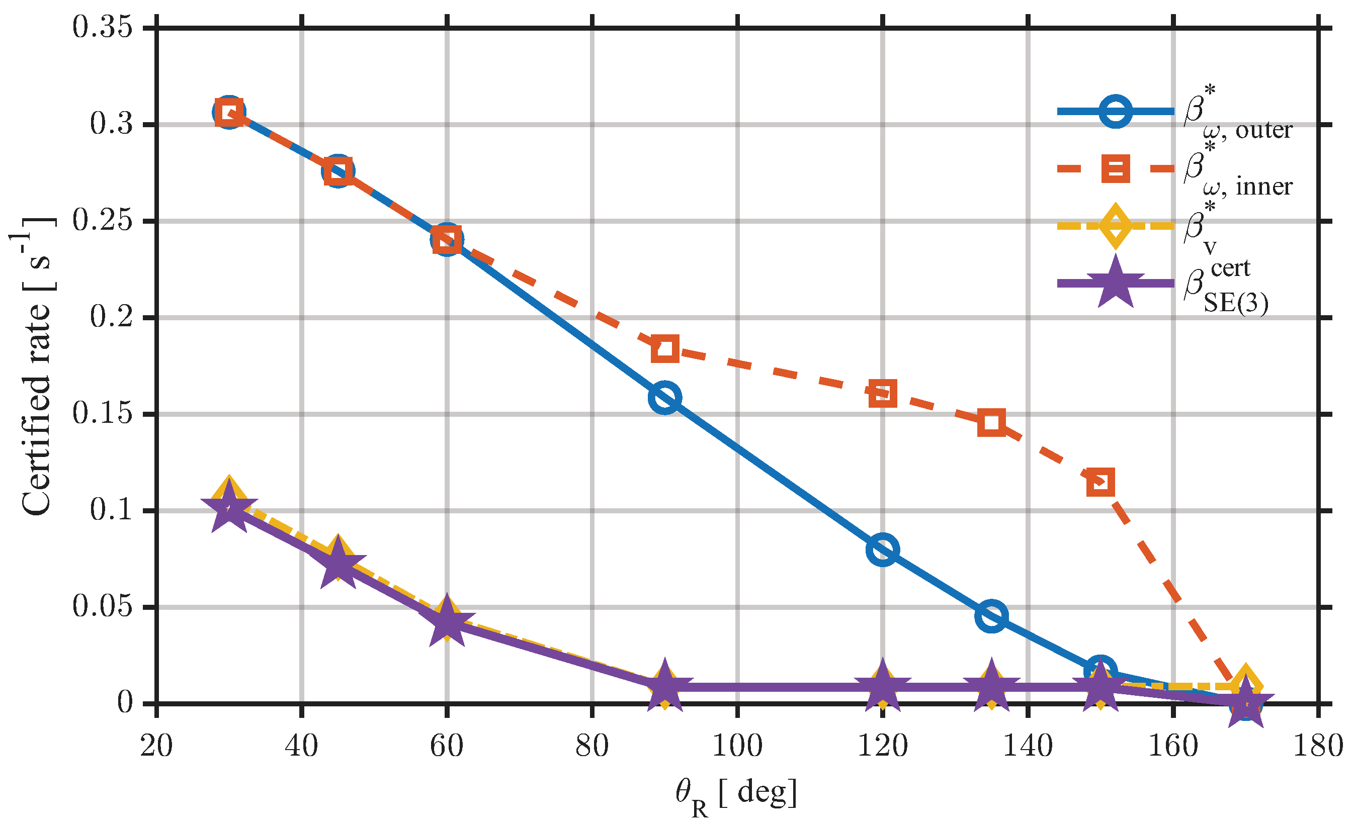
with 25 candidate values per dimension. The rate-bisection tolerance is ${10}^{-4}{\mathrm{s}}^{-1}$, the metric strictness margin is ${\epsilon }_g={10}^{-6}$, and the numerical SDP feasibility tolerance is ${10}^{-7}$. These are prescribed engineering search ranges, selected to span low- to high-gain responses while excluding values associated with excessive control authority; they are not mathematical limits of the controller. The reported gains are therefore grid-optimal within these finite search sets. The ${60}^{\circ }$ region contains the nominal ${55}^{\circ }$ case, the ${150}^{\circ }$ outer region contains the ${149}^{\circ }$ stress test, and the ${80}^{\circ }$ translational region is chosen below the ${90}^{\circ }$ limitation of the scalar-block translational metric. Figure 1 shows the expected rate–region trade-off: enlarging the admissible attitude region decreases the certified outer rotational rate, and the complete Phase-2 rate is limited by the translational subsystem over the feasible angle range. No positive ${170}^{\circ }$ rotational certificate is found in the tested gain grid and metric family.

Table 2. Angle-dependent grid-optimal gains and prescribed-region contraction rates.

${\mathit{\theta }}_{\mathit{R}}$ [deg]	${\mathit{\theta }}_{\mathit{T}}$ [deg]	${\mathit{k}}_{\mathit{\omega }}^{*}$	${\mathit{k}}_{\mathit{v}}^{*}$	${\mathit{\beta }}_{\mathit{\omega },\mathbf{out}}^{*}$ [s−1]	${\mathit{\beta }}_{\mathit{v}}^{*}$ [s−1]	${\mathit{\beta }}_{\mathbf{SE}\left(3\right)}^{\mathbf{cert}}$ [s−1]	Bottleneck
170	80	N/C	$137.707$	N/C	$0.008972$	N/C	N/C
150	80	$31.5557$	$137.707$	$0.016541$	$0.008972$	$0.008524$	Translation
135	80	$23.7675$	$137.707$	$0.045288$	$0.008972$	$0.008524$	Translation
120	80	$20.6271$	$137.707$	$0.079773$	$0.008972$	$0.008524$	Translation
90	80	$15.5362$	$137.707$	$0.158569$	$0.008972$	$0.008524$	Translation
60	60	$11.7017$	$247.462$	$0.240540$	$0.044312$	$0.042096$	Translation
45	45	$10.1556$	$312.845$	$0.276001$	$0.075897$	$0.072102$	Translation
30	30	$10.1556$	$351.754$	$0.306458$	$0.106476$	$0.101152$	Translation

N/C denotes “no certificate”, meaning that no positive prescribed-region certificate was obtained within the tested gain grid and metric family.

reports the corresponding angle-dependent grid-optimal designs. All rows use the same $25\times 25$ gain grids, the angular-momentum bound is $p_{\max }=2.10\mathrm{kg}{\mathrm{m}}^2/\mathrm{s}$, the reference angular-velocity bound is ${\omega }_{\max }^{*}=0.05\mathrm{rad}/\mathrm{s}$, and the hierarchy margin is ${\gamma }_h=0.95$. The reported solutions are grid-optimal within the prescribed finite gain ranges. Since $k_R^{*}=65$ and $k_p^{*}=100$ for every feasible row, only the angle-dependent damping gains are listed.

Table 2 quantifies the rate–region trade-off shown in Figure 1. Enlarging the outer rotational region increases the selected rotational damping gain and reduces the certified outer rotational rate. No positive rotational certificate is obtained at ${\theta }_R={170}^{\circ }$ within the tested gain grid and metric family; this absence of a certificate does not imply instability. For all feasible rows, the complete Phase-2 rate is limited by the translational subsystem.

The complete multi-angle offline certification used to generate Figure 1 and Table 2 required $3.4375\times {10}^4$ s ($9.55$ h) of measured wall-clock time on a Windows 11 workstation equipped with an Intel Core Ultra 9 185H processor and 32 GB of memory. The computation used MATLAB R2026a Update 2, CVX 2.2, and SDPT3 4.0. This time includes the rotational and translational $25\times 25$ gain-grid searches and the bisection-based feasibility tests over all reported angle regions. The measured time is implementation-dependent, but the computation is performed only once offline; no SDP or LMI is solved during closed-loop operation.

The small-angle design uses

$$(k_R,k_{\omega },k_p,k_v)=(65,11.7017,100,247.462),$$

which gives ${\beta }_{\omega }^{*}=0.240540{\mathrm{s}}^{-1}$, ${\beta }_v^{*}=0.044312{\mathrm{s}}^{-1}$, and ${\beta }_{SE\left(3\right)}^{\mathrm{cert}}=0.042096{\mathrm{s}}^{-1}$. The large-angle design uses

$$(k_R,k_{\omega },k_p,k_v)=(65,31.5557,100,137.707).$$

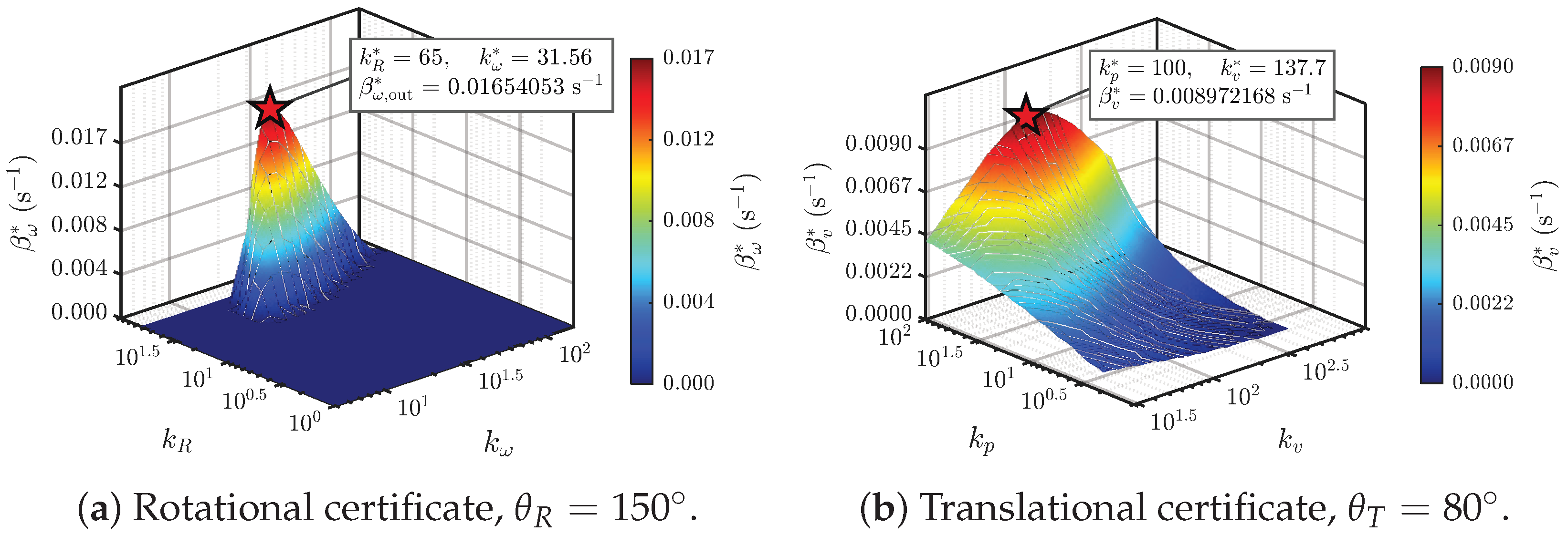
Its outer ${150}^{\circ }$ rotational rate is ${\beta }_{\omega ,\mathrm{out}}^{*}=0.016541{\mathrm{s}}^{-1}$; after entry into the inner ${80}^{\circ }$ region, the rotational rate increases to ${\beta }_{\omega ,\mathrm{in}}^{*}=0.114807{\mathrm{s}}^{-1}$. The corresponding translational and complete-cascade rates are ${\beta }_v^{*}=0.008972{\mathrm{s}}^{-1}$ and ${\beta }_{SE\left(3\right)}^{\mathrm{cert}}=0.008524{\mathrm{s}}^{-1}$. The associated large-angle rate surfaces are shown in Figure 2.

To examine this point directly,

Table 3. Effect of the rotational damping gain on the certified rotational rate at fixed $k_R=65$.

Certified Region	Gain Type	${\mathit{k}}_{\mathit{\omega }}$	${\mathit{\beta }}_{\mathit{\omega }}^{*}$ [s−1]
${60}^{\circ }$	Low damping	$5.0000$	$0.01740$
${60}^{\circ }$	Grid optimum	$11.7017$	$0.24054$
${60}^{\circ }$	Higher damping	$41.8960$	$0.10187$
${60}^{\circ }$	Very high damping	$150.0000$	$0.02380$
${150}^{\circ }$	Lower damping	$20.6270$	N/C
${150}^{\circ }$	Grid optimum	$31.5557$	$0.01654$
${150}^{\circ }$	Higher damping	$41.8960$	$0.01434$
${150}^{\circ }$	Very high damping	$150.0000$	N/C

compares representative rotational damping gains at fixed $k_R=65$. For both angle regions, the largest tested damping does not produce the largest certified rate. In the ${150}^{\circ }$ region, both insufficient and excessive damping can remove the positive regional certificate. Hence, the SDP is selecting a balance between dissipation, curvature, and the complete off-diagonal differential coupling, rather than merely selecting the largest damping coefficient.

Here, N/C means that no positive prescribed-region rate was certified at that grid point; it does not imply instability of a particular nominal trajectory. Table 3 verifies the numerical purpose of the gain search: within the tested grid, the selected damping gains maximise the certified rotational rate for their respective regions.

5.1.2. Small-Angle Scenario: $\theta \left(0\right)={55}^{\circ }$

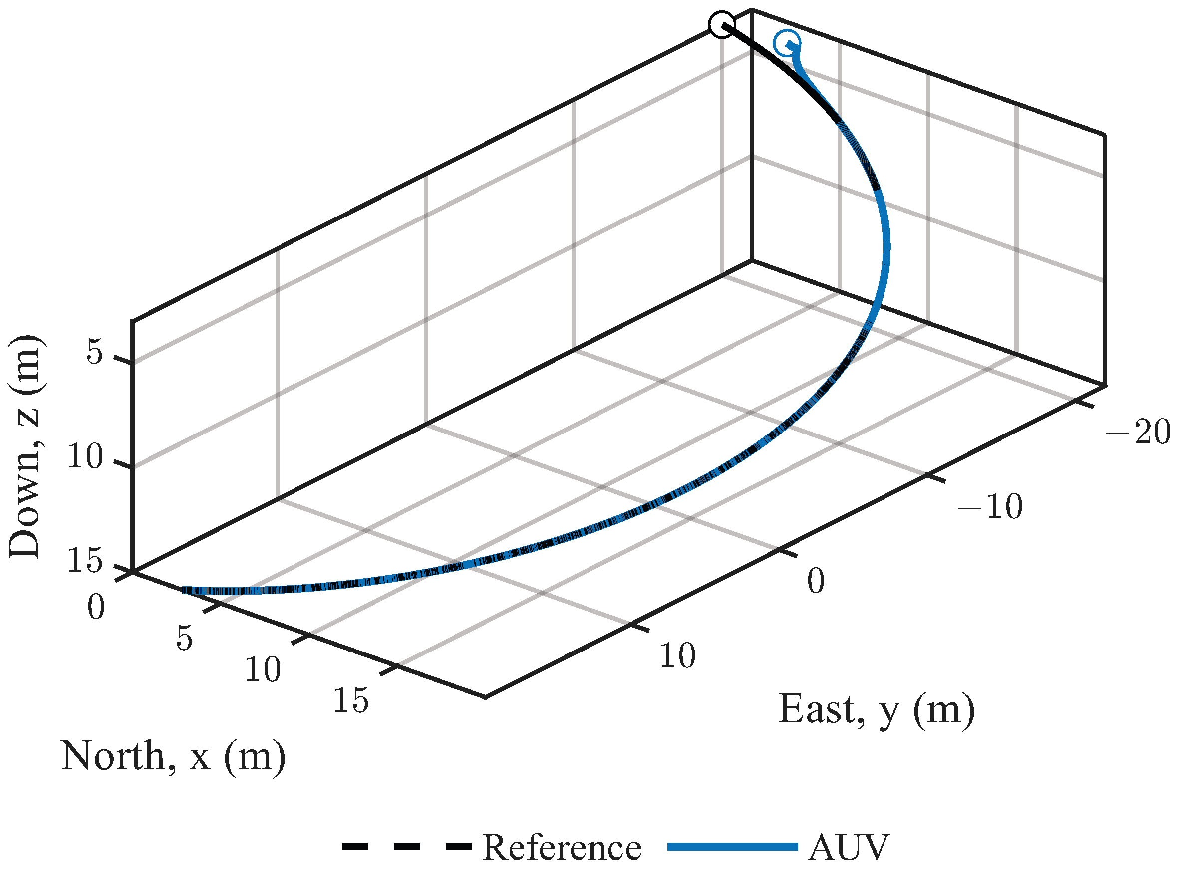
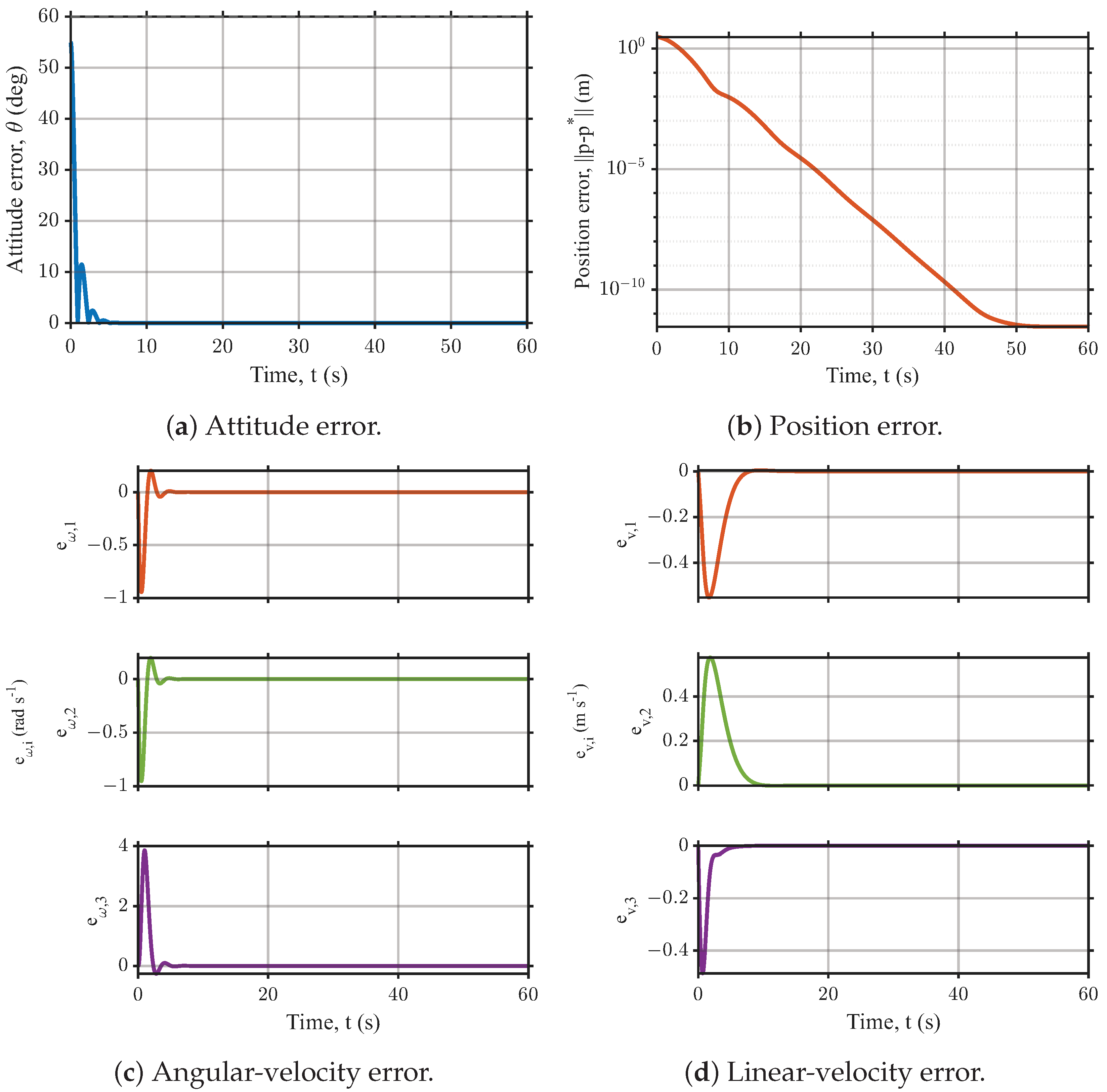
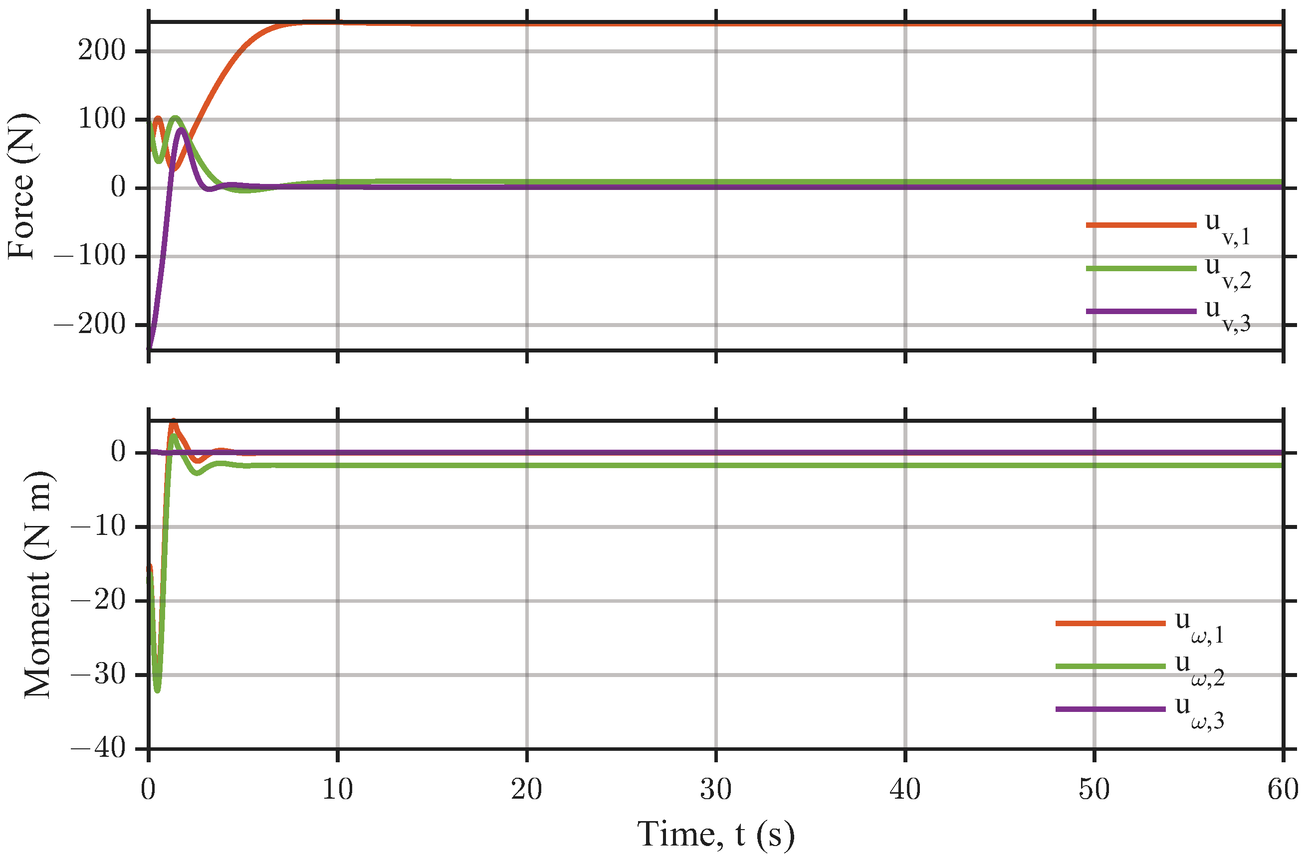
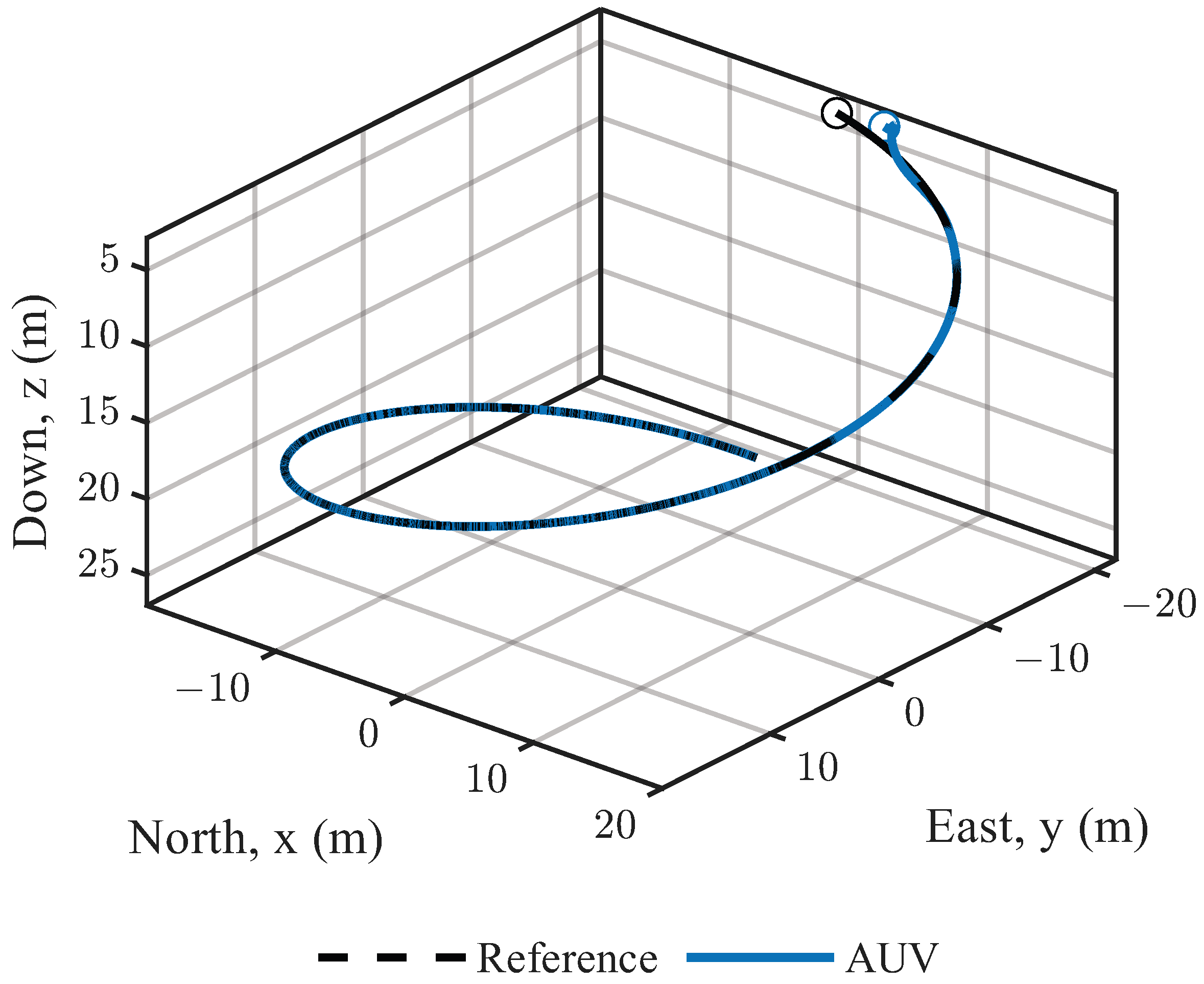
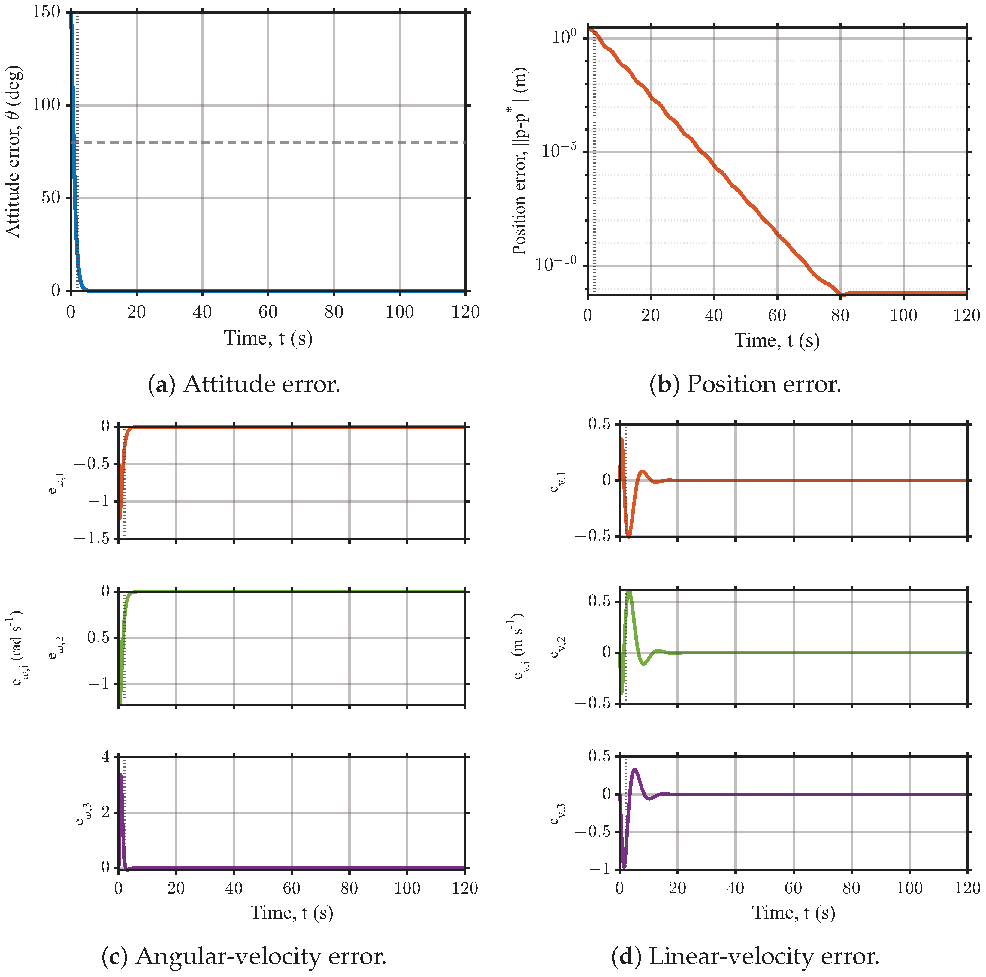
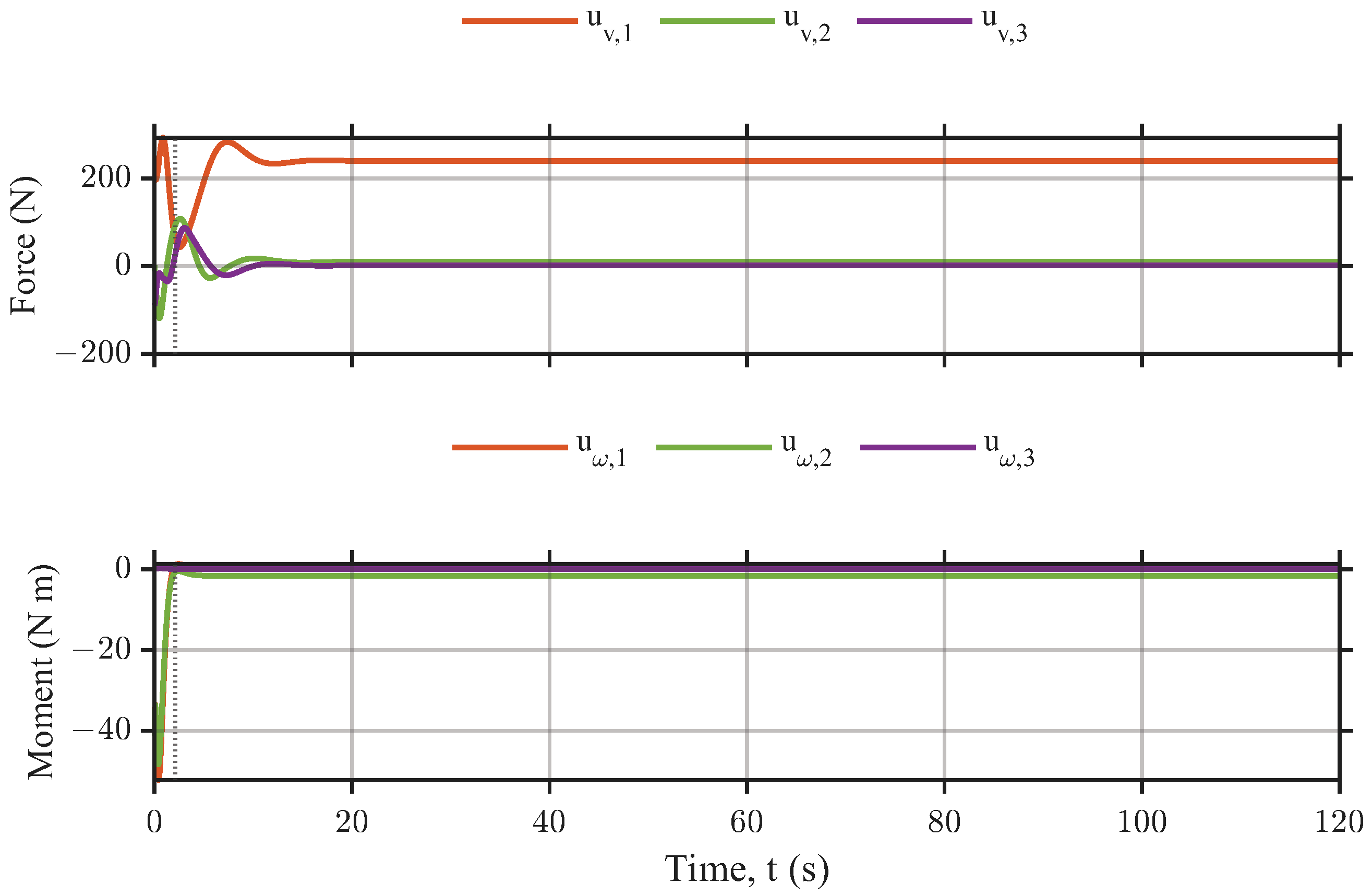
The initial attitude is obtained by rotating ${\mathbf{R}}^{*}\left(0\right)$ through ${55}^{\circ }$ about ${[1,1,0]}^{\top }/\sqrt{2}$, with initial position error ${[2,-2,1]}^{\top }$ m and zero transported momentum error. The three-dimensional trajectory in Figure 3 shows convergence to the helical reference. Figure 4 further shows decay of the attitude, position, angular-velocity, and linear-velocity errors, while Figure 5 reports the corresponding control force and moment. These plots verify the closed-loop implementation of the nominal DPSC dynamics; the contraction claim is assessed separately through the exact matrix audit below.

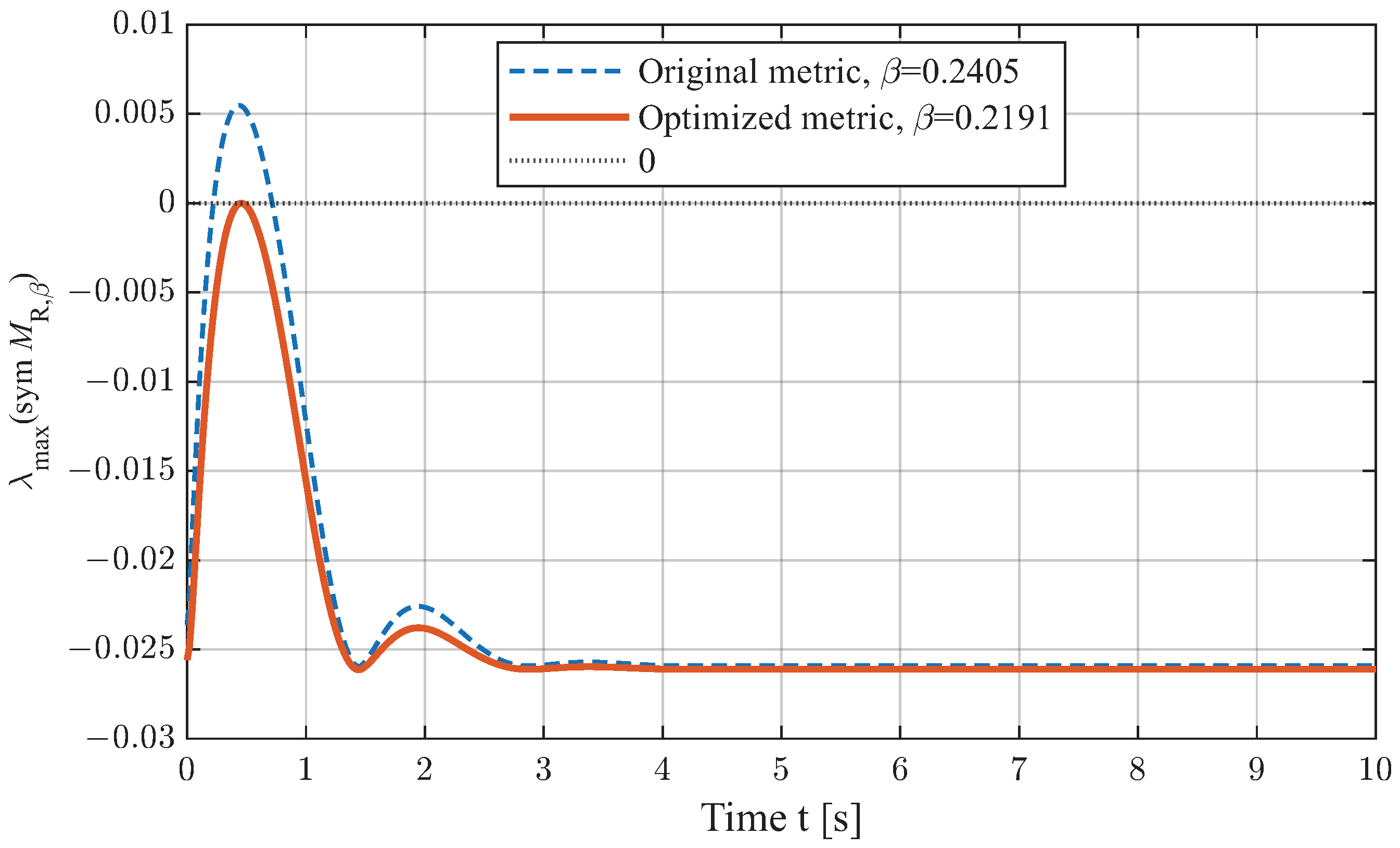
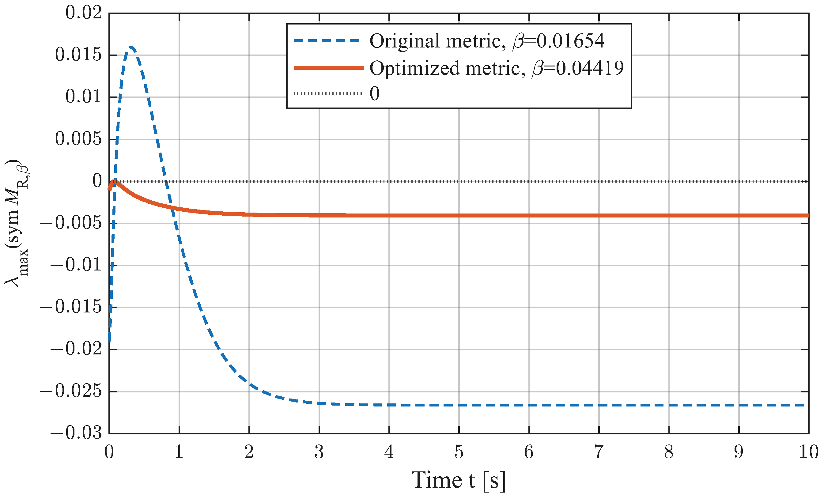
The realised angular momentum reaches $7.1804\mathrm{kg}{\mathrm{m}}^2/\mathrm{s}$ and therefore exceeds the conservative $p_{\max }=2.10\mathrm{kg}{\mathrm{m}}^2/\mathrm{s}$ used in the rectangular regional relaxation. Figure 6 compares the original regional metric at its grid-optimal rate with a single metric constrained to satisfy both the original regional SDP and all exact sampled-trajectory LMIs. The original metric at ${\beta }_{\omega }^{*}=0.240540{\mathrm{s}}^{-1}$ has a short positive excursion. The joint region–trajectory metric,

$$m_2=9.4959\times {10}^{-3},m_3=2.4725\times {10}^{-3},$$

keeps the exact matrix negative over the full sampled trajectory at ${\beta }_{\omega }=0.219116{\mathrm{s}}^{-1}$, with ${\max }_t{\mathrm{\Lambda }}_R(t;{\beta }_{\omega })=-1.77\times {10}^{-6}$. Since this rate remains well above ${\beta }_v^{*}$, the complete-cascade bottleneck remains the translational subsystem. This result verifies that one fixed metric can simultaneously satisfy the prescribed ${60}^{\circ }$ regional conditions and the exact realised small-angle trajectory.

5.1.3. Certificate-Aligned Large-Angle Scenario: $\theta \left(0\right)={118}^{\circ }$

This scenario was constructed without changing the large-angle controller gains, the original ${150}^{\circ }$ regional metric, or its reported rate. The initial attitude error is a ${118}^{\circ }$ rotation about ${\mathbf{e}}_2$, the initial angular momentum is zero, and the reference is smoothly started by the virtual-time map

$$\tau \left(t\right)={\int }_0^{t}s\left(\sigma \right)\mathrm{d}\sigma ,s\left(t\right)=\left\{\begin{array}{cc}10r^3-15r^4+6r^5,\hfill & 0\le t\le T_r,\hfill \\ 1,\hfill & t>T_r,\hfill \end{array}\right.r={\displaystyle \frac{t}{T_r}},T_r=2\mathrm{s}.$$

(83)

The realised angular momentum still reaches $7.7800\mathrm{kg}{\mathrm{m}}^2/\mathrm{s}$, so the purpose of this case is not to force the trajectory inside the conservative momentum rectangle. Instead, it tests whether a mission that is better aligned with the regional metric can retain the exact contraction inequality despite this norm excursion.

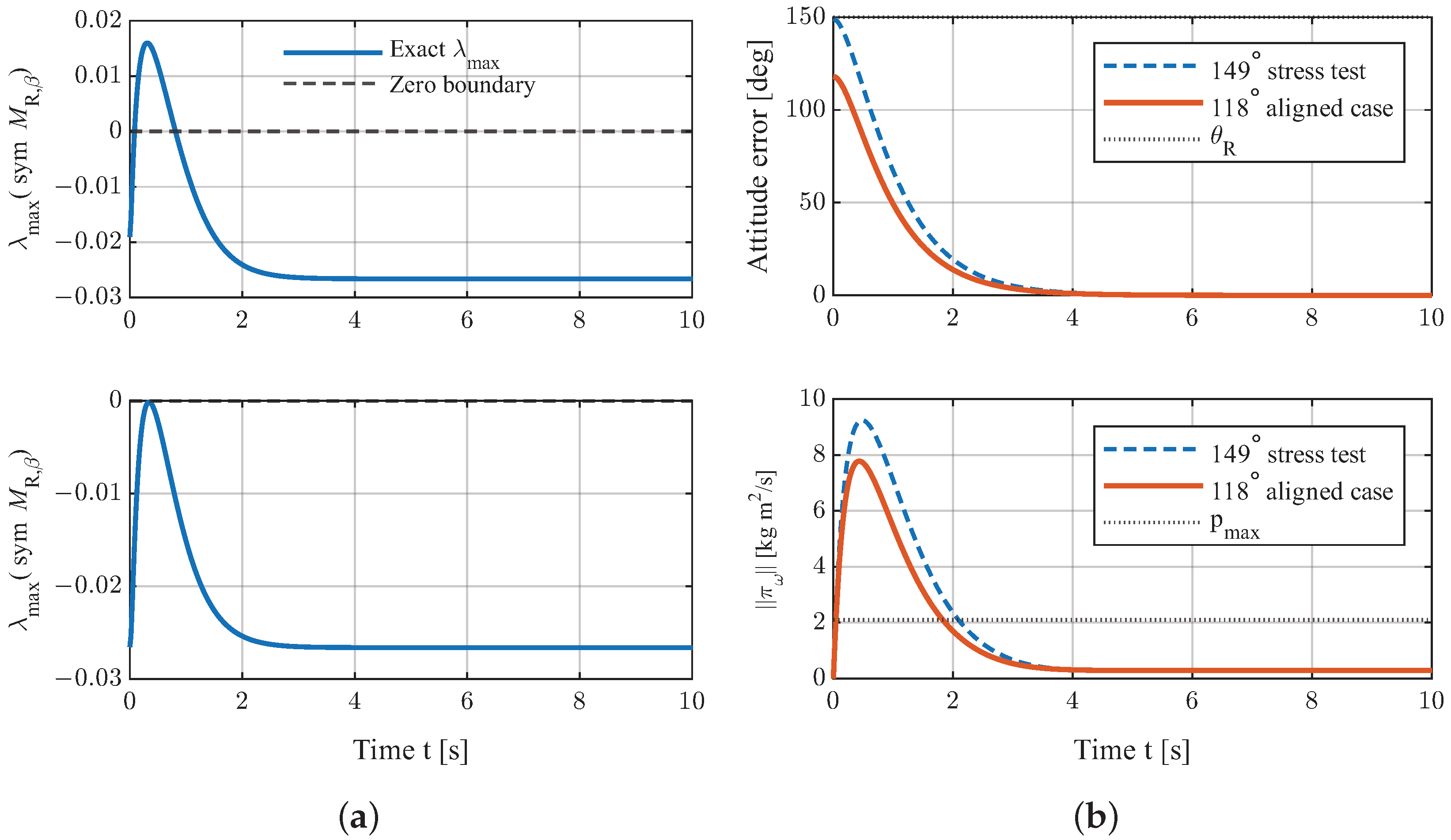
Figure 7 shows that the original regional metric at ${\beta }_{\omega ,\mathrm{out}}^{*}=0.0165405{\mathrm{s}}^{-1}$ remains strictly contracting along the complete sampled trajectory, with

$$\underset{t}{\max }{\mathrm{\Lambda }}_R(t;{\beta }_{\omega ,\mathrm{out}}^{*})=-1.3213\times {10}^{-4},\underset{t}{\max }{\mathrm{\Lambda }}_R(t;0)=-3.1629\times {10}^{-3}.$$

The result demonstrates that the conservative scalar momentum bound is not the exact boundary of contraction. The relative directions among the attitude error, angular momentum, angular velocity, and reference motion also determine the exact matrix.

5.1.4. Near-Antipodal Stress Test: $\theta \left(0\right)={149}^{\circ }$

The ${149}^{\circ }$ initial attitude error is generated at about ${[1,1,0]}^{\top }/\sqrt{2}$ and probes a manoeuvre close to the excluded ${180}^{\circ }$ attitude set. Figure 8, Figure 9 and Figure 10 show that the same fixed controller tracks the helical reference without switching, while the attitude, position, and velocity errors converge after a larger transient. The trajectory enters and subsequently remains in the complete Phase-2 tube at approximately $t_0=2.10\mathrm{s}$, consistent with the energy-entry/Phase-2 structure of the large-angle theorem.

The angular-momentum peak is $9.2444\mathrm{kg}{\mathrm{m}}^2/\mathrm{s}$. Under the original regional metric, the exact rate-shifted matrix reaches ${\max }_t{\mathrm{\Lambda }}_R(t;0.0165405)=0.015985>0$ during the early transient; even the zero-rate matrix reaches $0.011033>0$. Thus, the original regional metric cannot certify the complete realised trajectory from $t=0$. However, keeping the controller gains fixed and optimising only one constant metric over the stored trajectory gives

$$m_2=5.7609\times {10}^{-3},m_3=1.6845\times {10}^{-4},{\beta }_{\omega ,\mathrm{traj}}=0.044189{\mathrm{s}}^{-1},$$

with ${\max }_t{\mathrm{\Lambda }}_R(t;{\beta }_{\omega ,\mathrm{traj}})=-3.37\times {10}^{-7}$. Figure 11 therefore distinguishes two complementary statements: the prescribed-region SDP supplies a uniform worst-case certificate, whereas the trajectory-conditioned search supplies a fixed-metric certificate for this particular nominal manoeuvre. The latter is not used to enlarge the uniform regional theorem.

Table 4. Trajectory-wise rotational contraction audit for the nominal scenarios.

Scenario	Fixed Metric	Audit Rate [s−1]	${\max }_{\mathit{t}}{\mathbf{\Lambda }}_{\mathit{R}}$	${\max }_{\mathit{t}}\parallel {\mathit{\pi }}_{\mathit{\omega }}\parallel$	Regional Condition	Trajectory Audit
${55}^{\circ }$	Joint region–trajectory	$0.219116$	$-1.77\times {10}^{-6}$	$7.1804$	Satisfied by the metric	Pass
${118}^{\circ }$	Certified ${150}^{\circ }$ regional	$0.0165405$	$-1.3213\times {10}^{-4}$	$7.7800$	Momentum bound exceeded	Pass
${149}^{\circ }$	Certified ${150}^{\circ }$ regional	$0.0165405$	$1.5985\times {10}^{-2}$	$9.2444$	Momentum bound exceeded	Fail during early transient
${149}^{\circ }$	Trajectory-conditioned	$0.044189$	$-3.37\times {10}^{-7}$	$9.2444$	Not a regional certificate	Pass

collects only the quantities that are directly relevant to the contraction audit. Tracking RMSE and settling-time comparisons are intentionally not included here; such performance indices are more informative when controllers or non-ideal operating conditions are compared under common test conditions.

The three scenarios serve distinct but complementary purposes. The ${55}^{\circ }$ case verifies that a single fixed metric can satisfy both the prescribed small-angle region and the exact realised trajectory. The ${118}^{\circ }$ case shows that the original large-angle regional metric can remain strictly contracting along a suitably aligned large-angle mission even when the conservative scalar momentum bound is exceeded. The ${149}^{\circ }$ case demonstrates the need for the energy-entry/Phase-2 theorem and reveals the distinction between region-oriented and trajectory-conditioned metric optimisation. Together with the gain-rate comparison, these results verify the numerical implementation and scope of the analytical certificates derived in Section 4.2.

5.2. Comparison of Contraction-Certified and Simulation-Tuned Gain Selection

For the quadratic desired dissipation potential considered here, the nominal DPSC law has the same computed-torque geometric-PD feedback form when identical gains and reference-transport terms are used. The purpose of this comparison is therefore to evaluate two gain-selection procedures rather than two fundamentally different pointwise controllers. The proposed design selects gains by maximising a prescribed-region contraction-rate certificate. The geometric-PD baseline uses the same model compensation, geometric errors, reference transport, and gain ranges, but its four gains are selected independently by a trajectory-specific simulation search without using any contraction condition in the tuning objective.

The comparison uses the nominal ${55}^{\circ }$ scenario. The geometric-PD search first minimises the normalised rotational tracking objective

$$J_R={\displaystyle \frac{1}{T}}{\int }_0^T{\left({\displaystyle \frac{\theta \left(t\right)}{\theta \left(0\right)}}\right)}^2\mathrm{d}t,J_p={\displaystyle \frac{1}{T}}{\int }_0^T{\left({\displaystyle \frac{\parallel \mathbf{p}\left(t\right)-{\mathbf{p}}^{*}\left(t\right)\parallel }{\parallel \mathbf{p}\left(0\right)-{\mathbf{p}}^{*}\left(0\right)\parallel }}\right)}^2\mathrm{d}t,$$

(84)

using a $9\times 9$ coarse grid followed by a local $9\times 9$ refinement for each subsystem. The rotational gains are selected from $J_R$, after which the translational gains are selected from $J_p$. To prevent improved tracking from being obtained merely through larger peak inputs, the geometric-PD candidates are constrained to peak force and moment limits equal to $105\%$ of those generated by the certified design. The resulting gains are

$${(k_R,k_{\omega },k_p,k_v)}_{\mathrm{cert}}=(65,11.7017,100,247.4616),$$

and

$${(k_R,k_{\omega },k_p,k_v)}_{\mathrm{GPD}}=(65,13.0140,100,174.0912).$$

Both solutions are grid-optimal only with respect to their stated objectives and finite search ranges.

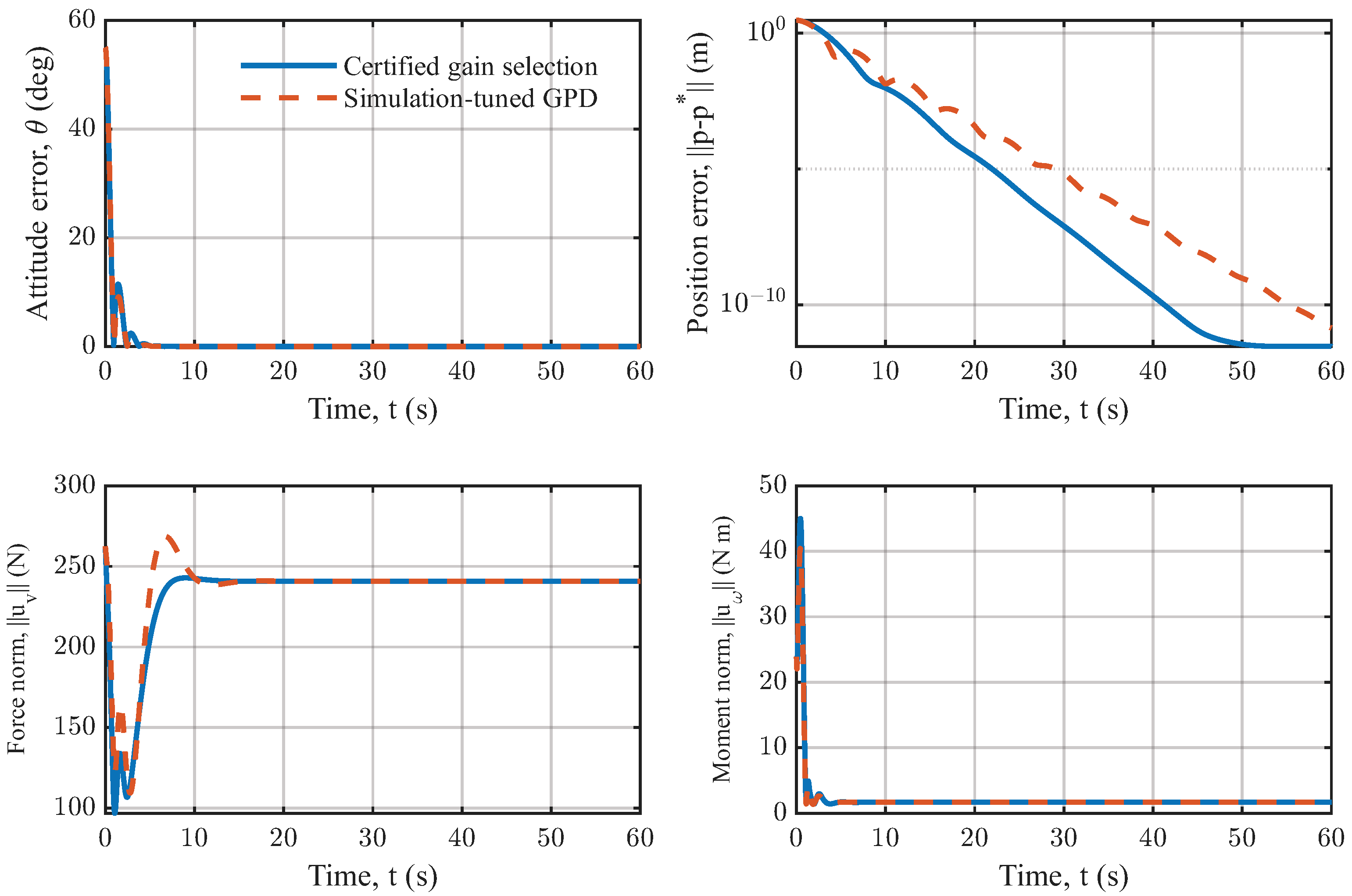
Figure 12 compares the resulting tracking-error and control-input histories, while

Table 5. Comparison of contraction-certified and independently simulation-tuned gain selection in the nominal ${55}^{\circ }$ scenario.

Gain-Selection Method	${\mathit{\beta }}_{\mathbf{SE}\left(3\right)}^{\mathbf{cert}}$ [s−1]	Att. RMSE [deg]	Pos. RMSE [m]	${\mathit{t}}_{\mathit{R}}$ [s]	${\mathit{t}}_{\mathit{p}}$ [s]	${\mathit{J}}_{\mathit{F}}$ [106 N2s]	${\mathit{J}}_{\mathit{M}}$ [103 (N m)2s]
Contraction-certified	$0.042096$	$4.5789$	$0.5117$	$3.46$	$6.98$	$3.2976$	$1.2332$
Simulation-tuned geometric PD	$0.039400$	$4.5657$	$0.4825$	$3.38$	$8.82$	$3.3707$	$1.0346$

reports the most relevant certificate and performance measures. Here, $t_R$ is the first time after which the attitude error remains below $1^{\circ }$, and $t_p$ is the first time after which the position error remains below $0.05$ m. The control-effort indices are

$$J_F={\int }_0^T\parallel {\mathbf{u}}_v{\left(t\right)\parallel }^2\mathrm{d}t,J_M={\int }_0^T{\parallel {\mathbf{u}}_{\omega }\left(t\right)\parallel }^2\mathrm{d}t.$$

The trajectory-specific geometric-PD tuning yields slightly lower attitude and position RMSE and a lower rotational control effort in this selected nominal manoeuvre. The contraction-certified design instead provides a $6.8\%$ larger complete prescribed-region rate certificate, a $20.9\%$ shorter position settling time, and a slightly lower translational control effort. An a posteriori application of the same certification procedure confirms that the simulation-tuned gains also admit a positive regional certificate, but with the smaller rate shown in Table 5. These results illustrate the difference between trajectory-specific performance tuning and region-oriented certified gain selection, rather than uniform superiority of one nominal feedback structure.

The peak force and moment were $262.44$ N and $45.00$ N m for the certified design and $268.60$ N and $40.42$ N m for the simulation-tuned design. Since both implementations use the same nominal pointwise feedback structure, the relevant additional computational burden of the proposed framework is the one-time offline SDP/LMI certification reported in Section 5.1.

5.3. Contraction-Oriented Robustness Under Non-Ideal Conditions

The nominal contraction certificates in Section 4.2 are derived for the exact ODIN model and therefore do not constitute a robust contraction theorem. This subsection instead provides a contraction-oriented numerical assessment of how representative model uncertainty, external disturbances, and measurement noise affect the incremental convergence observed in the certified ${55}^{\circ }$ tracking scenario. The reference trajectory, controller structure, and controller gains are kept unchanged in all cases.

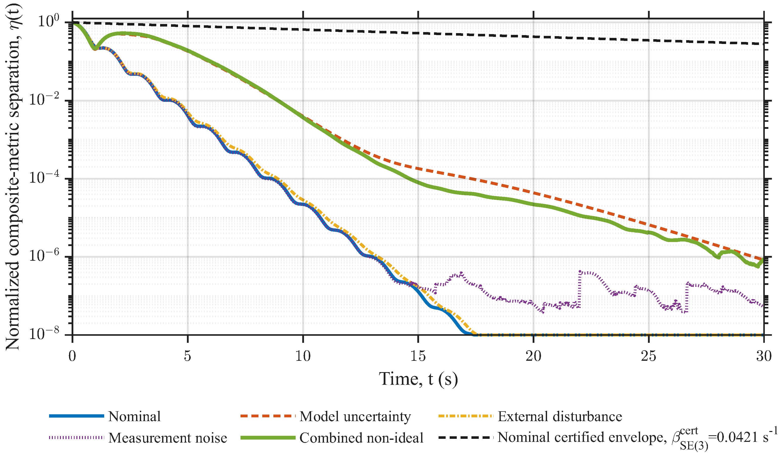
Five configurations are considered: the nominal model, model uncertainty only, external disturbance only, measurement noise only, and the combined non-ideal case. For the uncertainty-only case, the three principal translational inertias are scaled by $(1.15,0.90,1.08)$, the rotational inertias by $(1.12,0.92,1.08)$, the quadratic translational-drag coefficients by $(1.20,0.85,1.10)$, and the quadratic rotational-drag coefficients by $(0.90,1.15,1.20)$. The controller continues to use the nominal parameters. The external body-fixed force and moment have peak norms equal to $5\%$ and $10\%$, respectively, of the nominal peak control force and moment in the same manoeuvre. The measurement-noise signals are deterministic band-limited realisations with per-axis RMS levels of $0.02$ m in position, $0.{20}^{\circ }$ in attitude, $0.01$ m/s in linear velocity, and $0.005$ rad/s in angular velocity.

For each configuration, two neighbouring initial conditions are propagated under the same closed-loop dynamics and the same realisation of the exogenous signals. Their separation is evaluated using the nominal composite contraction metric,

$$d_{\mathcal{G}}\left(t\right)={\left(V_R\left(t\right)+\kappa V_v\left(t\right)\right)}^{1/2},\eta \left(t\right)={\displaystyle \frac{d_{\mathcal{G}}\left(t\right)}{d_{\mathcal{G}}\left(0\right)}}.$$

(85)

An empirical incremental decay rate ${\widehat{\beta }}_{\mathrm{inc}}$ is obtained by fitting $log\eta \left(t\right)$ over the interval $0.5\le t\le 15$ s, before the normalised separation reaches the prescribed numerical floor. This fitted quantity characterises the selected trajectory pair and signal realisation; it is not interpreted as a uniform robust contraction rate.

Figure 13 compares the normalised composite-metric separations with the nominal certified reference envelope. All tested cases retain an overall decay of the neighbouring-trajectory separation, although model uncertainty and the combined non-ideal condition introduce a pronounced non-monotone transient before the separation decreases to the numerical floor. The fitted rates and coefficients of determination in

Table 6. Contraction-oriented robustness summary for the ${55}^{\circ }$ scenario.

Case	${\widehat{\mathit{\beta }}}_{\mathbf{inc}}$ [s−1]	${\mathit{R}}^2$	Att. RMS [deg]	Pos. RMS [m]
Nominal	$1.0598$	$0.998$	$0.000$	$0.0000$
Model uncertainty	$0.6378$	$0.963$	$0.801$	$0.4751$
External disturbance	$1.0292$	$0.999$	$5.191$	$0.0619$
Measurement noise	$1.0612$	$0.998$	$0.199$	$0.0135$
Combined non-ideal	$0.6776$	$0.958$	$3.875$	$0.4551$

quantify this trajectory-wise trend. The black dashed curve is shown only as the nominal certified reference envelope; it is not a theoretical upper bound for the non-ideal trajectories.

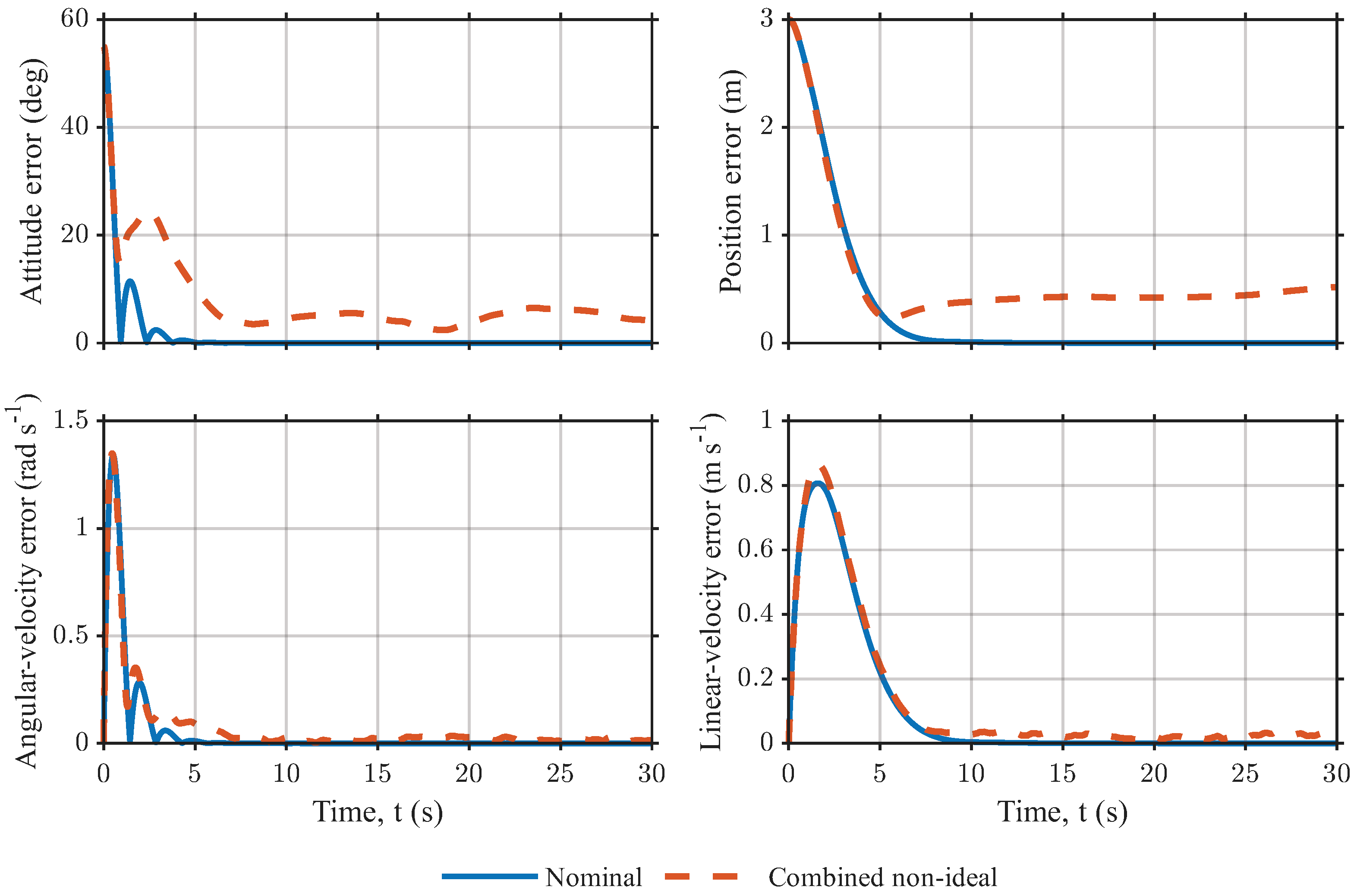
The composite separation describes incremental convergence between neighbouring trajectories and should be distinguished from convergence to the nominal reference. Figure 14 therefore compares the physical tracking errors of the nominal and combined non-ideal cases. The nominal errors converge to zero, whereas the combined case exhibits bounded, time-varying attitude, position, and velocity residuals under persistent uncertainty, disturbance, and noise. Consequently, the numerical results indicate that the incremental convergence tendency remains useful in the tested non-ideal realisation, but they do not imply zero tracking error or establish a robust contraction certificate for the perturbed plant.

6. Conclusions

This paper developed a contraction-certified trajectory-tracking and gain-selection framework for fully actuated AUVs on $SE\left(3\right)$. The AUV dynamics were represented in port-Hamiltonian form with a Rayleigh-type dissipation potential, and a dual potential shaping controller was used to construct an energy-structured closed loop with a rotational–translational cascade structure. For the quadratic desired dissipation potential considered in this work, the nominal feedback is algebraically equivalent to computed-torque geometric PD under identical gains and reference transport. The main contribution is therefore the regional contraction analysis and the associated offline gain certification for the complete AUV tracking cascade.

The rotational subsystem was analysed in fixed left-trivialised momentum coordinates using a cross-coupled differential metric. The resulting certificate retains anisotropic-inertia effects and the complete off-diagonal differential coupling. For the translational subsystem, a certified attitude-cover SDP was established for a general known symmetric positive-definite inertia matrix, while isotropic translational inertia admits a smaller exact endpoint formulation. The two subsystem certificates were combined through a scaled composite metric, proving every strict complete-cascade contraction rate below the slower subsystem rate. Large initial attitude errors were treated through a two-phase result: an energy argument first establishes sustained entry into the prescribed contraction tube, after which the complete cascade contracts without any change in the controller.

The four-gain certification problem was decomposed into two independent two-dimensional offline searches. The resulting procedure determines the controller gains, metric parameters, and certified rates for prescribed attitude, momentum, and reference-rate bounds, thereby providing a quantitative region–gain–rate relation. Numerical studies on the ODIN AUV obtained complete-cascade rates of $0.042096{\mathrm{s}}^{-1}$ and $0.008524{\mathrm{s}}^{-1}$ for the ${60}^{\circ }/{60}^{\circ }$ and ${150}^{\circ }/{80}^{\circ }$ rotational–translational regions, respectively. Small-angle, certificate-aligned large-angle, and near-antipodal manoeuvres illustrated the scope and conservatism of the regional certificates. Comparison with independently simulation-tuned geometric-PD gains further distinguished region-oriented certification from trajectory-specific performance tuning, without indicating uniform superiority of either gain-selection objective. Simulations with model variation, external disturbances, and measurement noise provided additional empirical evidence under non-ideal conditions, but were not interpreted as a robust contraction certificate or experimental validation.

The present framework is limited by the finite certified operating region, the conservatism of the sufficient differential bounds, and the assumption of exact nominal-model compensation. Future work will focus on incorporating actuator constraints directly into the contraction-based gain synthesis and evaluating the resulting controller on an experimental AUV platform under realistic hydrodynamic uncertainty.

References

1. Van Der Schaft, A.; Jeltsema, D. Port-Hamiltonian Systems Theory: An Introductory Overview. Found. Trends Syst. Control 2014, 1, 173–378. [Google Scholar] [CrossRef]
2. Ortega, R.; Van Der Schaft, A.; Maschke, B.; Escobar, G. Interconnection and Damping Assignment Passivity-Based Control of Port-Controlled Hamiltonian Systems. Automatica 2002, 38, 585–596. [Google Scholar] [CrossRef]
3. Guerrero-Sánchez, M.E.; Hernández-González, O.; Valencia-Palomo, G.; Mercado-Ravell, D.A.; López-Estrada, F.R.; Hoyo-Montaño, J.A. Robust IDA-PBC for Under-Actuated Systems with Inertia Matrix Dependent of the Unactuated Coordinates: Application to a UAV Carrying a Load. Nonlinear Dyn. 2021, 105, 3225–3238. [Google Scholar] [CrossRef]
4. Guerrero-Sánchez, M.E.; Montoya-Morales, J.R.; Valencia-Palomo, G.; Hernández-González, O. Robust IDA-PBC for Non-Separable PCH Systems under Time-Varying External Disturbances. Nonlinear Dyn. 2025, 113, 3499–3510. [Google Scholar]
5. Cisneros, R.; Fang, L.; He, W.; Ortega, R. A New Partial State-Feedback IDA-PBC for Two-Dimensional Nonlinear Systems: Application to Power Converters with Experimental Results. arXiv 2025, arXiv:2510.01425. [Google Scholar]
6. Donaire, A.; Perez, T. Dynamic Positioning of Marine Craft Using a Port-Hamiltonian Framework. Automatica 2012, 48, 851–856. [Google Scholar] [CrossRef]
7. Desai, R.P.; Manjarekar, N.S. Interconnection and Damping Assignment Passivity-Based Control for Dynamic Steering Position Stabilization of an Underactuated AUV. Adv. Control Appl. Eng. Ind. Syst. 2024, 6, e225. [Google Scholar] [CrossRef]
8. Fujimoto, K.; Sakurama, K.; Sugie, T. Trajectory Tracking Control of Port-Controlled Hamiltonian Systems via Generalized Canonical Transformations. Automatica 2003, 39, 2059–2069. [Google Scholar] [CrossRef]
9. Donaire, A.; Romero, J.G.; Perez, T. Trajectory Tracking Passivity-Based Control for Marine Vehicles Subject to Disturbances. J. Frankl. Inst. 2017, 354, 2167–2182. [Google Scholar] [CrossRef]
10. Donaire, A.; Romero, J.G.; Perez, T. Passivity-Based Trajectory-Tracking for Marine Craft with Disturbance Rejection. IFAC-PapersOnLine 2015, 48, 19–24. [Google Scholar] [CrossRef]
11. Lv, C.; Yu, H.; Chen, J.; Zhao, N.; Chi, J. Trajectory Tracking Control for Unmanned Surface Vessel with Input Saturation and Disturbances via Robust State Error IDA-PBC Approach. J. Frankl. Inst. 2022, 359, 1899–1924. [Google Scholar] [CrossRef]
12. Bullo, F.; Murray, R.M. Tracking for Fully Actuated Mechanical Systems: A Geometric Framework. Automatica 1999, 35, 17–34. [Google Scholar] [CrossRef]
13. Sanyal, A.; Nordkvist, N.; Chyba, M. An Almost Global Tracking Control Scheme for Maneuverable Autonomous Vehicles and Its Discretization. IEEE Trans. Autom. Control 2010, 56, 457–462. [Google Scholar]
14. Maithripala, D.H.S.; Berg, J.M. An Intrinsic PID Controller for Mechanical Systems on Lie Groups. Automatica 2015, 54, 189–200. [Google Scholar] [CrossRef]
15. Liao, Y.; Yan, X.; An, K.; Wang, Z.; Zhang, T.; Wu, S.; Jiang, D. Fixed-Time Geometric Tracking Control of Autonomous Underwater Vehicles on SE(3). Ocean Eng. 2024, 311, 118757. [Google Scholar] [CrossRef]
16. Yaghmaei, A.; Yazdanpanah, M.J. Trajectory Tracking for a Class of Contractive Port Hamiltonian Systems. Automatica 2017, 83, 331–336. [Google Scholar] [CrossRef]
17. Barabanov, N.; Ortega, R.; Pyrkin, A. On Contraction of Time-Varying Port-Hamiltonian Systems. Syst. Control Lett. 2019, 133, 104545. [Google Scholar] [CrossRef]
18. Yaghmaei, A.; Yazdanpanah, M.J. On Contractive Port-Hamiltonian Systems with State-Modulated Interconnection and Damping Matrices. IEEE Trans. Autom. Control 2023, 69, 622–628. [Google Scholar] [CrossRef]
19. Manchester, I.R.; Slotine, J.-J.E. Control Contraction Metrics: Convex and Intrinsic Criteria for Nonlinear Feedback Design. IEEE Trans. Autom. Control 2017, 62, 3046–3053. [Google Scholar] [CrossRef]
20. Wu, D.; Yi, B.; Manchester, I.R. Control Contraction Metrics on Lie Groups. arXiv 2024, arXiv:2403.15264. [Google Scholar]
21. Vang, B.; Tron, R. Geometric Attitude Control via Contraction on Manifolds with Automatic Gain Selection. In 2019 IEEE 58th Conference on Decision and Control (CDC); IEEE: New York, NY, USA, 2019; pp. 6138–6145. [Google Scholar]
22. Vang, B.; Tron, R. Global Attitude Control via Contraction on Manifolds with Reference Trajectory and Optimization. In 2020 59th IEEE Conference on Decision and Control (CDC); IEEE: New York, NY, USA, 2020; pp. 2006–2013. [Google Scholar]
23. Yaghmaei, A.; Yazdanpanah, M.J. Trajectory Tracking of a Class of Port Hamiltonian Systems Using Timed IDA-PBC Technique. In 2015 54th IEEE Conference on Decision and Control (CDC); IEEE: New York, NY, USA, 2015; pp. 5037–5042. [Google Scholar]
24. Lohmiller, W.; Slotine, J.-J.E. On Contraction Analysis for Non-Linear Systems. Automatica 1998, 34, 683–696. [Google Scholar] [CrossRef]
25. Simpson-Porco, J.W.; Bullo, F. Contraction Theory on Riemannian Manifolds. Syst. Control Lett. 2014, 65, 74–80. [Google Scholar] [CrossRef]
26. Slotine, J.-J.E. Modular Stability Tools for Distributed Computation and Control. Int. J. Adapt. Control Signal Process. 2003, 17, 397–416. [Google Scholar] [CrossRef]
27. Fossen, T.I. Handbook of Marine Craft Hydrodynamics and Motion Control; John Wiley & Sons: Hoboken, NJ, USA, 2011. [Google Scholar]
28. Duong, T.; Altawaitan, A.; Stanley, J.; Atanasov, N. Port-Hamiltonian Neural ODE Networks on Lie Groups for Robot Dynamics Learning and Control. IEEE Trans. Robot. 2024, 40, 3695–3715. [Google Scholar] [CrossRef]
29. Lee, T. Exponential Stability of an Attitude Tracking Control System on SO(3) for Large-Angle Rotational Maneuvers. Syst. Control Lett. 2012, 61, 231–237. [Google Scholar] [CrossRef]
30. Vang, B.; Tron, R. Non-Natural Metrics on the Tangent Bundle. arXiv 2018, arXiv:1809.06895. [Google Scholar]
31. Grant, M.; Boyd, S. CVX: Matlab Software for Disciplined Convex Programming, version 2.1; CVX Research, Inc.: Austin, TX, USA, 2014. [Google Scholar]
32. Lee, J.M. Introduction to Riemannian Manifolds, 2nd ed.; Springer: Cham, Switzerland, 2018. [Google Scholar]
Figure 1. Certified rate–region trade-off obtained from the offline 25 × 25 gain searches. A larger certified attitude region is obtained at the cost of a lower certified contraction rate.
Jmse 14 01465 g001
Figure 2. Certified-rate surfaces for the large-angle design. The selected gains are maxima of non-trivial rate landscapes rather than values obtained by monotonically increasing the damping gains. The stars indicate the selected grid-optimal gain pairs.
Jmse 14 01465 g002
Figure 3. Three-dimensional trajectory in the 55 small-angle scenario.
Jmse 14 01465 g003
Figure 4. Configuration and velocity tracking errors in the 55 scenario.
Jmse 14 01465 g004
Figure 5. Control force and moment in the 55 scenario.
Jmse 14 01465 g005
Figure 6. Largest eigenvalue of the exact rate-shifted rotational contraction matrix in the 55 scenario. The joint region–trajectory metric preserves strict negativity over the sampled trajectory, whereas the original regional metric at the slightly larger grid-optimal rate has a short positive excursion.
Jmse 14 01465 g006
Figure 7. Comparison of the 149 stress test and the certificate-aligned 118 scenario. The controller gains and the certified 150 regional metric are unchanged; only the initial-error direction and reference start-up are modified. (a) Exact contraction-matrix comparison. (b) Attitude and angular-momentum evolution.
Jmse 14 01465 g007
Figure 8. Three-dimensional trajectory in the 149 near-antipodal stress test.
Jmse 14 01465 g008
Figure 9. Configuration and velocity tracking errors in the 149 stress test. The horizontal dashed line in (a) marks the 80 Phase-2 tube boundary, and the vertical dotted lines indicate the sustained entry time t 0 .
Jmse 14 01465 g009
Figure 10. Control force and moment in the 149 stress test. The vertical dotted lines indicate the sustained entry time t 0 into the complete Phase-2 contraction tube.
Jmse 14 01465 g010
Figure 11. Largest eigenvalue of the exact rate-shifted rotational contraction matrix in the 149 stress test. The original regional metric loses negativity briefly, whereas a fixed trajectory-conditioned metric remains negative over the complete sampled trajectory.
Jmse 14 01465 g011
Figure 12. Nominal 55 tracking comparison between the contraction-certified gain selection and the independently simulation-tuned geometric-PD gain selection. The figure compares attitude error, position error, control-force norm, and control-moment norm.
Jmse 14 01465 g012
Figure 13. Normalised composite-metric separation under individual and combined non-ideal conditions. The black dashed curve denotes the nominal certified reference envelope.
Jmse 14 01465 g013
Figure 14. Tracking-error comparison between the nominal and combined non-ideal cases.
Jmse 14 01465 g014