Separating Sensor-like Anomalies from Regional Oceanographic Events: A Machine-Learning-Assisted, Physics-Guided, Event-Preserving Quality-Control Framework for Coastal Buoy Temperature Records

Abstract

Coastal upwelling and typhoon-driven mixing can cool a buoy record by several degrees within hours. Sensor faults do the same. Quality-control schemes that flag anomalies by residual magnitude alone therefore risk discarding real events. We analysed 30 min temperature records from six buoys and three depths off the east coast of Korea, spanning 2008–2024, and built a machine-learning-assisted, physics-guided, event-preserving quality-control framework that adds new labels without altering any observation or existing flag. Cooling events were catalogued from changes in the observed surface temperature and in the surface-to-bottom temperature difference and classified using three physically interpretable axes: spatial coherence with neighbouring buoys, vertical consistency between layers, and atmospheric forcing from ERA5 and typhoon best-track data. A station-wise ridge prediction model, fitted to the surface layer at five of the six stations, supplied prediction residuals that served only to flag candidates. Residual magnitude separated sensor-like anomalies from regional-event candidates poorly (direction-free AUC 0.52–0.56); upwelling-candidate and typhoon-related events produced residuals as large as those of the sensor-like reference group, or larger. The physical axes showed much stronger internal operational separability, reaching pairwise AUC values up to 1.000 and a multivariate cross-validated mean AUC of 0.987. These values do not represent external validation because the groups were partly defined using the same axes. The framework preserved regional-event candidates while affecting derived monthly means by at most about 0.0005 °C, yet retained event-scale cooling of up to about 8 °C. Prediction residuals are therefore useful for broad anomaly-candidate detection but insufficient for final event classification, which should rely on physically interpretable, multi-station criteria.

1. Introduction

Coastal high-frequency moored buoys integrate physical and biogeochemical sensors and provide real-time, two-way communication and sampling intervals as short as one minute, making them observing platforms capable of directly capturing short-term coastal phenomena such as current variability, typhoon passages, and internal waves [1,2,3]. Such real-time observations are combined with satellite data and numerical models to serve as foundational data for operational oceanographic systems that support coastal prediction and marine-disaster response [4,5,6]. Coastal temperature observations and sea surface temperature (SST) prediction products are further linked to short-term prediction and advisory systems for anomalous water temperatures, including high-water-temperature events [7,8,9,10]. In Korea, the National Institute of Fisheries Science established water-temperature advisory criteria in 2017, under which a summer high-water-temperature advisory is issued at a water temperature of 28 °C; the advisory was in force for 64 days in 2022 and 57 days in 2023 [11]. Over the thirteen years to 2023, natural disasters caused aquaculture losses of KRW 326 billion in Korean waters, of which high water temperature accounted for 60%, and the annual mean sea surface temperature in Korean waters rose by 1.44 °C over the 56 years to 2023 [11]. Reliable observation and interpretation of short-term temperature variability, including both abrupt warming and cooling, is therefore essential for coastal buoy temperature records.

The high scientific and operational value of these data makes reliable quality control (QC) a prerequisite for their use. The QARTOD manual specifies 13 real-time QC tests for stationary temperature–salinity sensors within a three-tier hierarchy, ranging from required timing/gap, syntax, location, gross range, and climatology tests to strongly recommended spike, rate-of-change, and flat-line tests and suggested multivariate, neighbour, and density inversion checks [12,13,14,15]. Even so, spurious measurements from ocean sensors are inevitable, and manual QC by experts is inefficient for large datasets and vulnerable to inconsistencies among reviewers; automatic QC is therefore essential for large, real-time data streams [16,17,18]. Prolonged marine exposure, biofouling, communication failures, sensor drift, and data gaps further underscore this need.

Nevertheless, traditional automatic QC procedures can produce high false-positive rates, partly because independent threshold-based tests often lack sufficient contextual awareness; in contrast, a multidimensional anomaly-detection approach has been shown to reduce classification error by at least 50% in hydrographic-profile QC [16,17,18]. In particular, for observations with strong seasonality and high intrinsic variability, univariate outlier detection based on quartiles or Z-scores has been shown to fail in identifying outliers distributed within the seasonal component [19,20,21]. This indicates that automatic QC can detect departures from a normal range, but cannot determine whether abrupt temperature changes in coastal records reflect sensor-related artefacts or real oceanographic phenomena.

To address these limitations, machine-learning-based QC has advanced in recent years. An intelligent QC method combining a transformer encoder with BiLSTM has been applied to marine buoy data for gap imputation and anomaly detection in an integrated manner [22], drawing on a broader body of work on deep learning for time-series anomaly detection [23,24]. A semi-supervised QC framework based on a GRU mean-teacher architecture [25], which adapts the mean-teacher scheme of Tarvainen and Valpola [26], noted that conventional QC relying on fixed thresholds and empirical rules struggles to accommodate diverse marine environments; related approaches have been applied to water-quality sensor networks [27]. A common premise in machine-learning anomaly detection is to learn the behaviour of good or normal data and to identify departures from it as outliers [16,17,18]. Recent machine-learning signal-processing work has also emphasised the need to avoid distorting genuine oceanographic features during anomaly removal, although such approaches remain primarily focused on anomaly reconstruction or denoising rather than event classification [28,29,30]. Even so, the magnitude of prediction residuals or reconstruction errors alone cannot distinguish sensor-like anomalies from physically plausible regional events. Recent work in ocean and coastal machine learning has emphasised interpretability and domain-informed feature construction. For significant wave height prediction, a physically motivated wave-height ratio combined with SHAP-based attribution has been shown to improve both skill and transparency [31]; for bathymetric mapping, spatially aware feature engineering and adaptive normalisation have been used to address spatial autocorrelation across contrasting seabed terrains [32]. These approaches have not, however, been adapted to quality control, where distinguishing a sensor artefact from a dynamic oceanographic event requires multi-station spatial coherence, vertical consistency and physical forcing constraints rather than feature attribution alone. In other words, previous studies have concentrated on improving anomaly-detection performance, gap imputation, and automatic flagging, but have not sufficiently provided physically interpretable criteria for separating sensor-like anomalies from physically plausible regional-event candidates in multi-station, multi-layer coastal temperature records.

Meanwhile, abrupt cooling observed in coastal waters may be a real oceanographic phenomenon rather than noise to be removed. The western coastal waters of the East Sea (Japan Sea), along the east coast of Korea (hereafter, WES), form a dynamically variable marginal-sea region influenced by interactions between warm-current systems, including the East Korea Warm Current (EKWC), and cold coastal waters [33,34,35]. In summer, southerly or southwesterly winds can induce coastal upwelling along parts of the Korean east coast, bringing cold subsurface water toward the surface; in the southwestern East Sea, this process is further modulated by alongshore currents, stratification, and topography [36,37,38]. Along the southern coast of Korea, upwelling has been reported to persist for more than a month after upwelling-favourable winds weakened, with coastal SSTs about 2 °C below the climatological mean, while offshore waters were about 2 °C warmer than normal, producing an unusually strong coastal–offshore temperature contrast and seriously affecting fishing grounds [39,40,41]. During typhoon passages, vertical mixing and Ekman upwelling cause rapid surface cooling, with in situ observations showing cooling of up to about 8 °C and cold wakes persisting for days to weeks [42,43,44]; such cooling is explained by upper-ocean physical responses, including entrainment, vertical mixing, and upwelling [45,46,47]. Single-point surface observations alone are insufficient to resolve the vertical structure of these responses [48,49,50]. It should be noted, however, that the case regions of these previous studies do not fully coincide with the buoy stations examined here; these references are therefore understood not as direct validation for specific stations, but as evidence that regional cooling events are physically plausible phenomena in the WES. Accordingly, the regional-event labels used in this study should be interpreted as physically supported candidates rather than independently confirmed upwelling events.

Building on this problem, the present study develops and evaluates an event-preserving QC framework using multi-station, multi-layer coastal buoy temperature records from the WES, comprising six stations and three depth layers sampled at 30 min intervals from 2008 to 2024, corresponding to more than five million nominal station-layer records before accounting for gaps. In this framework, AI prediction residuals are treated as evidence of statistical unexpectedness rather than as evidence of sensor malfunction, and spatial coherence, vertical consistency, and physical forcing are combined to separate sensor-like anomalies from regional-event candidates. Because this approach uses multi-station spatial coherence as a discriminant axis without relying solely on external reference SST products, it provides an alternative discriminant axis that can mitigate dynamic-area overscreening in reference-based QC [51,52,53,54]. The framework is not intended to replace conventional QC, but to add an event-aware interpretive layer that supports the review and preservation of physically plausible coastal temperature events. Application of the framework shows that the magnitude and sign of prediction residuals alone did not separate sensor-like anomalies from regional-event candidates (univariate discrimination AUC 0.52–0.56), whereas a multivariate discrimination combining spatial coherence, southerly-wind forcing, and vertical consistency achieved high separability (cross-validated AUC 0.987, an internal operational separability rather than external validation). As a result, the framework preserved event-scale cooling signals (median cooling amplitude of about 2.5 °C, up to about 8 °C) while leaving monthly mean temperatures essentially unchanged (maximum monthly mean change ≤ 0.0005 °C). The contributions of this study are threefold: first, it demonstrates that residual magnitude alone cannot separate sensor-like anomalies from physically plausible regional events; second, it presents discrimination criteria based on spatial–vertical–forcing consistency using a multi-station, multi-layer buoy array; and third, through an additive, flag-not-remove design that leaves the original values and existing QC flags unmodified, it preserves event-scale cooling signals without distorting long-term climatology. Thus, the framework acts primarily as an event-scale preservation tool rather than a climatological correction procedure.

2. Materials and Methods

2.1. Study Area, Buoy Observations, and Baseline QC

The primary data are coastal buoy temperature records maintained by the National Institute of Fisheries Science (NIFS) in the western coastal waters of the East Sea (Japan Sea), along the east coast of the Republic of Korea (hereafter, WES). Six stations were used —Gangneung (bgna3), Samcheok (bsc87), Yangyang (byy87), Yeongdeok (byd8a), Goseong-Bongpo (fgbg3) and Goseong-Gajin (fggo3); their locations are shown in Supplementary Figure S1. The two Goseong identifiers (fgbg3 and fggo3) correspond to the same physical location before and after a buoy replacement and are therefore treated as separate station identifiers with distinct records but identical coordinates. Each station reports temperature at three nominal vertical layers (surface, middle and bottom) at 30 min resolution. The records span 2008–2024; individual stations differ in their available periods, and the most recently deployed station (fggo3) has a short record beginning in 2024 (Table S1).

The data had previously been processed through two frozen QC stages (Phase 1 and Phase 2), whose outputs are the fields qc_temp2 and qcode_temp2. Only qc_temp2 follows the IOOS/QARTOD-like flag convention, in which good = 1, suspect = 3, fail = 4 and missing = 9; qcode_temp2 carries study-specific diagnostic subcodes that record which test was activated. Standard real-time QC of temperature observations comprises 13 tests within a three-tier hierarchy, ranging from required timing/gap, syntax, location, gross range and climatology tests to strongly recommended spike, rate-of-change and flat-line tests and suggested multivariate, neighbour and density inversion checks [12,13,14,15]. The complete Phase-1 and Phase-2 test list, the thresholds applied and the full qcode mapping are given in Table S7.

Across the integrated record of 2,973,722 rows, the frozen Phase-2 QC classified 2,964,082 observations (99.7%) as good and 9640 as suspect or fail. Most good observations carry no diagnostic subcode (qcode 1; 2,880,414 rows, 96.9%); a further 83,668 rows (2.8%) carry the stuck-release subcodes 12 and 13, which record that a Phase-1 stuck flag was re-examined in Phase 2 and released to good. Among the non-good rows, the rate-of-change test dominates (qcode 21; 7273 rows), followed by layer inversion (qcode 32; 754), spike (qcode 23; 683) and surface–bottom cross suspicion (qcode 41; 662). The Phase-3 codes 51–59 introduced in the present work are study-specific additive diagnostic codes and are not QARTOD codes; they are written to separate fields and never to qcode_temp2, which contains no value in the range 51–59 anywhere in the record. The main data components and additive AI-QC fields are summarised in

Table 1. Data sources and quality-control fields used in this study.

Component	Content	Role/Notes
NIFS buoy temperature	6 stations × 3 layers (surface/middle/bottom), 30 min, 2008–2024	Primary data; discrimination target and normal-state training
Stations	bgna3, bsc87, byy87, byd8a, fgbg3, fggo3	fggo3 short record (from 2024); surface-only AI applied to 5 stations
Frozen QC fields	qc_temp2 follows the IOOS/QARTOD-like flag convention (good 1, suspect 3, fail 4, missing 9); qcode_temp2 stores diagnostic subcodes	Phase-1/2 outputs; never overwritten
Atmospheric forcing (ERA5)	u10, v10, t2m, mslp, sp	Along-shore wind and storm alibi; inputs to M2 only
KMA marine buoy (Pohang)	Hourly wind, pressure, air temperature	Validation-only regional atmospheric alibi; ERA5 reliability check; not an AI input
Typhoon best-track	Storm centre time, position, central pressure	Independent typhoon support (gold typhoon; alibi for contamination screening)
AI-QC additive fields	ai_pred_residual, ai_error_z, ai_event_qcode (51–59), ai_event_label, preserve/restore masks, review level	Attached separately; values and Phase-2 flags unchanged

.

All times in this study are Korea Standard Time (KST, UTC+9). Event construction, event matching against the typhoon best-track, the figures and all reported dates follow this convention; ERA5 and best-track fields, which are distributed in UTC, were converted before use. The buoys are serviced on a monthly schedule, during which sensor operation is verified and the sensors are cleaned.

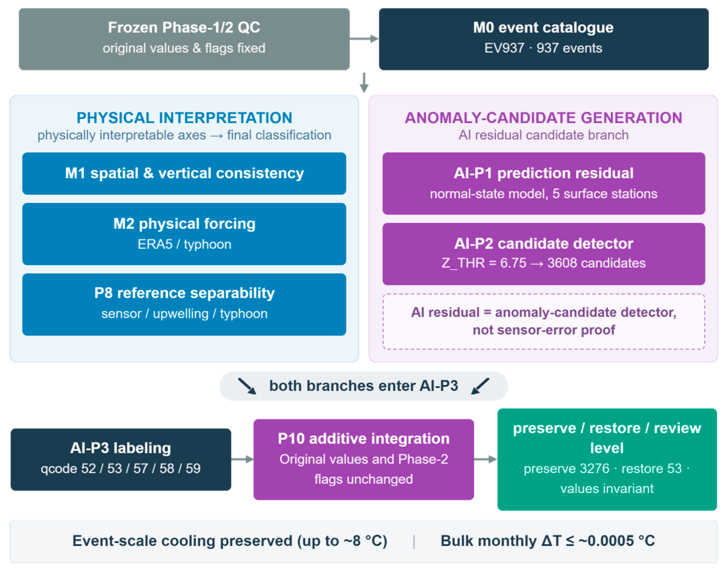
The present Phase-3 AI-QC does not overwrite these Phase-2 flags. Instead, it follows a flag-not-remove principle: every Phase-3 result is written to separate, additive fields, and no temperature value, qc_temp2 value or qcode_temp2 value is modified. This design keeps the QC record fully audit-traceable—each Phase-3 flag records which axes were activated—and lets a downstream user decide whether to include or exclude flagged events for a given analysis. It also embodies the framework’s central stance that the AI component is not the final judge: its outputs are candidate material and review priorities, not automatic failures. The overall workflow (Figure 1) comprises two streams: M0–M2 define physically interpretable event axes and reference/candidate groups, whereas AI-P1–P3 use prediction residuals to detect additional candidate events and assign additive review/preservation labels.

2.2. M0: Baseline Residual Decomposition and Event Catalogue

The M0 stage is a harmonic/statistical residual decomposition, not a deep-learning model. The decomposition was fitted separately for each station–layer channel using clean Phase-2 observations, defined by qc_temp2 = 1, qcode_temp2 not in {13, 41}, and finite temperature values. Temperature was separated into a slowly varying trend, an annual component and a monthly diurnal component, and a residual. The trend was estimated as a 13-month centred moving average of monthly means. Monthly means were computed from the clean observations with no minimum sample requirement, and the moving average was taken over a complete calendar-month axis on which months without observations were left missing and skipped; the window was shortened at the beginning and end of each record, and the smoothed monthly trend was interpolated linearly onto the full time axis and extrapolated at the two ends. The trend is separated but never removed automatically because long-term warming of the East Sea is itself a target of downstream analysis. The annual component was a first-order harmonic in sin/cos(2πd/365.25) with an intercept, and the diurnal component was a month-specific first-order harmonic in sin/cos(2πh/24). The requirement of at least 100 clean samples applies to this monthly diurnal fit and not to the monthly means used for the trend. The residual is the observation minus the sum of these components, and channel×month residual quantiles (p99.5/p99.9/p99.95; default p99.9) were tabulated as context-dependent references.

Because the harmonic order is a free choice, the decomposition was repeated with a second-order annual term, a second-order diurnal term, and both. The residual standard deviation changed by less than 0.5% and the residual 99.9th percentile by less than 0.3%, and the group medians of the minimum temperature residual, one of the discriminant axes used in Section 3.2, shifted by less than 0.1 °C. The event catalogue described below is unaffected by this choice because it is built from the observed temperature field rather than from the residuals.

A cooling–stratification-reduction event catalogue (EV937; 937 events) was then constructed. The catalogue is defined from changes in the observed temperature field, not from the harmonic residuals. Changes over 24, 48 and 72 h were computed for diagnostic comparison, and the 48 h scale was used for detection:

dT_surf = T_surf(t) − T_surf(t − 48 h)

(1)

dStrat = [T_surf − T_bottom](t) − [T_surf − T_bottom](t − 48 h)

(2)

dT_bottom = T_bottom(t) − T_bottom(t − 48 h)

(3)

These differences were evaluated where both the surface and the bottom record were Phase-2 good. Candidate points were those in the lower 10% tail of dT_surf combined with either the lower 10% tail of dStrat, giving the surface-stratification type, or the lower 10% tail of dT_bottom, giving the whole-column cooling type; the two types were pooled. Candidate points were merged into events using a 12 h merge gap and a 12 h minimum duration. Lowering the tail cut from 10% to 5%, 2.5% and 1% reduced the number of candidate points to 33%, 11% and 3% of the value at the adopted cut (44,230 points at 1 0%), as expected from the definition; the 10% cut is used throughout. M0 and this catalogue are thus a residual and event generator and a diagnostic baseline; they are not a final classifier.

2.3. M1: Spatial and Vertical Consistency Analysis

M1 evaluates whether an anomalous event is spatially coherent across neighbouring stations and whether it is vertically consistent between the surface and bottom layers. For each target station, the three nearest neighbours by haversine distance were selected (fggo3 was excluded as a predictor because it shares a location with fgbg3 and has a short record). The surface M0 residual was regressed on neighbour surface residuals by robust regression, and the standardised deviation z from this fit was mapped to categories: |z| < 2 spatially consistent, |z| ≥ 3 local anomaly, intermediate values mixed or ambiguous, and fewer than two valid neighbours insufficient. Intermediate cases were classified as mixed when spatially coherent and incoherent responses co-occurred within an event window, and as ambiguous when no dominant category reached the event-level assignment threshold (50% of an event’s points). Across EV937, the spatial categories were spatially consistent (552), mixed event (133), insufficient neighbours (130), ambiguous (86) and local anomaly (36). Vertical structure was summarised by refined flags: coherent cooling required a surface–bottom shape correlation of at least 0.36 and a timing lag within 15 h, whereas a high-frequency bottom ratio of at least 0.75 combined with a shape correlation below 0.2 flagged a bottom artefact; additional flags described weak bottom co-cooling, surface-only or decoupled responses, no bottom cooling and absence of a bottom record. Vertically coherent cooling, together with spatial coherence, supports a regional physical interpretation, whereas strong vertical inconsistency (for example, a surface-only or decoupled response) is consistent with a sensor-like artefact. M1 provides interpretable physical axes rather than an automatic fail decision.

2.4. M2: Physical-Forcing Interpretation

M2 is likewise not a deep-learning model. It uses ERA5 atmospheric-forcing variables [55] and typhoon best-track information to attach a physical interpretation label to each event. ERA5 hourly fields (u10, v10, t2m, mslp, sp; SST excluded) were restricted to a land–sea-masked box spanning 36.0–38.6° N and 128.3–130.2° E, and for each buoy station, a 30 km radius-weighted average over the sea grid cells within that box was used; all fields were referenced to KST. Along-shore wind was computed as u·sin(θ) + v·cos(θ), where θ is the coastline azimuth measured clockwise from north. A single value of θ = 0° was applied at all six stations, since the coast between Goseong and Yeongdeok runs approximately north–south; no station-specific azimuth was fitted. With this choice, the along-shore component is the meridional wind component v10, and positive values denote southerly, upwelling-favourable wind. Forcing was evaluated over the event window relative to a preceding 72 h background, and a southerly-forcing condition required a positive along-shore anomaly or a positive event-mean along-shore wind together with a same-month percentile of at least 60. Typhoon influence was derived from the RSMC Tokyo (JMA) best-track dataset (Japan Meteorological Agency, RSMC Tokyo-Typhoon Centre, Tokyo, Japan), referenced to UTC and converted to KST for buoy comparison; the closest point of approach (CPA) to each buoy region was computed as the nearest point on the great-circle track segments (haversine), with CPA time, central pressure and intensity obtained by linear interpolation along the segment. A CPA within 100 km was treated as strong direct typhoon influence, whereas a CPA within 300 km and ±3 days was used as a broader typhoon-influence screen. Following a circularity-avoidance principle, sea-surface temperature products (ERA5 SST and satellite SST) are not used as inputs or calibration labels, and only atmospheric variables enter the interpretation. A satellite-only level-3 product was examined for a small subset of events as a post hoc sanity check after the analysis was complete; it played no part in the framework and is reported separately in Section 4.6. Level-4 gap-free analyses were not used because they assimilate in situ observations and interpolate across cloud gaps, so they can neither serve as independent evidence nor distinguish a missing observation from the absence of a cold anomaly; their use in upwelling-dominated coastal settings has also been advised against on the basis of a direct comparison with in situ loggers [56]. M2 labels were assigned by applying these conditions in a fixed order. An event within the strong typhoon-influence radius was labelled typhoon-related; among the remainder, an event meeting the southerly-forcing condition was labelled upwelling-supported if it was also spatially coherent and upwelling-candidate otherwise; an event with cooling but without southerly forcing was labelled regional natural non-upwelling; an event whose forcing diagnostics were available but did not meet any of these conditions was labelled unresolved local-anomaly; and an event for which the forcing fields could not be evaluated was labelled insufficient-context. Across EV937, the most frequent M2 labels were upwelling_supported (292), regional_natural_nonupwelling (290), physical_forcing_unclear (121), and typhoon_mixed (77). The label strings reported in Section 3.1 are the machine-readable names produced by this rule set, and each maps to one of these five categories; where the forcing diagnostics were partly available but inconclusive, the event carries an explicit qualifier such as physical_forcing_unclear or mixed_unclear. An M2 label is an interpretation and protection label, not a failure decision.

2.5. External Verification of Atmospheric Forcing (Circularity Avoidance)

Because buoy-defined events must not be validated with the same buoy signals used to detect them, we cross-checked the ERA5 atmospheric forcing against an independent in situ record. This verifies the atmospheric fields that enter the interpretation; it does not test the identity of the events themselves. The reliability of the ERA5 atmospheric fields was validated against the Korea Meteorological Administration (KMA) Pohang marine buoy, which provides a long, continuous in situ record of the regional wind field, pressure and air temperature. Agreement was high for pressure and air temperature (mean sea-level pressure R² = 0.994, RMSE ≈ 0.60 hPa; 2 m air temperature R² = 0.956) and moderate-to-good for the wind components (wind speed R² = 0.74; zonal and meridional components R² ≈ 0.80; along-shore wind R² ≈ 0.77), based on approximately 1.2 × 10⁵ hourly matchups. The KMA Pohang buoy served as the primary reliability check because the ERA5 grid nearest Yeongdeok contains roughly 42% land. Therefore, the KMA Pohang buoy was used to evaluate whether ERA5 captured regional atmospheric variability relevant to event interpretation, not to validate temperature responses at individual NIFS stations, and it was never used as an AI training input.

The upwelling–wind link was tested independently with an event-level (one value per event) Wilcoxon signed-rank test to avoid pseudoreplication. Along-shore (southerly) wind during the 72 h preceding upwelling-candidate events, and during the events themselves, was significantly stronger than background (pre-72 h minus background median difference 1.91, p = 1.4 × 10⁻²¹, rank-biserial 0.66; event minus background 2.29, p = 3.7 × 10⁻²³, rank-biserial 0.70; n = 198), and the monthly event count correlated with along-shore wind (Spearman ρ = 0.67, p = 0.018). Hourly pooled tests were treated as supplementary because of pseudoreplication. For thirteen storms passing near the array, ERA5 and the KMA buoy agreed closely on the minimum pressure (median ERA5-minus-buoy difference 0.38 hPa, p = 0.54) while ERA5 underestimated the maximum wind speed relative to the buoy (median difference −5.65 m s⁻¹, p = 2.4 × 10⁻⁴). Sea-surface temperature products were not used as model inputs or calibration labels in order to avoid circularity with the buoy temperature target. The satellite comparison described in Section 4.6 was carried out after the analysis was complete and is presented as a sanity check rather than as validation.

2.6. Reference Groups and Separability Analysis

To evaluate the discriminant axes, we defined three reference and candidate groups from physically explicit criteria. Only the typhoon group is anchored outside the buoy signal, through the best-track record; the other two are defined from the array itself. The gold typhoon group (77 events) is supported by typhoon best-track information, independent of the buoy signal; it was defined at the station-event level when an EV937 event overlapped a typhoon influence window derived from best-track CPA (a 100 km CPA indicating strong direct influence and up to 300 km used as a broader typhoon screen) and the associated pressure and wind response, using a ±3-day window around the closest approach. The sensor-like reference group (17 events) is defined by the joint occurrence of spatial isolation, absence of physical forcing and vertical inconsistency. These criteria describe the absence of physical support rather than positive evidence of an instrument fault, so the group can be assembled from the buoy array without asserting what the buoy signal cannot establish. This does not, however, make the resulting separability measures independent: the same axes are used both to define the group and to discriminate it, and the values reported in Section 3.2 should be read accordingly (see the note to

Table 2. Pairwise separability of reference and candidate event groups.

Discriminant Axis	Sensor-like vs. Upwelling-Candidate	Sensor-like vs. Typhoon-Related	Upwelling-Candidate vs. Typhoon-Related
Spatial coherence (frac_consistent)	1.000	0.848	0.650
Southerly-wind forcing (along_wind_pctile)	1.000	0.851	0.634
Vertical coherence (vertical_shape_corr)	0.846	0.665	0.790
Minimum temperature residual (M0_min_resid)	0.774	0.687	0.535
Neighbour-extreme count	0.608	0.532	0.574

Notes. Values are direction-free AUC, computed as max(AUC, 1 − AUC), so that 0.5 denotes no separation regardless of the sign of the axis. The contrast between the sensor-like reference group and the upwelling strong candidate group is not independent: both groups are defined using the same axes that are used here to discriminate them, so the values of 1.000 in that column are partly tautological by construction. The sensor-like versus typhoon-related contrast is partly independent because the typhoon group is defined from RSMC Tokyo best-track data rather than from the buoy signal; the values in that column are substantially lower (0.848 and 0.851 for the two strongest axes). We do not read this difference as a quantitative estimate of the inflation, since the two contrasts also differ in the physical processes involved. All values in this table represent internal operational separability, not external validation of event identity (Section 4.6).

and Section 4.6). The upwelling strong candidate group (65 events) is defined by spatial coherence, southerly-wind forcing and vertically coherent cooling. Consistent with a strict circularity-avoidance stance, this group is not termed “gold upwelling”: asserting the presence of upwelling from the same buoy signals used to detect it would be circular, so its members remain strong candidates pending independent evidence such as satellite SST, a wind-stress index, chlorophyll or documented cases. For the same reason, we use the term sensor-like reference group rather than “confirmed sensor error”. The buoys are serviced monthly, when sensor operation is checked and the sensors are cleaned, but records that would link an individual servicing action to a specific station and time were not available to us, so no member of this group is independently verified as an instrument fault. In each pairwise comparison, the first-named group was taken as the positive class, and all AUC values are reported direction-free as max(AUC, 1 − AUC), so that 0.5 denotes no separation regardless of the sign of the axis.

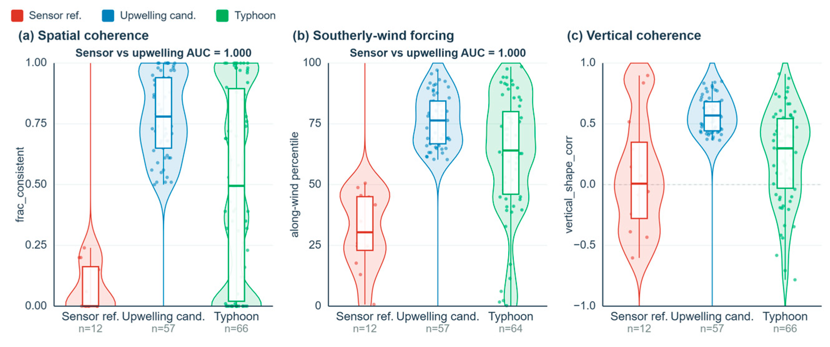
Separability was quantified in two distinct analyses whose provenance we keep explicit. First, single-axis, direction-free receiver-operating-characteristic (ROC) analysis [57] produced pairwise AUC values for each axis and each group pair (Section 3.2, Table 2). Second, a separate multivariate logistic classifier with 5-fold cross-validation combined the axes to estimate overall separability of sensor-like anomalies versus regional-event candidates; this cross-validation yielded a mean AUC of 0.987 and a pooled out-of-fold AUC of 0.981. Because the sensor-like and upwelling-candidate groups were defined partly by the same physical axes used for discrimination, the multivariate AUC should be interpreted as the internal separability of physically defined reference and candidate groups within the chosen discriminant space, rather than as independent validation of true event identity. The pairwise-AUC table and the multivariate cross-validation are different analyses and are reported separately throughout. The distributions of the discriminant axes for each group are shown in Figure 2.

2.7. AI-P1: Short-Term Prediction-Residual Model

AI-P1 is a short-term prediction-residual module in the spirit of predict-then-flag anomaly detection, deliberately simplified and used only as a candidate detector. Independent, station-wise models were built for the surface layer. Six surface stations were considered, but fggo3 was not modellable because its available surface record fell entirely within the test period, leaving no training data; five station models were therefore trained. For each station, predictors comprised five features per time step—the standardised temperature and the sine and cosine of hour-of-day and of day-of-year—stacked over the look-back window (48 steps for a 24 h look-back and 144 steps for a 72 h look-back at 30 min resolution). Four input/horizon combinations were evaluated, with look-back windows of 24 h and 72 h and prediction horizons of 1 h and 3 h, using a ridge-regression baseline [58]. Station-wise prediction errors for all input/horizon combinations are given in Table S2, and the cross-station summary is given in

Table 3. AI-P1 prediction performance and residual-only separability.

L/H	RMSE_Val (°C)	RMSE_Test (°C)	MAE_Test (°C)	Selected λ	AUC (Residual-Only)	Median |z| (Sensor/Upwelling/Typhoon)
L24H1	0.326	0.309	0.165	1–10	0.552	7.70/10.07/8.72
L24H3	0.528	0.507	0.294	—	0.541	4.63/7.17/5.65
L72H1	0.319	0.274	0.147	—	0.557	9.09/9.56/8.78
L72H3	0.514	0.457	0.263	—	0.518	5.52/6.91/5.76

Notes. RMSE_val is the validation-block error used for model selection; RMSE_test and MAE_test are held-out test errors. All three are unweighted means over the five modelled stations. The ridge penalty λ was selected independently at each station on the validation split from a grid spanning 10⁻⁴ to 10²; at the adopted configuration, the selected values were λ = 1 at three stations and λ = 10 at the other two. AUC values are direction-free separability of the standardised prediction residual between the sensor-like reference group and the regional-event candidates, computed at the event level.

. Cross-station means in both tables are unweighted averages over the five modelled stations, and held-out test errors are reported alongside the validation errors used for model selection: at the adopted configuration, the mean test RMSE was 0.309 °C and the mean test MAE 0.165 °C, against a validation RMSE of 0.326 °C. The selected ridge penalties were λ = 1 at three stations and λ = 10 at the other two, so no station required regularisation at either end of the search range. The ridge penalty was selected separately for each station and each look-back/horizon combination as the value minimising validation-block RMSE over a logarithmic grid (λ ∈ {10⁻⁴, 10⁻³, …, 10²}). Temperature was standardised using training-period statistics. Training, validation and test sets used a year-block split (train 2009–2021, validation 2022–2023, test 2024, adjusted by availability) rather than a random split; windows spanning a split boundary were purged. Clean training windows required qc_temp2 = 1, qcode_temp2 not in {13, 41}, finite input and target temperatures, and no overlap with excluded event windows—the sensor-like reference group, high-priority unresolved review events, gold typhoon windows, and upwelling strong candidate windows. The prediction target was raw surface water temperature; the output residual is the observed minus predicted temperature. Residuals were normalised by a robust, context-dependent scale σ_error computed as a station×layer×month median absolute deviation (with a fallback when monthly samples were sparse), giving a standardised error z. AI-P1 thus produced the additive fields ai_pred_residual, ai_error_z, ai_pred_status, ai_anomaly_flag and ai_point_qcode.

2.8. AI-P1 Model Selection and AI-P2 Residual-Candidate Detection

The look-back/horizon (L/H) combination was not selected on prediction error alone. Although the 72 h look-back with a 1 h horizon (L72H1) achieved a marginally lower cross-station RMSE than the 24 h look-back with a 1 h horizon (L24H1), the two combinations had essentially tied residual-only separability between sensor-like anomalies and regional-event candidates (direction-free AUC 0.557 versus 0.552, within the 0.01 tie tolerance), and L24H1 retained far greater usable event coverage (134 versus 78 reference events) while being the simpler, onset-sensitive configuration. L24H1 was therefore selected. We state this explicitly to avoid the misreading that the choice was driven by RMSE.

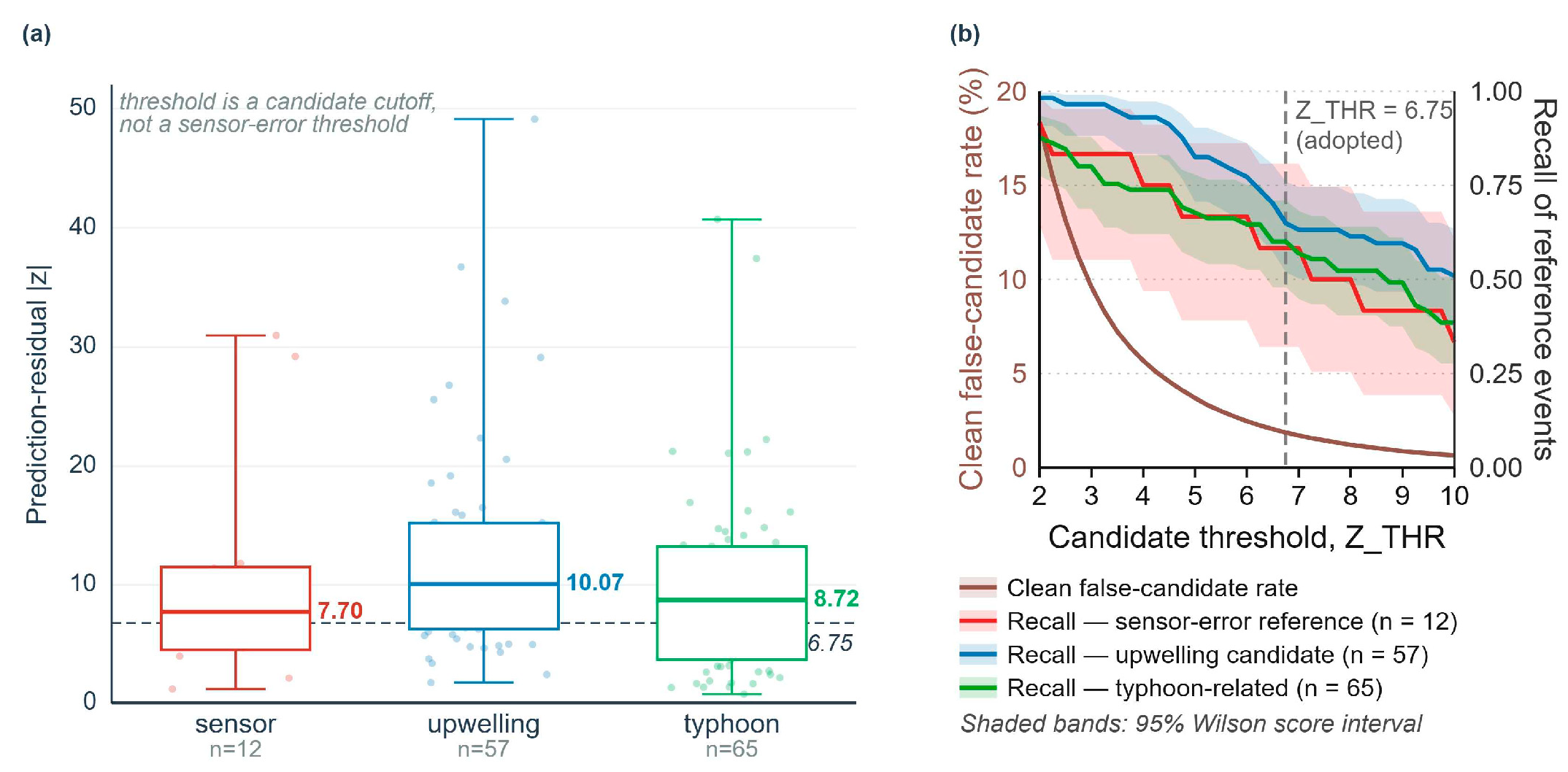
AI-P2 uses the prediction residual only to detect broad anomaly candidates. A candidate threshold of |ai_error_z| ≥ 6.75 was chosen as the value corresponding to a clean false-candidate rate of approximately 2% across stations (per-station 1.62–2.02%); the full candidate-threshold sensitivity is given in Table S3; this is a broad anomaly-candidate threshold, not a sensor-error threshold. Unless stated otherwise, the clean false-candidate rate is a point-level quantity computed over surface observations with a valid prediction residual, whereas recall and all qcode counts reported below are event-level quantities computed over merged candidate events. Candidate runs were consolidated with a merge gap of 2 steps and a minimum duration of 2 points, yielding 3608 candidate events (2305 spike-type and 1303 context-type); consolidated two-point runs were labelled spike-type, whereas runs longer than two points were labelled context-type. Of these, 713 overlapped the EV937 catalogue and 2895 were AI-only. A prediction-residual candidate is recorded with qcode 51, which denotes an anomaly candidate only and does not by itself indicate a sensor error. The candidate rate does not fall off sharply at any particular threshold, so the value adopted here reflects an operational judgement about review capacity rather than a statistical break: at 6.75, the 3608 candidate events correspond to about 91 per station-year of effective record, of which those routed to human review amount to about one per week.

2.9. AI-P3: Rule-Based Event Labelling

AI-P3 assigns event-level qcodes and labels to the AI-P2 candidates using the M1 spatial and vertical consistency, the M2 physical-forcing labels and the reference-group logic. It is rule-based, not supervised learning. The qcodes are 52 (vertical/layer inconsistency), 53 (spatial deviation), 57 (external-forcing mismatch or absence), 58 (possible regional event, preserved/review candidate) and 59 (human review, unresolved). qcode 58 is the key event-preservation flag; qcode 59 marks unresolved cases requiring human review. Reference-group priority is applied before general rule mapping: the sensor-like reference, gold typhoon and upwelling strong candidate logic take precedence, after which EV937-overlapping candidates inherit their catalogue interpretation and AI-only candidates receive a spatial co-occurrence triage. Importantly, AI-only candidates are not automatically classified as sensor errors; most are retained as high-review, unresolved cases unless adjacent-station co-occurrence supports a possible regional event.

2.10. Final Additive Integration

The integration stage (P10) attaches the AI-P2 point-level residual fields and the AI-P3 event-level labels to the original buoy table. Inputs were the frozen buoy_dorumuk6_qc2 record and the AI-P2 point and AI-P3 event products; outputs were the integrated record buoy_dorumuk6_qcAI_final together with point-level and event-level tables and an integration report. Joining used station, layer and time, with exact time matching applied first and a ±15 min nearest match allowed only when exact matching failed (the nearest time difference is recorded). Value invariance was verified: water_temp, qc_temp2 and qcode_temp2 were identical before and after integration. The preservation mask is defined as ai_event_qcode = 58, and the restore mask as ai_event_qcode = 58 together with a Phase-2 flag of suspect or fail and a finite temperature value; a review-priority field orders records as restore candidate > high review > mid review > preserve > none. AI prediction was applied to the five surface stations only; the middle and bottom layers and station fggo3 are marked not applicable.

3. Results

3.1. Characteristics of Flagged Anomaly Events in the Buoy Records

The cooling–stratification-reduction event catalogue EV937 comprised 937 events. Their M2 physical-forcing labels suggest that many of these catalogued cooling events carried physically interpretable or regional-event-like signatures rather than purely local, sensor-like characteristics. The most frequent labels were upwelling_supported (292), regional_natural_nonupwelling (290) and physical_forcing_unclear (121), followed by typhoon_mixed (77); the remaining events were distributed among insufficient_context (44), mixed_unclear (43), upwelling_possible_spatial_unresolved (37), localized_upwelling_candidate (20), unresolved_local_anomaly (12) and atmospheric_cooling_or_mixing (1). The M1 spatial categories tell a consistent story, with 552 of 937 events (59%) classified as spatially consistent. The convergence of these complementary descriptions—frequent spatial coherence and a predominance of upwelling-candidate or regional-forcing labels—suggests that a large fraction of the catalogued events were broad, physically structured candidates rather than isolated single-station excursions. We therefore describe them as regional-event-like or physically interpretable rather than as confirmed upwelling, since independent confirmation is not available for every event.

It is useful to ask how the frozen Phase-2 QC, which is a conventional threshold-based scheme, has already treated these events. At the event level, 18 of the 77 typhoon reference events (23.4%) and 13 of the 65 upwelling strong candidates (20.0%) contained at least one surface observation flagged as suspect or fail; across the full EV937 catalogue, the figure was 169 of 937 (18.0%). At the point level, these flags accounted for 1.29%, 0.85% and 1.01% of surface observations inside the corresponding event windows, against 0.265% over all surface observations, an enrichment of 3.2 to 4.9 times. Almost all of the flags originated from the rate-of-change test, which is the test a rapid cooling event is most likely to trigger. Conventional QC therefore does not remove these events wholesale, but it does flag them at several times the background rate, and the flags fall preferentially on the steepest part of the cooling—the part that carries the physical signal.

3.2. Separability of Sensor-like Anomalies and Regional-Event Candidates

Physically interpretable axes separated the reference groups far better than minimum temperature residual alone, although this separation is internal to the axis space used to define the groups. In the single-axis, direction-free pairwise ROC analysis (Table 2), the contrast between the sensor-like reference group and the upwelling strong candidate group was completely separated by spatial coherence (AUC 1.000) and by southerly-wind forcing (AUC 1.000), with vertical coherence, minimum temperature residual and neighbour-extreme count giving progressively weaker separation (0.846, 0.774 and 0.608). The sensor-like versus typhoon-related contrast was also strongly separated by the spatial and forcing axes (0.848 and 0.851). The upwelling-candidate versus typhoon-related contrast, by comparison, was best separated not by the spatial or forcing axes (0.650 and 0.634) but by vertical coherence (0.790), consistent with the two regional processes sharing spatial and southerly-forcing signatures while differing in their vertical structure. Minimum temperature residual, which reflects event intensity common to all deep-residual events, was only moderately discriminative (0.535–0.774 across pairs), and the neighbour-extreme count contributed least. The two contrasts differ in how independent they are. The sensor-like versus upwelling-candidate comparison uses the same axes that define both groups, so its values of 1.000 are partly tautological by construction. The sensor-like versus typhoon-related comparison is anchored partly outside the buoy signal, since the typhoon group is defined from best-track data, and the corresponding values for the two strongest axes are 0.848 and 0.851. The gap between the two columns is consistent with the shared definitions raising the first contrast, although the two comparisons also differ in the physical processes involved, so we do not treat the gap as a quantitative estimate.

A separate multivariate analysis combined the axes in a logistic classifier with 5-fold cross-validation for the core sensor-like-versus-regional-candidate contrast. This analysis—distinct from the pairwise table above—yielded a 5-fold cross-validation mean AUC of 0.987 and a pooled out-of-fold AUC of 0.981. We report both figures and keep their provenance explicit: the value near 0.99 arises from the combined-axis cross-validation and should not be conflated with any single entry in the pairwise-AUC table. Because these groups were physically defined rather than independently confirmed, this result should be interpreted as internal operational separability, not as validation of true event identity. The overall pattern is consistent: spatial coherence and southerly-wind forcing are the dominant axes for separating sensor-like anomalies from regional-event candidates, whereas vertical coherence is what distinguishes the two regional processes from each other.

3.3. Performance and Limitation of AI Prediction Residuals

The AI-P1 ridge model predicted surface temperature with cross-station validation RMSE dominated by the prediction horizon: the 1 h-horizon combinations achieved mean validation RMSE of 0.326 °C (L24H1) and 0.319 °C (L72H1), while the 3 h-horizon combinations were markedly higher (0.528 °C and 0.514 °C). Look-back length had only a minor effect. Despite this predictive skill, the prediction residual alone poorly separated sensor-like anomalies from regional-event candidates. The direction-free separability was 0.552 (L24H1), 0.541 (L24H3), 0.557 (L72H1) and 0.518 (L72H3)—all close to chance. Notably, the combination with the lowest RMSE (L72H1, 0.319 °C) did not yield better discrimination than L24H1 (AUC 0.557 versus 0.552), so higher predictive accuracy did not translate into better separation (Figure 3). Crucially, for the selected L24H1 configuration, the median standardised residual (|z|) was 7.70 for the sensor-like reference group, 10.07 for upwelling candidates, and 8.72 for typhoon-related events. Under L72H1, the corresponding medians were 9.09, 9.56, and 8.78, respectively. Thus, regional-event-candidate residuals were comparable to, and often larger than, those of the sensor-like reference group, showing that residual magnitude did not consistently distinguish sensor-like anomalies from regional events. Because upwelling-candidate and typhoon-related events produced residuals as large as, or larger than, the sensor-like reference group, residual magnitude alone cannot preferentially isolate sensor-like anomalies. This is why L24H1 was retained on the basis of tied separability, larger usable event coverage and model simplicity rather than lowest RMSE, and why the candidate threshold Z_THR = 6.75 is used as a broad anomaly-candidate threshold rather than a sensor-error threshold.

To test whether this conclusion depended on the deliberately simple predictor, the selected L24H1 ridge model was refitted after adding four ERA5 atmospheric predictors: the meridional 10 m wind component, which is the coast-parallel component under the coastline azimuth of 0° used here, wind speed, 2 m air temperature and mean sea-level pressure. Adding these predictors did not materially improve prediction accuracy; the mean held-out test RMSE across the five modelled stations changed from 0.3094 °C to 0.3086 °C, and the mean test MAE was slightly worse. More importantly, the residual ordering did not change: the median event-peak standardised residual remained lower for the sensor-like reference group than for the upwelling candidates (6.83 versus 9.13), as in the baseline model (7.70 versus 10.07), and the internal residual-space separability between the sensor-like group and the regional-event candidates was 0.552 in both models. The conclusion that residual magnitude alone cannot preferentially isolate sensor-like anomalies therefore does not depend on the particular predictor set used.

3.4. AI-P3 Labelling of AI Residual Candidates

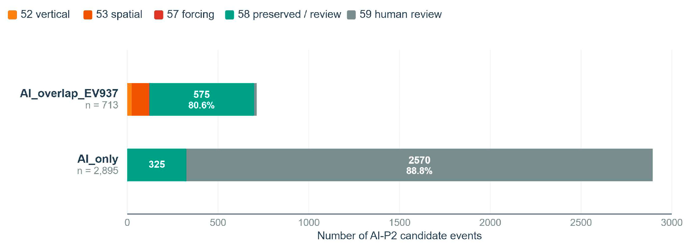
The 3608 candidate events were labelled at the event level as follows: qcode 58 (preserved/review event candidate) 900, qcode 59 (human review) 2586, qcode 53 (spatial deviation) 93, qcode 52 (vertical/layer inconsistency) 24 and qcode 57 (external-forcing mismatch or absence) 5. The distribution differs sharply by catalogue relation (

Table 4. Event-level AI-P3 qcode distribution.

Catalogue Relation	n (Events)	qcode 52	qcode 53	qcode 57	qcode 58	qcode 59
AI_overlap_EV937	713	24	93	5	575	16
AI_only	2895	0	0	0	325	2570
Total	3608	24	93	5	900	2586

) and is illustrated in Figure 4. Among the 713 EV937-overlapping candidates, most were interpretable or preserved (575 as qcode 58), with a smaller number assigned to inconsistency or mismatch labels (93 spatial, 24 vertical, 5 forcing) and only 16 left to review. Among the 2895 AI-only candidates, 325 received qcode 58 through adjacent-station co-occurrence support and 2570 were left as qcode 59, human-review cases; none were assigned a sensor-error qcode automatically. Overall, 2595 candidates were flagged as high review, 438 as mid and 575 as low. The contrast between the two catalogue relations is the key pattern: EV937-supported candidates are largely preserved (575 of 713 as qcode 58), whereas AI-only candidates lacking independent support are overwhelmingly routed to human review (2570 of 2895 as qcode 59) rather than being classified as false positives—a direct expression of the framework’s conservative, non-destructive design.

3.5. Final Additive Integration and Event Preservation

Integration attached the AI fields to 1,000,007 AI-applicable surface points with verified value invariance (water_temp, qc_temp2 and qcode_temp2 identical before and after). A total of 11,244 points received an AI event flag (qcode 58: 3276; 59: 7425; 53: 447; 52: 85; 57: 11). The preservation mask comprised 3276 points and the restore mask 53 points, of which 51 had been flagged as suspect and 2 as fail by Phase-2 QC. These 53 restore-candidate points correspond to 27 distinct events (grouped by event identifier). Metadata for these restore-candidate events are provided in Table S6. The preserve rate is thus about 0.33% of AI-applicable surface observations and the restore rate about 0.005%. All 53 restore-candidate points had previously carried Phase-2 gradient (qcode 21) or spike (qcode 23) flags and were treated as physically plausible regional-event candidates—for example, warm-season upwelling- or typhoon-consistent cooling episodes—rather than automatic failures. The framework is therefore conservative and does not over-restore data (station-wise preserve/restore counts are given in Table S4); original temperature values and Phase-2 flags remained unchanged.

3.6. Effects on Bulk Statistics and Event-Scale Cooling

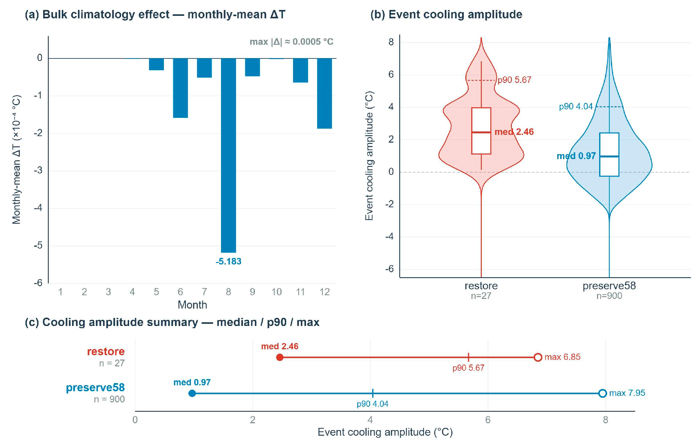
At the climatological scale, the effect of preservation and restoration was negligible. The maximum monthly mean temperature change was about 0.0005 °C for both the restore-only and the preserve-event comparisons (largest in August), and long-term as well as summer minima were unchanged at every station. Bulk monthly climatology was therefore not distorted. The contrast between the negligible monthly mean change and the substantial event-scale cooling is summarised in Figure 5.

At the event scale, by contrast, the preserved signals were substantial (

Table 5. Final integration outcomes and event-scale cooling amplitudes.

Quantity	Value	Notes
AI-applicable surface points	1,000,007	5 surface stations; values invariant
AI event-flagged points	11,244	qcode 58 = 3276
		qcode 59 = 7425
		qcode 53 = 447
		qcode 52 = 85
		qcode 57 = 11
Preserve mask (qcode 58)	3276 points (≈0.33%)	preserved/review event candidates
Restore mask	53 points (≈0.005%)	51 from suspect,
		2 from fail,
		27 distinct events
Max monthly mean Δ	≈0.0005 °C	restore-only and preserve-event;
		station-wise minima unchanged
Restore cooling amplitude	median 2.46 °C;	n = 27; 66.7% cooling-dominant
	p90 5.67;
	max 6.85 °C
Preserve58 cooling amplitude	median 0.97 °C;	n = 900; 59.6% cooling-dominant
	p90 4.04;
	max 7.95 °C

). The 53 restore-candidate points were grouped into 27 distinct restore events for event-scale amplitude analysis. Defining event cooling amplitude as the pre-event 6–12 h mean temperature minus the event minimum, the restore events (n = 27) had a median cooling amplitude of 2.46 °C, a 90th percentile of 5.67 °C and a maximum of 6.85 °C, with 66.7% cooling-dominant; the preserved qcode-58 events (n = 900) had a median of 0.97 °C, a 90th percentile of 4.04 °C and a maximum of 7.95 °C, with 59.6% cooling-dominant. Event-scale cooling amplitudes by AI event label are given in Table S5. The contrast between the two scales is the central quantitative result: the same operation that leaves monthly mean temperature essentially unchanged (≤0.0005 °C) preserves event-scale cooling of up to roughly 8 °C. The negligible climatological effect and the substantial event-scale preservation are of entirely different magnitudes, so the framework protects short-lived, physically plausible regional cooling candidates without perturbing the bulk temperature distribution, and additionally surfaces context-departing candidates missed by standard QC (the AI-only qcode-58 and human-review cases) for expert examination. 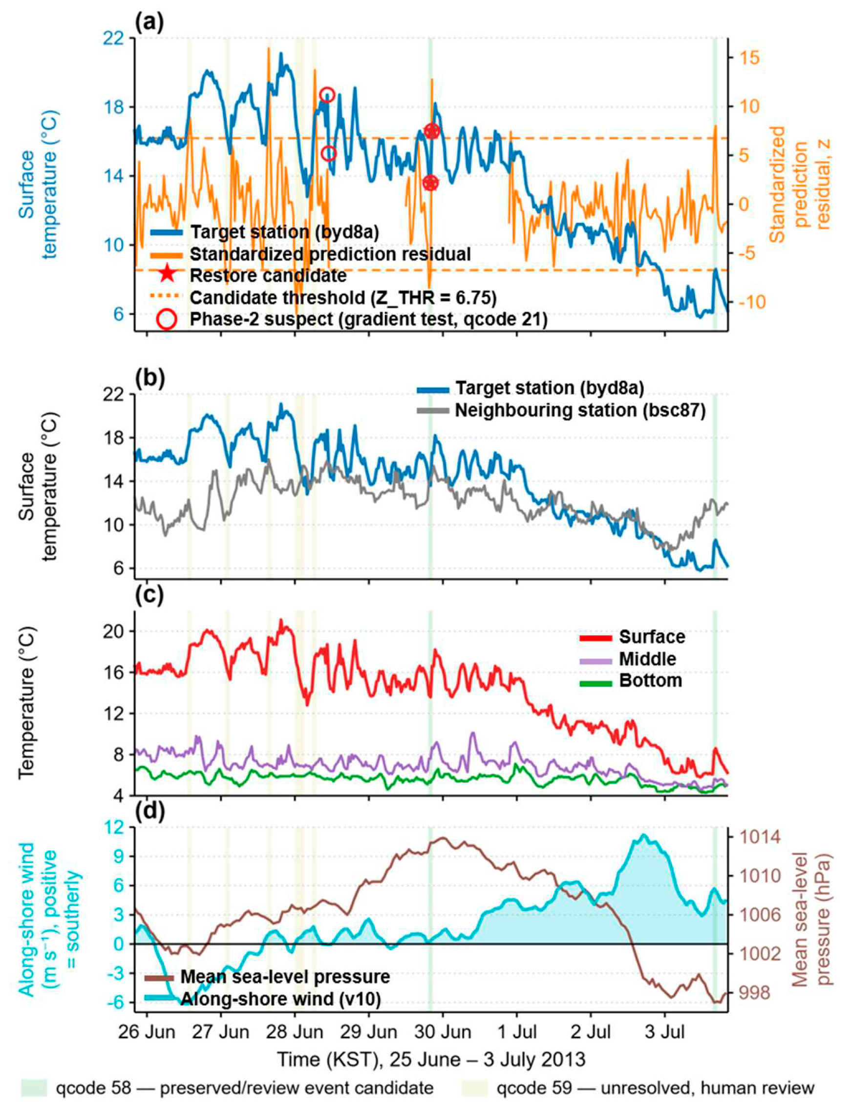Representative preserved/restored events are shown in Figure 6 and Figure 7.

Figure 5. Bulk-temperature effects and preserved event-scale cooling. (a) Monthly mean temperature changes after additive integration. (b,c) Cooling-amplitude distributions and summary statistics for restore events and preserved qcode-58 events.

Figure 5. Bulk-temperature effects and preserved event-scale cooling. (a) Monthly mean temperature changes after additive integration. (b,c) Cooling-amplitude distributions and summary statistics for restore events and preserved qcode-58 events.

Figure 6. Event-preservation framework applied to an upwelling-consistent cooling event at byd8a, 25 June–3 July 2013. (a) Surface temperature with the standardised prediction residual, the candidate threshold, restore candidates and Phase-2 suspect points. (b) Surface temperature at the target station and at the neighbouring station, showing spatial coherence. (c) Temperature at the surface, middle and bottom layers, showing the vertical structure. (d) Along-shore wind and mean sea-level pressure from ERA5. Shading marks the event-level qcode assigned by AI-P3. Panels (b–d) show the three physically interpretable axes used for classification: spatial coherence, vertical consistency and atmospheric forcing. Times are KST.

Figure 6. Event-preservation framework applied to an upwelling-consistent cooling event at byd8a, 25 June–3 July 2013. (a) Surface temperature with the standardised prediction residual, the candidate threshold, restore candidates and Phase-2 suspect points. (b) Surface temperature at the target station and at the neighbouring station, showing spatial coherence. (c) Temperature at the surface, middle and bottom layers, showing the vertical structure. (d) Along-shore wind and mean sea-level pressure from ERA5. Shading marks the event-level qcode assigned by AI-P3. Panels (b–d) show the three physically interpretable axes used for classification: spatial coherence, vertical consistency and atmospheric forcing. Times are KST.

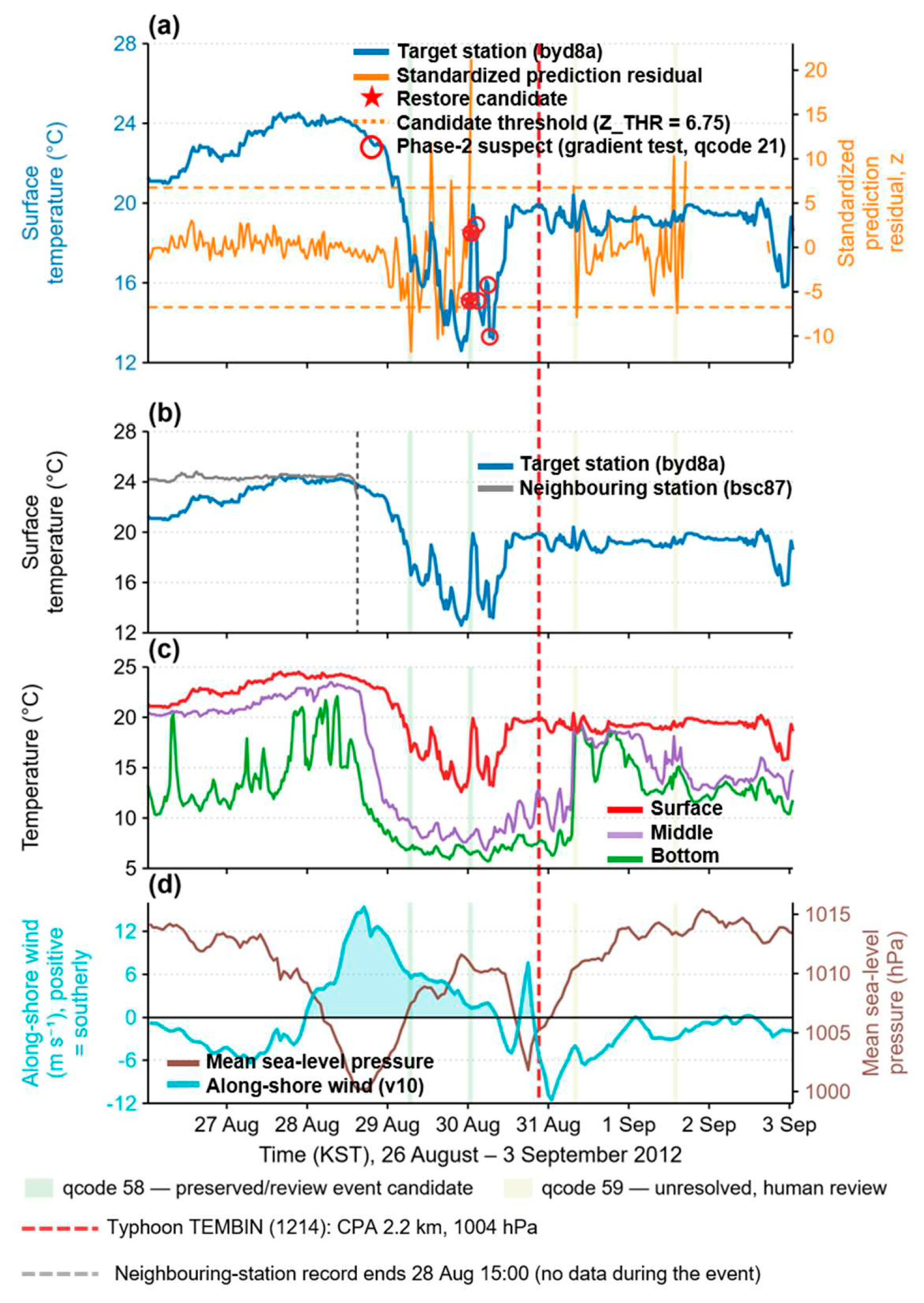
Figure 7. Event-preservation framework applied to a typhoon-related cooling event at byd8a, 26 August–3 September 2012. (a) Surface temperature with the standardised prediction residual, the candidate threshold, restore candidates and Phase-2 suspect points. (b) Surface temperature at the target station and at the neighbouring station, showing spatial coherence. (c) Temperature at the surface, middle and bottom layers, showing the vertical structure. (d) Along-shore wind and mean sea-level pressure from ERA5. Shading marks the event-level qcode assigned by AI-P3. The vertical dashed line marks the closest point of approach of Typhoon TEMBIN (1214), at 2.2 km with a central pressure of 1004 hPa. The neighbouring-station record ends on 28 August, so no spatial comparison is available during the event itself. Times are KST.

Figure 7. Event-preservation framework applied to a typhoon-related cooling event at byd8a, 26 August–3 September 2012. (a) Surface temperature with the standardised prediction residual, the candidate threshold, restore candidates and Phase-2 suspect points. (b) Surface temperature at the target station and at the neighbouring station, showing spatial coherence. (c) Temperature at the surface, middle and bottom layers, showing the vertical structure. (d) Along-shore wind and mean sea-level pressure from ERA5. Shading marks the event-level qcode assigned by AI-P3. The vertical dashed line marks the closest point of approach of Typhoon TEMBIN (1214), at 2.2 km with a central pressure of 1004 hPa. The neighbouring-station record ends on 28 August, so no spatial comparison is available during the event itself. Times are KST.

4. Discussion

4.1. Residual Magnitude Alone Is Insufficient

Machine-learning QC methods that learn the behaviour of normal data and flag departures from it have advanced the automatic detection of anomalous observations [16,17,18], including integrated imputation-and-detection approaches based on transformer and BiLSTM architectures [22,23,24] and semi-supervised frameworks designed to accommodate diverse marine environments [25,26,27]. A recurring difficulty, however, is that univariate or threshold-based detection performs poorly when anomalies are embedded within a strong seasonal component, where quartile- or Z-score-based rules fail to isolate genuine outliers [19,20,21]. Consistent with this, the prediction residuals of AI-P1 successfully identified statistically unexpected observations, but residual magnitude and sign alone did not determine whether a departure reflected a sensor-related artefact or a physically plausible coastal event: single-axis, residual-only separability between sensor-like anomalies and regional-event candidates was close to random (direction-free AUC 0.52–0.56; the residual is not used to define either group, so this figure is not affected by the circularity that applies to the physical axes). Crucially, the standardised residuals of regional-event candidates were not smaller than those of the sensor-like reference group but were comparable or larger (median standardised residual: sensor 7.70, upwelling-candidate 10.07, typhoon-related 8.72), so a larger residual cannot be read as stronger evidence of malfunction. These results indicate that AI prediction residuals are best treated as evidence of statistical unexpectedness—a broad anomaly-candidate signal—rather than as proof of sensor error.

4.2. Multiaxis Consistency Improves Interpretability

The distinction between a sensor-like anomaly and a physically plausible regional event emerged not from residual magnitude but from the joint behaviour of spatial coherence across neighbouring stations, vertical consistency between the surface and bottom layers, and physical forcing from wind and typhoon passage. Combining these physically interpretable axes yielded high separability between the reference and candidate groups within the axis space used to define them, with a cross-validated mean AUC of 0.987 and a pooled out-of-fold AUC of 0.981 (internal operational separability, not external validation), far exceeding residual-only discrimination. The reason these axes are informative is physical rather than merely statistical: a sensor fault at a single station is unlikely to reproduce a response in which neighbouring stations cool simultaneously, the bottom layer cools coherently with the surface, and the cooling coincides with along-shore, upwelling-favourable wind. Such multi-station, multi-layer, forcing-consistent co-occurrence is difficult to reconcile with a localised instrument artefact, and it is observable only because the array provides simultaneous neighbouring and vertical measurements. This separability should nonetheless be interpreted as internal operational separability among physically defined reference/candidate groups within the chosen discriminant space, not as independent confirmation of true event identity: because the sensor-like and upwelling-candidate groups were defined partly using the same physical axes, the multivariate result quantifies separability within the framework rather than validating event identity against an external ground truth. Consistent with this interpretation, the pairwise analysis further showed that spatial coherence and southerly-wind forcing dominate the separation of sensor-like anomalies from regional-event candidates, whereas vertical coherence (AUC 0.790) is the axis that best distinguishes upwelling-candidate from typhoon-related events.

4.3. Event-Preserving QC and Overscreening Risk

Reference-based QC that compares observations against external SST products can be vulnerable to overscreening in dynamically variable regions, where reference fields fail to resolve fine-scale or rapidly evolving thermal structure and valid observations are consequently flagged [51,52,53,54]. Recent machine-learning signal-processing work has also emphasised the need to avoid distorting inherent signal characteristics during anomaly correction or reconstruction [28,29,30]. The present framework responds to these concerns not by replacing conventional QC but by adding a physically interpretable preservation layer. Two design choices follow from this stance. First, to avoid circularity with the buoy temperature target, SST reference products are not used as inputs or calibration labels; spatial coherence, vertical consistency, and atmospheric forcing serve as the discriminant axes instead. The satellite comparison reported in Section 4.6 was carried out after the analysis was complete and is presented as a sanity check rather than as validation. Second, the framework is additive and non-destructive: Phase-3 results are written to separate fields, and the original temperature, qc_temp2, and qcode_temp2 values are never modified. Together, these choices reframe the goal of QC in dynamic coastal regions from automatic removal toward evidence-based review and preservation of physically plausible events.

4.4. Physical Plausibility of Abrupt Cooling

Abrupt cooling in coastal temperature records may be a sensor artefact, but it can also arise from real oceanographic processes. The western margin of the East Sea is a dynamically variable region shaped by interactions between the East Korea Warm Current and cold coastal waters [33,34,35], a setting in which strong short-term thermal variability can occur. In the southwestern East Sea, southerly and southwesterly winds drive coastal upwelling modulated by along-shore currents, stratification, and topography [36,37,38]; along the southern coast of Korea, upwelling has persisted for more than a month after upwelling-favourable winds weakened, producing a strong coastal–offshore temperature contrast [39,40,41]. Typhoon passages can generate rapid surface cooling of up to about 8 °C through entrainment, vertical mixing, and Ekman upwelling [42,43,44,45,46,47], and single-point surface observations are insufficient to resolve the vertical structure of these responses [48,49,50]. These studies do not directly validate the individual buoy events examined here because their case regions and observational settings differ from the present stations; rather, they demonstrate that rapid and persistent cooling is physically plausible in the broader Korean coastal and East Sea margin system. Accordingly, the regional-event labels used here should be interpreted as physically supported candidates rather than confirmed upwelling events.

4.5. Operational Implications

High-frequency coastal buoys underpin operational systems for coastal prediction and marine-disaster response [1,2,3,4,5,6], including high-water-temperature advisory systems linked to threshold-based criteria and substantial aquaculture losses [7,8,9,10,59]. In such settings, episodic but real coastal events can be mistaken for errors, and the cost of erroneously removing them is not merely statistical. The present framework functions as a decision-support layer rather than an automatic deletion tool. Its outputs distinguish graded review and preservation states: a prediction-residual candidate is recorded with qcode 51, which denotes an anomaly candidate only and does not by itself indicate a sensor error; qcode 58 marks a possible regional event to be preserved and reviewed; and qcode 59 marks unresolved cases requiring human review. A restore mask further identifies records that Phase-2 QC flagged as suspect or fail but that carry physically plausible event support and may therefore warrant reinstatement for a given analysis. A further asymmetry supports this design: preserving or restoring these events changes long-term monthly mean temperatures negligibly (≤0.0005 °C) while retaining substantial event-scale cooling amplitude (restore events: median 2.46 °C, maximum 6.85 °C; preserved qcode-58 events: median 0.97 °C, maximum 7.95 °C), so event preservation protects short, strong signals without perturbing the climatological record. Because the integration is value-invariant—the original water_temp, qc_temp2, and qcode_temp2 are identical before and after—a downstream user can choose whether to include or exclude flagged events without any loss of the original record. In operational QC, providing review priorities and preservation flags is therefore a safer default than automatic removal.

The balance between the two error types depends on what the record is for, and the framework leaves that balance adjustable rather than fixing it. Two errors are possible: a genuine instrument fault may be preserved as an event, contaminating the record, or a genuine event may be left flagged, discarding a real signal. Their costs are not symmetric here. Preserving the qcode-58 events shifts derived monthly means by at most 0.0005 °C, so a climatological analysis is largely indifferent to the choice, whereas removing them discards cooling of up to about 8 °C at event scale—the signal an aquaculture warning system exists to detect. Where recall matters more than review effort, the candidate threshold can be relaxed: lowering Z_THR from 6.75 to 5.00 raises the recall of upwelling reference events from 0.65 to 0.83, at the cost of 1.9 times as many anomaly candidates to inspect (Table S3), against about 91 anomaly candidates per station-year of effective record at the adopted threshold. Applications that need a stable long-term record can keep the adopted threshold or exclude qcode-58 events altogether. Because the integration leaves the original values and the Phase-2 flags unchanged, this choice is made downstream, and two users of the same dataset can make it differently.

4.6. Limitations

The sensor-like reference group is not independently confirmed. The buoys are serviced on a monthly schedule, when sensor operation is checked and the sensors are cleaned, but records that would link an individual servicing action to a specific station and time were not available to us. No member of this group is therefore verified as an instrument fault. The criteria used to define it describe the absence of spatial, vertical and forcing support, rather than positive evidence of an instrument fault. The group should accordingly be interpreted as a sensor-like reference group, not as a set of confirmed sensor failures.

The separability measures reported here are not independent of the group definitions. The same axes are used both to define the reference and candidate groups and to discriminate between them, so the separability reported in Section 3.2 and Table 2 is partly tautological by construction. The pairwise value of 1.000 for the sensor-like versus upwelling-candidate contrast should be read in this light, as should the multivariate cross-validated mean AUC of 0.987. The one contrast in this study that is anchored outside the buoy signal is the sensor-like versus typhoon-related comparison, in which the typhoon group is defined from best-track data; the corresponding AUC values of 0.848 and 0.851 are substantially lower than 1.000, and the lower values in this contrast illustrate that the shared-definition contrasts should not be interpreted as independent classification performance. The two comparisons also differ in the physical processes involved, so the difference between them is not a quantitative estimate of the inflation. An audit against maintenance records remains the most direct route to an independently defined sensor-like reference group.

Independent verification of individual events is intrinsically constrained. We compared eight large events, spanning six different years, against a satellite-only level-3 sea surface temperature product as a post hoc sanity check (Figure S6). Satellite SST provides only limited constraint on nearshore conditions, for reasons inherent to the sensors themselves: infrared retrievals fail in the presence of cloud, while microwave retrievals have a resolution of about 25 km and are not made close to land [60]. Between 47% and 51% of each 0.5° × 0.5° box was excluded as land or as coastally contaminated, and the buoys sit 1.8–2.8 km from the shoreline, that is, within the band where satellite retrieval is weakest. Where clear-sky retrievals were available, the satellite fields resolved cooling of at most 2.6 °C against buoy-recorded amplitudes of 7.4–16.7 °C, a ratio with a median of 0.15. The discrepancy is not random: for the largest event in the set, a typhoon that cooled the buoy record by 16.7 °C, cloud cover left almost no clear-sky retrieval within the event window, so the event that would have been most useful for verification was the one the satellite could not see. The timing also differs, with the satellite minimum lagging the buoy minimum by a median of 22 h; most buoy minima occurred at night, which a daily composite cannot resolve. In most of the events examined here, the satellite coastal and offshore band averages remained close to one another, while the buoy record departed from both, indicating that the sharp nearshore excursions recorded by the buoy were not resolved in these band-averaged satellite series. This is consistent with an independent assessment of eleven blended level-4 products against shallow subtidal temperature loggers, which found that they underestimate the thermal fingerprint of coastal upwelling—with average warm biases exceeding 2 °C at strongly upwelling sites—and recommended against their use in upwelling-dominated settings; the same study reports that level-3 data perform better than level-4 but remain spatially and temporally inconsistent along coastlines, and concludes that long-term in situ temperature monitoring networks are needed [56].

These constraints illustrate why high-frequency coastal buoy observations are needed in nearshore environments. Nearshore records are collected precisely where satellite retrieval is weakest and where the cross-shore gradient is steepest, so the independent observing systems available for such verification are also those most affected by cloud cover, coastal masking, land contamination and resolution limits in the nearshore zone. We therefore describe these events throughout as physically plausible candidates rather than as confirmed regional events, and we treat the satellite comparison as a sanity check rather than as validation.

The atmospheric comparison does not validate the temperature response. The KMA Pohang buoy was used as a regional atmospheric alibi to check the reliability of the ERA5 forcing fields, not as a direct validation of the temperature responses recorded at individual NIFS stations.

The prediction-residual component covers only part of the record. The prediction-residual model was applied to the surface layer of five stations. The middle and bottom layers, and the most recently deployed station (fggo3), which has a record too short to train a station-specific model, are outside its scope; for those channels, the framework operates on the physical axes alone.

The threshold sensitivity result applies to the ranges examined. Varying the spatial coherence threshold from |z| < 1.5 to |z| < 2.5 and the vertical shape-correlation threshold from 0.25 to 0.45 changed the preserved-point count by at most 1.0% and left the restore-candidate count unchanged (Table S8). This does not exclude larger changes outside the ranges tested, and it partly reflects the ordering of the decision rules rather than an intrinsic robustness of either threshold considered alone.

4.7. Future Work

Three lines of work follow directly from these limitations. First, an audit against instrument maintenance and replacement records would allow the sensor-like reference group to be defined independently of the buoy signal and would make the separability measures interpretable as validation rather than as internal separability. Second, independent event evidence—satellite chlorophyll, a wind-stress curl index, or in situ current profiles—could promote a subset of the candidate events toward confirmed regional events; for the coastal zone, observing systems that resolve the cross-shore gradient would be more informative than band-averaged satellite fields. Third, extending the prediction-residual model across layers and stations, including the shorter records, would broaden the coverage of the anomaly-candidate stage. We also intend to connect the preserved event catalogue to downstream ecological analyses, for which the preservation of event-scale cooling is the practical motivation for this framework.

5. Conclusions

We developed a machine-learning-assisted, physics-guided, event-preserving quality-control framework for coastal buoy temperature observations in the western coastal waters of the East Sea (Japan Sea). AI prediction residuals were useful for broad anomaly-candidate detection but insufficient for separating sensor-like anomalies from regional-event candidates, with a residual-only separability of only 0.52–0.56; the standardised residuals of upwelling-candidate and typhoon-related events equalled or exceeded those of the sensor-like reference group, so residual magnitude cannot itself indicate malfunction. Physically interpretable axes—spatial coherence, vertical consistency and atmospheric/typhoon forcing—separated sensor-like anomalies from regional-event candidates, reaching pairwise AUC values of 1.000 for the strongest axes and a combined-axis cross-validation mean AUC of 0.987 (pooled out-of-fold 0.981); this separability reflects internal operational separability among physically defined groups rather than independent confirmation of event identity. The final integration preserved regional-event candidates conservatively without changing original observations or existing QC flags: bulk monthly climatology was nearly unchanged (at most about 0.0005 °C), whereas event-scale cooling signals were substantial (restore events median 2.46 °C; preserved events median 0.97 °C, with maxima approaching 8 °C). The framework provides a practical, transferable way to prevent the false removal of coastal upwelling- and typhoon-consistent temperature responses in coastal ocean-observing records, treating AI prediction residuals as evidence of statistical unexpectedness and reserving event classification for physically interpretable, multi-station criteria.