Refined Prediction of Strain-Softening Parameters of Marine Soft Clay Using Cyclic T-Bar Penetration Tests

Abstract

T-bar penetrometers are widely utilized for measurements of strength characteristics of soft clay in offshore field investigations and laboratory tests. To obtain strain-softening parameters of marine soft clay, it is necessary to conduct cyclic T-bar tests below the critical penetration depth. Therefore, this study conducted CEL large-deformation finite-element analyses to simulate the entire penetration process of T-bar in strain-softening soils. An equation for predicting the critical penetration depth is proposed, taking into account both the amount and the rate of strength reduction of clay. The numerical results indicate that the minimum depth for initiating the pull-out phase of the cyclic test is the full-flow penetration depth plus three times the T-bar diameter, which ensures that the surrounding soil remains in a full-flow mechanism throughout the cyclic test. Moreover, a refined resistance degradation model is proposed, which corrects a defect in the existing model, which is that when the number of cycles is equal to N₉₅, the predicted result of the model does not reach 95% degradation in penetration resistance. Then, an estimation method for strain-softening parameters of soft clay is developed. The method based on the refined resistance degradation model is verified by comparing the estimated values with the numerical simulation results in this paper and the available test data.

1. Introduction

Strain softening is a common behavior of marine soft clay. The strain-softening behavior of soft clay has significant influences on such marine structures as pipelines, anchoring systems, and offshore foundations. In recent years, full-flow penetrometers of T-bar have been widely utilized in offshore field investigations and laboratory tests. An important advantage of T-bar is its potential to obtain strain-softening parameters of marine clay in situ, by means of cyclic penetration and extraction tests. Such tests are generally conducted after the penetrometer has been advanced to a given depth, with the probe being cycled several times within a narrow depth range of three diameters of the probe, in order to remold the soil locally within a rectangular slot. Further investigations of cyclic T-bar penetration behavior have shown that cyclic remolding may not occur in stiffer soils or under lower overburden stress conditions [1,2]. Experimental evidence has demonstrated that an open cavity may develop under such conditions, potentially leading to errors in the estimation of strain-softening parameters [3,4,5,6]. The shallow flow mechanism has been shown to significantly affect cyclic T-bar test results, as water entrainment in the cavity can cause continuous strength loss and lead to remolded strength values much lower than those estimated from deep cycles without a trapped cavity [5]. Therefore, the T-bar should be penetrated to a sufficient depth prior to the pull-out phase to ensure a full-flow mechanism during cyclic T-bar tests. While some studies have adopted a fixed depth of 10D as being adequate for pull-out initiation [7], recent numerical simulations suggest that the minimum pull-out initiation depth should exceed the full-flow penetration depth d_ff [8]. However, the quantitative excess beyond d_ff has not yet been explicitly specified. Accordingly, one of the objectives of this study is to determine the minimum depth required for initiating the pull-out phase of the cyclic test.

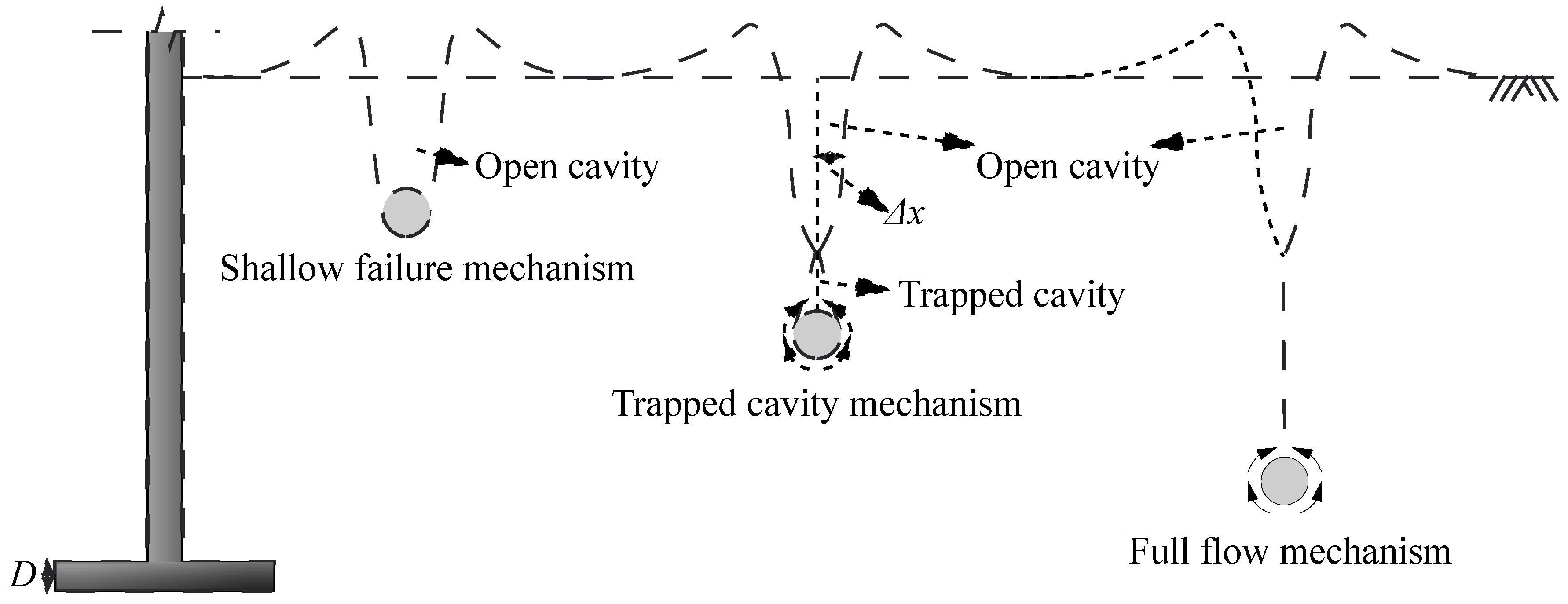
As shown in Figure 1, the failure mechanism of the penetrometer from shallow to deep penetration depths can be divided into three stages: the shallow failure mechanism with an open cavity above the penetrometer, the trapped-cavity failure mechanism with a trapped cavity at the crown of the penetrometer, and the full-flow failure mechanism, in other words, the deep failure mechanism under which the trapped cavity is completely closed [9,10,11,12,13]. In Figure 1, the gap between the cavity wall and the line of symmetry is marked as Δx.

Therefore, during the entire penetration process of T-bar, there are two critical penetration depths: the trapped-cavity penetration depth (d_tc), where the trapped cavity is formed, and the full-flow penetration depth (d_ff), also termed the deep penetration depth, where the trapped cavity has completely vanished. The trapped-cavity failure mechanism was not considered in previous interpretations of shallow T-bar penetration behavior [12]. Therefore, the deep penetration depth reported in the previous study can be interpreted as the trapped-cavity penetration depth d_tc [12]. A trapped cavity may form behind the T-bar, resulting in a bearing factor approximately 12% lower than that associated with the full-flow mechanism [9]. Thus, they proposed that the full-flow penetration depth d_ff should be the critical depth where the trapped cavity is completely closed. A systematic procedure has also been developed to account for the trapped-cavity effect, thereby improving the interpretation of soil strength from T-bar penetration resistance data [11]. It should be noticed that the above-mentioned studies did not take into account the soil-softening behaviors. Large-deformation finite-element analyses have recently been used to investigate strain-softening behavior during initial penetration, and an empirical formula has been established for the trapped-cavity penetration depth of the T-bar [1]. An equation for the full-flow penetration depth of the T-bar has been proposed, but the ductility-softening parameter, which reflects the rate of clay strength reduction, was not considered [8].

Moreover, once the full-flow penetration depth is determined, the strain-softening parameters of soft clay can be interpreted from the resistance degradation with cyclic full-flow penetration tests. The gradual degradation in resistance during cyclic tests needs to be modeled by decay functions as an aid for interpreting the strain-softening parameters. The degradation in penetration resistance during cyclic testing can be represented using the following expression [14]:

$${\displaystyle \frac{q_n}{q_{\mathrm{in}}}}={\displaystyle \frac{q_{\mathrm{rem}}}{q_{\mathrm{in}}}}+\left(1-{\displaystyle \frac{q_{\mathrm{rem}}}{q_{\mathrm{in}}}}\right){\mathrm{e}}^{-3\left(n-0.5\right)/N_{95}}$$

(1)

where q_n is penetration resistance at the nth penetration cycle (n = 0.5 for the first penetration, n = 1 for the first extraction, and so on), q_in and q_rem are the first penetration and the remolded penetration resistance, respectively, and N₉₅ is the number of cycles required for 95% degradation in resistance, i.e., 0.95 (q_in − q_rem).

Comparison with in situ cyclic test results indicates that Equation (1) cannot accurately reproduce the actual degradation of penetration resistance because its initial slope is too moderate; therefore, the exponential degradation can be anchored to the first extraction rather than the first insertion [15]:

$${\displaystyle \frac{q_n}{q_{\mathrm{in}}}}={\displaystyle \frac{q_{\mathrm{rem}}}{q_{\mathrm{in}}}}+\left({\displaystyle \frac{q_{\mathrm{ext}}}{q_{\mathrm{in}}}}-{\displaystyle \frac{q_{\mathrm{rem}}}{q_{\mathrm{in}}}}\right){\mathrm{e}}^{-3\left(n-1\right)/N_{95}}$$

(2)

where q_ext is the first extraction resistance. Although this compromise improves the agreement with field test results to a certain extent, it is achieved at the expense of disregarding the initial penetration resistance, which is a crucial piece of information in the outcomes of the cyclic penetration test.

Based on the relative plastic strain accumulated during penetration and subsequent extraction, which accounts for 25% and 75% of the total shear strain over a full cycle, respectively, the first penetration and first extraction can be labeled as 0.25 and 0.75 [16], given by

$${\displaystyle \frac{q_n}{q_{\mathrm{in}}}}={\displaystyle \frac{q_{\mathrm{rem}}}{q_{\mathrm{in}}}}+\left(1-{\displaystyle \frac{q_{\mathrm{rem}}}{q_{\mathrm{in}}}}\right){\mathrm{e}}^{-3\left(n-0.25\right)/N_{95}}$$

(3)

This cycle-numbering convention has been widely adopted in subsequent studies [8,17,18].

By introducing a parameter β to Equation (3), a resistance degradation model was developed to balance the initial brittleness and the fully remolded state of the soil [19]. The model is given by

$${\displaystyle \frac{q_n}{q_{\mathrm{in}}}}={\displaystyle \frac{q_{\mathrm{rem}}}{q_{\mathrm{in}}}}+\left(1-{\displaystyle \frac{q_{\mathrm{rem}}}{q_{\mathrm{in}}}}\right){\mathrm{e}}^{-3{\left(\left(n-0.25\right)/N_{95}\right)}^{\beta }}$$

(4)

However, there is a defect in these models mentioned above, which is that when the number of cycles is equal to N₉₅, the predicted result of the model does not reach 95% degradation in penetration resistance.

According to the definition of N₉₅, the resistance at N₉₅ can be expressed by

$$q_{N_{95}}=q_{\mathrm{in}}-0.95\left(q_{\mathrm{in}}-q_{\mathrm{rem}}\right)=q_{\mathrm{rem}}+0.05\left(q_{\mathrm{in}}-q_{\mathrm{rem}}\right)$$

(5)

If both sides of this equation are divided by q_in, then the following formula can be obtained:

$${\displaystyle \frac{q_{N_{95}}}{q_{\mathrm{in}}}}={\displaystyle \frac{q_{\mathrm{rem}}}{q_{\mathrm{in}}}}+\left(1-{\displaystyle \frac{q_{\mathrm{rem}}}{q_{\mathrm{in}}}}\right)\times 0.05$$

(6)

Let n = N₉₅; then, the resistance $q_{N_{95}}$ can be calculated from Equation (4) as follows:

$${\displaystyle \frac{q_{N_{95}}}{q_{\mathrm{in}}}}={\displaystyle \frac{q_{\mathrm{rem}}}{q_{\mathrm{in}}}}+\left(1-{\displaystyle \frac{q_{\mathrm{rem}}}{q_{\mathrm{in}}}}\right){\mathrm{e}}^{-3{\left(\left(N_{95}-0.25\right)/N_{95}\right)}^{\beta }}$$

(7)

If we define the function $f\left(n\right)={\mathrm{e}}^{-3{\left(\left(N_{95}-0.25\right)/N_{95}\right)}^{\beta }}$, then the function f(n) should always provide a value of 0.05 at n = N₉₅. Evidently, these models do not satisfy this condition, and thus the resistance degradation model needs to be refined.

This study aims to explore the soil deformation mechanism during T-bar initial penetration and subsequent cyclic events through large-deformation finite-element (CEL) analyses, and to develop an estimation method for strain-softening parameters of soft clay based on cyclic T-bar tests. The novelty of this study lies in addressing three knowledge gaps: (i) proposing a quantitative relationship for the critical penetration depth that explicitly accounts for the ductility-softening parameter; (ii) identifying the minimum pull-out initiation depth required to maintain a full-flow mechanism throughout the cyclic test; and (iii) developing a refined resistance degradation model that overcomes the theoretical deficiency in the existing model, i.e., its failure to achieve the expected 95% degradation at n = N₉₅.

2. Finite-Element Analyses of T-Bar Initial Penetration

During penetration, the elements of soil around the T-bar significantly change their relative positions, such that strains of large magnitude develop and therefore affect the soil properties. The large-soil-deformation problem of T-bar penetration in this study is solved using the coupled Eulerian–Lagrangian (CEL) approach in the commercial finite-element package ABAQUS.

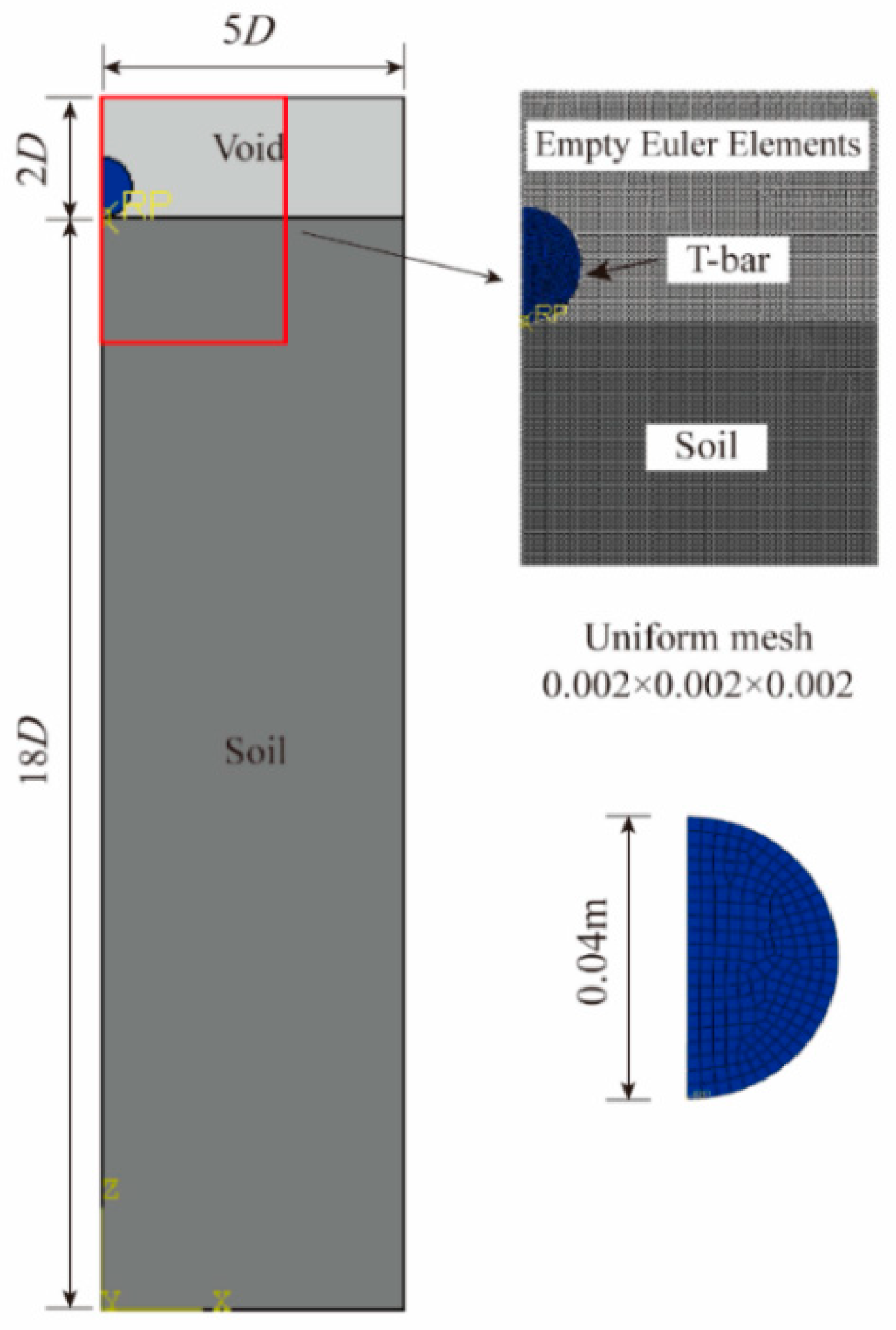
For all analyses in this study, only one half of the T-bar and soil domain was involved accounting for the symmetry, as shown in Figure 2. The T-bar is modeled as a Lagrangian rigid body. The soil was discretized using Eulerian elements of type EC3D8R. The Eulerian domain was chosen as 5D in horizontal and 20D in depth to avoid boundary effects (D is the diameter of the T-bar). The Eulerian mesh included the original soil domain and an overlying void layer with a thickness of 2D to allow the soil to flow into the empty Eulerian elements. The uniform mesh in the range of 16D in depth and 3D in horizontal was refined to D/20. It has been verified that further mesh refinement has little influence on the simulation results when the mesh size is smaller than D/20 [8]. In addition, a mesh sensitivity analysis was performed on a case with s_u/γ′D = 3, S_t = 5, and ξ₉₅ = 15 to ensure the reliability of the numerical results. Three mesh sizes, i.e., D/10, D/20, and D/25, were compared in terms of the computed penetration resistance. The results show that the difference between the D/20 and D/25 meshes is within 2%, whereas the D/10 mesh yields a deviation of about 8% from the D/20 mesh. Accordingly, the D/20 mesh was adopted in all subsequent analyses, as it provides sufficient accuracy with reasonable computational cost. The rest domains were set as gradually coarser mesh with the maximum element size near the boundary being about D/4. In the field tests, the length L and diameter D of the T-bar are 25 cm and 4 cm, respectively. Given that the end effect on the bearing factor becomes minimal when the aspect ratio L/D exceeds 6 [1], a plane-strain assumption was adopted in this study to reduce computational cost. Currently, only three-dimensional elements are available in CEL analyses. Therefore, in order to simulate the plane-strain condition, one element (with thickness D/20) was taken in the thickness direction of the model, and the two in-plane faces were constrained against moving in the thickness direction. The upper soil surface was free, and the remaining boundaries were fixed on the normal direction but free to move in the tangential direction.

As mentioned in most published papers, the penetration of T-bar in soft clay is under undrained conditions. Therefore, the clay was modeled as elastic: a perfectly plastic material obeying the Tresca yield criterion but extending to capture the strain-softening effect. The undrained shear strength at each integration point was updated at the beginning of each time increment using a widely adopted strain-softening model [14] as

$$s_{\mathrm{u}}=s_{\mathrm{u}0}\left[{\delta }_{\mathrm{rem}}+\left(1-{\delta }_{\mathrm{rem}}\right){\mathrm{e}}^{-3\xi /{\xi }_{95}}\right]$$

(8)

where s_u0 is the intact undrained shear strength, s_u is the current strength considering strain softening, δ_rem is the fully remolded strength ratio defined as the specific value of the fully remolded strength to the intact one (i.e., inverse of the soil sensitivity, S_t), which reflects the final amount of strength reduction, ξ is the accumulated absolute plastic shear strain, and ξ₉₅ represents the cumulative plastic shear strain corresponding to a 95% degradation in strength, which reflects the rate of strength softening and is also termed as the ductility parameter. The typical values of ξ₉₅ are within the range of 10–50. A consistent stiffness ratio of E/s_u = 300 (where E is the Young’s modulus) and Poisson’s ratio v = 0.495 were taken throughout the clay profile.

The general contact algorithm in ABAQUS was employed to simulate the interaction between the T-bar and soil. The interface was modeled as a frictional contact by specifying the Coulomb friction law together with limiting shear stress τ_max along the T-bar and soil interface. The Coulomb friction coefficient was set as a high value of μ = 1000 in order to allow the limiting shear stress τ_max to govern the soil failure. The limiting shear stress was defined using an adhesion factor α, which was taken to be equal to the remolded strength ratio δ_rem under the condition accounting for strain softening. The adhesion factor α is taken as δ_rem, implying that the limiting shear stress at the soil–probe interface corresponds to the remolded shear strength. This is justified by the fully rough nature of the probe surface and the severe remolding of the adjacent soil during cyclic penetration; under such conditions, the interface shear strength approaches the remolded strength of the clay. This assumption is consistent with the approach adopted in previous studies on T-bar penetration in soft clays [8,16].

A typical submerged unit weight of marine clay γ′ = 6 kN/m³ was adopted for all analyses. In the first step, the initial geostatic stress field was applied on the soil domain with coefficient of lateral earth pressure K₀ = 1, as the stable penetration resistance has been shown to be nearly unaffected by this coefficient [17]. In the next step, a downward velocity boundary condition was imposed at the reference point of the T-bar to insert itself into the soil at a specified depth, and the reaction force F_s during the penetration process can be acquired. It should be noted that the purpose of this paper is to evaluate the impact of strain softening on the T-bar test results; therefore, a velocity of 0.004 m/s (=0.1D), which is merely one-fifth of the penetration velocity recommended in the field test, was selected in the studies to disregard the influence of strain rate on the results. This setup is consistent with those adopted in previous finite-element analyses [8,20].

The T-bar bearing factor, N_t, can be calculated by Equation (9):

$$N_{\mathrm{t}}={\displaystyle \frac{F_{\mathrm{net}}}{A{s}_{\mathrm{u}0}}}={\displaystyle \frac{F_{\mathrm{s}}-F_{\mathrm{b}}}{A{s}_{\mathrm{u}0}}}$$

(9)

where F_net is the net penetration resistance, F_s is the total penetration resistance measured by the T-bar penetrometer, F_b is the buoyant force, and A is the cross-sectional area of T-bar. The buoyant force F_b can be obtained using an established formulation for T-bar penetration analysis [10].

3. Results of the Initial T-Bar Penetrations

3.1. Comparison with Existing Results

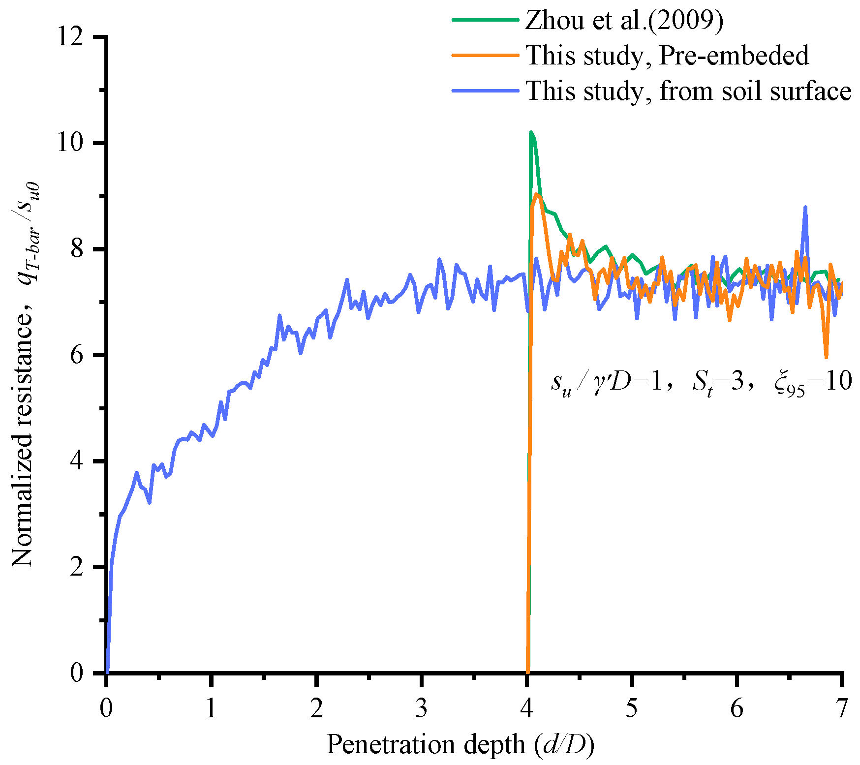
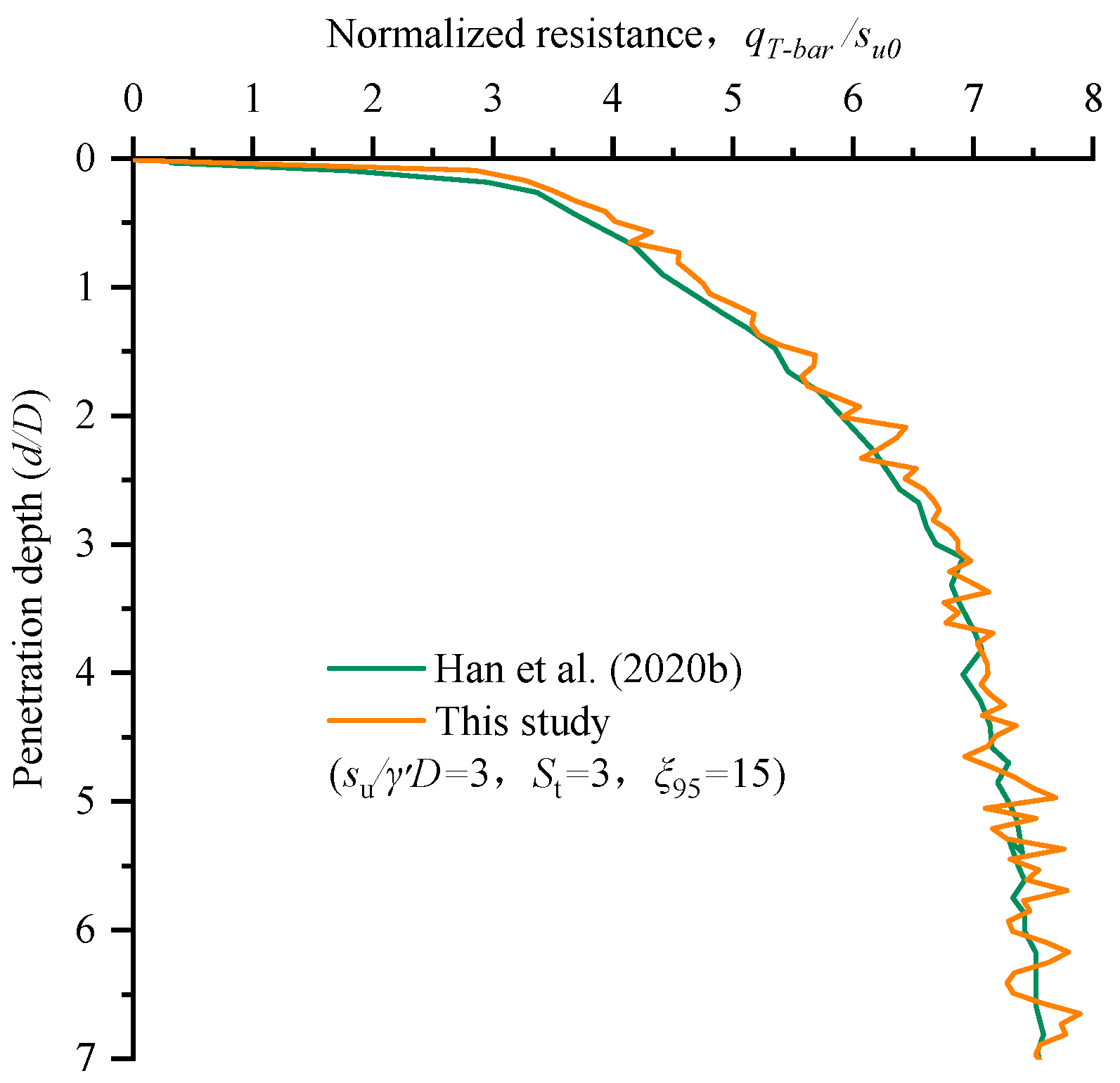
The RITSS method has been employed to simulate the penetration process of a pre-embedded T-bar [17]. In this paper, two different penetration approaches are utilized to reproduce the results. One penetrated from a depth of d/D = 4 (d is the depth from the soil surface), while the other started from the soil surface. Comparison of the results shows that the first approach produces results that nearly coincide with previous numerical results [17]. Although the initial penetration depths differ, the results obtained using the second approach tend to converge toward the previous numerical results after deep penetration [17]. The comparison between the present results and previous numerical results is shown in Figure 3.

An additional case involving penetration from the soil surface was also conducted for comparison with previous numerical results [8]. It can be seen from Figure 4 that the present result agrees well with previous numerical results [8]. The stable bearing factor N_t obtained from the present numerical simulation differs from that reported in [8] by approximately 3%.

3.2. Prediction of the Critical Depth

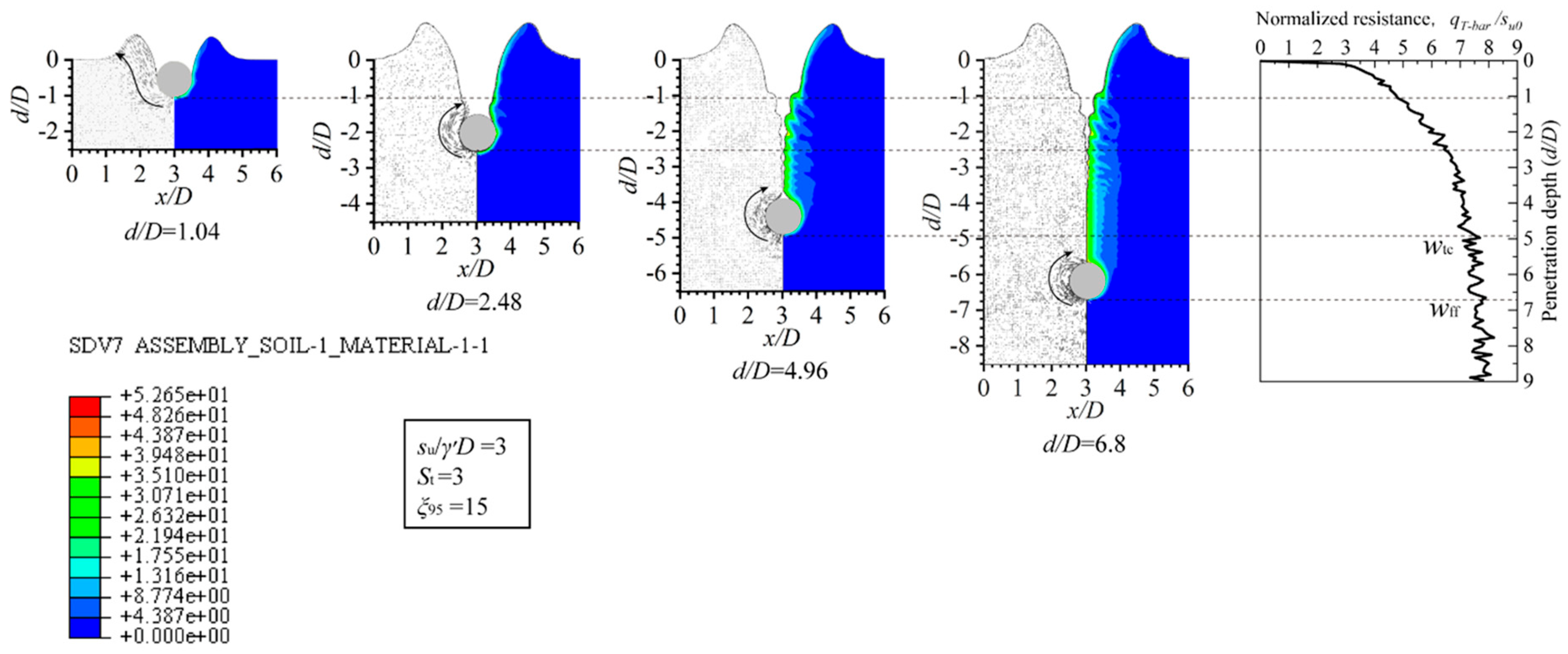
As mentioned in the introduction, in the entire penetration process of T-bar, there are two critical penetration depths: the trapped-cavity penetration depth (d_tc), where the trapped cavity is formed, and the full-flow penetration depth (d_ff), at which the trapped cavity is completely closed. For the case of s_u/γ′D = 3, S_t = 3, and ξ₉₅ = 15, the instantaneous velocity vectors and cumulative plastic strain contours of soil at various characteristic penetration depths are depicted in Figure 5. The cumulative plastic strain, which is stored in the solution-dependent state variable SDV7 in the user-defined subroutine (VUSDFLD), is used to quantify the degree of soil remolding during penetration. With the increase in penetration depth, the soil surface gradually heaves to accommodate the T-bar, and an open cavity is formed at the top of the T-bar. At d/D = 2.48, the height of the soil heave attains a maximum. Subsequently, with the continuous penetration, the soil at the crown of the T-bar gradually collapses and flows back. When d_tc/D reaches 4.96, the cavity wall touches the symmetry line of the model (i.e., Δx = 0, as marked in Figure 1), forming a trapped cavity. The trapped cavity remains with the T-bar penetrating deeper, but the volume of the trapped cavity gradually diminishes. At d_ff/D = 6.8, the trapped cavity vanishes completely, signifying that the full-flow mechanism is established. Subsequently, with further penetration, the bearing factor is kept unchanged.

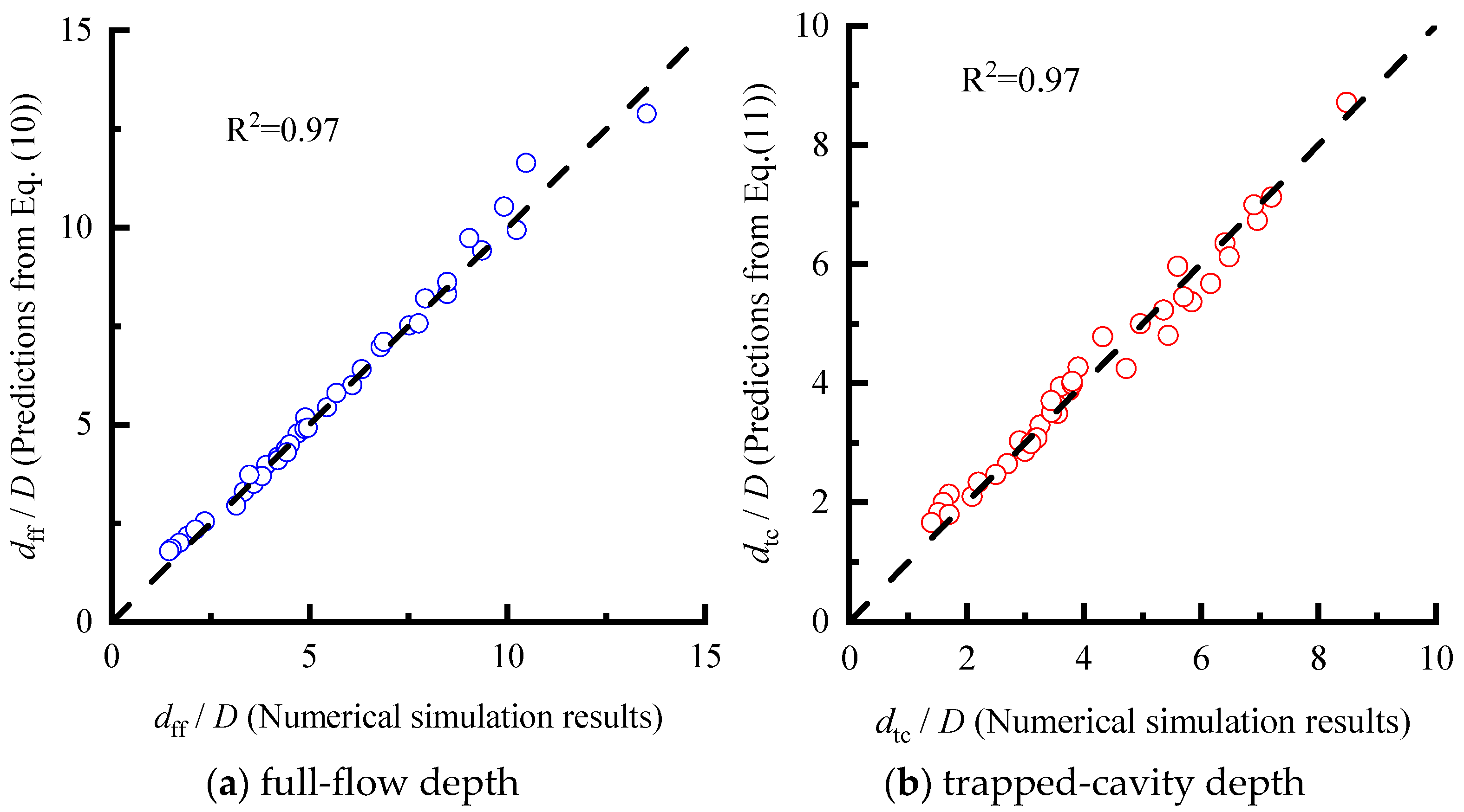
To investigate the influence of different soft soil parameters (s_u0, S_t, and ξ₉₅) on d_ff and d_tc, a total of 38 cases with varying combinations of these parameters were conducted, as presented in

Table 1. Model parameters.

su/γ′D	St	ξ95
0.3	3\5\10\20	15
1	2\3	10\15\20\30\40
1	5\10\20	15
3	2	10\20\30\40
3	3\5	10\15\20\30\40
3	10\20	15
4.8	2\3\5\10\20	15

. The values of d_ff and d_tc in each case are shown in Figure 6. Through performing regression analyses, best fits can be obtained by Equation (10) for d_ff and Equation (11) for d_tc.

$${\displaystyle \frac{d_{\mathrm{ff}}}{D}}=1.53+\left(0.04{\xi }_{95}+{\displaystyle \frac{4.1}{S_{\mathrm{t}}}}\right){\left({\displaystyle \frac{s_{\mathrm{u}}}{{\gamma }^{\prime }D}}\right)}^{\left(0.96-0.03{S_{\mathrm{t}}}^{0.13}\right)}$$

(10)

$${\displaystyle \frac{d_{\mathrm{tc}}}{D}}=1.26+0.99\times {\left(0.04{\xi }_{95}+{\displaystyle \frac{2.95}{S_{\mathrm{t}}}}{\displaystyle \frac{s_{\mathrm{u}}}{{\gamma }^{\prime }D}}\right)}^{\left(0.87+0.06S_{\mathrm{t}}\right)}$$

(11)

As shown in Figure 6, Equations (10) and (11) show good applicability with the simulated results (R² = 0.97). They can be used to predict the critical penetration depths, taking into account both the amount and the rate of strength reduction of clay.

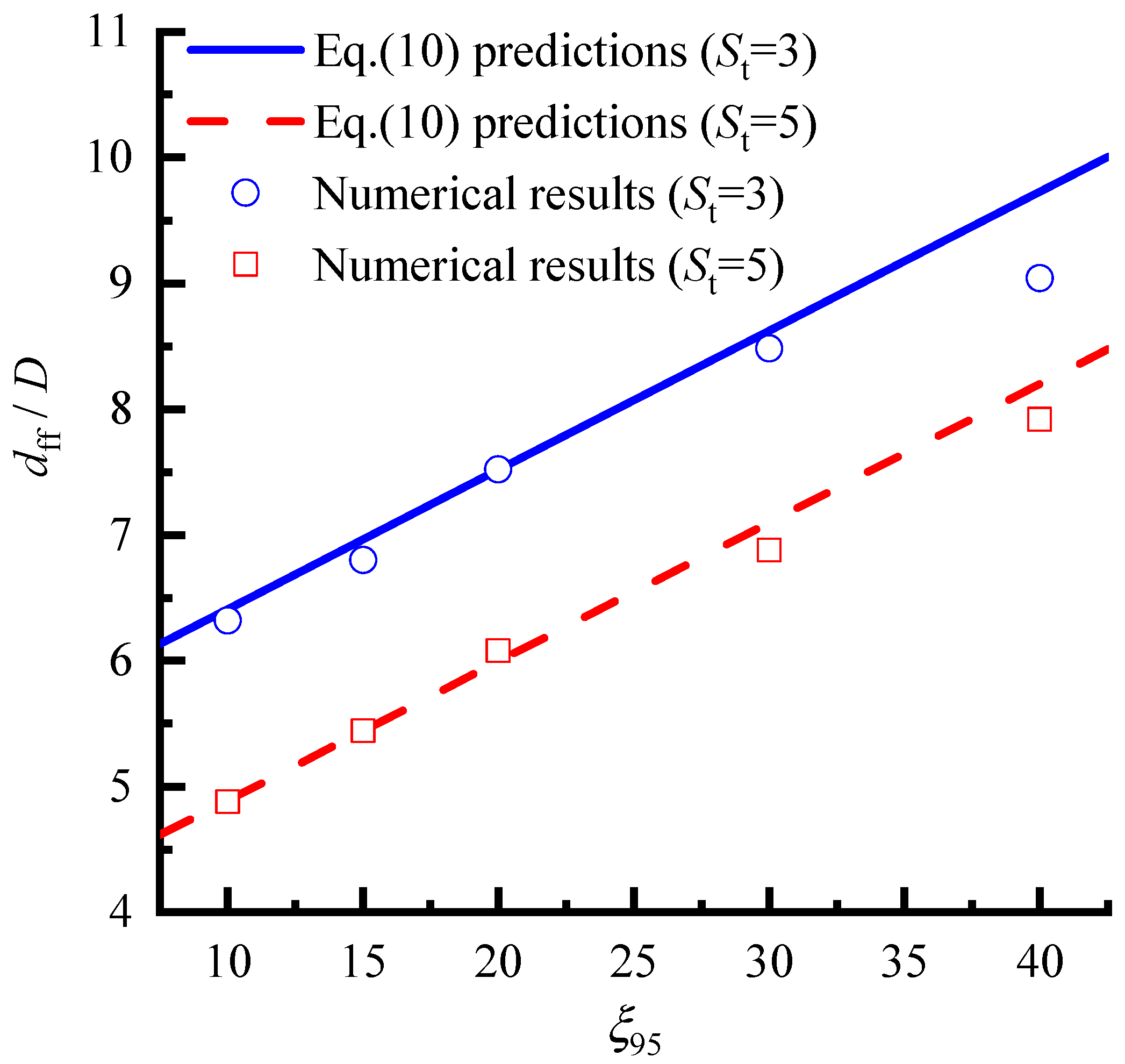
The influence of ξ₉₅ on the full-flow penetration depth d_ff/D is addressed in Figure 7. It can be observed that, for a given s_u/γ′D and S_t, the larger the ξ₉₅, the higher the critical depths of the soil. For instance, when s_u/γ′D = 3 and S_t = 3, the full-flow critical depth d_ff rises by 43% as ξ₉₅ varies from 10 to 40. Therefore, the influence of ductility-softening parameter ξ₉₅ on the critical depths should be considered.

It should be noted that Equations (10) and (11) are empirical in nature, derived from regression analyses of the numerical results. The selected variables are physically motivated by previous studies on T-bar penetration [1,8]. These expressions are applicable within the parameter ranges investigated in this study; extrapolation beyond these ranges should be made with caution.

4. Results of the Cyclic T-Bar Penetrations

The amplitude of the cycle and the minimum depth required for initiating the pull-out phase of the cyclic test (i.e., the depth at which the T-bar begins to move upward) are crucial for ensuring the consistency of resistance degradation curves obtained in a particular soil layer. In terms of cycle amplitude, theoretical solutions and numerical results indicate that a depth amplitude of 3D is necessary for ensuring that the soil at the midpoint of the cyclic range completely passes through the T-bar [2,17]. Shorter cyclic magnitudes can also eventually remold the soil strength, but additional cycles may be required to reach a stable resistance value at the midpoint of the cyclic range. This will result in the uncertainty of the value of N₉₅, which will affect the determination of softening parameters of soft soil. Therefore, an interval depth of 3D is adopted in this paper. Regarding the minimum depth required for initiating the pull-out stage of the cyclic test, previous cyclic tests were conducted at a fixed depth of 10D, which was considered sufficient to commence the pull-out process [7]. Numerical simulations have indicated that the minimum depth for initiating the pull-out phase of a cyclic test should exceed the full-flow depth d_ff, although no method was provided for determining this minimum depth [8].

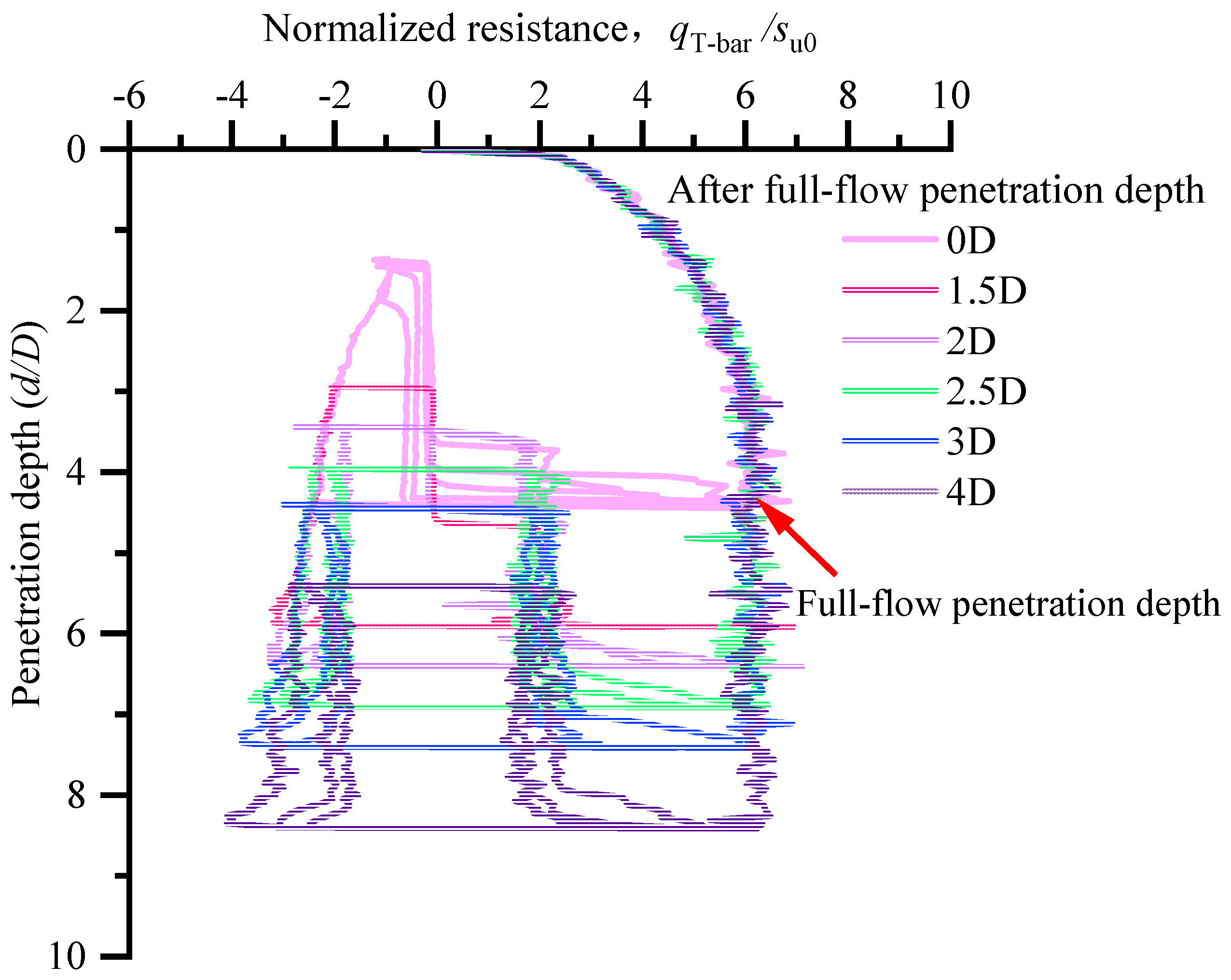
For the case of s_u/γ′D = 3, S_t = 10, and ξ₉₅ = 15, six depths, w_ext = 4.4D, 5.9D, 6.4D, 6.9D, 7.4D, and 8.4D (that is, 0, 1.5D, 2D, 2.5D, 3D, and 4D beneath the full-flow depth, respectively), were considered to investigate the influence of the minimum depth on the mechanism and resistance profile during cyclic test.

Figure 8 illustrates the six resistance profiles cycled at various depths in the clay. It is evident that, for the case of 0, 1.5D and 2D beneath the full-flow depth, the resistance exhibits a continuous decline during the first uplift stage, and remains nearly zero from the beginning to a certain depth in the second penetration stage before experiencing a sharp increase beyond that depth. Conversely, for the deep cyclic cases (2.5D, 3D, and 4D beneath the full-flow depth), the resistance is relatively stable around the midpoint of the cyclic range.

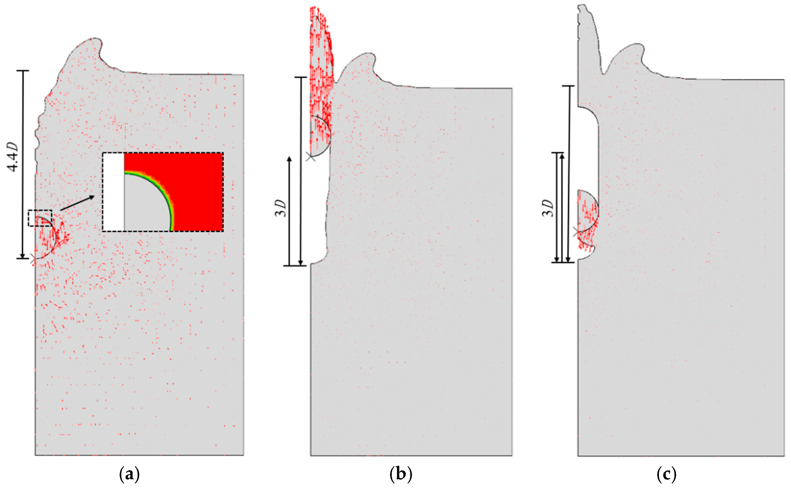
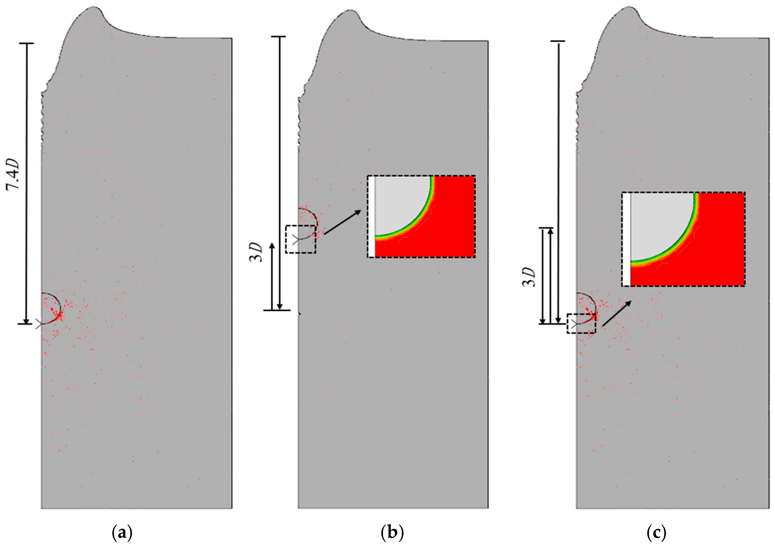
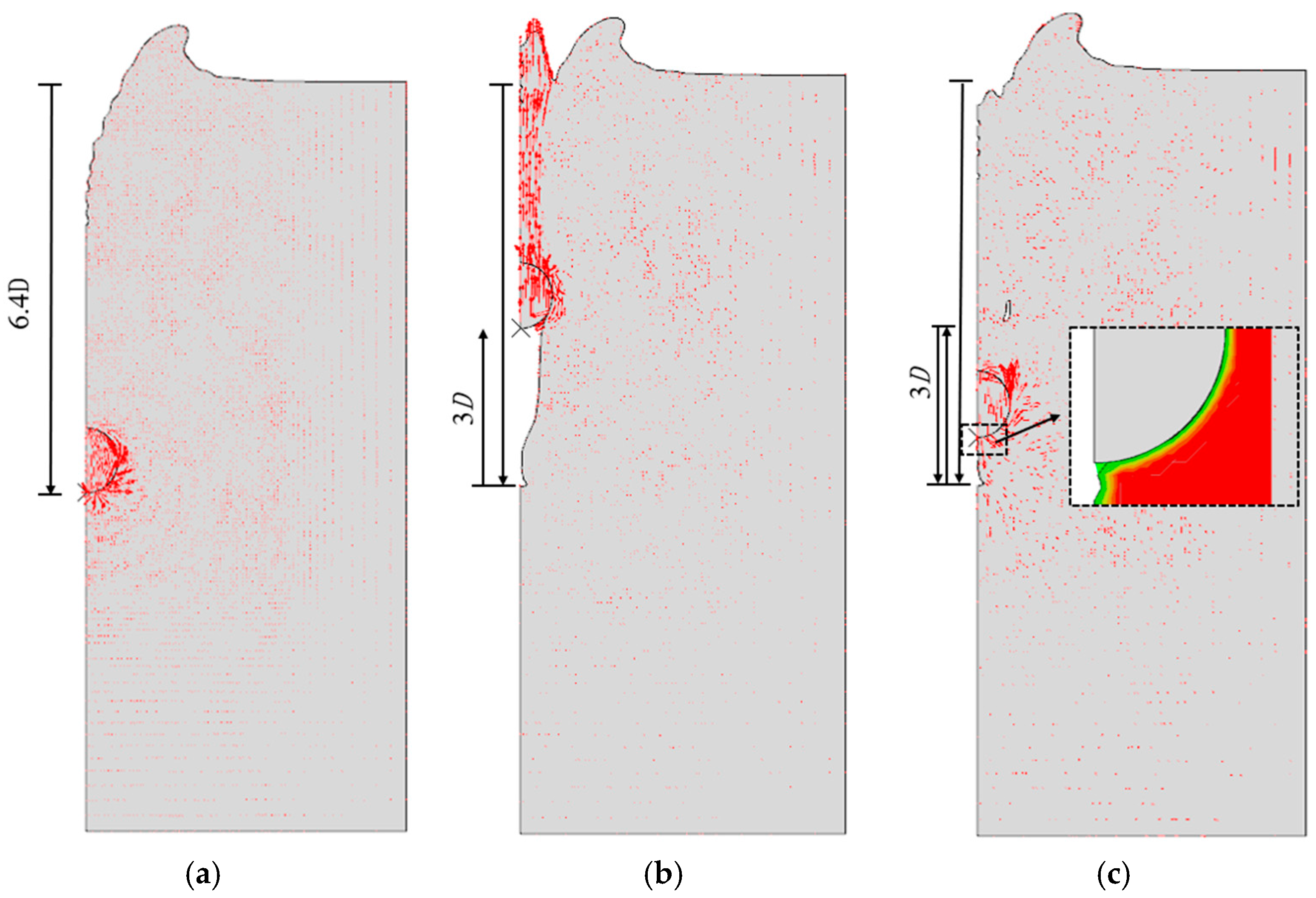
Figure 9, Figure 10 and Figure 11 show the flow mechanisms of cyclic cases of w_ext = 4.4D, 6.4D and 7.4D. For the shallow cyclic cases, there is a cavity behind the T-bar during the first extraction, as shown in Figure 9b and Figure 10b. Moreover, the cavity during uplift tends to be smaller when the depth w_ext, at which the T-bar begins to move upward, goes deeper. The flow mechanisms during the second penetration are illustrated in Figure 9c and Figure 10c. It can be observed that, in the course of the second penetration, a certain amount of soil on the side of the cavity is entrapped beneath the T-bar. The resistance is solely provided by the trapped soil. At the beginning of the second penetration stage, the volume of the trapped soil is relatively small, and thus the resistance is extremely low, as presented in Figure 9c and Figure 10c. With the increase in penetration depth, the distance between the trapped soil and the cavity bottom decreases. Once the entrapped soil comes into contact with the cavity bottom, the resistance immediately increases dramatically. As aforementioned, with the increasing depth w_ext, the smaller the cavity formed in the uplift stage, the greater the volume of soil trapped in the subsequent penetration, resulting in an earlier increase in resistance.

For the case of w_ext = 7.4D, as shown in Figure 11, the fully localized flow mechanism is mobilized during the entire cyclic penetration and extraction; therefore, the resistance profiles tend to be consistent with each other. It is evident that only the resistance profile acquired in this instance can be used to estimate the strain-softening parameters of soft clay.

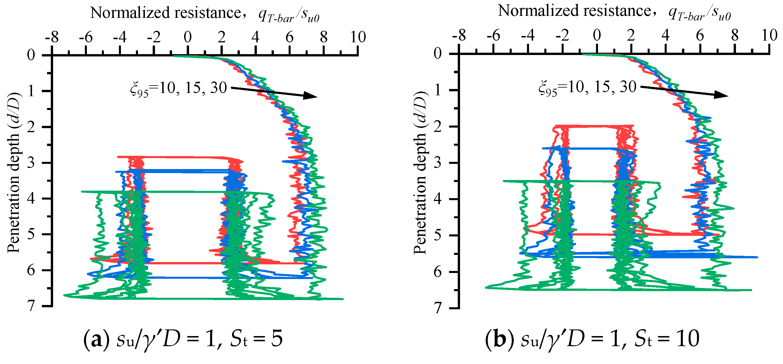
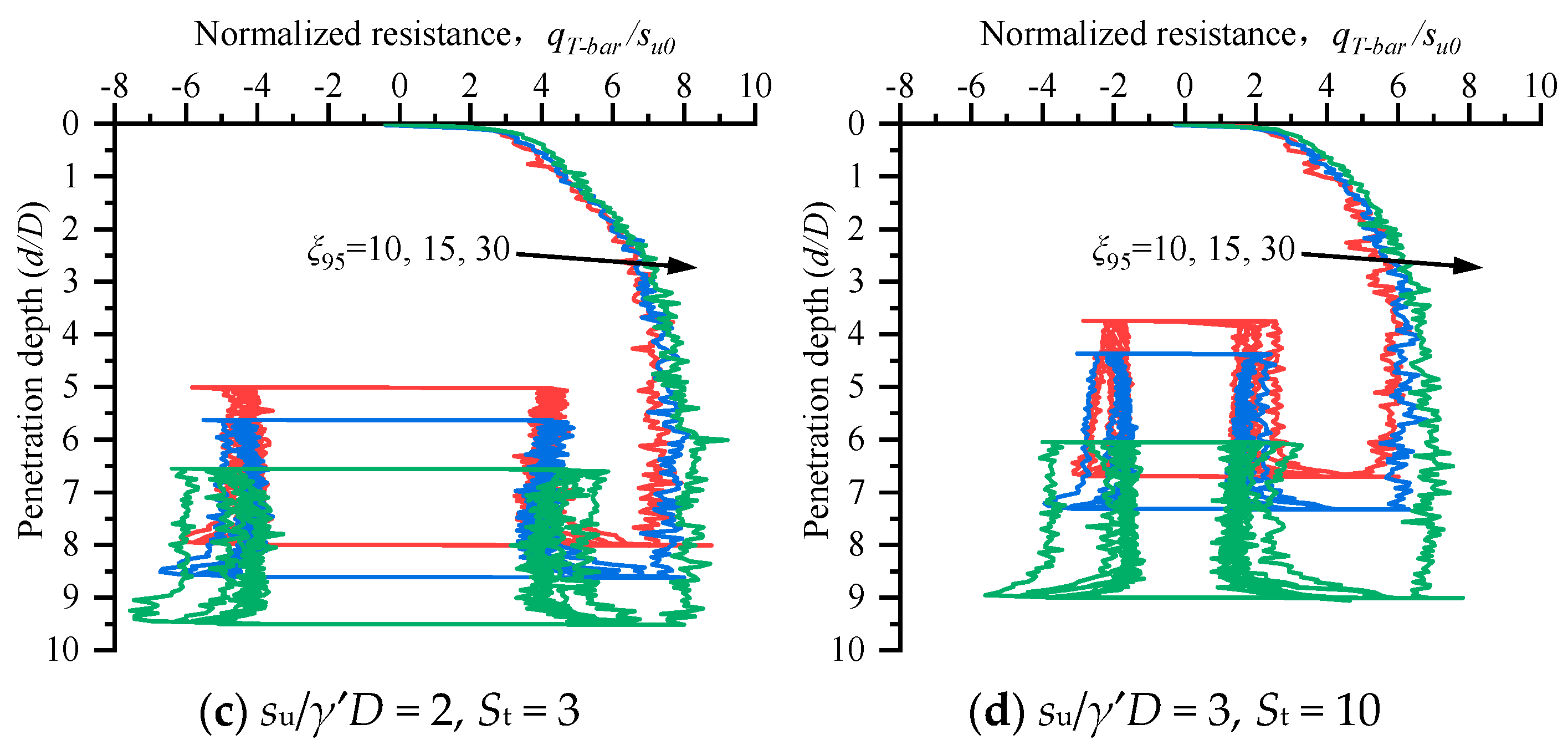
A similar approach is employed to investigate the cases with different strain-softening parameters listed in

Table 2. Summary of cyclic test simulations.

su/γ′D	St	ξ95
1	5	10/15/30
1	10	10/15/30
2	3	10/15/30
3	10	10/15/30

. The results indicate that the minimum depth necessary for initiating the pull-out phase of the cyclic test is d_s = d_ff + 3D. This criterion ensures that, considering the cyclic amplitude of 3D, the upper reversal point remains at or below d_ff throughout the pull-out phase, thereby guaranteeing a full-flow mechanism for all cases. Consequently, the resistance profiles obtained from cyclic tests initiated at various locations below this minimum depth are consistent, provided that the soil layer is adequately thick and uniform. The normalized resistance vs. penetration depth profiles for cases listed in Table 2 are shown in Figure 12.

5. Refined Resistance Degradation Model

Once the resistance profile is obtained, the strain-softening parameters of soft clay can be interpreted from the decay relation of resistances q_n with cycle numbers n. Some decay functions have been proposed to model the gradual degradation in resistance during cyclic tests. However, there is a defect in these models, which is that when the number of cycles reaches N₉₅, the model’s prediction does not achieve a 95% reduction in penetration resistance, as noted in the introduction. Based on an existing decay function for cyclic resistance degradation [19], a refined resistance degradation model is developed to overcome this shortcoming:

$${\displaystyle \frac{q_n}{q_{\mathrm{in}}}}={\displaystyle \frac{q_{\mathrm{rem}}}{q_{\mathrm{in}}}}+\left(1-{\displaystyle \frac{q_{\mathrm{rem}}}{q_{\mathrm{in}}}}\right){\mathrm{e}}^{-3{\left[\left(n-0.25\right)/\left(N_{95}-0.25\right)\right]}^{\beta }}$$

(12)

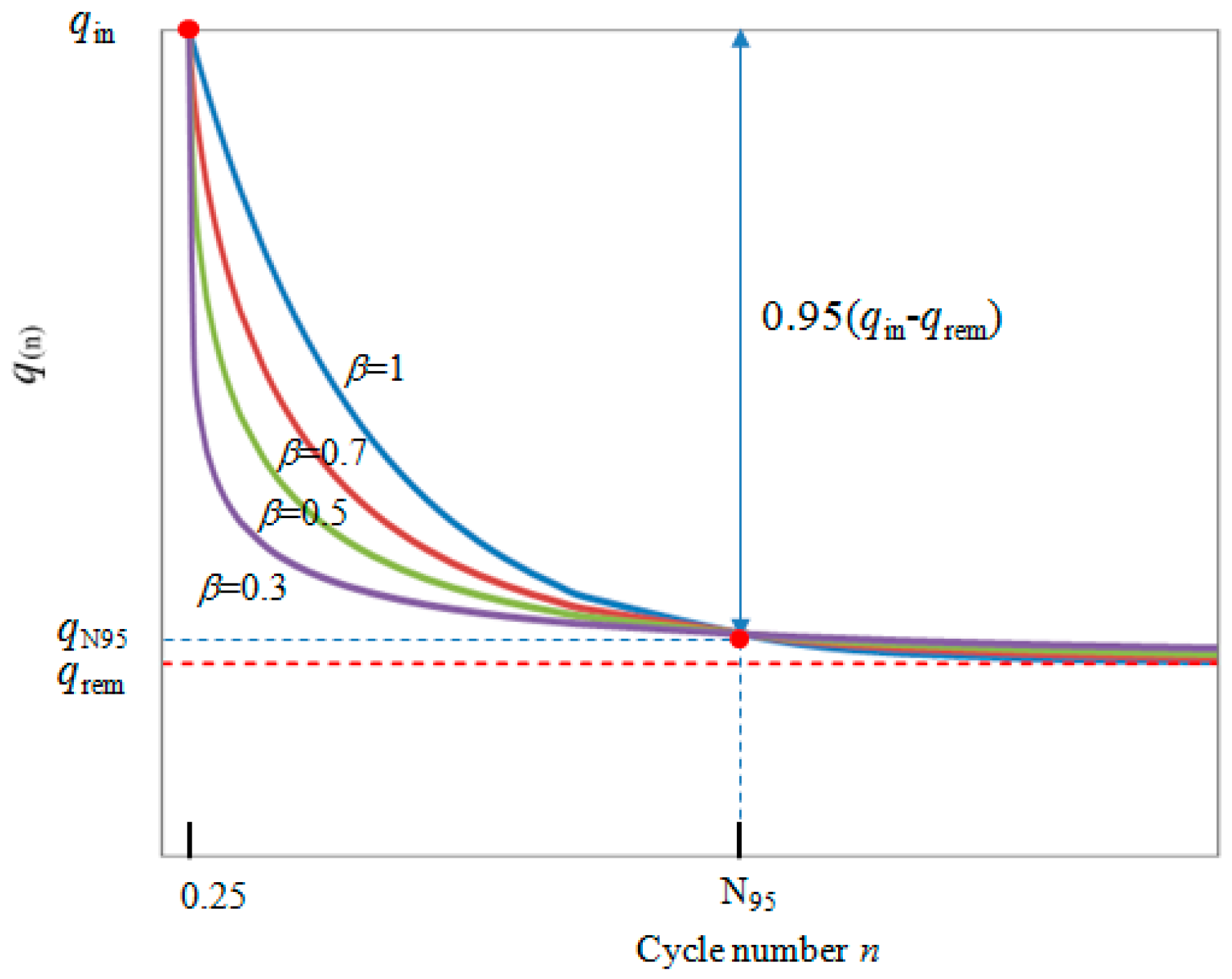
If $f\left(n\right){=\mathrm{e}}^{-3{\left[\left(n-0.25\right)/\left(N_{95}-0.25\right)\right]}^{\beta }}$, then the function f(n) always satisfies the three limiting conditions: f(0.25) = 1 (i.e., q_0.25/q_in = 1), f(∞) = 0, (i.e., q_∞/q_in = q_rem/q_in) and f(N₉₅) = 0.05 (i.e., ${\mathrm{e}}^{-3}=0.05$ and $q_{N_{95}}=q_{\mathrm{rem}}+0.05\left(q_{\mathrm{in}}-q_{\mathrm{rem}}\right)$). Figure 13 shows the general shape function of the refined model, emphasizing the limiting conditions (that is, a monotonic decrease from q_0.25 = q_in to q_∞ = q_rem, and a 95% reduction at N₉₅), as well as the influence of β on the slope of the function.

5.1. Estimation of N₉₅

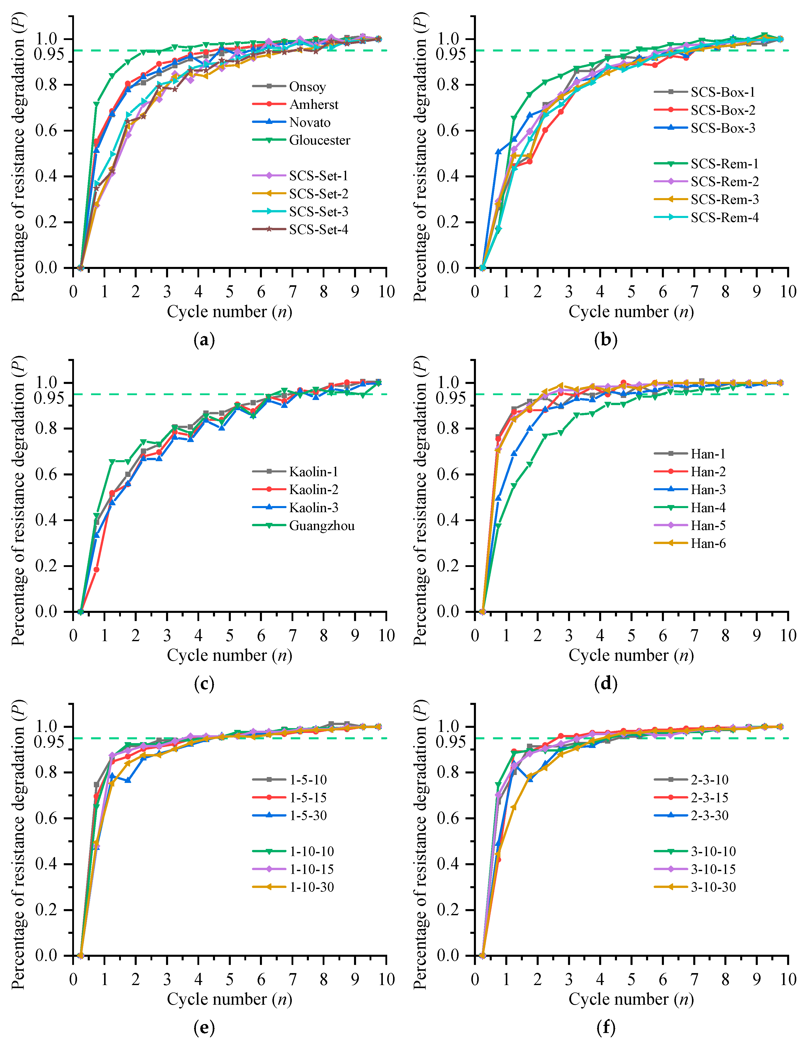
An existing method was employed to estimate N₉₅ [19]. Specifically, the relationship curve between the percentage of resistance degradation (P) and the cycle numbers (n) was first constructed, and subsequently, the horizontal coordinate of the point corresponding to the percentage of resistance degradation P = 95% on the curve was read. The percentage of resistance degradation is calculated as follows:

$$P={\displaystyle \frac{q_{\mathrm{in}}-q_n}{q_{\mathrm{in}}-q_{\mathrm{rem}}}}={\displaystyle \frac{1-q_n/q_{\mathrm{in}}}{1-q_{\mathrm{rem}}/q_{\mathrm{in}}}}\times 100\%$$

(13)

To comprehensively examine the performance of the refined resistance degradation model, the results of 37 different sets of physical or numerical tests were selected, and are listed in

Table 3. Summary of parameters of resistance degradation model for different test results.

Cases	qrem/ qin	qext/ qin	N95	${\mathit{N}}_{95}^{*}$	β	Reference
Onsøy	0.247	0.56	3.937	5.31	0.6	Yafrate et al. (2009) [15] Wang et al. (2018) [21] Ren et al. (2019) [22] Han et al. (2023) [23] Han et al. (2020) [8] This study
Amherst	0.169	0.57	3.527	4.71	0.65
Novato	0.238	0.51	3.542	5.44	0.55
Gloucester	0.055	0.33	1.553	3.00	0.51
SCS-Box-1	0.241	0.79	6.477	7.06	0.84
SCS-Box-2	0.200	0.86	6.962	7.37	0.95
SCS-Box-3	0.159	0.57	5.982	7.04	0.66
SCS-Set-1	0.044	0.74	5.212	6.28	0.91
SCS-Set-2	0.088	0.74	6.574	7.41	0.88
SCS-Set-3	0.063	0.65	5.775	6.29	0.81
SCS-Set-4	0.080	0.68	6.070	7.41	0.83
SCS-Rem-1	0.381	0.82	4.720	5.37	0.80
SCS-Rem-2	0.397	0.83	5.795	6.46	0.80
SCS-Rem-3	0.281	0.80	6.241	7.33	0.83
SCS-Rem-4	0.489	0.91	6.376	6.99	0.85
Kaolin-1	0.441	0.78	5.760	7.18	0.72
Kaolin-2	0.463	0.90	6.986	7.13	0.85
Kaolin-3	0.476	0.83	6.899	7.69	0.76
Guangzhou	0.486	0.79	6.186	6.39	0.71
Han-1	0.541	0.65	1.510	3.18	0.53
Han-2	0.543	0.66	2.260	2.71	0.54
Han-3	0.493	0.75	3.071	4.10	0.66
Han-4	0.490	0.81	5.127	5.86	0.73
Han-5	0.398	0.57	1.675	2.53	0.52
Han-6	0.237	0.46	1.680	2.18	0.51
1-5-10	0.362	0.52	1.441	3.65	0.50
1-5-15	0.343	0.54	2.176	4.06	0.52
1-5-30	0.329	0.68	3.763	4.47	0.67
1-10-10	0.233	0.50	1.545	4.05	0.55
1-10-15	0.213	0.62	2.140	3.15	0.68
1-10-30	0.187	0.60	3.606	4.43	0.67
2-3-10	0.514	0.67	1.728	4.57	0.57
2-3-15	0.507	0.79	1.936	2.38	0.70
2-3-30	0.469	0.74	3.750	4.18	0.66
3-10-10	0.254	0.44	1.402	4.26	0.48
3-10-15	0.230	0.46	1.811	3.33	0.51
3-10-30	0.199	0.64	3.493	4.06	0.70

. Among these datasets, apart from the 12 sets of numerical test data generated in this study, 19 sets were obtained from cyclic field tests at various locations [15,21,22,23] and six sets from previous numerical modeling data [8].

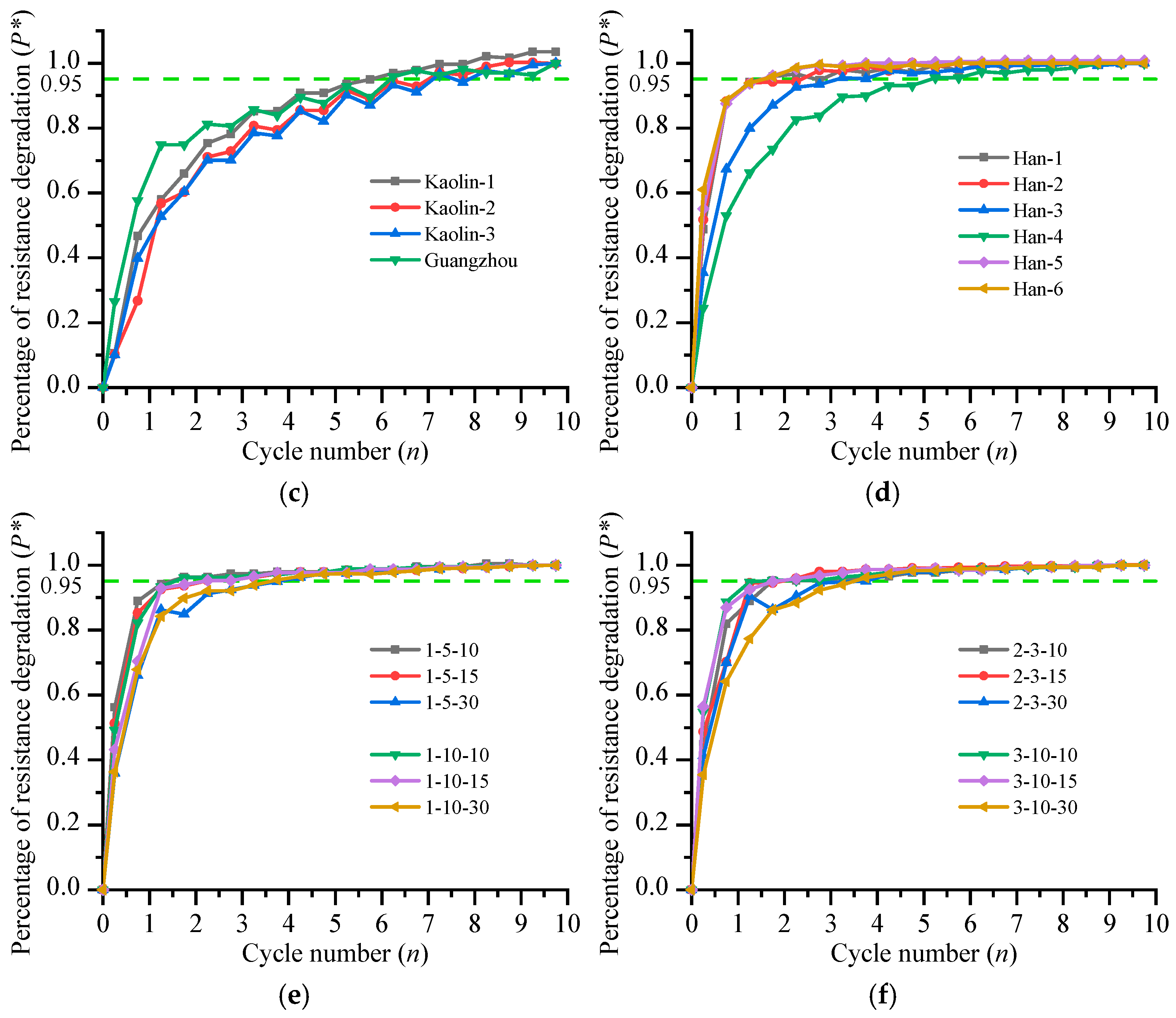
According to Equation (13), the percentage of resistance degradation P versus the number of cycles n for these 37 sets of tests is depicted in Figure 14. The horizontal lines indicate the resistance at 95% degradation. The values of N₉₅ predicted are listed in Table 3. It is noted that numerical test cases in this study are labeled following the convention “s_u/γ′D-S_t-ξ₉₅”. For instance, case “1-5-10” denotes the parameter set s_u/γ′D = 1, S_t = 5 and ξ₉₅ = 10.

5.2. Estimation of the Parameter β

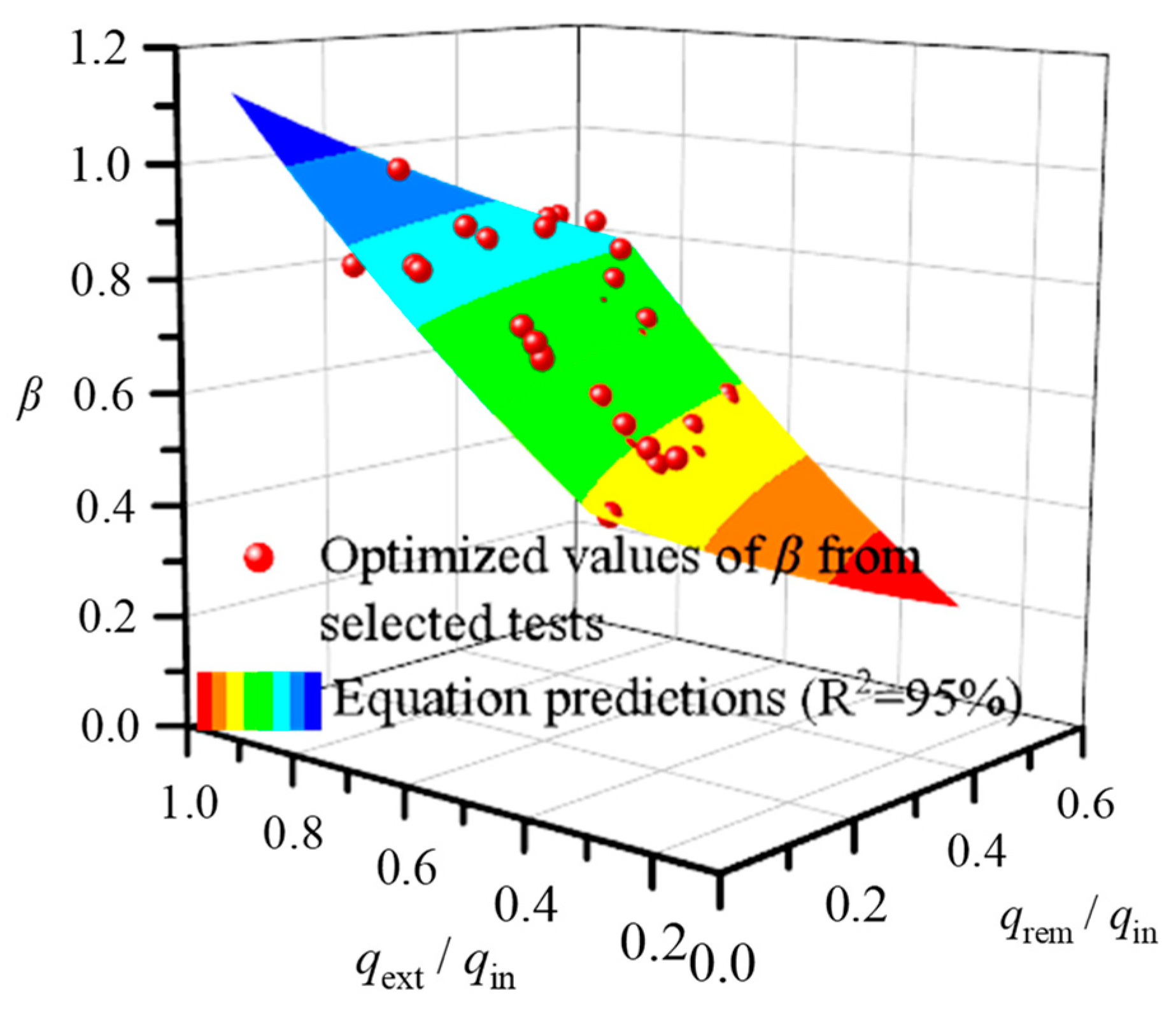
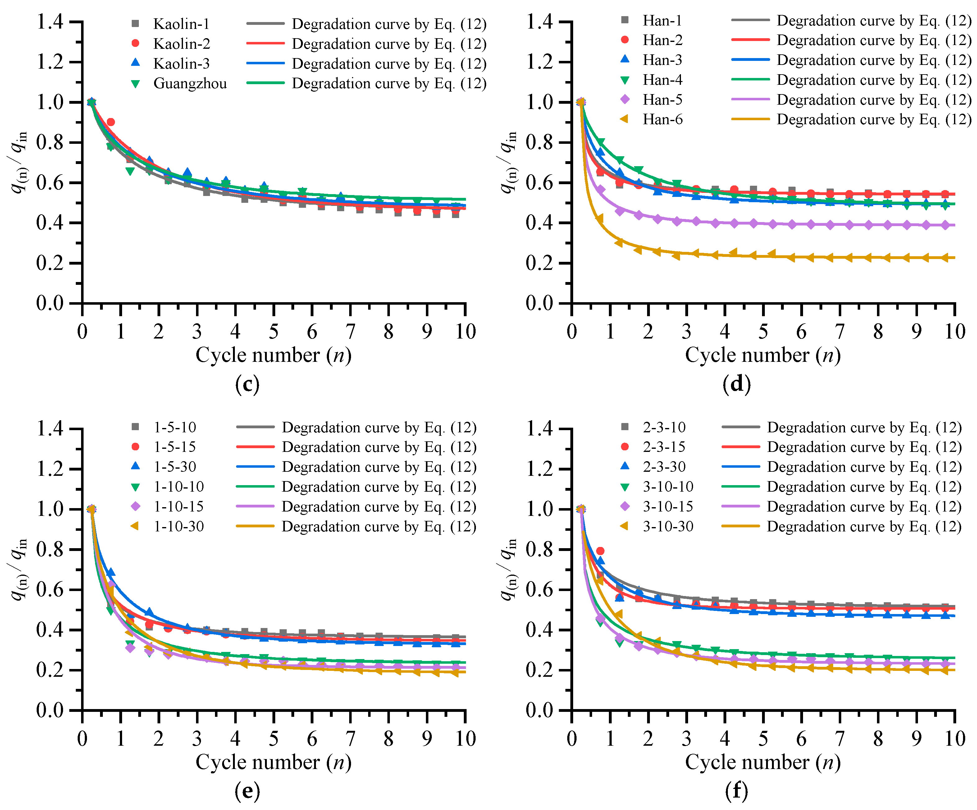
Once N₉₅ has been determined, the T-bar resistance degradation curve can be predicted by Equation (12) through optimizing the parameter β. The optimized values of β for each test result are shown in Figure 15. It is evident that the parameter β is dependent on the initial brittleness of soil and its fully remolded state. Therefore, based on the results of the 37 tests listed in Table 3, a relation was established to estimate β:

$$\beta ={0.49}^{{\displaystyle \frac{q_{\mathrm{rem}}}{q_{\mathrm{in}}}}}+{1.96}^{{\displaystyle \frac{q_{\mathrm{ext}}}{q_{\mathrm{in}}}}}-1.7$$

(14)

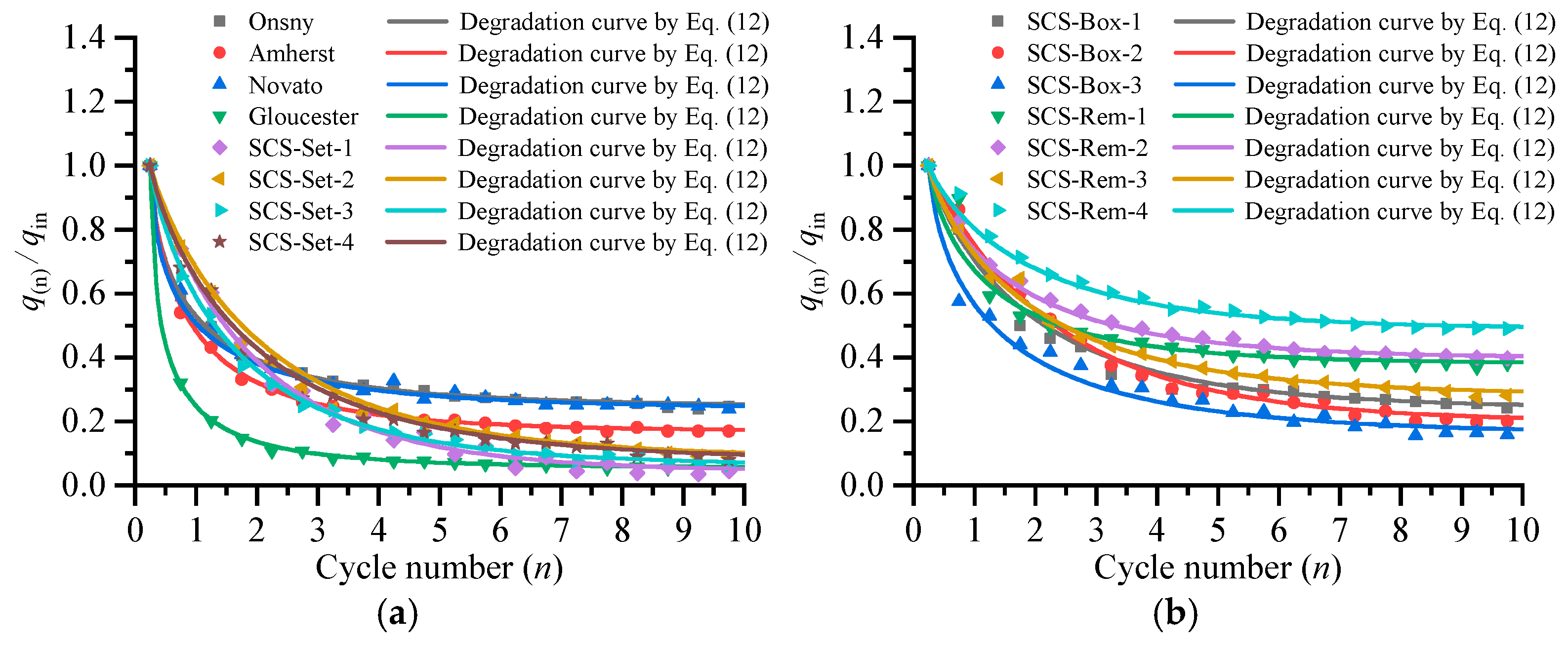
The values of β estimated using Equation (14) agreed well with the optimized values for each test. Based on these results, the parameters defining the refined resistance degradation model are presented in Table 3. Figure 16 compares the degradation curves predicted by Equation (12) with those directly derived from the selected tests. It can be observed that the refined resistance degradation model is in good agreement with all test results. It should be noted that the advantage of the proposed model over the previous formulation lies not only in fitting quality but more importantly in its theoretical consistency with the definition of N₉₅. The previous model, despite potentially achieving reasonable graphical agreement with test data, fails to correctly predict the degradation at n = N₉₅, which may lead to biased estimates of strain-softening parameters. Therefore, the present refinement addresses a fundamental theoretical deficiency rather than merely improving empirical curve-fitting.

6. Estimation of the Strain-Softening Parameters

The three parameters S_t (=1/δ_rem), ξ₉₅ and s_u0 in the strain-softening model are commonly used to characterize the intrinsic properties of marine clays [14]. The decay function of resistance can indicate the strain softening of soil to a certain extent; however, the value of q_in/q_rem is consistently lower than the sensitivity S_t of clay. Additionally, the approach of determining s_u0 by dividing the initial penetration resistance q_in by the constant bearing coefficient (typically 10.5) also suffers from the issue of underestimating the intact strength of the clay. This is because the T-bar penetrometer brings disturbance to the soil during the first penetration (n = 0.25), thereby making q_in (=q_0.25) not the penetration resistance of the soil in the intact state. Therefore, based on the refined resistance degradation model, an estimation method for strain-softening parameters of soft clay is developed.

6.1. Estimating Soil Sensitivity S_t

As stated above, the penetration resistance of intact soil (denoted by q_intact or q₀, as distinguished from q_in) cannot be actually measured using T-bar penetrometer tests. However, it can be extrapolated from Equation (12) by taking n = 0 [17], given by

$${\displaystyle \frac{q_{\mathrm{intact}}}{q_{\mathrm{in}}}}={\displaystyle \frac{q_{\mathrm{rem}}}{q_{\mathrm{in}}}}+\left(1-{\displaystyle \frac{q_{\mathrm{rem}}}{q_{\mathrm{in}}}}\right){\mathrm{e}}^{3{\left[0.25/\left(N_{95}-0.25\right)\right]}^{\beta }}$$

(15)

The soil sensitivity St is defined as follows [19]:

$$S_{\mathrm{t}}={\displaystyle \frac{s_{\mathrm{u}0}}{s_{\mathrm{ur}}}}={\displaystyle \frac{q_{\mathrm{intact}}}{q_{\mathrm{rem}}}}={\displaystyle \frac{q_{\mathrm{intact}}}{q_{\mathrm{in}}}}\times {\displaystyle \frac{q_{\mathrm{in}}}{q_{\mathrm{rem}}}}=\lambda {\displaystyle \frac{q_{\mathrm{in}}}{q_{\mathrm{rem}}}}$$

(16)

where s_ur is the fully remolded strength of soil and λ is the resistance ratio of q_intact/q_in.

It should be acknowledged that the estimation of q_intact relies on extrapolation of the resistance degradation curve because the T-bar has already disturbed the soil during its initial penetration. This extrapolation inevitably introduces some uncertainty, and the accuracy of the estimated intact resistance depends on the theoretical soundness of the resistance degradation model. The present refinement addresses this issue by ensuring consistency at N₉₅, thereby providing a more reliable basis for the extrapolation.

6.2. Estimating Ductility Parameter ξ₉₅

The ductility parameter ξ₉₅ can be calculated according to the following formula:

$${\xi }_{95}=2N_{95}^{\ast }{\xi }_{\mathrm{p}}$$

(17)

where $N_{95}^{\ast }$ represents the number of cycles required to reach 95% degradation from the theoretical intact value q_intact. This $N_{95}^{\ast }$ is different from the N₉₅ value, which is measured practically for a 95% degradation from the first penetration resistance q_in. ξ_p is the average magnitude of plastic shear strain undergone by soil elements passing through the failure mechanism in the individual penetration stage. The average plastic shear strain ξ_p can be estimated using the following expression [25]:

$${\xi }_{\mathrm{p}}=0.83\log S_{\mathrm{t}}+3.09$$

(18)

$N_{95}^{\ast }$ can be estimated through a method similar to that employed for N₉₅ [18]. The only difference lies in the fact that the relationship curve between the theoretical percentage of resistance degradation (P*) and the number of cycles needs to be established, and P* can be computed as follows:

$$P^{\ast }={\displaystyle \frac{q_{\mathrm{intact}}-q_n}{q_{\mathrm{intact}}-q_{\mathrm{rem}}}}={\displaystyle \frac{\lambda -q_n/q_{\mathrm{in}}}{\lambda -q_{\mathrm{rem}}/q_{\mathrm{in}}}}\times 100\%$$

(19)

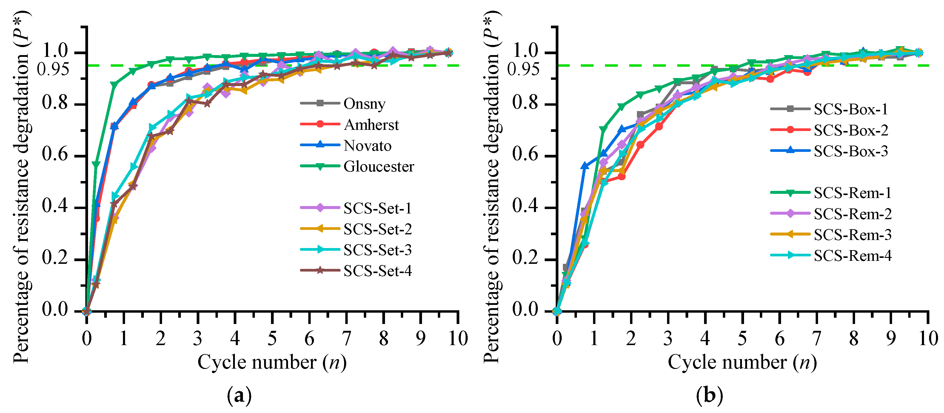
According to Equation (19), the theoretical resistance degradation percentage P* versus the number of cycles n for these 37 tests is depicted in Figure 17. The horizontal lines indicate the resistance at 95% degradation from the value q_intact. The predicted values of $N_{95}^{\ast }$ are listed in Table 3.

6.3. Estimating Intact Strength s_u0

According to the analyses mentioned above, the intact strength s_u0 can be estimated by the value of q_intact as

$$s_{\mathrm{u}0}={\displaystyle \frac{q_{\mathrm{intact}}}{N_{\mathrm{c}0}}}={\displaystyle \frac{\lambda q_{\mathrm{in}}}{N_{\mathrm{c}0}}}$$

(20)

where Nc0 is the bearing factor without strain softening.

For the T-bar, based on the exact closed-form solutions, the bearing factor N_c0 can be obtained as

$$N_{\mathrm{c}0}=\mathsf{\pi }+2\mathsf{\Delta }+2\cos \mathsf{\Delta }+4\left[\cos \left({\displaystyle \frac{\mathsf{\Delta }}{2}}\right)+\sin \left({\displaystyle \frac{\mathsf{\Delta }}{2}}\right)\right]$$

(21)

where Δ = sin⁻¹α, α is the friction ratio of the penetrometer, and α = δ_rem in this paper.

6.4. Verification

In this section, a series of T-bar cyclic tests are introduced to verify the reliability of the soil parameter estimation method.

6.4.1. Centrifuge Tests

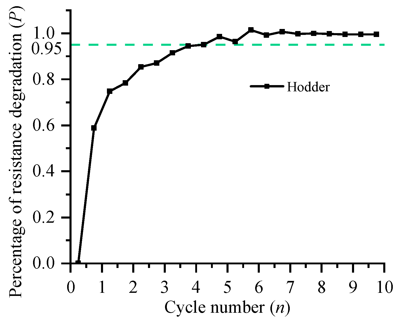
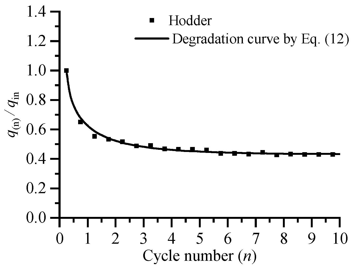
A centrifuge cyclic T-bar test was conducted in UWA kaolin clay [24]. The T-bar has a diameter of 25 cm in prototype. The cyclic resistance profile from the centrifuge test was used to deduce the strain-softening parameters of UWA kaolin clay following the proposed procedure [24]. Through drawing the curve of percentage of resistance degradation with cycle numbers, as shown in Figure 18, N₉₅ = 4.2 was obtained. The value of β was calculated to be 0.62 by substituting the corresponding data into Equation (14). Figure 19 illustrates the degradation curve predicted by Equation (12), as well as experimental data points from the centrifuge test [24]. As shown in Figure 19, the refined resistance degradation model exhibits excellent agreement with the experimental data points. Following the soil parameter estimation procedure, the derived strain-softening parameters are summarized in

Table 4. Strain-softening parameters from different methods.

N95	β	St	ξ95	Note
-	-	2.8	25	Hodder et al. (2010) [24]
-	-	2.38	25.6	Chen et al. (2021) [1]
4.2	0.64	3.2	24.8	Han et al. (2020) [19]
4.2	0.62	3.3	24.4	This study

. For comparison, Table 4 also includes parameters obtained from experimental measurements and those interpreted using existing methods [1,19,24]. An expression for the resistance-softening factor during initial penetration and a soil-parameter back-analysis framework based on a global search algorithm have been established in previous research [1]. Although the soil-parameter interpretation procedure proposed in this study has a form similar to an existing method, two critical distinctions exist: (i) the definition of N₉₅ in the existing resistance degradation model contains inherent limitations, as mentioned in the introduction; (ii) the exponent β as a constitutive model parameter is integrated into the soil strain-softening model, which unnecessarily increases the number of constitutive parameters. In contrast, the present method defines β exclusively as a parameter within the resistance degradation model to adjust the slope of the resistance degradation curve. This approach achieves superior fitting to cyclic resistance data points measured in cyclic tests while avoiding the introduction of redundant constitutive parameters, thereby enhancing the flexibility of the proposed method.

As evidenced by the comparative analysis in Table 4, the soil parameters derived using the proposed estimation method exhibit minimal discrepancies compared with those calculated using the existing method [19]. The sensitivity and ductility parameters obtained from the proposed method demonstrate a 17.9% increase and a 2.4% decrease, respectively, relative to the experimental results [24]. The existing back-analysis method predicted a 15% lower sensitivity and a 2.4% higher ductility parameter compared with the corresponding experimental data [1,24]. These comparisons indicate that, for the centrifuge test data, the parameter prediction accuracy of the proposed method is comparable to those of existing methods [1,8,19,24]. However, the refined resistance degradation model adopted in this study is theoretically justified, as its formulation satisfies the physical definition of N₉₅.

6.4.2. Field Tests

Cyclic T-bar tests, ball penetrometer tests, and field vane tests were performed at Onsøy, Norway, Amherst, United States, Novato, California and Gloucester, Canada [15]. The sensitivities of the four sites were determined using standard field vane tests (FVTs) with a vane radius of 32.5 mm and a rotation rate of 1°/min. A comparison between the sensitivities estimated by different resistance degradation models and the measured values from FVTs is presented in

Table 5. Sensitivities deduced from different models for Onsøy, Amherst, Novato and Gloucester.

Site	FVTs	Einav and Randolph (2005) [14]	Han et al. (2020) [19]	This Study
Onsøy	6	4.27	5.60	5.99
Amherst	8.5	6.44	8.84	8.80
Novato	6.5	4.73	5.69	6.53
Gloucester	68	23.72	43.45	42.64

. As shown in Table 5, the proposed method in this paper yields results closer to the measured values for the Onsøy, Amherst, and Novato sites. For instance, at the Novato site, the proposed method exhibits an error of only 0.5%, significantly lower than the 12.5% and 27% errors obtained from existing models [8,14,19]. Although the prediction accuracy of the proposed method for the Gloucester site is inferior to that of the existing method, both approaches show substantial deviations from the vane test measurements [8,19]. The underestimation may be attributed to three factors. First, the proposed method was calibrated primarily for soils with moderate sensitivity (typically S_t < 20); its direct extrapolation to highly sensitive clays (e.g., S_t = 68) inevitably introduces considerable uncertainty. Second, the field vane shear test itself may overestimate the in situ sensitivity in highly structured clays. Third, the cyclic T-bar-derived sensitivity represents a cyclic degradation parameter, which may not be fully equivalent to the field vane sensitivity measured under monotonic shearing conditions, especially for highly structured clays. Therefore, while the proposed method is most reliable for soils with S_t < 20, its application to extremely sensitive clays should be interpreted with caution.

6.4.3. Laboratory Tests

Laboratory cyclic T-bar tests on Speswhite kaolin clay and Guangzhou offshore clay were used to verify the proposed method in this section [23]. The cylindrical column samples were used to measure the soil strength degradation response. The diameter of the column is 110 mm, which is the same as the gravity-corer box sample. The mini T-bar has a diameter of D = 8 mm and a length of L = 40 mm. During cyclic T-bar testing, a velocity of 0.8 mm/s was applied to maintain undrained conditions. The softening parameters and intact strength estimated from the proposed method are shown in

Table 6. Comparison of proposed-method estimates with cyclic T-bar test data from [23].

Samples	su0/kPa	ξ95	St
Kaolin 1	6.35 (6.9)	39.67	2.67 (2.5)
Kaolin 2	5.62 (6.4)	47.56	2.39 (2.3)
Kaolin 3	3.96 (4.3)	46.95	2.38 (2.2)
Guangzhou	8.32 (7.9)	42.21	2.44 (2.2)

. The values in brackets in Table 6 were obtained from experimental measurements reported in the previous study [23]. By comparison, the proposed method is shown to provide reasonable estimates of strain-softening parameters for soft clay.

6.4.4. Numerical Tests

The proposed method is verified further by comparing the estimated values with the numerical test data from the current study. Based on the cyclic resistance degradation curves obtained from numerical experiments, the strength-related soil parameters were determined using the proposed estimation method and subsequently compared with the actual values (i.e., the known parameters input into the numerical model), as shown in

Table 7. Comparison of proposed-method estimates with numerical simulation input parameters from this study.

Numerical Tests	su0/kPa	ξ95	St
1-5-10	0.28 (0.24)	10.57 (10)	4.98 (5)
1-5-15	0.28 (0.24)	15.96 (15)	4.96 (5)
1-5-30	0.25 (0.24)	27.15 (30)	4.20 (5)
1-10-10	0.26 (0.24)	11.78 (10)	7.44 (10)
1-10-15	0.24 (0.24)	16.33 (15)	7.51 (10)
1-10-30	0.25 (0.24)	27.64 (30)	7.85 (10)
2-3-10	0.46 (0.48)	11.92 (10)	2.71 (3)
2-3-15	0.51 (0.48)	13.45 (15)	2.90 (3)
2-3-30	0.50 (0.48)	25.99 (30)	2.84 (3)
3-10-10	0.84 (0.72)	10.68 (10)	7.48 (10)
3-10-15	0.92 (0.72)	14.01 (15)	8.73 (10)
3-10-30	0.79 (0.72)	26.59 (30)	7.28 (10)

. The values in brackets in Table 7 were the actual parameters pre-defined in the CEL finite-element model.

As shown in Table 7, the difference between the estimated result and the corresponding actual value is acceptable. Comparing the estimated value of s_u0 with the actual value, the results show that the maximum error is 27.8% under s_u0/γ′D = 3, S_t = 10 and ξ₉₅ = 15 (i.e., 3-10-15). The error between the estimated value of ξ₉₅ and the actual value is no more than 20%. For the estimated value of S_t, the maximum error is 27.2% under s_u0/γ′D = 3, S_t = 10 and ξ₉₅ = 30. The comparison reveals that the proposed method for estimating the three softening parameters achieves accuracy within an acceptable range for engineering applications.

7. Conclusions

This study presented large-deformation finite-element (LDFE) simulations of cyclic T-bar penetration tests in soft clay. By implementing user-defined subroutines in ABAQUS/CEL, the numerical model incorporated the effects of soil strain-softening behavior for enhanced analysis accuracy.

During cyclic T-bar penetration and extraction, the flow mechanisms of the surrounding soil can be clearly observed. The trapped-cavity penetration depth (d_tc) and full-flow penetration depth (d_ff) were identified based on the trapped-cavity formation criterion and closure criterion respectively. Empirical equations for predicting these critical penetration depths, d_tc and d_ff, were proposed, accounting for both the amount and the rate of strength reduction of clay. These equations are applicable within the parameter ranges investigated in this study. The pull-out phase should initiate at depths exceeding d_ff + 3D (D is the diameter of the T-bar) to ensure full-flow mechanism activation in the surrounding soil throughout the cyclic test.

Moreover, a refined resistance degradation model is proposed, which corrects a defect in the existing model, which is that when the number of cycles is equal to N₉₅, the predicted result of the model does not reach 95% degradation in penetration resistance. A novel formulation for β is proposed to align with the refined degradation model. Then, an estimation method for strain-softening parameters of soft clay is developed. The method based on the refined resistance degradation model is verified by comparing the estimated values with the numerical simulation results and the available test data.

Several limitations of this study should be acknowledged. First, the proposed method was calibrated and validated primarily for soft clays with moderate sensitivity (S_t < 20); its extrapolation to highly sensitive clays should be made with caution. Second, the numerical analyses were conducted under undrained conditions, and consolidation effects during cyclic penetration were not considered. Third, the findings are based on T-bar penetrometers in soft clay; their applicability to other penetrometer types or to stiff soils requires further investigation. Addressing these limitations will form part of our future work.

References

1. Chen, X.; Han, C.; Liu, J.; Hu, Y. Interpreting strength parameters of strain-softening clay from shallow to deep embedment using ball and T-bar penetrometers. Comput. Geotech. 2021, 138, 104331. [Google Scholar] [CrossRef]
2. DeJong, J.; Yafrate, N.; DeGroot, D.; Low, H.E.; Randolph, M. Recommended Practice for Full-Flow Penetrometer Testing and Analysis. Geotech. Test. J. 2010, 33, 137–149. [Google Scholar] [CrossRef]
3. Chini, C.M.; Wallace, J.F.; Rutherford, C.J.; Peschel, J.M. Shearing Failure Visualization via Particle Tracking in Soft Clay Using a Transparent Soil. Geotech. Test. J. 2015, 38, 708–724. [Google Scholar] [CrossRef]
4. Puech, A.; Orozco-Calderón, M.; Foray, P. Mini T-bar testing at shallow penetration. In Frontiers in Offshore Geotechnics II; CRC Press: London, UK, 2010; pp. 305–310. [Google Scholar]
5. Westgate, Z.J.; White, D.J.; Randolph, M.F. Modelling the embedment process during offshore pipe-laying on fine-grained soils. Can. Geotech. J. 2013, 50, 15–27. [Google Scholar] [CrossRef]
6. Gaudin, C.; White, D.J. New centrifuge modelling techniques for investigating seabed pipeline behaviour. In Proceedings of the 17th International Conference on Soil Mechanics and Geotechnical Engineering, Alexandria, Egypt, 5–9 October 2009. [Google Scholar]
7. Zhou, H.; Randolph, M.F. Numerical investigations into cycling of full-flow penetrometers in soft clay. Géotechnique 2009, 59, 801–812. [Google Scholar] [CrossRef]
8. Han, Y.; Yu, L.; Yang, Q. Strain softening parameters estimation of soft clay by T-bar penetrometers. Appl. Ocean Res. 2020, 97, 102094. [Google Scholar] [CrossRef]
9. Tho, K.K.; Leung, C.F.; Chow, Y.K.; Palmer, A.C. Deep cavity flow mechanism of pipe penetration in clay. Can. Geotech. J. 2012, 49, 59–69. [Google Scholar] [CrossRef]
10. Wang, Y.; Hu, Y.; Hossain, M.S. Soil flow mechanisms of full-flow penetrometers in layered clays through particle image velocimetry analysis in centrifuge test. Can. Geotech. J. 2020, 57, 1719–1732. [Google Scholar] [CrossRef]
11. Wang, Y.; Hu, Y.; Hossain, M.S.; Zhou, M. Effect of Trapped Cavity Mechanism on Interpretation of T-Bar Penetrometer Data in Uniform Clay. J. Geotech. Geoenviron. Eng. 2020, 146, 04020078. [Google Scholar] [CrossRef]
12. White, D.J.; Gaudin, C.; Boylan, N.; Zhou, H. Interpretation of T-bar penetrometer tests at shallow embedment and in very soft soils. Can. Geotech. J. 2010, 47, 218–229. [Google Scholar] [CrossRef]
13. Zhou, M.; Hossain, M.S.; Hu, Y.; Liu, H. Behaviour of ball penetrometer in uniform single- and double-layer clays. Géotechnique 2013, 63, 682–694. [Google Scholar] [CrossRef]
14. Einav, I.; Randolph, M.F. Combining upper bound and strain path methods for evaluating penetration resistance. Int. J. Numer. Methods Eng. 2005, 63, 1991–2016. [Google Scholar] [CrossRef]
15. Yafrate, N.; DeJong, J.; DeGroot, D.; Randolph, M. Evaluation of Remolded Shear Strength and Sensitivity of Soft Clay Using Full-Flow Penetrometers. J. Geotech. Geoenviron. Eng. 2009, 135, 1179–1189. [Google Scholar] [CrossRef]
16. Zhou, H.; Randolph, M.F. Computational Techniques and Shear Band Development for Cylindrical and Spherical Penetrometers in Strain-Softening Clay. Int. J. Geomech. 2007, 7, 287–295. [Google Scholar] [CrossRef]
17. Zhou, H.; Randolph, M.F. Resistance of full-flow penetrometers in rate-dependent and strain-softening clay. Géotechnique 2009, 59, 79–86. [Google Scholar] [CrossRef]
18. Liu, J.; Chen, X.; Han, C.; Wang, X. Estimation of intact undrained shear strength of clay using full-flow penetrometers. Comput. Geotech. 2019, 115, 103161. [Google Scholar] [CrossRef]
19. Han, Y.; Yang, Q.; Yu, L.; Ren, Y. Optimized strain softening model for marine clay from cyclic full-flow penetration and extraction tests. Ocean Eng. 2020, 218, 108255. [Google Scholar] [CrossRef]
20. Hu, P.; Wang, D.; Cassidy, M.J.; Stanier, S.A. Predicting the resistance profile of a spudcan penetrating sand overlying clay. Can. Geotech. J. 2014, 51, 1151–1164. [Google Scholar] [CrossRef]
21. Wang, Y.; Ren, Y.; Yang, Q. Undrained Shear Strength Measurement for Deep-Sea Surficial Sediments in the West of South China Sea Using Miniature Full-Flow Penetrometer. In Proceedings of GeoShanghai 2018 International Conference: Fundamentals of Soil Behaviours; Springer: Singapore, 2018; pp. 371–378. [Google Scholar]
22. Ren, Y.; Yang, Q.; Wang, Y.; Zhao, W. Experimental study on the undrained shear strength of deep-sea soft soil using improved T-bar penetrometer. Mar. Georesources Geotechnol. 2019, 38, 1199–1208. [Google Scholar] [CrossRef]
23. Han, Y.; Yu, L.; Wang, Z.; Yang, Q.; Hu, Y. A novel T-bar test method ensuring full-flow mechanism in stiffer clay. Géotechnique 2023, 74, 1460–1474. [Google Scholar] [CrossRef]
24. Hodder, M.S.; White, D.J.; Cassidy, M.J. Analysis of Soil Strength Degradation during Episodes of Cyclic Loading, Illustrated by the T-Bar Penetration Test. Int. J. Geomech. 2010, 10, 117–123. [Google Scholar] [CrossRef]
25. Pinkert, S.; Klar, A. Enhanced Strain-Softening Model from Cyclic Full-Flow Penetration Tests. J. Geotech. Geoenviron. Eng. 2016, 142, 04015087. [Google Scholar] [CrossRef]
Figure 1. The failure mechanisms of the T-bar from shallow to deep penetration depths.
Jmse 14 01344 g001
Figure 2. CEL finite-element model of T-bar penetration.
Jmse 14 01344 g002
Figure 3. Comparison between the present results and previous numerical results reported in [17].
Jmse 14 01344 g003
Figure 4. Comparison between the present results and previous numerical results reported in [8].
Jmse 14 01344 g004
Figure 5. Instantaneous velocity vectors and cumulative plastic strain of the soil at various characteristic penetration depths (su/γD = 3, St = 3, and ξ95 = 15).
Jmse 14 01344 g005
Figure 6. Comparison between equation predictions and numerical simulation data for parametric cases with su/γD = 0.3–4.8, St = 2–20, and ξ95 = 10–40. (a) full-flow depth; (b) trapped-cavity depth.
Jmse 14 01344 g006
Figure 7. Effect of ξ95 on full-flow depth (su/γD = 3).
Jmse 14 01344 g007
Figure 8. Comparison diagram of normalized penetration resistance at different cycle starting points.
Jmse 14 01344 g008
Figure 9. The flow mechanism of soil for the cyclic T-bar test under wext = 4.4D. (a) the first penetration; (b) the first extraction; (c) the second penetration.
Jmse 14 01344 g009
Figure 10. The flow mechanism of soil for the cyclic T-bar test under wext = 6.4D. (a) the first penetration; (b) the first extraction; (c) the second penetration.
Jmse 14 01344 g010
Figure 11. The flow mechanism of soil for the cyclic T-bar test under wext = 7.4D. (a) the first penetration; (b) the first extraction; (c) the second penetration.
Jmse 14 01344 g011
Figure 12. Typical normalized resistance with the penetration depth under different strain-softening parameters (the red, blue, and green lines correspond to ξ95 = 10, 15 and 30, respectively). (a) su/γD = 1, St = 5; (b) su/γD = 1, St = 10; (c) su/γD = 2, St = 3; (d) su/γD = 3, St = 10.
Jmse 14 01344 g012aJmse 14 01344 g012b
Figure 13. The limiting conditions and the influence of β on the slope of the function in the refined model.
Jmse 14 01344 g013
Figure 14. Percentage of resistance degradation with cycle numbers. (a) field tests from [15,22]; (b) laboratory tests from [21,22]; (c) laboratory tests from [24]; (d) numerical tests from [8]; (e) numerical tests from this study; (f) numerical tests from this study.
Jmse 14 01344 g014
Figure 15. Optimized values vs. equation predictions.
Jmse 14 01344 g015
Figure 16. Model validation with normalized resistance from cyclic penetration tests in different soils. (a) field tests from [15,22]; (b) laboratory tests from [21,22]; (c) laboratory tests from [24]; (d) numerical tests from [8]; (e) numerical tests from this study; (f) numerical tests from this study.
Jmse 14 01344 g016aJmse 14 01344 g016b
Figure 17. Percentage of the theoretical resistance degradation with cycle numbers. (a) field tests from [15,22]; (b) laboratory tests from [21,22]; (c) laboratory tests from [24]; (d) numerical tests from [8]; (e) numerical tests from this study; (f) numerical tests from this study.
Jmse 14 01344 g017aJmse 14 01344 g017b
Figure 18. The curve of percentage of resistance degradation with cycle numbers reported in [24].
Jmse 14 01344 g018
Figure 19. The fitting results of Equation (12) and centrifuge test data reported in [24].
Jmse 14 01344 g019