Drivers of Coastal Water Quality and Ecological Status in the Bothnian Sea: Phosphorus Dynamics Across Scales

Abstract

Coastal water quality in the Bothnian Sea is shaped by interactions among local nutrient inputs, internal nutrient cycling, and basin-scale phosphorus enrichment, complicating the assessment and management of eutrophication. This study analyses long-term time series of nutrients (total phosphorus (TP), dissolved inorganic phosphorus (DIP), dissolved inorganic nitrogen (DIN), and total nitrogen (TN)) and phytoplankton indicators (chlorophyll a and biomass) from contrasting Finnish coastal systems off Uusikaupunki and Rauma. Despite higher external phosphorus loading in Rauma, nutrient concentrations and phytoplankton biomass remain lower than in the semi-enclosed Uusikaupunki coastal zone. In contrast, Uusikaupunki exhibits higher chlorophyll a concentrations and lower TP:Chl a ratios, suggesting greater phosphorus bioavailability. At the offshore station SR5, TP and DIP increase below the surface layer, while surface concentrations show no significant trends, indicating phosphorus accumulation in deeper waters. Declining DIN:DIP ratios indicate a shift toward nitrogen limitation, under which primary production increasingly depends on phosphorus-supported nitrogen fixation. Chlorophyll a increases across the coastal gradient, including the outer archipelago, indicating a spatial expansion of eutrophication. Together, these findings are consistent with a system-level shift toward phosphorus-driven production. The results demonstrate a dual-control system in which basin-scale phosphorus enrichment determines long-term background conditions, while local nutrient loading and legacy effects regulate spatial variability in ecosystem response. More broadly, the findings highlight the importance of cross-scale interactions between regional nutrient enrichment and local ecosystem processes for understanding and managing eutrophication in inland and semi-enclosed marine systems.

1. Introduction

Eutrophication is one of the major ecological pressures affecting inland and semi-enclosed seas worldwide, where restricted water exchange, strong stratification, and long water residence times often amplify the effects of external nutrient inputs. In these systems, internal nutrient cycling and sediment–water interactions can sustain elevated nutrient concentrations and delay ecosystem recovery even after reductions in external loading. As a result, eutrophication dynamics are often governed by interacting external inputs, internal feedback mechanisms, and large-scale physical forcing, leading to complex and non-linear ecosystem responses [1,2].

The Baltic Sea exemplifies many of these characteristics but is further distinguished by pronounced spatial heterogeneity and hydrodynamic variability. The relative importance of nutrient inputs, internal processes, and large-scale transport varies across spatial and temporal scales, particularly in the Finnish coastal zone, where hydrodynamic conditions and catchment characteristics differ substantially among coastal systems. Understanding how phosphorus dynamics emerge from the interaction of these processes is essential for assessing ecological status and developing effective management strategies.

Long-term studies have shown that internal ecosystem feedbacks can sustain high primary production even when external nutrient inputs are reduced. In particular, sediment phosphorus release combined with enhanced nitrogen fixation may maintain elevated phytoplankton biomass, thereby weakening the direct relationship between external nutrient loading and ecological response [3]. These feedback mechanisms contribute to the persistence of eutrophic conditions, especially in stratified coastal environments.

Simultaneously, large-scale background forcing has intensified during recent decades. Basin-scale analyses indicate increasing nutrient concentrations and transport within the Baltic Sea, particularly during winter, reflecting both climatic influences and long-term nutrient loading trends [4]. Recent modelling studies further suggest that phosphorus transport from the Baltic Proper to the Bothnian Sea has increased substantially since the early 2000s, resulting in elevated concentrations of dissolved inorganic phosphorus (DIP) in offshore waters [5]. These changes indicate an expansion of the offshore phosphorus reservoir and increased phosphorus availability. Such large-scale changes are increasingly recognized as a dominant control on nutrient dynamics in the Baltic Sea, where internally sustained phosphorus inputs can outweigh reductions in external loading [6,7].

The ecological significance of this development depends not only on total nutrient concentrations but also on the vertical distribution of phosphorus. In stratified Baltic Sea waters, DIP is typically depleted from surface layers during the productive season through biological uptake, while accumulating in intermediate and deep waters through remineralization and sediment-related processes. This separation between surface consumption and subsurface accumulation prolongs phosphorus residence times and strengthens internal nutrient cycling [3,4]. However, the extent to which offshore phosphorus accumulation influences coastal eutrophication through vertical and horizontal transport pathways remains poorly quantified.

Despite increasing background nutrient concentrations, pronounced coastal–offshore gradients in nutrient levels and phytoplankton biomass persist, indicating that local nutrient inputs and hydrodynamic conditions continue to exert strong ecological control [8,9]. Chlorophyll a, a widely used indicator of phytoplankton biomass and eutrophication status, integrates the effects of nutrient availability and internal biogeochemical processes and therefore provides a direct measure of ecosystem response [10]. Such gradients are a characteristic feature of Baltic coastal systems and arise from the interaction between local land-based nutrient inputs, hydrodynamic exchange processes regulating nutrient retention and dilution, and basin-scale nutrient forcing that sets the background nutrient availability.

Hydrodynamic conditions play a key role in modulating these responses. In relatively open coastal systems, efficient water exchange can limit nutrient accumulation and phytoplankton growth despite substantial external loading. Conversely, semi-enclosed coastal areas with restricted exchange are more susceptible to nutrient retention, enhanced internal loading, and persistent eutrophication [11]. Vertical exchange processes may further strengthen these effects by transporting phosphorus-rich deep waters into the euphotic zone, thereby stimulating primary production [5,12].

Previous studies have emphasized that ecological status in coastal waters is primarily determined by absolute nutrient and chlorophyll concentrations rather than temporal trends alone [8,11]. Consequently, increasing background phosphorus concentrations may elevate baseline nutrient availability and enhance ecosystem sensitivity to both local nutrient inputs and internal feedback mechanisms. At the same time, changes in nutrient stoichiometry—particularly declining DIN:DIP ratios—reflect shifts in nutrient limitation and are known to favor nitrogen-fixing cyanobacteria, thereby linking phosphorus enrichment to changes in phytoplankton community composition and ecosystem functioning [13]. These developments indicate a system-level response in which increasing phosphorus availability modifies nutrient limitation patterns and promotes a transition toward phosphorus-driven production.

In this study, long-term monitoring data for total phosphorus (TP), dissolved inorganic phosphorus (DIP), dissolved inorganic nitrogen (DIN), total nitrogen (TN), and phytoplankton indicators (chlorophyll a and biomass) were analyzed to disentangle the relative roles of local nutrient inputs, internal nutrient cycling, and basin-scale forcing in the Finnish coastal zone of the Bothnian Sea. The analysis is based on long-term monitoring data spanning multiple decades, with the longest time series extending from the 1960s to 2025, thereby covering both the period prior to and following the increase in phosphorus transport from the Baltic Proper observed since the early 2000s.

The study areas were selected primarily based on the availability of long-term monitoring data and contrasting nutrient loading histories. In addition, the systems differ qualitatively in their hydrodynamic properties, with the semi-enclosed Uusikaupunki coastal area exhibiting more restricted water exchange compared to the more open and exposed Rauma coastal zone. By combining long-term time-series analyses with spatial comparisons and offshore–coastal linkages, the study examines how phosphorus dynamics across depth layers and spatial scales influence coastal water quality and ecological status.

These dynamics suggest a dual-control mechanism, in which basin-scale nutrient forcing sets the background conditions while local processes regulate the magnitude and spatial expression of coastal eutrophication. Specifically, the study addresses the hypothesis that recent deterioration of environmental conditions in the Bothnian Sea cannot be explained solely by local nutrient loading but reflects basin-scale phosphorus enrichment interacting with internal nutrient cycling, which modifies nutrient limitation patterns and amplifies ecological responses to local inputs. By quantifying the combined influence of basin-scale forcing, internal processes, and local loading, this study provides new insights into the mechanisms driving coastal eutrophication and their implications for future management of Baltic Sea coastal waters.

2. Material and Methods

2.1. Study Area

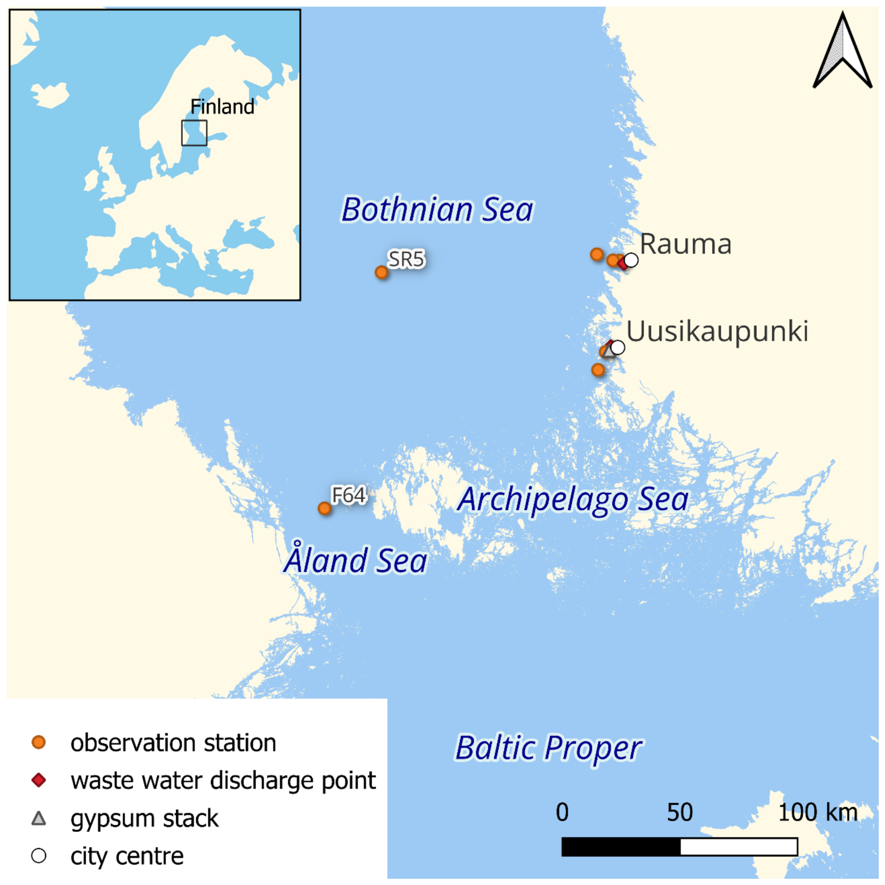
The Bothnian Sea forms the southern sub-basin of the Gulf of Bothnia in the northern Baltic Sea, located between the coasts of Finland and Sweden (Figure 1). It is bounded in the south by the Archipelago Sea and the Åland Sea, which together form a transition zone regulating water and nutrient exchange between the Baltic Proper and the Gulf of Bothnia [14,15].

The basin extends northwards to the Northern Quark (Kvarken), which separates it from the Bothnian Bay. The Bothnian Sea reaches maximum depths close to 300 m, particularly near the Swedish coast, although a large proportion of the basin is considerably shallower [16].

Hydrographically, the Bothnian Sea is a brackish basin with relatively low salinity, typically around 5–6 PSU in surface waters. The limited inflow of saline deep water from the Baltic Proper, constrained by the topography of the Åland region and basin geometry, has historically reduced the transport of nutrient-rich deep water into the Bothnian Sea. As a result, the basin has been less affected by eutrophication than southern Baltic sub-basins, although increasing riverine nutrient inputs are gradually altering this balance [17].

Water exchange between the Baltic Proper and the Bothnian Sea occurs primarily through the Archipelago Sea and the Åland Sea. This exchange is characterized by a two-layer circulation system, where saline inflows enter at depths below approximately 40 m, while fresher surface waters flow southwards. Model results indicate substantial annual transport volumes, with inflows to the Bothnian Sea on the order of several hundred cubic kilometers per year, accompanied by significant phosphorus fluxes that have increased in recent decades [5].

The Åland Sea, where one of the monitoring stations (F64) is located, forms a deep intermediary basin between the Baltic Proper and the Bothnian Sea. It is situated between the Swedish coast and the Åland Islands and has a mean depth of approximately 75 m, with a deep trench exceeding 300 m. Constrictions and sills within this basin regulate deep-water inflows and make it a key control point for saltwater and nutrient transport to the Bothnian Sea [14,18].

The coastal areas of Rauma and Uusikaupunki represent relatively open inner archipelago environments along the eastern Bothnian Sea coast, but with differing hydromorphological and hydrodynamic characteristics.

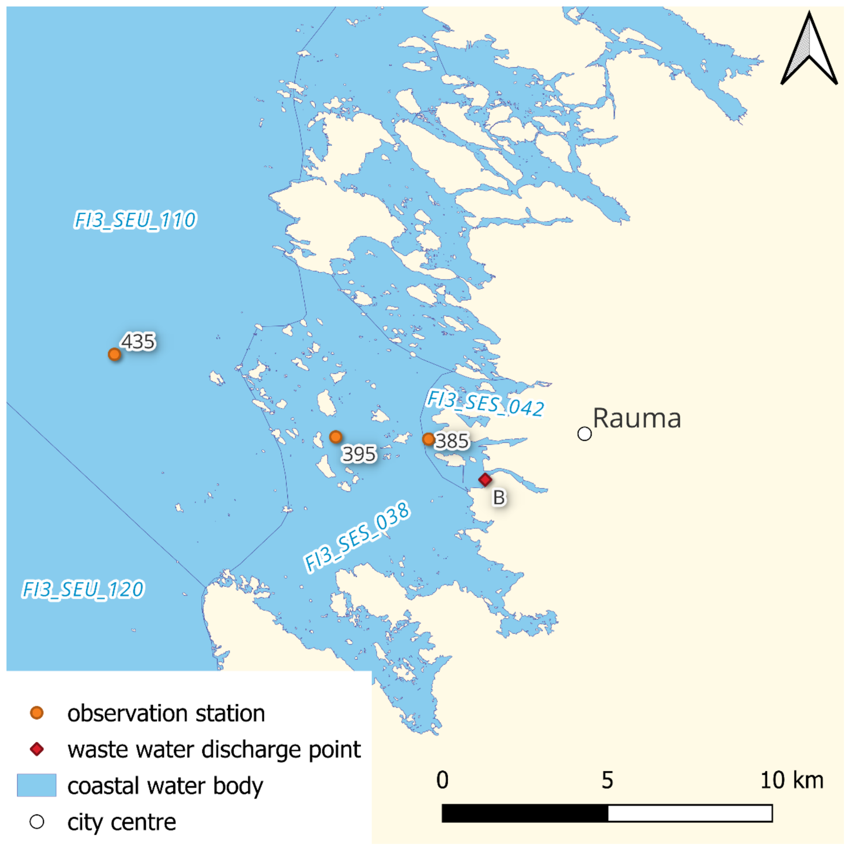
The Rauma coastal area is characterized by a narrow archipelago zone with mean water depths of approximately 5–7 m and maximum depths up to 15 m (Figure 2) [19]. Due to the limited extent of the archipelago, the influence of the open sea is pronounced even close to the shoreline. Water exchange is relatively efficient during the ice-free season, and circulation is dominated by a slow northward coastal current, accompanied by local bidirectional flows through deeper channels within the archipelago. Wind forcing, particularly easterly winds, can induce offshore surface transport and rapid renewal of the water mass through upwelling of deeper waters. Freshwater inputs are minor, and consequently diffuse nutrient loading from the catchment is low.

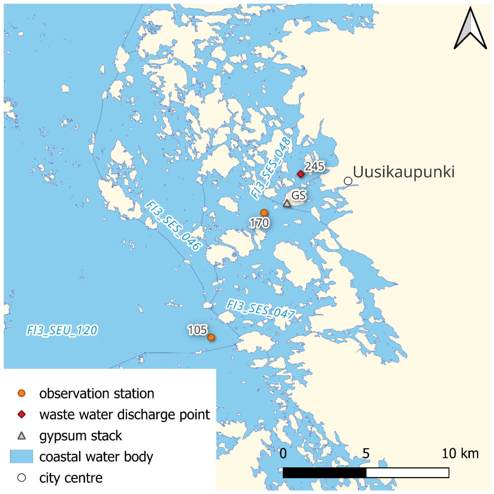
In contrast, the Uusikaupunki coastal area consists of a more extensive inner and middle archipelago, covering approximately 81 km², including about 35 km² of inner archipelago waters (Figure 3) [20]. The mean depth is approximately 7 m, with maximum depths ranging between 20 and 35 m. Hydrodynamic conditions are strongly influenced by the Sirppujoki River and an artificial freshwater basin (37 km²) constructed at its mouth, located north of the coastal water body FI3_SES_048. The Sirppujoki River discharges into an artificial freshwater basin, which buffers short-term variations in river flow and modifies the timing and magnitude of nutrient transport to the coastal area. As a result, this system significantly influences local circulation patterns and water quality.

The extensive archipelago structure and freshwater influence generally limit water exchange and increase retention compared to more open coastal systems, although these characteristics are described qualitatively rather than based on directly comparable quantitative metrics.

While phosphorus inputs from the river are retained within the basin due to precipitation under acidic conditions, the outflowing water is enriched in inorganic nitrogen, which can periodically elevate nitrogen concentrations in the adjacent coastal waters.

2.2. Nutrient Loading History, Rauma

Phosphorus (P) and nitrogen (N) loading in the Rauma coastal area show distinct temporal patterns over the period 1995–2024 (Table S1). Phosphorus loading increased from 8.8 t yr⁻¹ in 1995–1999 to 13.1 t yr⁻¹ in 2000–2004 and further to a peak of 16.2 t yr⁻¹ in 2005–2009. During the same period, BOD7 levels showed only moderate variation. After 2010, phosphorus loading decreased, reaching 4.7 t yr⁻¹ in 2024.

In contrast, nitrogen loading shows a more gradual and consistent decline over the study period, decreasing from approximately 190 t yr⁻¹ in the late 1990s to about 100–110 t yr⁻¹ in recent years.

The development of nutrient loading reflects changes in wastewater treatment practices, including the introduction of joint municipal and industrial treatment in 2002 and subsequent improvements in treatment performance over time.

2.3. Nutrient Loading History, Uusikaupunki

Nutrient loading from the freshwater basin to the Uusikaupunki sea area over the period 2011–2025 is characterized by pronounced interannual variability without a consistent long-term trend (Table S2).

Total nitrogen (N) loading ranged between 110.1 and 476.8 t yr⁻¹ during the study period. Elevated values were observed in several years (e.g., 2012, 2015, 2019, 2020, and 2023), whereas lower values occurred in 2014 and 2017. In recent years, nitrogen loading has remained moderate but variable.

Phosphorus (P) loading followed a similar pattern, ranging from 0.51 to 3.8 t yr⁻¹. Most years were characterized by phosphorus loads between approximately 0.8 and 2.6 t yr⁻¹, with higher values observed in 2020 and 2024. After the 2024 maximum, phosphorus loading decreased to 2.0 t yr⁻¹ in 2025.

Source apportionment for 2024 shows that the freshwater basin represents the dominant nutrient source to the Uusikaupunki sea area, contributing approximately 83% of total nitrogen and 69% of total phosphorus inputs. Other sources, including municipal wastewater, industrial effluents, fish farming, atmospheric deposition, and the gypsum stack area, contribute smaller shares.

These data indicate that nutrient loading from the freshwater basin constitutes the principal component of total nutrient inputs to the Uusikaupunki sea area, with pronounced interannual variability. The available time series reflects recent conditions under elevated basin-scale phosphorus levels rather than a directly comparable long-term loading record. A longer historical perspective is provided in the Supplementary Materials (Section S1), which documents the evolution of point-source phosphorus loading from the gypsum stack and associated legacy effects since the 1960s [21]. For context, in the Baltic Sea, areal sediment phosphorus inventories generally range from a few g m⁻² in low-accumulation systems to several tens of g m⁻² in coastal depositional areas [22,23]. Long-term accumulation and mobile or reactive phosphorus pools are typically only a few g m⁻² over decadal scales under oxic conditions [23,24]. Substantially higher inventories occur in eutrophic, high-loading environments, where organic matter deposition and redox-driven retention enhance phosphorus accumulation [12,25].

2.4. Water Quality Analytics and Data

Water quality in the Åland Sea and Bothnian Sea has been monitored for several decades, with the earliest measurements dating to the 1960s. The resulting measurements are publicly accessible through the Finnish Environment Institute’s VESLA platform (https://www.syke.fi/en/environmental-data/maps-and-information-services/open-environmental-information-systems, accessed 15 June 2026) including dissolved inorganic nitrogen (DIN) and dissolved inorganic phosphorus (DIP) concentrations used in this study. VESLA compiles physico-chemical data from nationwide and regional monitoring programs coordinated by environmental authorities, supplemented by statutory assessments performed by private entities and water protection organizations.

Methods for quantifying inorganic nutrients in marine environments are well established [26]. Although analytical methods and laboratory techniques have evolved over the monitoring period, they have been harmonized within national monitoring programs to ensure long-term comparability, and the large-scale trends and spatial patterns analyzed in this study are robust to such methodological changes.

In this study, the dataset is based on measurements conducted in accredited laboratories [27]. Typically, nutrient measurements were performed on unfiltered samples within 5–8 h of collection, with adjustments made for turbidity and color interference. Total phosphorus was determined following acidic digestion with K₂S₂O₈ and subsequent spectrophotometric detection as an ammonium molybdate blue complex [28]. Chlorophyll-a concentrations were assessed spectrophotometrically from ethanol extracts of samples filtered through Whatman GF/F filters (nominal pore size 0.7 µm) [29].

Phytoplankton were analyzed from composite production-layer samples collected in July–August, with layer depth defined as twice the Secchi depth. Samples were obtained using a 2 m tube sampler, with subsamples integrated evenly across the layer.

Species-level biomass and cell counts were determined following standard guidelines [30] using the Utermöhl method [31,32] and inverted microscopy. Phytoplankton analyses included major taxonomic groups such as cyanobacteria, dinoflagellates, flagellates, and Mesodinium rubrum (marine samples), with particular focus on cyanobacteria in the present study. Samples were settled in chambers of known area and quantified microscopically (units L⁻¹) using guideline conversion factors [30]. Biomass (wet weight) was calculated from biovolume assuming a density of 1 g cm⁻³ [32].

Ecological status of coastal waters was assessed in accordance with the EU Water Framework Directive using nationally defined classification criteria [33]. Summer chlorophyll-a, representing phytoplankton biomass, was applied as the primary indicator of eutrophication, with type-specific class boundaries defining ecological status. This approach follows the WFD framework, in which biological response variables form the basis of classification, while physico-chemical elements are used to support and verify the assessment. In the Bothnian Sea, chlorophyll-a provides a robust indicator of eutrophication because phosphorus concentrations during the productive season are rapidly assimilated and often approach detection limits, whereas phytoplankton biomass responds directly to nutrient availability in this predominantly P-limited system [3,4,13].

Total phosphorus and total nitrogen were used as supporting physico-chemical elements to ensure consistency between nutrient conditions and biological response. Ecological status classes (high, good, moderate, poor, bad) reflect deviations from reference conditions and were integrated following the national assessment framework applied in the fourth river basin management cycle.

Analyses were primarily conducted for the summer ecological classification period (1 July–7 September), as defined in national guidelines [33], representing conditions during the productive season. In addition, winter (1 January–31 March) concentrations of dissolved inorganic nitrogen (DIN) and dissolved inorganic phosphorus (DIP) were used to characterize nutrient availability under fully mixed conditions prior to the onset of biological uptake. Winter nutrient concentrations are widely applied indicators of eutrophication status and represent the pre-bloom nutrient pool controlling primary production in the subsequent growing season [34,35].

The use of wintertime total nitrogen concentrations provides a robust basis for assessing wastewater impacts, as hydrological and biogeochemical conditions during winter minimize biological variability and allow anthropogenic nutrient inputs to be detected more directly. During winter, the water column is typically fully mixed, ensuring comparability between coastal and offshore stations. At the same time, low temperatures and limited light suppress phytoplankton uptake, and nutrient dynamics are governed primarily by physical transport processes such as mixing and dilution [36]. Nitrogen is less affected by particle interactions and redox-dependent processes than phosphorus, making it more suitable for resolving spatial concentration gradients under well-mixed winter conditions.

Under these conditions, differences in nitrogen concentrations between coastal and offshore stations reflect gradients driven by external loading rather than internal ecosystem processes. In this study, the effects of multi-source nutrient loading off Uusikaupunki—originating from riverine inputs via a freshwater basin, wastewater discharges, and seepage from gypsum stacks—as well as wastewater inputs from Rauma were evaluated along a coastal–offshore concentration gradient using wintertime total nitrogen levels.

In contrast, summer nutrient concentrations are more strongly influenced by stratification and biological uptake, which can obscure the signal of external loading and limit their interpretability. For this reason, chlorophyll-a concentration serves not only as the primary classification variable but also as a complementary, process-based indicator during the productive season, integrating the effects of nutrient availability on phytoplankton biomass and primary production. Chlorophyll a is widely applied as a core indicator of eutrophication and ecological status in coastal and marine systems, including the Baltic Sea [37,38].

2.5. Calculations and Statistical Analysis

The nitrogen flux from the Baltic Proper to the Bothnian Sea was estimated by combining modeled volume transports with observed total nitrogen (TN) concentrations derived from monitoring data at station F64. Total nitrogen concentrations used in the calculations were obtained from monitoring data at station F64, representing inflowing water from the Baltic Proper.

The volume transports were adopted from Helminen and Inkala [5], who quantified water exchange across predefined transects using precomputed ocean circulation fields obtained from the Copernicus Marine Service regional reanalysis. These circulation fields and their configuration are described in detail by Helminen and Inkala [39]. They are based on the NEMO 4.0 ocean model and integrate satellite-derived sea surface temperature observations, in situ temperature and salinity profiles, and ERA5 atmospheric forcing. The reanalysis is configured at approximately 2 km horizontal resolution with 110 vertical z levels, with enhanced resolution in the upper layers, and includes realistic representations of river inflows, sea ice dynamics, and data assimilation of key hydrographic variables. Prognostic variables include three-dimensional velocity, temperature, salinity, and sea level, among others [39].

Volume fluxes were calculated by integrating modeled velocity fields across selected transects separating the Baltic Proper, Åland Sea, Archipelago Sea, and Bothnian Sea. Time series of water volume transport were constructed for each transect and subsequently aggregated into monthly net transports (km³), with positive and negative values indicating northward and southward flow, respectively.

Following the approach applied for phosphorus fluxes in Helminen and Inkala [5], the nitrogen fluxes were computed by multiplying the modeled volume transports (Q, km³ time⁻¹) by representative TN concentrations (C, µg L⁻¹) for each period:

F_N = Q × C

where F_N is the nitrogen flux. Seasonal and annual fluxes were derived from the monthly estimates.

Total nitrogen concentrations used in the calculations were obtained from monitoring data at station F64, representing inflowing water from the Baltic Proper. The selection of concentration data followed the same procedure as described for total phosphorus in Helminen and Inkala [5], ensuring consistency between nutrient flux estimates. No vertical differentiation in nitrogen concentrations was applied; instead, depth-integrated concentrations representative of the inflow were used in combination with layer-specific volume transports where applicable. This approach assumes that station F64 adequately characterizes the nutrient content of the water masses entering the Åland Sea from the Baltic Proper and that temporal variability in concentrations is captured by the monitoring dataset. Thus, station F64 is used to characterize basin-scale inflow conditions rather than to directly explain local coastal responses, consistent with the multi-scale framework applied in this study.

Statistical analyses were performed using Microsoft^® Excel^® for Microsoft 365 MSO (Version 2502 Build 16.0.18526.20264) and Python (https://www.python.org, accessed on 1 July 2026) (SciPy, NumPy, and Pandas libraries) [40].

Annual nutrient fluxes and concentrations were calculated from monthly or higher-frequency observations as arithmetic means or integrated annual sums, depending on data availability. Seasonal values were computed using the predefined summer and winter periods described above.

Long-term trends in nutrient fluxes and concentrations were quantified using ordinary least squares (OLS) linear regression, from which slope estimates (rate of change per year) and coefficients of determination (R²) were derived. The statistical significance of trends was evaluated based on regression p-values. To ensure robustness against non-normality and potential outliers, non-parametric Mann–Kendall tests were additionally applied, and Theil–Sen slope estimators were calculated as a complementary measure of trend magnitude [41,42,43].

Relationships between variables, including nutrient fluxes and modeled water exchange, were assessed using Pearson’s correlation coefficient (r). The significance of correlations was evaluated at the same significance level as for other statistical tests.

Differences between time periods (≤2010 vs. >2010) were tested using two-sample t-tests. In cases where data did not meet the assumptions of normality, the non-parametric Mann–Whitney U test was applied. Normality of residuals and data distributions was assessed visually.

Annual mean winter TN concentrations were calculated for each station prior to statistical analysis to ensure comparability among stations with different sampling frequencies.

Differences among stations were assessed using the Kruskal–Wallis test, a non-parametric alternative to one-way ANOVA that does not assume normality. Effect size for the Kruskal–Wallis test was estimated using epsilon-squared (ε²).

Pairwise differences between stations were evaluated using Welch’s t-test, which does not assume equal variances between groups. To account for multiple comparisons, p-values were adjusted using the Holm correction method.

LOWESS smoothing was applied using a fixed fraction (0.3) to illustrate long-term patterns while preserving interannual variability. In addition, 5-year centered moving averages were applied to selected time series for consistency across comparable variables. To facilitate interpretation of the figures, smoothed lines are used to highlight medium- to long-term patterns, while annual values represent underlying variability. Visual trends should therefore be interpreted in conjunction with statistical analyses reported in the text.

Statistical significance was assessed at α = 0.05.

3. Results

3.1. Nitrogen Flux from the Baltic Proper

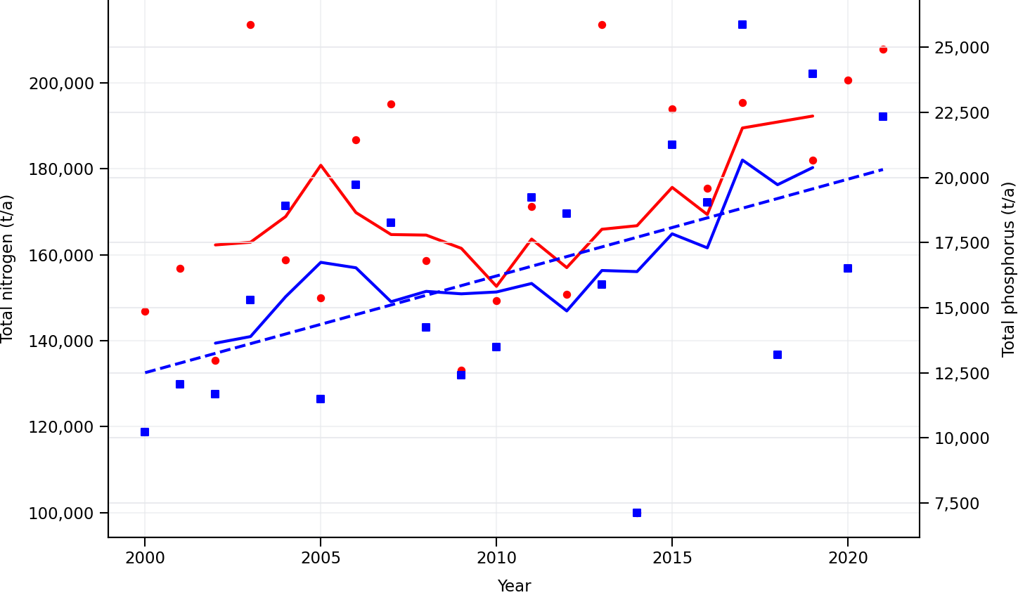
Annual nitrogen flux from the Baltic Proper to the Bothnian Sea during 2000–2021 ranged from approximately 1.0 × 10⁵ to 2.1 × 10⁵ t a⁻¹, indicating strong interannual variability (Figure 4). A weak increasing tendency (≈1.7 kt a⁻¹) was observed; however, the trend was not statistically significant due to substantial year-to-year fluctuations.

Nitrogen flux variability closely followed variations in modeled water exchange, with a very strong positive correlation (r ≈ 0.94), indicating that interannual variability in nitrogen transport was primarily controlled by hydrodynamic forcing rather than changes in nutrient concentrations.

Seasonal analysis showed that summer exchange remained relatively stable throughout the study period, whereas wintertime exchange exhibited indications of enhanced transport after approximately 2010. Consequently, the modest increase in annual nitrogen flux appears to be associated with intensified winter circulation. However, the difference between the earlier (≤2010) and later (>2010) periods was not statistically significant (p > 0.05), indicating that the apparent increase reflects high interannual variability rather than a systematic shift in circulation dynamics.

No statistically significant long-term trends were detected in nitrogen concentrations in either season. Summer concentrations remained stable, while winter concentrations were stable or showed a slight, non-significant decrease. These results indicate that both the variability and the weak increasing tendency in nitrogen flux were primarily driven by changes in physical transport rather than by changes in nutrient concentrations.

3.2. Contrasting Long-Term Trends in Winter DIN and DIP at Station SR5

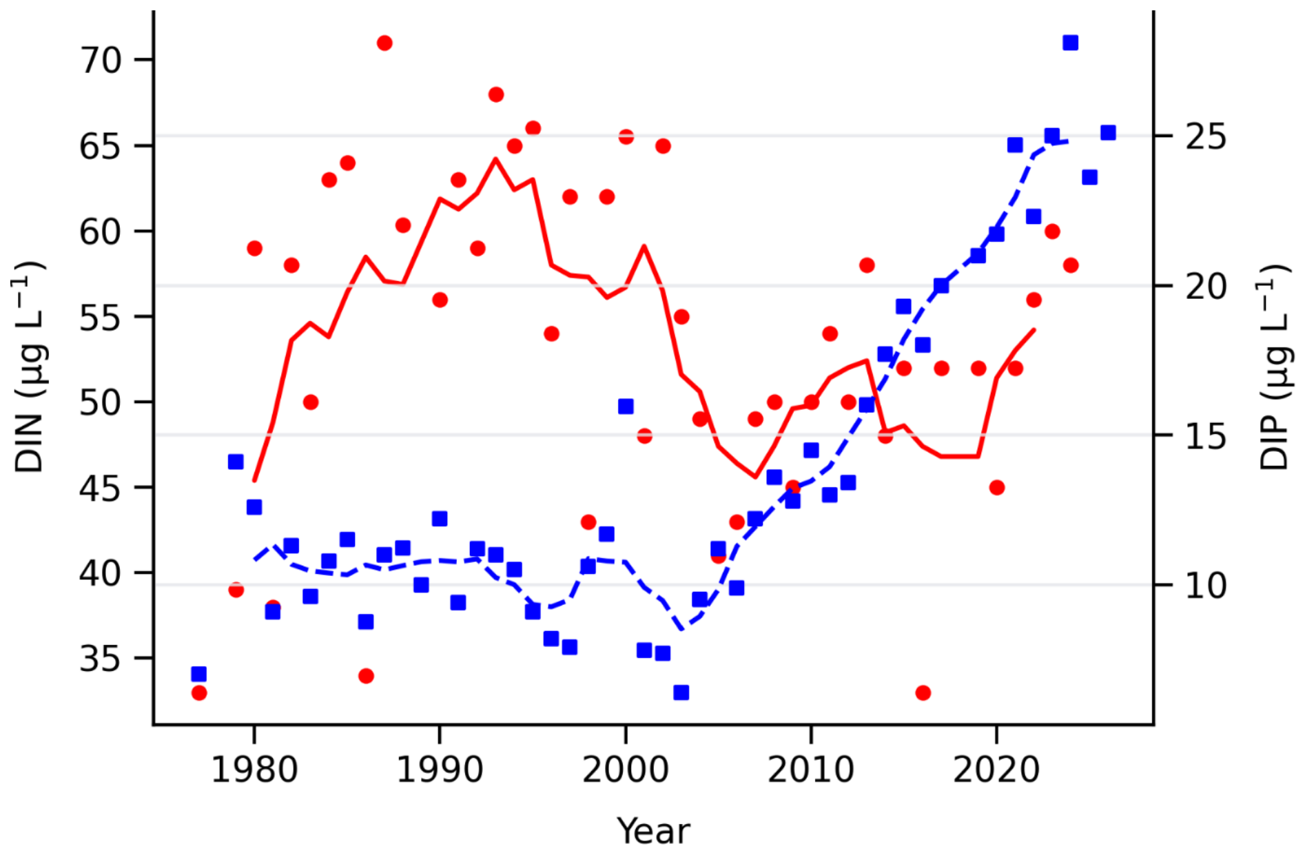
Wintertime concentrations of dissolved inorganic nitrogen (DIN) and dissolved inorganic phosphorus (DIP) exhibited contrasting long-term patterns at station SR5 (Figure 5). Annual mean DIP concentrations increased markedly over the study period, rising from approximately 7–12 µg L⁻¹ in the late 1970s–1980s to >20 µg L⁻¹ after 2010 (Figure 5).

In contrast, DIN concentrations showed no significant long-term trend (p > 0.05) and fluctuated primarily between ~40 and 65 µg L⁻¹ throughout the time series, with a near-zero Sen’s slope. The smoothed time series highlights a pronounced increase in DIP, particularly since the early 2000s, whereas DIN remained comparatively stable with moderate interannual variability.

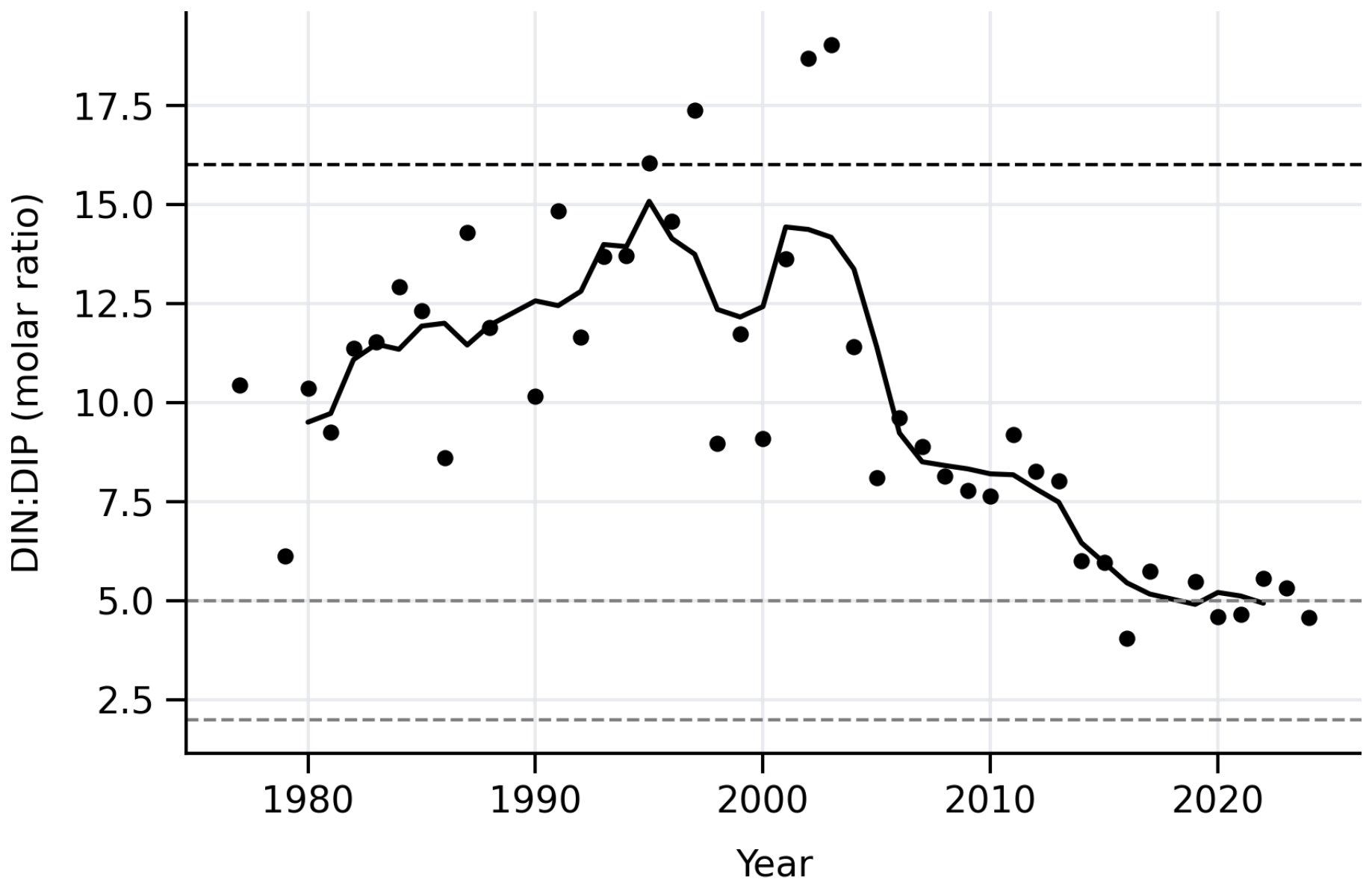
Consequently, the relative availability of nitrogen versus phosphorus has shifted over time, indicating a progressive decrease in the DIN:DIP molar ratio (Figure 6). The ratio declines from values around or above the Redfield ratio (16) in the early record to substantially lower levels in recent decades, with several years during the 2010s and 2020s showing values close to or below 5.

Overall, the DIN:DIP ratios spanned a wide range, from values indicative of phosphorus limitation (>16) in the earlier period to values associated with reduced phosphorus limitation and occasional nitrogen limitation (<5) in the later period. The smoothed trend demonstrates a persistent long-term decline, indicating an increasing relative importance of phosphorus in controlling nutrient balance.

3.3. Total Phosphorus and Dissolved Inorganic Phosphorus at Offshore Station SR5

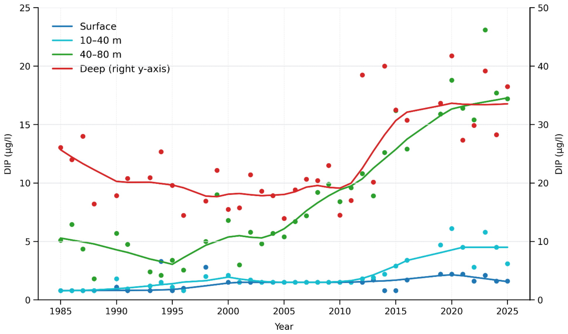
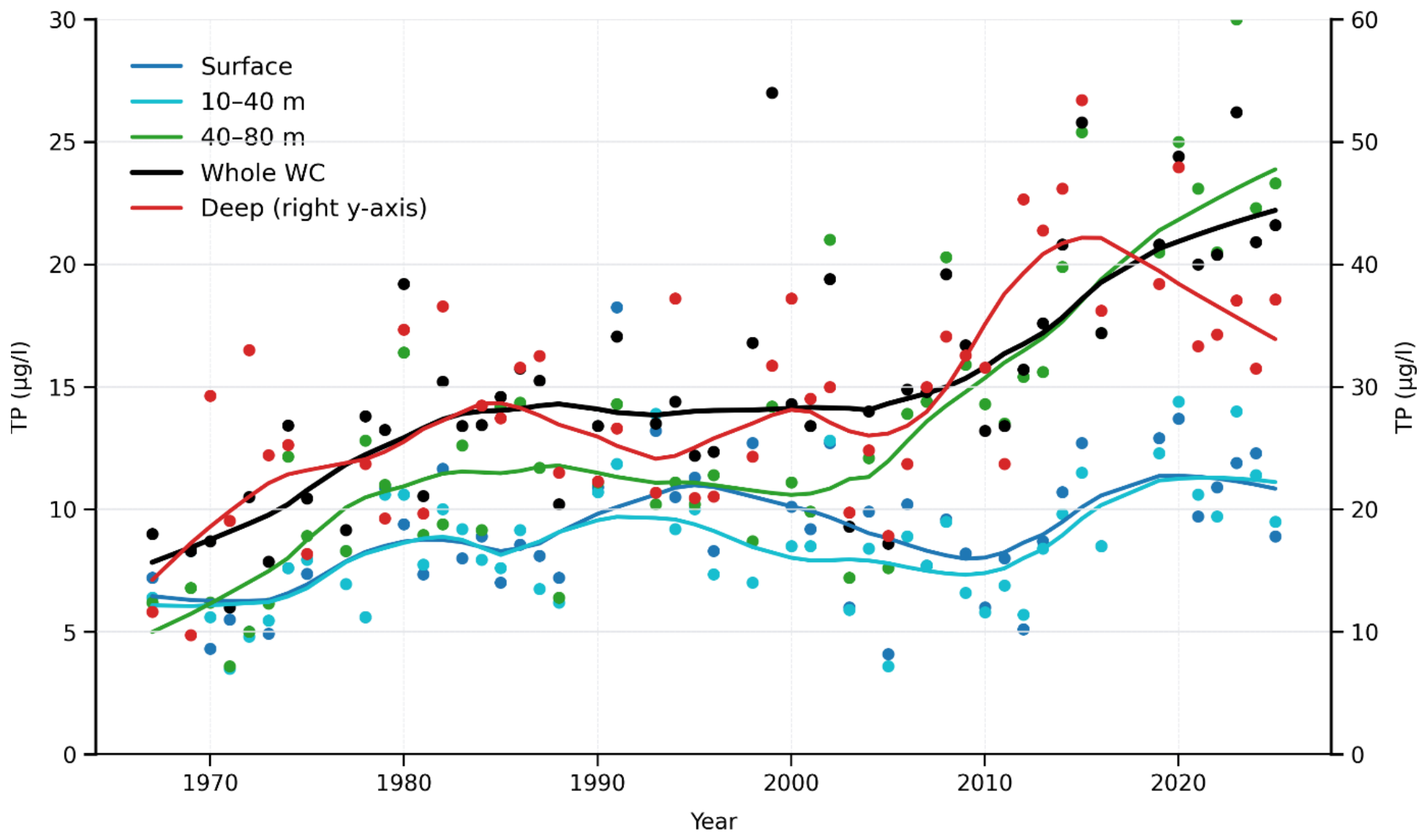
Summer TP and DIP concentrations at offshore monitoring station SR5 show pronounced long-term changes in both magnitude and vertical structure of the water column (Figure 7 and Figure 8). The development differs clearly between depth layers, with the strongest increases observed below the surface layer.

In the surface layer (0–10 m), TP concentrations remain relatively stable over the study period, and DIP concentrations are consistently low (<2–3 µg L⁻¹), with no robust long-term change evident in surface-layer phosphorus.

In the upper intermediate layer (10–40 m), both TP and DIP show clear increasing trends. DIP concentrations have risen from ~1–2 µg L⁻¹ to ~3–6 µg L⁻¹ since the mid-2000s, indicating a strengthening phosphorus signal below the surface layer.

The lower intermediate layer (40–80 m) exhibits a stronger increase in both TP and DIP, particularly after the early 2000s. DIP concentrations have risen from ~4–6 µg L⁻¹ to >15–20 µg L⁻¹ in recent years, and this layer shows pronounced enrichment and increasing variability.

The strongest changes occur in deep water (>80 m), where both TP and DIP increase markedly, with DIP rising from ~10–20 µg L⁻¹ to >30–40 µg L⁻¹. These results indicate substantial accumulation of bioavailable phosphorus in the deepest layer.

Whole water column TP also shows a clear long-term increase, with concentrations rising from ~13–16 µg L⁻¹ in earlier decades to >20 µg L⁻¹ after the mid-2000s (Figure 7).

Overall, both TP and DIP demonstrate a clear vertical decoupling in phosphorus dynamics. The absence of significant trends in the surface layer contrasts with strong and statistically robust increases below 10 m. The more pronounced increase in DIP relative to TP suggests that the long-term rise in phosphorus at SR5 is increasingly driven by the accumulation of dissolved, bioavailable phosphorus in intermediate and deep waters.

3.4. Spatial Variability and Temporal Trends in Chlorophyll a Across the Coastal–Offshore Gradient

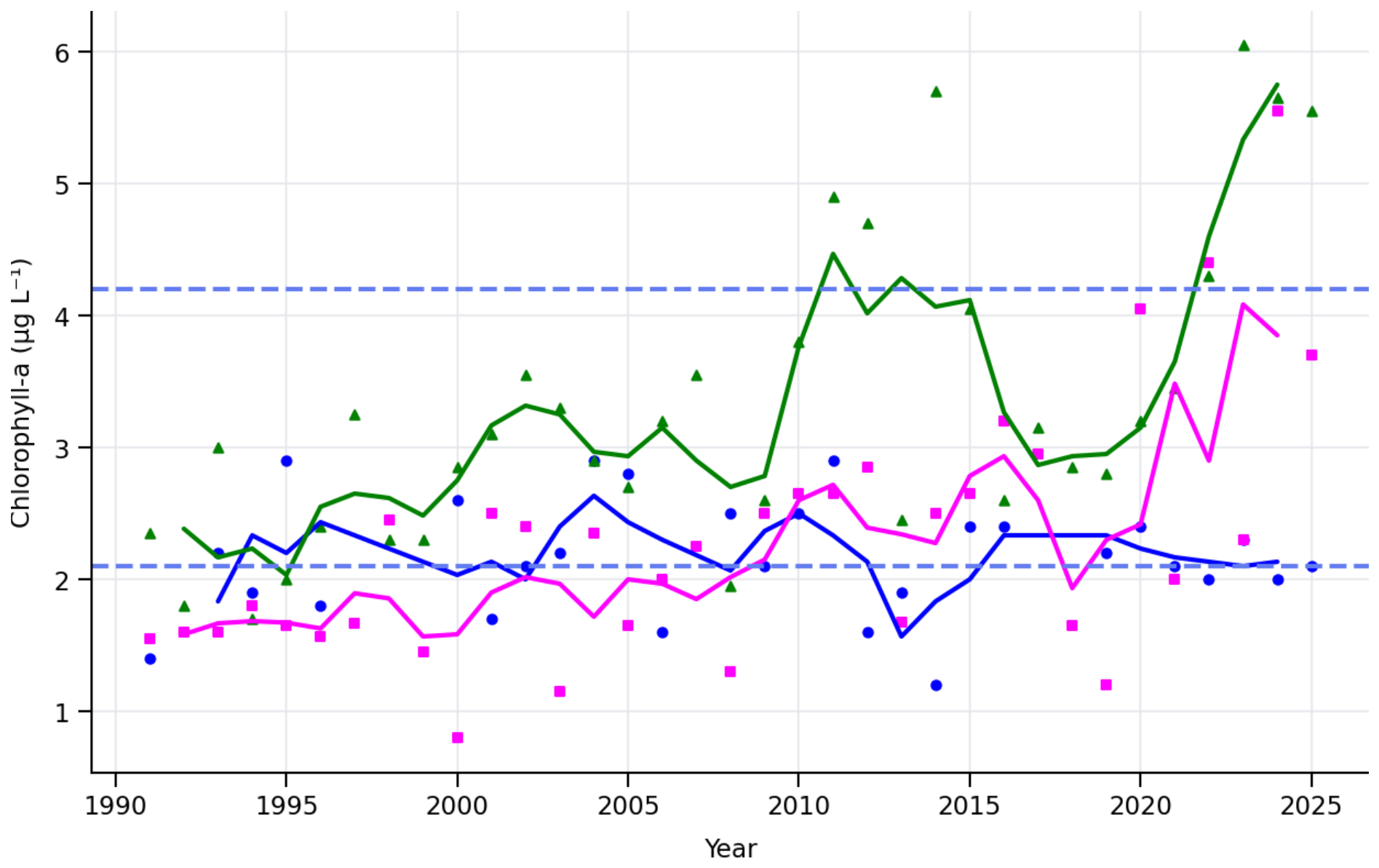
Chlorophyll-a concentrations exhibited clear spatial differences among the three monitoring stations over the period 1991–2025 (Figure 9). The offshore station SR5 showed low and relatively stable annual mean values, generally remaining close to the good ecological status boundary (2.1 µg L⁻¹) with only minor interannual variability.

At Rauma 435, chlorophyll a levels were higher and more variable than at SR5. Periods of elevated values were observed, particularly from the late 1990s onward. The smoothed time series suggests a gradual increase accompanied by pronounced interannual variability.

The inner archipelago station Uusikaupunki 105 consistently exhibited the highest chlorophyll a levels throughout the study period. The smoothed trajectory indicates a clear and statistically significant increasing trend since the early 2000s accompanied by substantial interannual variability.

Overall, the results reveal a strong gradient in chlorophyll-a concentrations, with lowest values at the offshore station, intermediate levels in the outer coastal zone, and highest concentrations in the inner archipelago.

3.5. Winter Total Nitrogen and Summer Chlorophyll a Along the Coastal Gradient off Uusikaupunki

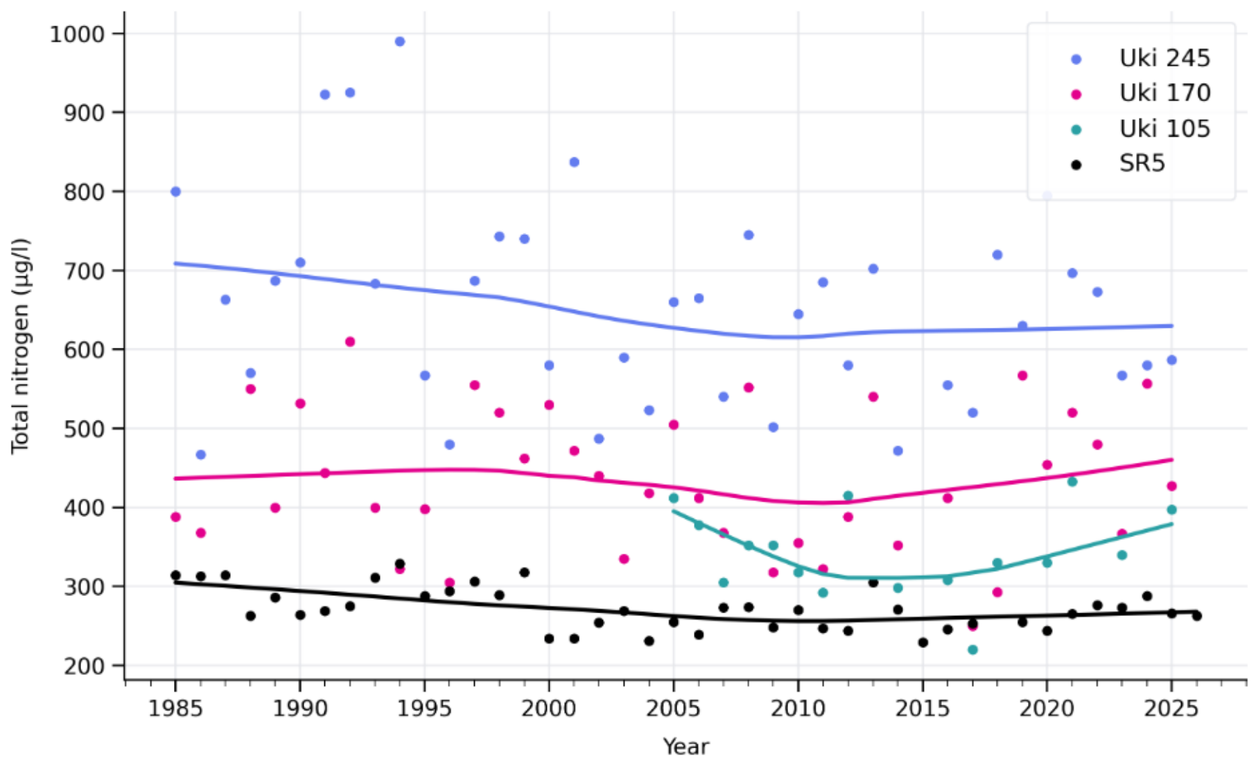
Winter total nitrogen (TN) concentrations integrated over the entire water column showed a clear coastal gradient among the monitoring stations (Figure 10). Mean TN concentrations were highest at Uki 245 (654.3 µg L⁻¹, n = 40) and decreased towards Uki 170 (433.0 µg L⁻¹, n = 39) and Uki 105 (337.9 µg L⁻¹, n = 15), with the lowest values observed at the offshore station SR5 (270.6 µg L⁻¹, n = 40). Median values followed the same pattern (Uki 245: 661.5 µg L⁻¹; Uki 170: 418.0 µg L⁻¹; Uki 105: 330.0 µg L⁻¹; SR5: 269.0 µg L⁻¹), confirming a consistent spatial gradient.

Variability was highest at the inner coastal station Uki 245 (467–990 µg L⁻¹; SD = 126.9) and decreased towards offshore waters, with intermediate variability at Uki 170 and Uki 105 and lowest variability at SR5.

Statistical analysis confirmed highly significant differences among stations (Kruskal–Wallis test, H(3) = 107.71, p < 0.001, ε² = 0.81), with all pairwise comparisons showing significant differences (Welch’s t-tests with Holm correction, all p < 0.001). These results demonstrate a strong and statistically robust decrease in winter TN concentrations from the inner coastal zone towards offshore waters.

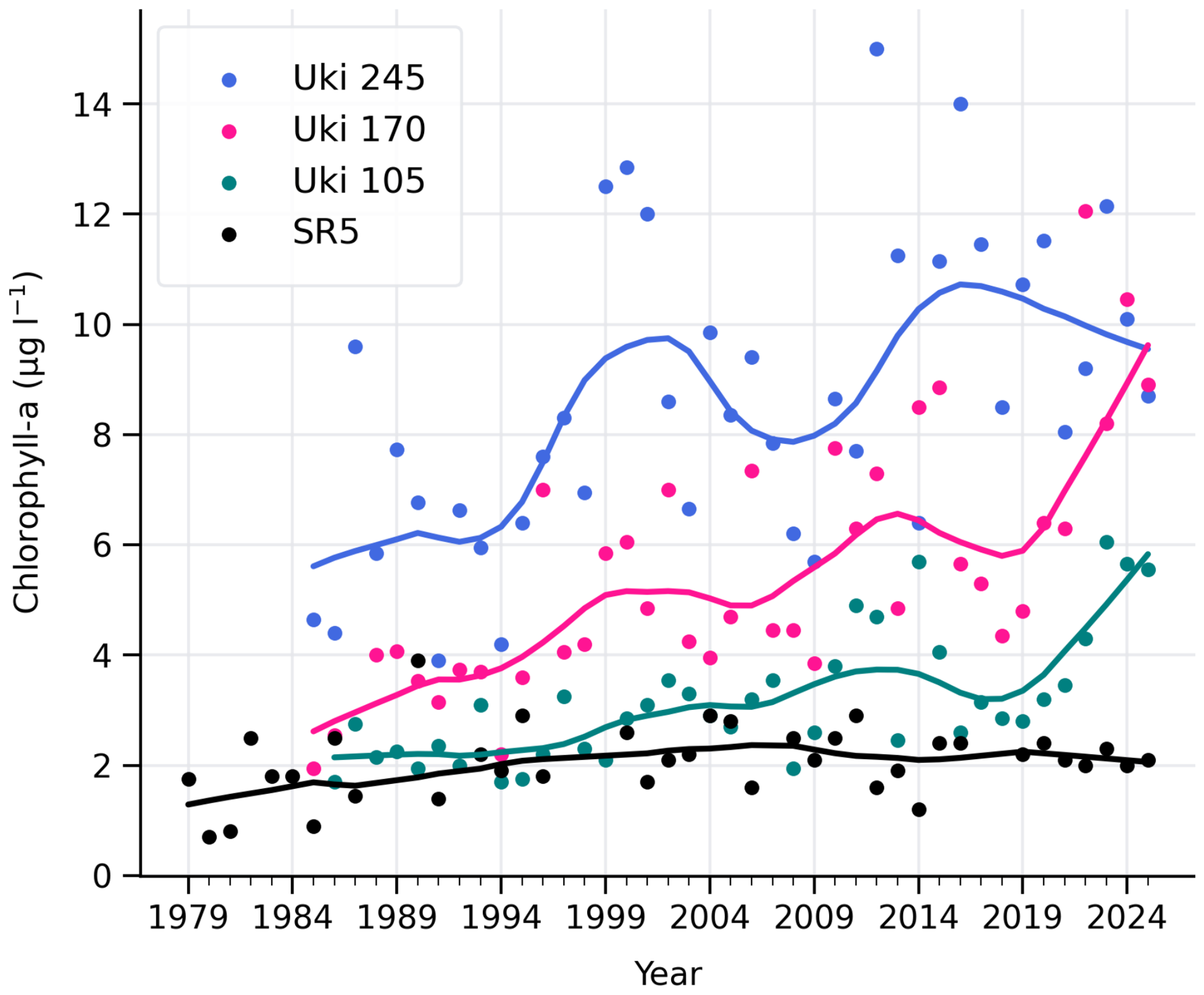
Summer chlorophyll-a concentrations showed a clear coastal–offshore gradient among the Uusikaupunki monitoring stations (Figure 11). Mean concentrations were highest at Uki 245 (8.6 µg L⁻¹, n = 41) and decreased towards Uki 170 (5.5 µg L⁻¹, n = 40) and Uki 105 (3.2 µg L⁻¹, n = 40), with the lowest values observed at the offshore station SR5 (2.1 µg L⁻¹, n = 38). Median values followed the same pattern, confirming a consistent offshore decrease in phytoplankton biomass.

Variability was highest at the inner coastal station Uki 245 (range 3.9–15.0 µg L⁻¹; SD = 2.73) and decreased towards offshore waters, with intermediate variability at Uki 170 and Uki 105 and lowest variability at SR5.

Statistical analysis confirmed highly significant differences among stations (Kruskal–Wallis test, H(3) = 112.6, p < 0.001), with all pairwise comparisons showing significant differences (Welch’s t-tests with Holm correction, all p < 0.001).

When evaluated against ecological status class boundaries, the observed gradient corresponds to a systematic decline in ecological status from inner coastal to offshore stations. Uki 245 falls within the moderate class and occasionally approaches the moderate–poor boundary, Uki 170 lies near the good–moderate boundary, and Uki 105 is generally within the moderate class, while SR5 remains within or close to the good class.

Before–after comparison indicates a clear temporal shift. Chlorophyll-a concentrations increased significantly after 2010 at Uki 170 (from 4.35 to 7.25 µg L⁻¹) and Uki 105 (from 2.55 to 4.08 µg L⁻¹), corresponding to a deterioration in ecological status. In contrast, no change was observed at the offshore station SR5.

Overall, the results demonstrate a strong coastal–offshore gradient in chlorophyll-a concentrations combined with a post-2010 deterioration in ecological status at intermediate and outer coastal stations, while offshore conditions remained comparatively stable.

3.6. Legacy Effects of Phosphogypsum-Derived Phosphorus Loading at Station UKI 170

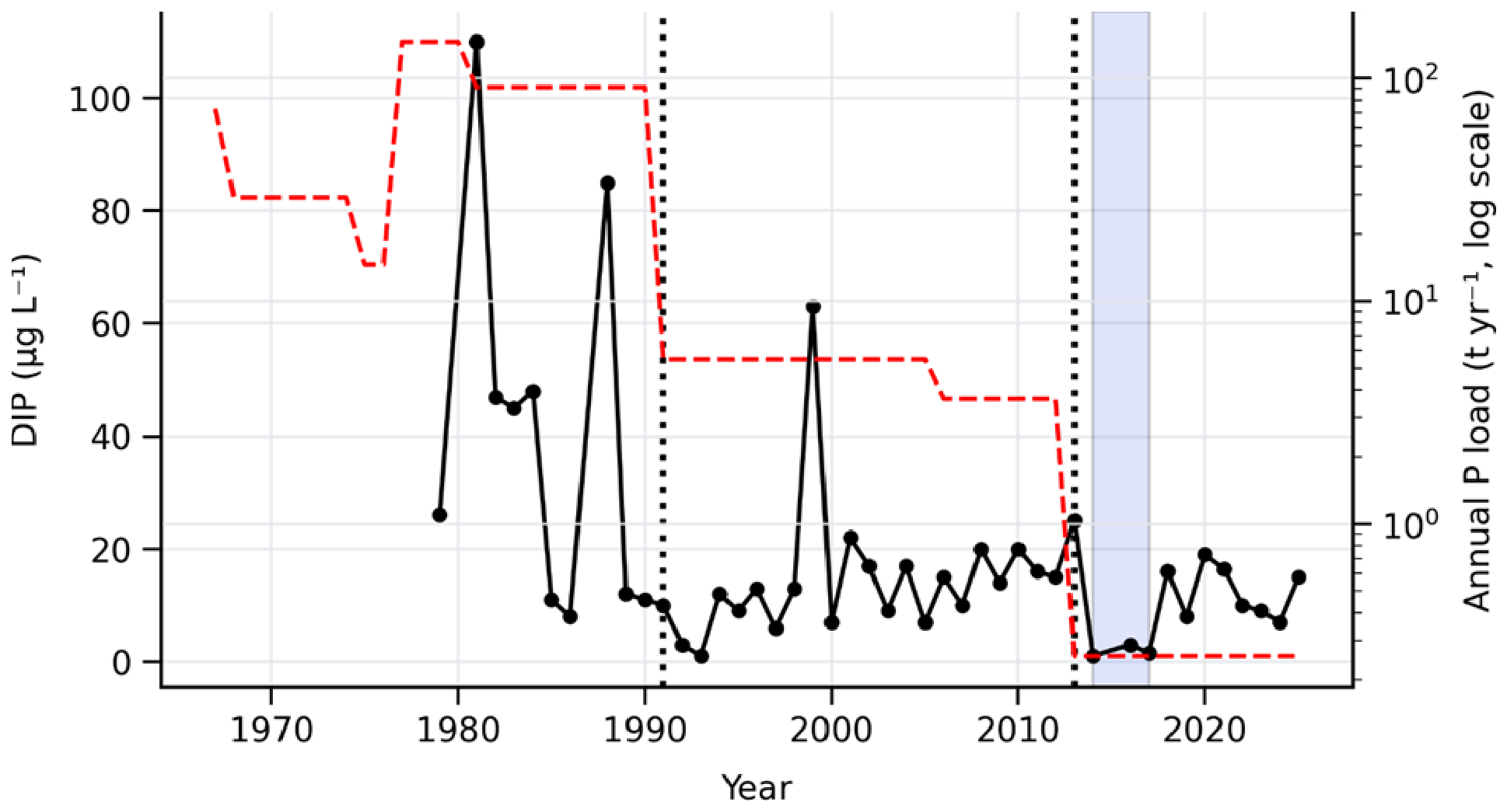
To evaluate the long-term impact of historical point-source loading, winter dissolved inorganic phosphorus (DIP) concentrations at station UKI 170 were compared with estimated phosphorus inputs from the Uusikaupunki phosphogypsum stack (see Section S1 in the Supplementary Materials; Figure 12).

The results show a clear temporal correspondence between high phosphorus loading and elevated DIP concentrations during the 1970s and 1980s, with values frequently exceeding 50–100 µg L⁻¹. Following the cessation of phosphoric acid production in 1991, DIP concentrations declined markedly, indicating a strong response to reduced external loading. However, concentrations did not immediately stabilize at low levels, and occasionally elevated values persisted into the late 1990s and 2000s, suggesting a delayed response due to internal storage and gradual release of previously accumulated phosphorus.

A further reduction in DIP concentrations after 2013 coincides with the installation of a cutoff wall and additional remediation measures. The period 2014–2017 is characterized by exceptionally low concentrations, often close to detection limits, indicating a strong but possibly temporary reduction in phosphorus leakage. After this period, DIP concentrations increased again to moderate levels (approximately 10–20 µg L⁻¹), suggesting partial recovery of background conditions or continued influence of residual phosphorus sources.

In contrast, summer chlorophyll-a concentrations at the same station do not show a direct one-to-one response to these changes (Figure 11). Elevated DIP concentrations during the early high-loading period were not associated with similarly high phytoplankton biomass, whereas the highest chlorophyll-a levels were observed during the later period after 2010, when winter DIP concentrations were already substantially lower. This indicates that the coupling between winter nutrient availability and summer phytoplankton biomass has changed over time.

Overall, the long-term development reflects a transition from extremely high phosphorus loading conditions to substantially lower but still elevated baseline levels. While the timing of major decreases in DIP concentrations is consistent with management interventions, the persistence of moderate concentrations—and the delayed and non-linear response of phytoplankton biomass—indicates that legacy effects and changing nutrient dynamics continue to influence the system.

3.7. Winter Total Nitrogen and Summer Chlorophyll a Along the Coastal Gradient off Rauma

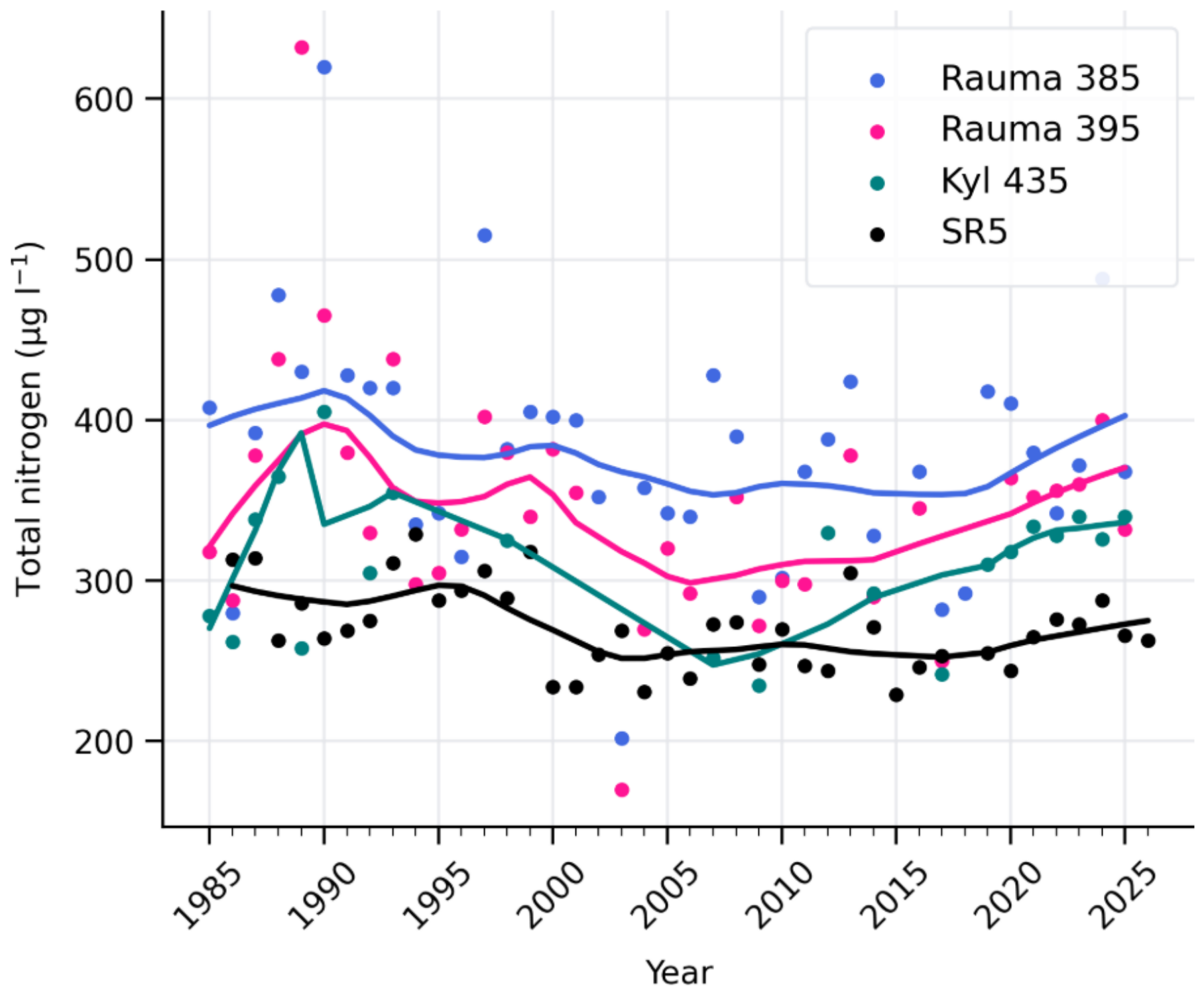
Winter total nitrogen (TN) concentrations integrated over the entire water column also showed a clear coastal–offshore gradient among the Rauma monitoring stations (Figure 13). Mean TN concentrations were highest at the inner coastal station Rauma 385 (380–390 µg L⁻¹, n = 40) and decreased towards Rauma 395 (330–350 µg L⁻¹, n = 35), with the lowest values observed at the outer station Kylmäpihlaja 435 (300–320 µg L⁻¹, n = 20). Median values followed the same pattern, confirming a consistent offshore decrease in winter TN concentrations.

Variability was highest at Rauma 385 (range 200–620 µg L⁻¹) and decreased towards offshore waters, with intermediate variability at Rauma 395 and lowest variability at Kylmäpihlaja 435.

Statistical analysis confirmed significant differences among stations (Kruskal–Wallis test, H(2) ≈ 22, p < 0.001, ε² ≈ 0.25). Pairwise comparisons showed that Rauma 385 differed significantly from both Rauma 395 and Kylmäpihlaja 435, while the difference between Rauma 395 and Kylmäpihlaja 435 was weaker but remained significant.

To assess temporal changes, coastal–offshore differences relative to SR5 were analysed (ΔTN = TN_station − TN_SR5). The average gradient increased from approximately 60–90 µg L⁻¹ before 2010 to 90–120 µg L⁻¹ after 2010, indicating a statistically significant strengthening of the coastal–offshore gradient over time.

Overall, the results demonstrate a clear spatial gradient in winter TN concentrations, together with a temporal intensification of the coastal signal in the Rauma area.

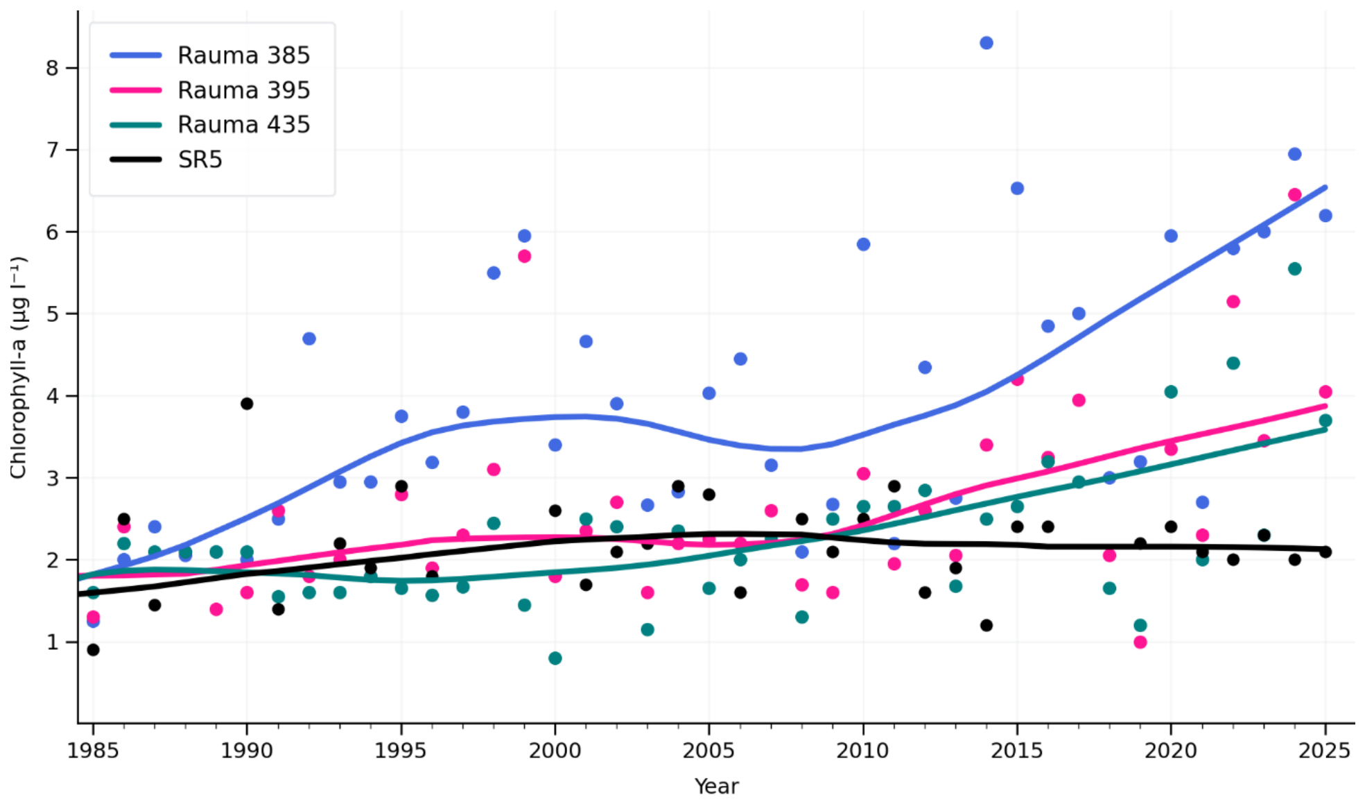
To examine temporal changes in chlorophyll-a concentrations, the dataset was divided into two periods (1985–2009 and 2010–2025), based on a basin-scale shift in phosphorus dynamics observed at the offshore station SR5 (Figure 8). Dissolved inorganic phosphorus (DIP) concentrations increased markedly in intermediate layers after approximately 2010, indicating enhanced accumulation of bioavailable phosphorus in the water column, while no corresponding increase was observed in surface waters.

At the same time, phosphorus loading in the Rauma coastal area showed a contrasting development. Inputs increased substantially from the late 1990s to a peak during 2005–2009 but thereafter decreased markedly. Thus, the post-2010 period is characterized by decreasing local phosphorus loading but increasing basin-scale phosphorus availability.

Despite the reduction in local phosphorus inputs, chlorophyll-a concentrations increased significantly at all coastal stations during the later period (Figure 14), while no change was observed at the offshore reference station SR5.

When evaluated against ecological status class boundaries, this increase corresponds to a systematic shift towards lower status classes at the coastal stations. Rauma 395 and Rauma 435 shifted from good or near-good conditions before 2010 to clearly moderate conditions thereafter, while Rauma 385 increased from moderate levels towards the moderate–poor boundary.

This shift is also evident in the distribution of observations among ecological status classes. At Rauma 435 and Rauma 395, good status dominated before 2010, whereas moderate status clearly prevailed after 2010. At Rauma 385, the distribution shifted towards a predominance of moderate conditions and frequent values close to the moderate–poor boundary, while SR5 remained largely within the good class throughout the monitoring period.

Prior to 2010, chlorophyll-a concentrations at Rauma 395 and Rauma 435 were relatively close to offshore values, indicating a weak coastal–offshore gradient. After 2010, both stations exhibited consistently higher concentrations than SR5, reflecting a clear strengthening of the coastal signal, while Rauma 385 maintained the highest levels throughout the period.

Overall, the results indicate a dual control of eutrophication dynamics in the Rauma coastal zone: basin-scale phosphorus enrichment drives the long-term increase in phytoplankton biomass, while local gradients and nearshore processes maintain a strong and persistent coastal–offshore structure.

3.8. Long-Term Increase and Variability in Nostocales Biomass at SR5 and Kylmäpihl 435, and Comparison with UKI 105

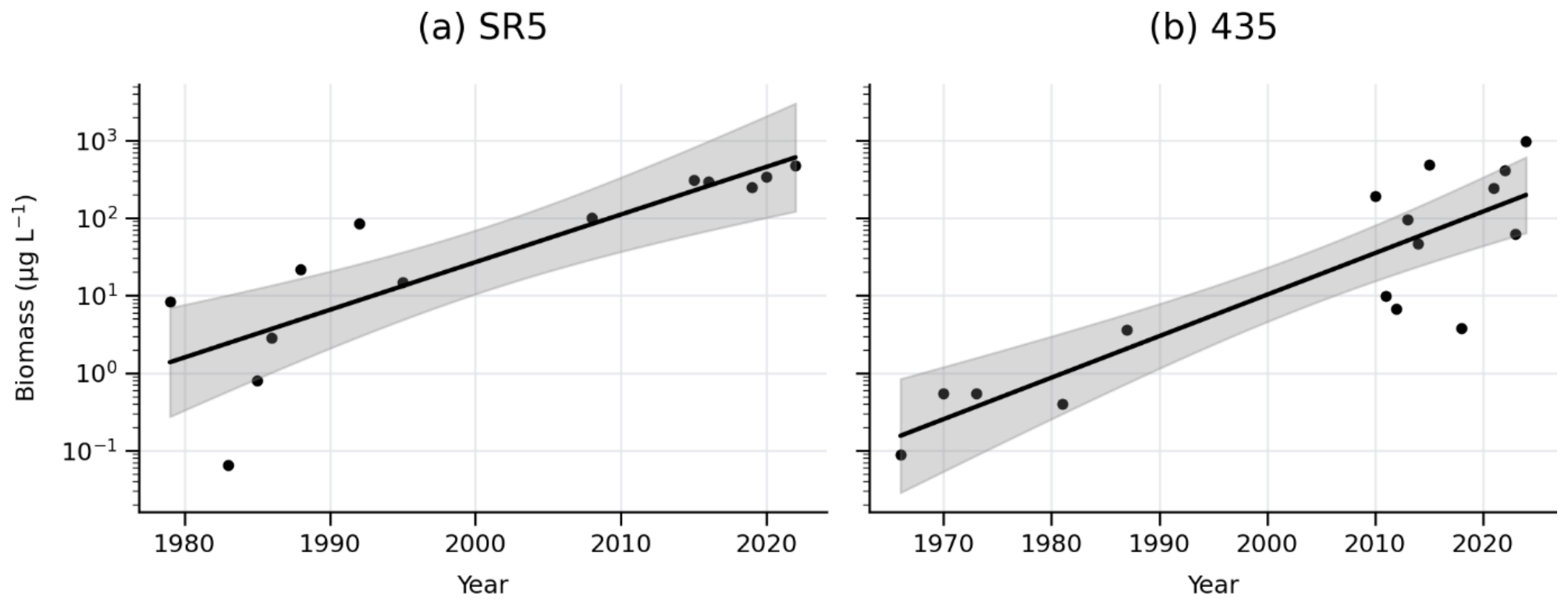
The time series of nitrogen-fixing cyanobacteria (order Nostocales) at coastal stations SR5 and Kylmäpihl 435 (Bothnian Sea) shows a pronounced long-term increase in summer biomass (Figure 15). During the first decades of monitoring (1960s–1980s), biomass at station 435 remained consistently low, typically below 1–5 µg L⁻¹, with only occasional minor peaks, while SR5 exhibited similarly low levels with somewhat higher interannual variability. From the early 2000s onwards, Nostocales biomass increased markedly at both stations, accompanied by a clear intensification in the frequency and magnitude of bloom events. At station 435, biomass values exceeding 300 µg L⁻¹ became common during peak years, with extreme values surpassing 1000 µg L⁻¹ recorded in recent decades, whereas SR5 shows a comparable increase.

Temporal development is characterized not by a gradual increase but by strong interannual variability, with distinct blooming years alternating with years of relatively low biomass, indicating episodic dynamics superimposed on a long-term upward trend. Linear regression fitted to log₁₀-transformed annual biomass confirms a statistically highly significant increase over time at both stations (station 435: β ≈ 0.060 yr⁻¹, p < 0.001, R² ≈ 0.56; SR5: β ≈ 0.061 yr⁻¹, p < 0.001, R² ≈ 0.71), corresponding to approximately exponential growth and an average annual increase of about 15% at both locations.

Recent observations from station UKI 105 (Iso-Hylkimys, Uusikaupunki), covering the period 2017–2025, indicate consistently high Nostocales biomass characteristic of present-day conditions. Biomass is strongly dominated by Aphanizomenon, with annual peak values typically ranging from approximately 40 to over 500 µg L⁻¹ and occasionally exceeding 1000 µg L⁻¹ in extreme years. Dolichospermum contributes variably, generally within the range of ~3–100 µg L⁻¹, while Nodularia spumigena occurs episodically with lower but sometimes notable biomass. Overall, mean summertime biomass at UKI 105 is on the order of several hundred µg L⁻¹ for Aphanizomenon-dominated blooms, placing current conditions clearly within the high-biomass state observed during the most recent decades at SR5 and station 435.

Changes in taxonomic composition further indicate that the observed increase is primarily driven by Aphanizomenon, which dominates most bloom events across all stations, whereas Dolichospermum and Nodularia contribute episodically and exhibit substantial interannual variation. In earlier decades, Anabaena was relatively more common but has declined in relative importance. The increasing Nostocales biomass coincides with periods of elevated phosphorus availability and increasing chlorophyll a concentrations in the coastal zone, suggesting a broader shift in ecosystem functioning toward conditions favoring cyanobacterial blooms. Overall, these results indicate a transition from a historically low-biomass system to one increasingly characterized by episodic high-biomass bloom events, with present-day conditions, as represented by UKI 105, firmly reflecting this intensified state of nitrogen-fixing cyanobacteria in the outer coastal zone of the Bothnian Sea.

4. Discussion

The results indicate that eutrophication in the Bothnian Sea coastal zone is increasingly controlled by basin-scale phosphorus enrichment originating from the Baltic Proper, superimposed on locally driven nutrient inputs and internal biogeochemical feedbacks. The observed increase in phosphorus transport and its accumulation within the water column indicates a long-term expansion of the effective phosphorus reservoir, consistent with large-scale changes in Baltic Sea nutrient dynamics and internal loading processes [3,5,9]. This interpretation is supported by studies highlighting the dominant role of internal phosphorus sources in sustaining elevated nutrient levels in the Baltic Proper [6,7].

The vertical structure observed at station SR5, where total phosphorus (TP) and dissolved inorganic phosphorus (DIP) increase below the surface layer while remaining stable at the surface highlights the importance of subsurface accumulation and vertical redistribution. Intermediate and deep layers thus function as key storage compartments that prolong phosphorus residence time and enhance internal cycling, a mechanism widely documented in stratified Baltic Sea systems [5,9]. The concept of a large offshore nutrient reservoir is also consistent with assessments of the Baltic Sea winter nutrient pool distribution [34].

This development is consistent with intensified internal phosphorus loading in the Baltic Proper, where hypoxia has increased sediment–water phosphorus fluxes and elevated deep-water DIP concentrations [7,9]. Several studies have shown that internally sustained phosphorus inputs can dominate over reductions in external loading and maintain eutrophic conditions over long timescales [6,7,11].

Subsequent northward transport of phosphorus-rich waters contributes to increasing phosphorus availability in the Bothnian Sea and promotes a shift toward nitrogen limitation [5]. At the same time, the absence of hypoxia at SR5, a pelagic offshore station in the Bothnian Sea, indicates that local sediment release is not the dominant mechanism, and that the observed patterns are primarily driven by large-scale transport combined with vertical redistribution within the water column.

A key ecological consequence of this development is the decline in winter DIN:DIP ratios, indicating a shift toward nitrogen limitation. Such stoichiometric shifts are known to fundamentally alter phytoplankton competition by favoring diazotrophic cyanobacteria capable of utilizing atmospheric nitrogen [3,46]. Experimental and observational studies have demonstrated that nutrient limitation patterns in the Baltic Sea are strongly governed by spatial gradients in stoichiometry and eutrophication intensity [13]. This mechanistic interpretation is strongly supported by recent large-scale synthesis results from the Bothnian Sea, which show a consistent long-term shift toward nitrogen limitation driven by rising phosphorus concentrations and declining DIN:DIP ratios [47].

In parallel, increases in primary production and phytoplankton biomass observed across multiple monitoring stations indicate a basin-wide intensification of biological activity consistent with eutrophication processes [47]. Recent ecosystem-scale analyses further demonstrate that such changes are reflected at higher trophic levels, indicating broader food-web impacts of eutrophication in the Bothnian Sea [48].

This mechanism provides an explanation for the observed long-term increase in nitrogen-fixing cyanobacteria (Nostocales) in the coastal zone, linking basin-scale phosphorus enrichment to biological community change. Rather than representing a gradual linear response, the development is characterized by episodic but increasingly frequent high-biomass bloom events, indicating that long-term nutrient enrichment interacts with interannual variability in physical conditions. Physical drivers such as upwelling events have been shown to trigger cyanobacterial blooms under favorable conditions, further contributing to temporal variability [49]. The persistence of high Nostocales biomass in recent observations, including UKI 105, further indicates a transition toward consistently elevated cyanobacterial biomass, reflecting sustained changes in nutrient conditions and ecosystem functioning rather than a formally defined regime shift.

The increasing dominance of filamentous cyanobacteria, particularly Aphanizomenon, observed in this study is consistent with regional assessments indicating that cyanobacterial biomass is associated with nitrogen limitation and low DIN:DIP ratios [47]. Monitoring synthesis studies further highlight the importance of methodological and environmental variability in detecting cyanobacterial dynamics across the Baltic Sea [50]. Importantly, these large-scale analyses also indicate substantial spatial heterogeneity and interannual variability in cyanobacterial occurrence, supporting the interpretation that the observed increase represents a recurring pattern rather than a uniform intensification across all areas [47].

The increasing dominance of Aphanizomenon under these conditions likely reflects not only low DIN:DIP ratios and nitrogen limitation but also taxon-specific ecophysiological traits. Unlike some strictly diazotrophic cyanobacteria, Aphanizomenon can utilize combined nitrogen when available and exhibits considerable ecological flexibility. Its ability to regulate buoyancy and exploit stratified conditions enables efficient access to phosphorus-rich layers, while adaptation to low-light and variable nutrient environments supports persistence in the northern Baltic Sea. Consequently, its dominance is best understood as the result of interacting controls, where nutrient stoichiometry creates favorable conditions for diazotrophs in general, but species-specific functional traits determine competitive success [3,13,50].

Despite the dominant role of basin-scale phosphorus enrichment, the results clearly demonstrate that local nutrient loading remains a critical controlling factor in coastal areas. Strong and persistent coastal–offshore gradients in winter total nitrogen and summer chlorophyll a in both the Uusikaupunki and Rauma regions indicate that local inputs significantly elevate nutrient concentrations and biological production in nearshore waters. The consistency of these gradients, together with systematically poorer ecological status toward inner coastal stations, demonstrates that local loading continues to control the spatial structure of eutrophication.

The importance of local processes is particularly evident in the Uusikaupunki area, where legacy effects from historical phosphorus loading have resulted in prolonged elevation of dissolved phosphorus concentrations despite substantial reductions in external inputs. The delayed response reflects long-term storage and gradual release of phosphorus previously accumulated in sediments and the water column, highlighting that past point sources can exert multi-decadal impacts and continue to influence ecosystem functioning. Such long-term persistence of internal nutrient sources counteracting external load reductions has been widely documented in Baltic coastal systems [11].

A similar interaction between local and basin-scale drivers is observed in the Rauma coastal zone. Although local phosphorus inputs have decreased since the late 2000s, phytoplankton biomass has increased, indicating that basin-scale phosphorus enrichment elevates background nutrient availability and sustains biological production. At the same time, the ecological response is strongly modulated by hydrodynamic conditions. In relatively open coastal systems such as Rauma, short water residence times and efficient water exchange limit nutrient retention and reduce the direct influence of local inputs. Consequently, basin-scale forcing primarily determines the baseline trophic state, while local nutrient inputs and water residence time regulate the magnitude and spatial variability of phytoplankton biomass, particularly along the coastal–offshore gradient. This explains why phytoplankton biomass has increased despite reduced local phosphorus loading, while persistent coastal gradients continue to reflect the influence of local processes.

These observations demonstrate a dual-control system in which basin-scale phosphorus enrichment determines the long-term trophic trajectory, while local nutrient loading and legacy effects control spatial variability in ecological status. Together, the results show that eutrophication dynamics in the Bothnian Sea coastal zone emerge from interactions across multiple spatial scales, with large-scale nutrient enrichment establishing the regional background state and local processes determining its ecological expression. More broadly, these findings indicate that similar cross-scale interactions between external nutrient inputs, internal feedback mechanisms, and basin-scale physical forcing are fundamental features of eutrophication in inland and semi-enclosed marine systems. As these interactions can generate non-linear ecosystem responses and delay recovery even following reductions in external loading, effective management requires coordinated measures addressing both regional nutrient transport and local sources.

5. Conclusions

Eutrophication in the coastal Bothnian Sea is driven by interacting processes operating across multiple spatial scales. Basin-scale phosphorus enrichment originating from the Baltic Proper increasingly determines background conditions, whereas local nutrient inputs regulate coastal responses. The accumulation of phosphorus in intermediate and deep waters, sustained by internal loading and northward transport, has expanded the offshore phosphorus reservoir and enhanced internal phosphorus cycling [3,5,9]. This is consistent with the dominant role of internal phosphorus sources in sustaining eutrophication in the Baltic Proper [6,7].

Declining DIN:DIP ratios indicate a shift toward nitrogen limitation [44]. Under these conditions, phosphorus availability increasingly controls nitrogen fixation and, consequently, phytoplankton production [13]. These changes are reflected in the observed increase in nitrogen-fixing cyanobacteria and overall phytoplankton biomass, indicating a transition toward a phosphorus-driven ecosystem state with effects extending to higher trophic levels [48].

Despite strong basin-scale forcing, persistent coastal–offshore gradients indicate that local nutrient inputs remain a key driver of spatial variability and ecological status. Legacy effects further delay recovery by sustaining elevated nutrient concentrations despite reductions in external loading [11].

Overall, eutrophication is governed by a dual-control system in which basin-scale processes determine long-term trophic conditions, whereas local nutrient inputs regulate their spatial expression. From a management perspective, local measures remain essential but should be complemented by coordinated basin-scale actions. Recovery is therefore likely to remain slow under persistently elevated background phosphorus conditions [6,7].