Robust Features, Adaptive Thresholds: LightGBM for Fishing Vessel Type Identification from Sparse AIS Data

Abstract

Under 10 min sparse Automatic Identification System (AIS) sampling, the reliability of point-wise motion statistics degrades substantially, and conventional classification methods rely on trajectory interpolation, which may introduce spurious motion patterns. This study proposes a feature-driven framework for fishing vessel type identification that eliminates the need for interpolation preprocessing. A 39-dimensional feature set is constructed using robust statistics, including the median and interquartile range, to characterize trajectory-level behavioral patterns. Adaptive speed interval thresholds are derived through a data-driven approach grounded in Bayesian decision boundaries, thereby removing the dependence on manually defined cut-off values. A backward ablation procedure guided by feature importance ranking identifies a lightweight 12-dimensional feature subset that retains 98.7% of the classification accuracy at a compression rate of 69%. Evaluated on 18,320 fishing vessel trajectories in the East China Sea, the full 39-dimensional feature set achieves a 5-fold cross-validation accuracy of 91.92% (Macro-F1 = 0.919, Kappa = 0.879), with inter-fold standard deviations ranging from 0.002 to 0.004. Comparative experiments demonstrate that three tree-based classifiers all exceed 90% accuracy on the same feature set, confirming that feature robustness, rather than model selection, constitutes the dominant performance factor. LightGBM achieves the optimal trade-off between accuracy and training efficiency, whereas the cross-validation standard deviation of LSTM is approximately 7.5 times greater, indicating that hand-crafted robust features provide superior stability under sparse sampling conditions. The proposed framework requires no fishery-specific prior knowledge and offers a transferable paradigm for sparse AIS trajectory analysis.

1. Introduction

Marine fisheries are a vital pillar of global food security, but their sustainability faces dual threats from overexploitation and illegal, unreported and unregulated (IUU) fishing. The FAO (2024) assessment shows [1] that approximately 37.7% of global fishery resources are already overfished. Accurately identifying the operational type of fishing vessels is not only a prerequisite for formulating differentiated fisheries management policies, but also an effective method for detecting the inconsistency between registered vessel types and actual operational behavior.

AIS trajectory data-driven vessel behavior analysis has been an active research area in recent years. Yang et al. [2] provide a comprehensive review of machine learning applications in AIS data-driven maritime research, while Cheng et al. [3] focus on reviewing the progress of artificial intelligence methods in fishing vessel behavior recognition. Existing fishing vessel type identification methods can be categorized into four groups, namely, methods based on handcrafted statistical features and machine learning, methods based on trajectory imaging and deep learning, methods based on sequence modeling and deep learning, and methods based on multimodal fusion. In the category of handcrafted features, Guan et al. [4] extract 72-dimensional speed and course statistical features and achieve 95.68% accuracy using LightGBM for classifying trawlers, gillnetters, and purse seiners. Wang et al. [5] propose a multi-feature engineering framework that, with the assistance of large language model optimization, achieves 94.1% accuracy by combining 28-dimensional features with LightGBM. Cheng et al. [6] construct a 58-dimensional vector by fusing geometric and dynamic features, filter it with XGBoost, and then employ a BiLSTM-CNN-Attention model to reach 91.90% accuracy. For sequence modeling approaches, Kong et al. [7] propose SeaTraNet, a dual-path model for single trawler anomalous behavior detection, and Shin et al. [8] propose an HMM-DNN-CNN fusion model that achieves an F1 score of 97.54% based on trajectory features for four vessel types including fishing vessels. In trajectory imaging, Chen et al. [9] encode AIS trajectories into images for CNN-based vessel motion pattern classification. Zhao et al. [10] present CNN-Lite, a lightweight model that maps trajectory dynamic features into RGB three-channel images for vessel motion state recognition. Shahir et al. [11] propose the GIST method, which converts trajectory segments into two-dimensional histogram images and reaches 97% accuracy with a 3D-CNN. Hu et al. [12] employ Gramian angular field encoding to transform AIS sub-trajectory time series into multi-channel image representations and combine it with a hierarchical Transformer for fishing vessel behavior pattern recognition. In multimodal fusion, Du et al. [13] propose MM-FishingNet, which fuses time-frequency features and trajectory images to classify trawlers, purse seiners, and gillnetters with an accuracy of 92.23%. Additionally, Yu et al. [14] adopt a dilated CNN-IndRNN architecture to classify fishing vessel operational types with 93.12% accuracy.

Despite the positive progress made in the above studies, several issues remain insufficiently addressed. Existing feature engineering is largely designed for high-frequency AIS data, and under a 10 min sparse sampling interval the statistical reliability of point-wise motion variations decreases, causing the original features to adapt poorly to new datasets. Speed interval segmentation often relies on manually defined thresholds and lacks data-driven adaptivity. Moreover, current AIS trajectory analysis pipelines commonly treat interpolation as a necessary preprocessing step, since deep sequence models require uniformly spaced inputs and thus rely on interpolation and resampling to regularize irregular AIS time series [15].

These issues are closely intertwined under sparse sampling conditions. At 10 min intervals, behavioral signals in raw coordinate sequences are substantially attenuated, which limits the effectiveness of end-to-end deep models in extracting discriminative temporal patterns. Under such conditions, a feature-driven approach that replaces point-wise variations with robust statistical aggregation can better preserve behavioral signals, while data-driven adaptive thresholds remove the need for manual specification. By encoding domain knowledge into the feature design, such a framework may also reduce the dependence on large-scale labeled datasets that end-to-end models typically require. Accordingly, this study proposes a feature-driven classification framework tailored for sparse AIS data and validates its effectiveness and model independence through systematic comparison across multiple classifier architectures.

This paper makes three primary contributions. First, it proposes a sparse data processing paradigm that directly extracts features from sparse trajectories, replaces point-wise precise variations with robust statistics, and constructs a 39-dimensional sparse robust feature set; comparative experiments further verify the classification advantage of this feature set for different models operating on sparse data. Second, it employs a Gaussian Mixture Model to automatically learn the underlying speed distribution structure and adaptively determines speed interval boundaries as a preliminary step for feature extraction, requiring no manual intervention. Third, ablation experiments reveal the marginal decay pattern of accuracy with increasing feature dimensionality, and a 12-dimensional lightweight feature subset retains 98.7% accuracy at a compression rate of 69%, offering a reference for feature-driven lightweight deployment.

2. Materials and Methods

2.1. Data Preprocessing

The dataset used in this study is publicly available from the HeyWhale open data platform (https://www.heywhale.com/mw/dataset/623b00c9ae5cf10017b18cc6/content, accessed on 6 February 2026). This open-source AIS dataset comprises real historical vessel trajectory data collected from Chinese offshore waters, with the original data derived from vessel traffic in the East China Sea.

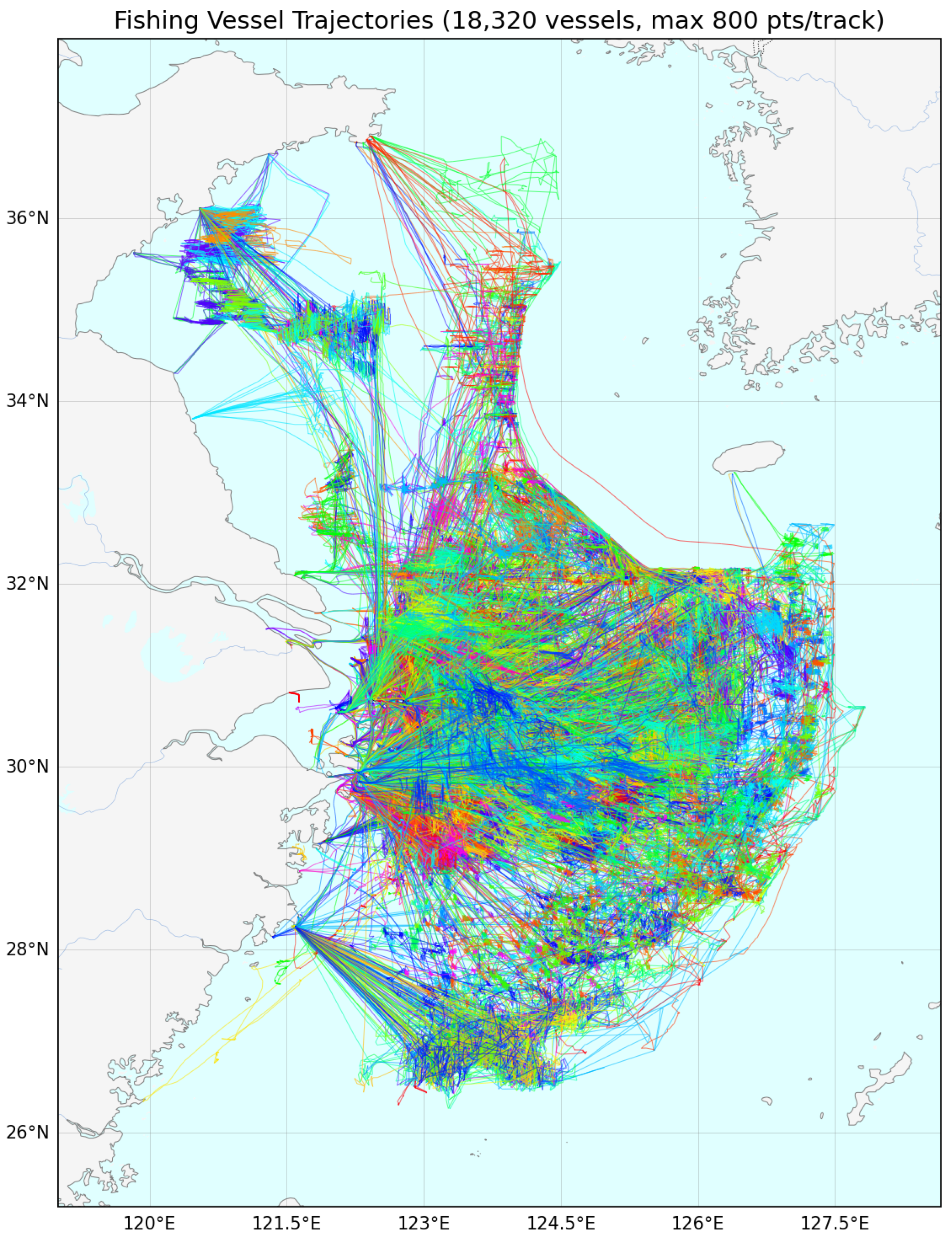
The AIS data used in this study cover fishing vessel trajectory records in the East China Sea (21° N to 37° N, 115° E to 130° E), spanning from September 2016 to November 2020. The dataset comprises 18,320 CSV files, each corresponding to one or more trips of a single fishing vessel, and covers three operational types registered by the fisheries authority: trawler, gillnetter, and purse seiner. The AIS data have been de-identified, and the original fields include vessel ID, timestamp (time), longitude, latitude, speed (Speed), course over ground (Type), and vessel type. The data are predominantly sampled at a 10 min interval, and irregular sampling also occurs. Given the large number of trajectory points, the trajectories are downsampled to produce an overview map, as shown in Figure 1.

Prior to the experiments, trajectory data cleaning is required. Zhang and Zhou [16] proposed a fishing vessel trajectory outlier detection method based on the Geohash geocoding algorithm, providing a reference for broadening the approaches to data cleaning. This paper implements the following cleaning rules:

Missing value handling: records with empty values in any of the fields of timestamp, longitude, latitude, speed, or course are removed.

Duplicate record removal: for duplicate trajectory points with identical timestamps, only the first record is retained; for records with different timestamps but identical longitude, latitude, speed, and course while the speed is non-zero, the subsequent duplicates are deleted.

Speed anomaly filtering: since the maximum speed of a fishing vessel generally does not exceed 20 knots, records with speed greater than 30 knots or less than 0 knots are treated as anomalies and removed.

Course anomaly filtering: the valid range of the course field is 0° to 360°, and records outside this range are deleted.

Abnormal drift detection: for adjacent trajectory points, the spherical distance is calculated using the Haversine formula. If this distance exceeds the theoretical distance that a fishing vessel can travel at maximum speed within the same time interval, the latter point is identified as an abnormal drift point and removed. The detection rule is:

$$d(p_i,p_{i+1})>v_{max}\times (t_{i+1}-t_i)$$

(1)

where $d(p_i,p_{i+1})$ is the spherical distance between two adjacent points, $v_{max}$ denotes the maximum speed of the fishing vessel, and $t_{i+1}-t_i$ is the time interval between the two points.

Small file filtering: CSV files containing fewer than 300 trajectory points are discarded.

2.2. Adaptive Speed Threshold

Speed serves as an essential component in feature design. Yang et al. [17] demonstrate that well-constructed trajectory features can significantly improve a classifier’s ability to distinguish fishing vessel operation modes. Accordingly, we consider establishing a global segmentation threshold that applies to the speed range of all vessels. Farahnakian et al. [18] survey the application of clustering techniques in detecting abnormal vessel behavior and confirm the feasibility of clustering-driven behavior segmentation, which further justifies this approach.

This paper presents a data-driven adaptive motion state segmentation pipeline. Using stratified sampling, we randomly select 300,000 speed points from each of three categories of fishing vessels to construct a sample set. Based on the optimal number of Gaussian components K, we determine the equal-probability decision boundaries between adjacent components, which serve as the final segmentation thresholds for the speed intervals. According to the upper speed bound $v_{\mathrm{up}}$ of the data, the speed range is divided into four intervals: $[0,T_1)$, $[T_1,T_2)$, $[T_2,T_3)$, and $[T_3,v_{\mathrm{up}})$, where $v_{\mathrm{up}}\approx 12.0$ knots.

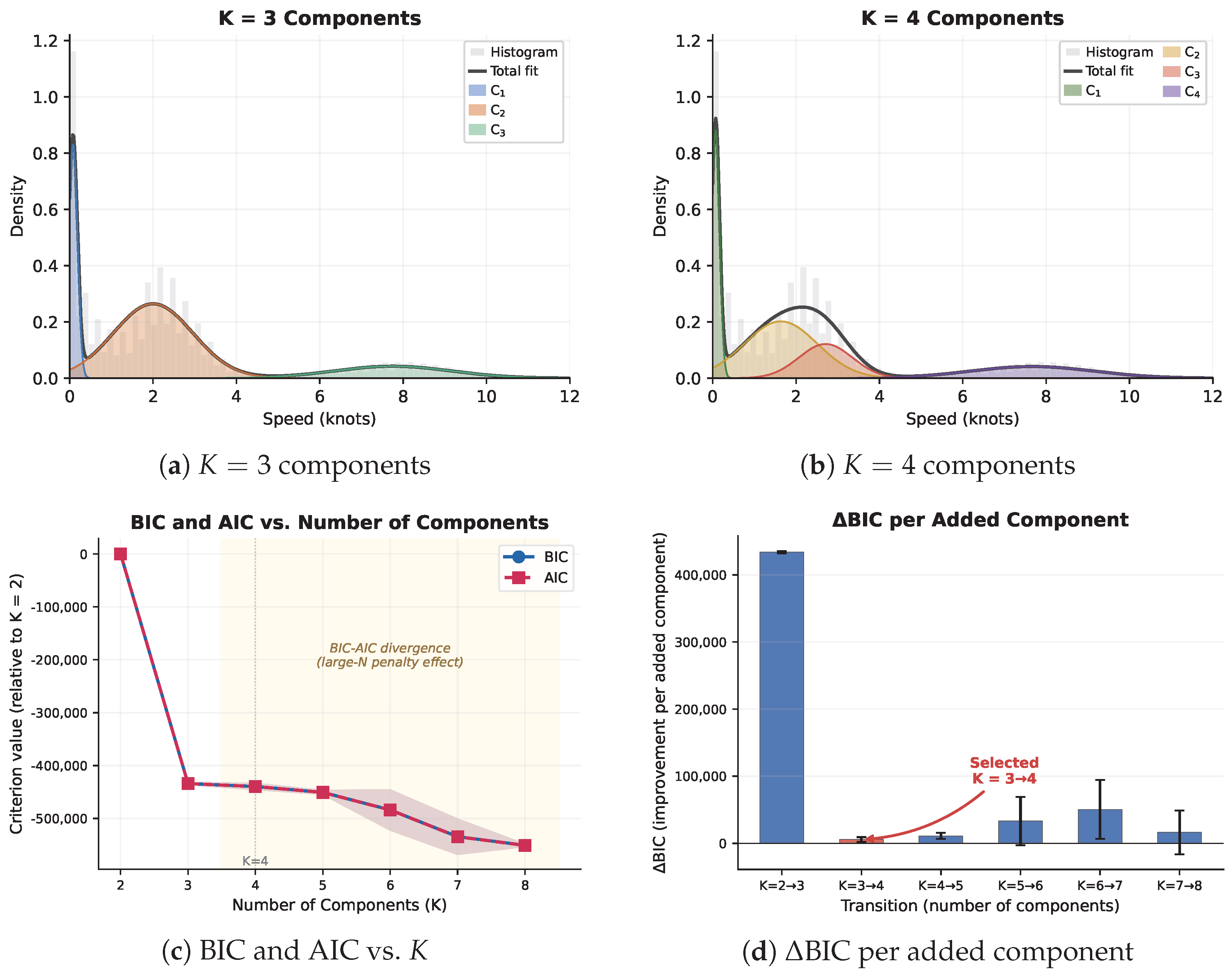
To determine the number of Gaussian components K, we fit mixture models for $K\in \{2,3,\dots ,8\}$ on a stratified sample of 900,000 speed points and evaluate both the Bayesian Information Criterion (BIC) and the Akaike Information Criterion (AIC). As shown in Figure 2c, the BIC curve exhibits its steepest descent at $K=3$, while the $K=3\to 4$ transition yields a comparatively modest $\Delta \mathrm{BIC}$ (Figure 2d). Figure 2d displays only $\Delta \mathrm{BIC}$; because $\Delta \mathrm{AIC}=\Delta (-2lnL)+2\Delta k$ and $\Delta \mathrm{BIC}=\Delta (-2lnL)+klnN\Delta k$ share the same log-likelihood term $\Delta (-2lnL)$, all three criteria agree on the $K=3\to 4$ improvement, and the large-sample BIC–AIC divergence is already visible in Figure 2c. However, the BIC and AIC curves diverge beyond $K\ge 4$, reflecting the well-known tendency of BIC to under-select components at large sample sizes: the BIC penalty per parameter $klnN\approx 13.7k$ substantially exceeds the AIC penalty $2k$. Second, the log-likelihood improvement from $K=3$ to $K=4$ is consistently positive across all five random seeds, confirming that the fourth component captures non-trivial structure in the speed distribution. Third, $K=4$ provides a physically meaningful decomposition: under $K=3$, the low-speed operational range collapses into a single broad mode (Figure 2a), whereas $K=4$ resolves it into two distinct components centered near 0 and 1.6 kts respectively, capturing finer structure in the low-speed range (Figure 2b). We therefore adopt $K=4$ as it balances statistical evidence with distributional resolution.

$$P(C_k\mid x)={\displaystyle \frac{{\pi }_k·\mathcal{N}(x\mid {\mu }_k,{\sigma }_k)}{{\sum }_{j=1}^4{\pi }_j·\mathcal{N}(x\mid {\mu }_j,{\sigma }_j)}}$$

(2)

where $\mathcal{N}(x\mid {\mu }_k,{\sigma }_k)$ denotes the Gaussian probability density function:

$$\mathcal{N}(x\mid {\mu }_k,{\sigma }_k)={\displaystyle \frac{1}{\sqrt{2\pi }{\sigma }_k}}exp\left(-{\displaystyle \frac{{(x-{\mu }_k)}^2}{2{\sigma }_k^2}}\right)$$

(3)

For two adjacent motion states $C_k$ and $C_{k+1}$, the optimal decision boundary $T_k$ is defined, under the Bayesian decision theory framework, as the speed value that equalizes their posterior probabilities:

$$P(C_k\mid x=T_k)=P(C_{k+1}\mid x=T_k),k=1,2,3$$

(4)

Since the denominator of the posterior probability is identical across all components in Equation (2), Equation (4) simplifies to

$${\pi }_k·\mathcal{N}(T_k\mid {\mu }_k,{\sigma }_k)={\pi }_{k+1}·\mathcal{N}(T_k\mid {\mu }_{k+1},{\sigma }_{k+1})$$

(5)

This boundary exhibits clear statistical optimality. To the left of $T_k$, where $P(C_k\mid x)>P(C_{k+1}\mid x)$, assigning a sample to component $C_k$ minimizes the posterior risk; to the right, assigning it to $C_{k+1}$ minimizes the posterior risk. Consequently, $T_k$ serves as the Bayes-optimal split point for separating adjacent motion states.

In practical computation, exactly solving Equation (4) requires solving a quadratic equation in x for each pair of adjacent components. The equal-probability decision boundary can be approximated as the midpoint between the means of two adjacent components:

$$T_k\approx {\displaystyle \frac{{\mu }_k+{\mu }_{k+1}}{2}}$$

(6)

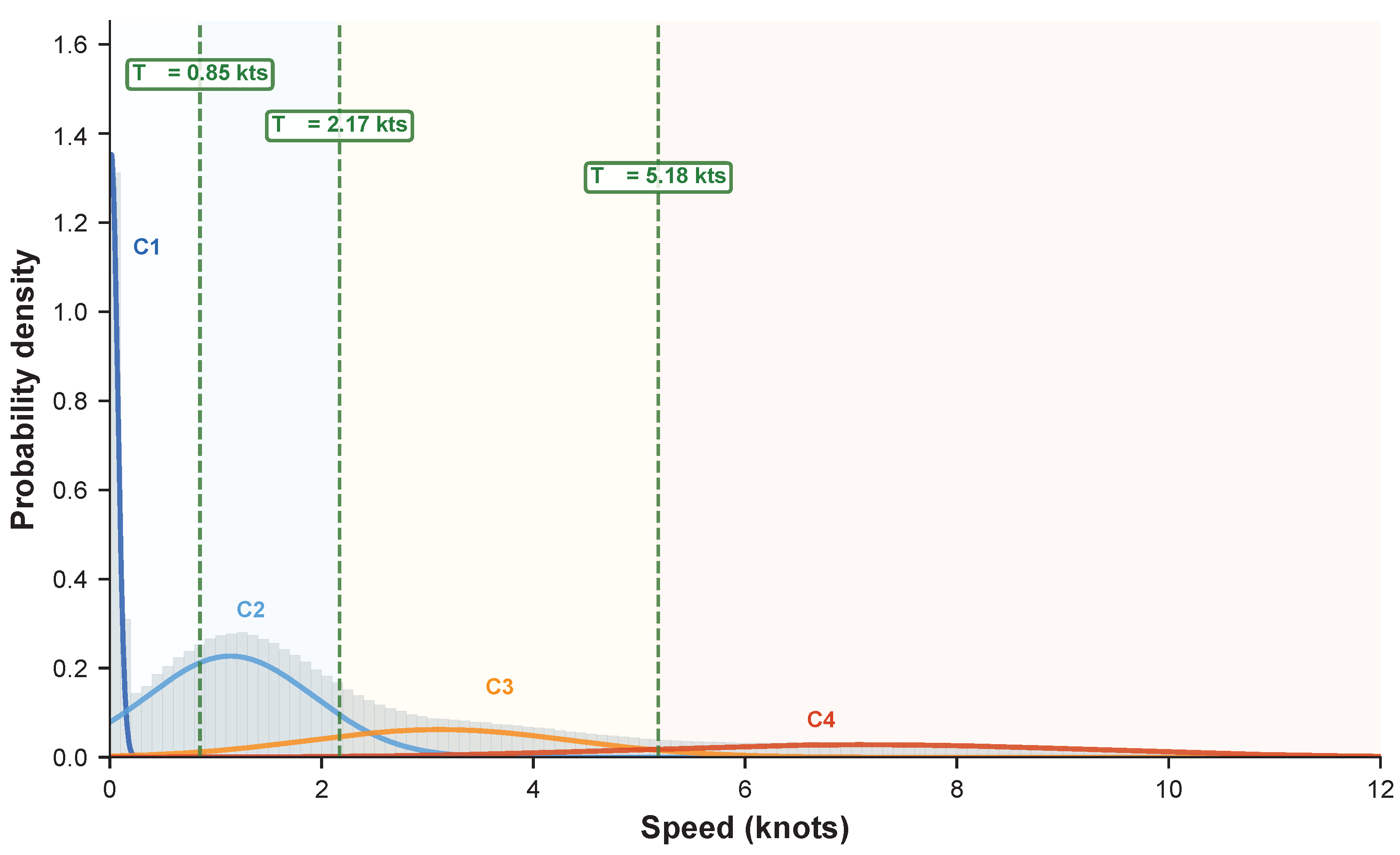
Substituting the component means into Equation (6) yields three speed interval segmentation thresholds. We overlay these thresholds as dividing lines onto the speed frequency histograms of the three fishing vessel categories. As shown in Figure 3, the four colored curves correspond to the four Gaussian components, and the red lines mark the three decision boundaries, namely, 0.85 kts, 2.17 kts, and 5.18 kts, determined by the midpoints of adjacent component means.

2.3. Robust Feature Design

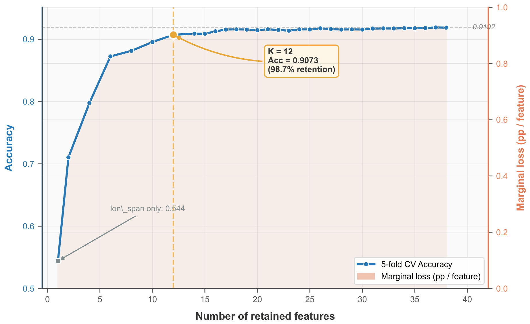
Since the AIS data used in this paper are predominantly sampled at 10 min intervals, the reliability of instantaneous motion details between adjacent points degrades. We therefore construct a 39-dimensional feature set based on window statistics across multiple dimensions, as listed in

Table 1. Composition of the 39-dimensional feature system.

Feature Category	Dim.	Feature Names
Activity range	2	lon_span, lat_span
Displacement distribution	4	delta_lon_median, delta_lon_iqr, delta_lat_median, delta_lat_iqr
Speed interval proportion	4	speed_ratio_[0,0.85), [0.85,2.17), [2.17,5.18), [5.18, $v_{\mathrm{up}}$]
Cumulative turning	3	cumul_turn_mean, cumul_turn_std, cumul_turn_max
Trajectory shape	3	sinuosity, median_dist_to_center, direction_consistency
Stop events	3	stop_count, stop_avg_dur, stop_max_dur
Global speed statistics	4	speed_mean, speed_median, speed_std, speed_iqr
Speed extremes	2	speed_max, speed_min
Speed distribution shape	2	speed_skewness, speed_kurtosis
Motion change rate	4	acc_median, acc_iqr, turn_rate_median, turn_rate_iqr
Heading distribution	2	course_mean, course_concentration
Spatial shape	6	bbox_aspect_ratio, speed_autocorr_lag1, stop_spatial_entropy, turn_point_density, turn_gap_cv, fractal_dim

.

The features listed in Table 1 can be interpreted as follows:

Speed interval proportions: Let the speed sequence be $S=\{s_1,s_2,\dots ,s_n\}$, and let the speed interval thresholds be $0=v_0<v_1<v_2<v_3<v_{\mathrm{up}}=12.0$. The proportion $R_k$ of the k-th interval is defined as

$$R_k={\displaystyle \frac{1}{n}}{\displaystyle \sum _{i=1}^n}\mathbb{I}(v_{k-1}\le s_i<v_k),k=1,\dots ,4$$

(7)

where $\mathbb{I}(·)$ is the indicator function, equal to 1 if the condition holds and 0 otherwise; the four proportions always sum to 1 and represent the fraction of time the fishing vessel spends in each of the four motion states.

Global speed statistics, speed extremes, and speed distribution shape: The global speed statistics include the mean, median, standard deviation, maximum, minimum, and interquartile range, while the speed distribution shape is captured by skewness and kurtosis:

$$g_1={\displaystyle \frac{\frac{1}{n}{\sum }_{i=1}^n{(s_i-\overline{s})}^3}{{\left(\frac{1}{n}{\sum }_{i=1}^n{(s_i-\overline{s})}^2\right)}^{3/2}}},g_2={\displaystyle \frac{\frac{1}{n}{\sum }_{i=1}^n{(s_i-\overline{s})}^4}{{\left(\frac{1}{n}{\sum }_{i=1}^n{(s_i-\overline{s})}^2\right)}^2}}-3$$

(8)

A positive $g_1$ indicates a right-skewed distribution, reflecting a prevalence of higher speed values, whereas a negative $g_1$ indicates a left-skewed distribution with a prevalence of lower speed values. A positive $g_2$ corresponds to a distribution that is more peaked than the normal distribution, while a negative $g_2$ indicates a flatter distribution.

Cumulative turning: Let n be the number of trajectory points and $W=6$ the sliding window size. For the k-th window, the cumulative turning angle is defined as the sum of absolute heading differences over all adjacent point pairs within the window:

$$C_k={\displaystyle \sum _{j=k}^{k+W-2}}\Delta \theta (c_j,c_{j+1})$$

(9)

where $c_j$ is the course over ground of the j-th trajectory point, and $\Delta \theta (c_j,c_{j+1})$ is the minimum absolute heading difference between the two points (ranging in $[0°,180°]$). Because AIS course over ground is reported in the range $[0°,360°)$, a naïve subtraction $|c_j-c_{j+1}|$ would introduce an artificial discontinuity at the 360°/0° boundary. To avoid this, we define the minimum angular difference as

$$\Delta \theta (\alpha ,\beta )=min\left((\alpha -\beta )mod360°,360°-(\alpha -\beta )mod{360}^{°}\right)$$

(10)

which always yields a value in $[0°,180°]$ and is free of boundary artifacts.

By iterating over all $N_W=n-W+1$ windows, we extract the mean, standard deviation, and maximum of the cumulative turning sequence.

For the heading distribution features, we adopt a sin/cos decomposition that respects the circular topology, which representation maps angles onto the unit circle and thus introduces no artificial discontinuity at the 360°/0° boundary. Given a sequence of course values $\{c_1,c_2,\dots ,c_n\}$, the circular mean is computed as $\overline{c}=\mathrm{atan}2(\overline{sinc},\overline{cosc})$ and the circular concentration as $R=\sqrt{{\overline{sinc}}^2+{\overline{cosc}}^2}$, where the overline denotes the arithmetic mean.

Trajectory shape: This category includes three features: sinuosity, median distance to the center point, and head-to-tail direction consistency.

Sinuosity is defined as the ratio of the total path length to the straight-line distance between the start and end points:

$$S={\displaystyle \frac{{\sum }_{i=1}^{N-1}{d}_{\mathrm{haversine}}(p_i,p_{i+1})}{d_{\mathrm{haversine}}(p_1,p_N)}}$$

(11)

where $p_i=({\mathrm{lon}}_i,{\mathrm{lat}}_i)$ denotes the i-th trajectory point, $d_{\mathrm{haversine}}$ is the spherical distance, and N is the total number of trajectory points. A sinuosity value of $S=1$ indicates a strictly straight trajectory, while $S>1$ indicates tortuous movement.

Head-to-tail direction consistency is defined using the same minimum angular difference $\Delta \theta$ introduced above, applied to the heading vector of the first segment ($p_1\to p_2$) and that of the last segment ($p_{N-1}\to p_N$), and normalized to the interval $[0,1]$:

$$C_{\mathrm{dir}}=1-{\displaystyle \frac{|\Delta \theta |}{{180}^{°}}}$$

(12)

where $C_{\mathrm{dir}}=1$ indicates that the head and tail headings are perfectly consistent, while $C_{\mathrm{dir}}=0$ indicates completely opposite headings.

Stop events: We adopt the low-speed threshold $T_1=0.85$ kts and define a stop event as a sequence of at least two consecutive sampling points with speed below $T_1$. The duration of each stop event is measured in number of trajectory points, from which we extract the total number of stop events, the average duration in points, and the maximum duration in points.

Motion change rate: Acceleration and turn rate are defined as follows:

$$a_i={\displaystyle \frac{s_{i+1}-s_i}{\Delta t_i+ϵ}}$$

(13)

$$r_i={\displaystyle \frac{\Delta \theta (c_i,c_{i+1})}{\Delta t_i+ϵ}},i=1,2,\dots ,n-1$$

(14)

where $\Delta t_i=t_{i+1}-t_i$ is the time difference between adjacent points, and $ϵ={10}^{-6}$ is a small smoothing term to prevent division by zero. We then extract the median and interquartile range of the acceleration sequence $\left\{a_i\right\}$ and the turn rate sequence $\left\{r_i\right\}$.

Fractal dimension: We adopt the box-counting method. At multiple scales $ϵ$, we cover the trajectory with a grid and count the number of grid cells $N\left(ϵ\right)$ intersected by the trajectory. The slope is then fitted via the log–log linear relationship:

$$D_{\mathrm{box}}={\displaystyle \frac{\Delta logN\left(ϵ\right)}{\Delta log(1/ϵ)}}$$

(15)

Using five scales $ϵ\in \{0.005°,0.01°,0.02°,0.05°,0.1°\}$, we perform a least-squares linear fit on $(log(1/ϵ),logN(ϵ\left)\right)$, and the slope gives the fractal dimension. $D_{\mathrm{box}}\in [1,2]$, with values closer to 1 indicating a more straight-line trajectory and values closer to 2 indicating higher space-filling capacity.

Stop point spatial entropy: The trajectory’s spatial extent is partitioned into a uniform $G\times G$ grid ($G=4$), and the frequency distribution $p_k$ of stop points in each grid cell is computed to calculate the Shannon entropy:

$$H_{\mathrm{stop}}=-\sum _{k:p_k>0}{p}_{k}log(p_k+ϵ)$$

(16)

where $ϵ={10}^{-9}$ is a small smoothing term to prevent $log0$. A larger $H_{\mathrm{stop}}$ indicates a more uniform spatial distribution of stop points, whereas a smaller value indicates that stop points are concentrated in fewer locations.

Turn point density and gap coefficient of variation: A turn point is defined as the position of a trajectory point where the minimum angular difference $\Delta \theta (c_i,c_{i+1})$ between consecutive headings exceeds a threshold $\tau =30°$. Turn point density is defined as the number of turns per unit distance traveled:

$${\rho }_{\mathrm{turn}}={\displaystyle \frac{N_{\mathrm{turn}}}{D_{\mathrm{total}}+ϵ}}$$

(17)

where $D_{\mathrm{total}}={\sum }_{i=1}^{n-1}d(p_i,p_{i+1})$ is the total distance traveled along the trajectory. Let $\{i_1,i_2,\dots ,i_{N_{\mathrm{turn}}}\}$ be the sequence of turn point indices, with $N_{\mathrm{turn}}\ge 3$, and let $\Delta k_j=i_{j+1}-i_j$ denote the index gap between consecutive turn points. The coefficient of variation of these gaps is

$${CV}_{\mathrm{gap}}={\displaystyle \frac{{\sigma }_{\Delta k}}{\overline{\Delta k}+ϵ}}$$

(18)

A larger ${CV}_{\mathrm{gap}}$ indicates a more uneven distribution of turn points, whereas a smaller value indicates a more uniform distribution.

Speed autocorrelation: The persistence of speed over time is measured by the first-order autocorrelation coefficient:

$${\rho }_1={\displaystyle \frac{{\sum }_{i=1}^{n-1}(s_i-\overline{s})(s_{i+1}-\overline{s})}{{\sum }_{i=1}^n{(s_i-\overline{s})}^2+ϵ}}$$

(19)

where $\overline{s}$ is the mean speed, and $ϵ={10}^{-9}$ is a small smoothing term to prevent division by zero. A value of ${\rho }_1\to 1$ indicates that the speed remains persistent and stable with high positive correlation, whereas ${\rho }_1\to -1$ indicates rapid alternating changes in speed. When $n<4$ or the standard deviation of speed is zero, a default value of 0 is assigned.

2.4. Classification Model and Evaluation Strategy

2.4.1. Light Gradient Boosting Machine (LightGBM)

This paper adopts LightGBM [19] as the classification model for fishing vessel operation types. LightGBM is an efficient ensemble learning algorithm based on gradient boosting decision trees, which integrates two core optimization techniques: Exclusive Feature Bundling (EFB) and gradient-based one-side sampling (GOSS). EFB is theoretically framed as a graph coloring problem and bundles mutually exclusive features in high-dimensional sparse data with little or no loss, effectively reducing feature dimensionality and the memory overhead of histogram construction. GOSS is based on the key observation that samples with larger absolute gradients contribute more to model training; it retains all high-gradient samples and randomly samples low-gradient ones, thereby significantly accelerating training without traversing the full dataset. The pseudocode of the training process is presented in Algorithm 1.

Algorithm 1 LightGBM Training Procedure

Input:  Training set $\mathcal{D}={\left\{(x_i,y_i)\right\}}_{i=1}^N$, number of iterations M, learning rate $\eta$, number of leaves L, minimum leaf samples $n_{min}$ Output:  Ensemble model $f_M\left(x\right)$   1: Initialize $f_0\left(x\right)=arg{min}_c{\sum }_{i=1}^{N}L(y_i,c)$   2: Use graph coloring to bundle mutually exclusive features with EFB, obtaining the reduced feature set $\tilde{\mathcal{D}}$   3: for$m=1$to  M  do   4:   for $i=1$to N do   5:    $g_i^{\left(m\right)}\leftarrow {\left[{\displaystyle \frac{\partial L(y_i,\widehat{y})}{\partial \widehat{y}}}\right]}_{\widehat{y}=f_{m-1}\left(x_i\right)}$   6:   end for   7:   Sort in descending order by $|g_i^{\left(m\right)}|$, retain the top $a\times 100\%$ (large gradient) samples   8:   Randomly sample $b\times 100\%$ from the remaining $(1-a)\times 100\%$ (small gradient) samples, weight ${\displaystyle \frac{1-a}{b}}$   9:   Combine to obtain the training subset ${\mathcal{D}}_m$ for this round 10:   Train a decision tree $h_m\left(x\right)$ on ${\mathcal{D}}_m$ by maximizing information gain, with leaf-wise growth: 11:      Select the leaf with the maximum gain from all current leaves to split 12:      Tree complexity is controlled by L and $n_{min}$ 13:   $f_m\left(x\right)\leftarrow f_{m-1}\left(x\right)+\eta ·h_m\left(x\right)$ 14:   if Validation loss does not decrease for k consecutive rounds then 15:    break 16:   end if 17: end forreturn$f_M\left(x\right)=f_0\left(x\right)+{\sum }_{m=1}^M\eta ·h_m\left(x\right)$

We adopt a Bayesian optimization method based on the Tree-structured Parzen Estimator (TPE), implemented via the Optuna framework [20], and conduct 50 trials on a fixed 3-fold stratified cross-validation split. The search ranges and the final optimal values of each hyperparameter are presented in

Table 2. LightGBM hyperparameter search ranges and optimal values.

Parameter	Description	Search Range	Optimal Value
num_leaves	Number of leaves	[15, 63]	62
learning_rate	Learning rate	[0.01, 0.1]	0.076
feature_fraction	Feature sampling fraction	[0.6, 0.9]	0.757
bagging_fraction	Bagging sampling fraction	[0.6, 0.9]	0.892
bagging_freq	Bagging frequency	[1, 10]	10
min_child_samples	Minimum child samples	[5, 50]	15

.

2.4.2. Evaluation Strategy and Metrics

We adopt a two-tier evaluation strategy. First, the full dataset is stratified and randomly split into 70% training and 30% test sets; the test set is used to assess the model’s generalization performance. Second, 5-fold stratified cross-validation is employed to obtain the mean and standard deviation of performance across different data splits, so as to examine model stability.

Model performance is evaluated using the following metrics. Let $K=3$ be the total number of classes, and ${\mathrm{TP}}_k$, ${\mathrm{FP}}_k$, ${\mathrm{FN}}_k$ denote the numbers of true positives, false positives, and false negatives for class k, with N being the total sample size.

Accuracy measures the proportion of correctly classified samples across all classes:

$$\mathrm{Accuracy}={\displaystyle \frac{{\sum }_{k=1}^K{\mathrm{TP}}_k}{N}}$$

(20)

Precision and Recall for each class respectively measure the proportion of true positive predictions among all predictions for class k and the proportion of actual class k samples that are correctly identified:

$${\mathrm{Precision}}_k={\displaystyle \frac{{\mathrm{TP}}_k}{{\mathrm{TP}}_k+{\mathrm{FP}}_k}},{\mathrm{Recall}}_k={\displaystyle \frac{{\mathrm{TP}}_k}{{\mathrm{TP}}_k+{\mathrm{FN}}_k}}$$

(21)

$F_1$ score is the harmonic mean of precision and recall for class k:

$$F_1^{\left(k\right)}=2·{\displaystyle \frac{{\mathrm{Precision}}_k·{\mathrm{Recall}}_k}{{\mathrm{Precision}}_k+{\mathrm{Recall}}_k}}$$

(22)

Macro-averaged precision, macro-averaged recall, and macro-averaged $F_1$ score are obtained by taking the arithmetic mean of the corresponding per-class metrics and are unaffected by class imbalance:

$$\text{Macro-}P={\displaystyle \frac{1}{K}}{\displaystyle \sum _{k=1}^K}{\mathrm{Precision}}_k,\text{Macro-}R={\displaystyle \frac{1}{K}}{\displaystyle \sum _{k=1}^K}{\mathrm{Recall}}_k,\text{Macro-}{F}_1={\displaystyle \frac{1}{K}}{\displaystyle \sum _{k=1}^K}{F}_1^{\left(k\right)}$$

(23)

Kappa coefficient measures the agreement between the classification results and a random classification:

$$\kappa ={\displaystyle \frac{p_o-p_e}{1-p_e}}$$

(24)

where $p_o=\mathrm{accuracy}$ is the observed agreement, and $p_e={\sum }_{k=1}^K{\displaystyle \frac{({\mathrm{TP}}_k+{\mathrm{FP}}_k)({\mathrm{TP}}_k+{\mathrm{FN}}_k)}{N^2}}$ is the expected agreement.

3. Results

3.1. Classification Performance of the 39-Dimensional Feature System

Following the evaluation methodology described above, we assess the classification performance of the 39-dimensional features through 5-fold stratified cross-validation, All experiments were conducted on a workstation equipped with an Intel Core i7-12700H processor (Intel, Santa Clara, CA, USA) and an NVIDIA GeForce RTX 3060 Laptop GPU (NVIDIA, Santa Clara, CA, USA), running Python 3.9 with PyTorch 2.8.0 (CUDA 12.6). The resulting performance is presented in

Table 3. Experimental results of the 39-dimensional feature system.

Accuracy	Macro-F1	Kappa	Gillnet F1	Purse Seine F1	Trawler F1
0.9192 ± 0.0024	0.9191 ± 0.0025	0.8788 ± 0.0036	0.959 ± 0.003	0.886 ± 0.003	0.912 ± 0.004

.

The results show that the model with the 39-dimensional feature system achieves an average accuracy of 91.92% under 5-fold stratified cross-validation (Macro-F1 = 0.9191, Kappa = 0.8788). The low standard deviations across folds for all metrics indicate highly consistent performance across different data splits, with no evidence of overfitting. However, the F1 scores of the three classes exhibit a clear hierarchical differentiation: gillnet reaches an F1 of 0.959 and is almost perfectly separable, as its near-zero speed stopping behavior provides sufficient discriminative signal in the feature space; trawler obtains an F1 of 0.912; purse seiner obtains the lowest F1, only 0.886.

3.2. Confusion Matrix Analysis

Although the overall model performance has reached a high level, a significant imbalance in classification performance persists across different classes. The relatively lower F1 scores of purse seine and trawler indicate persistent bidirectional misclassification between the two. To systematically diagnose the specific patterns of classification error, this section presents the confusion matrix in Figure 4 to analyze the model’s predictions. In the confusion matrix, each row corresponds to the true class, each column to the predicted class, the diagonal elements represent the recall for each class, and the off-diagonal elements reveal the direction and proportion of misclassification between classes.

In Figure 4, 153 purse seine samples are misclassified as trawler, accounting for 8.4% of the purse seine samples; 151 trawler samples are misclassified as purse seine, accounting for 8.1% of the trawler samples. Gillnet achieves the highest classification accuracy, reaching 97.4%.

The confusion matrix reveals a persistent bidirectional misclassification between purse seine and trawler. In practice, the two vessel types exhibit clearly different operational patterns: trawlers predominantly move in straight lines along isobaths during towing [21], whereas purse seiners perform circular encircling maneuvers to surround fish schools and subsequently drift at low speed during net hauling. Under high-frequency sampling, these behavioral differences would produce different trajectory signatures. However, at the 10 min sampling interval of the AIS data used in this study, a circular encircling maneuver may be captured by only a few widely spaced points that approximate straight-line segments, as shown in Figure 5 and Figure 6. Consequently, the windowed statistics computed over these sparsely sampled trajectories yield overlapping feature distributions for the two classes.

To further diagnose the origin of the per-class F1 hierarchy, we quantify the geometry of the three classes in the standardized 39-dimensional feature space. The Euclidean distance between class centroids reveals that the purse seine–trawler pair is separated by only 2.247, less than half the gillnet–purse seine distance (4.034) or the gillnet–trawler distance (4.388). The mean cross-class pairwise distance confirms this pattern: purse seine–trawler yields 7.007, whereas the gillnet–purse seine and gillnet–trawler pairs yield 8.780 and 8.795, respectively. Thus, purse seine and trawler have substantially overlapping regions of the feature space.

We further compute the per-feature Fisher discriminant ratio, a univariate separability metric between the purse seine–trawler pair, to identify which individual features contribute to the difficulty of this class boundary. Among the 39 features, the near-zero Fisher ratios for acceleration-related features are a direct consequence of the 10 min sampling interval: the acceleration $\Delta v/\Delta t$ is attenuated by the long $\Delta t\approx$600 s, compressing all vessel types toward zero. The most discriminative features are $\text{lon\_span}$ (Fisher = 0.61), $\text{speed\_ratio\_}[\mathrm{5.18},\mathrm{12.0}]$ (0.43), and $\text{delta\_lon\_iqr}$ (0.39), reflecting the larger longitudinal search range and higher transit speed of purse seine compared with trawl operations.

3.3. Feature Importance and Feature Ablation

To quantify the contribution of the designed features to model classification, we extract the split importance from the LightGBM classifier trained on the 39-dimensional feature system and rank them in descending order. Figure 7 shows the top 30 features.

As shown in the feature importance ranking in Figure 7, the spatial range features (lon_span and lat_span) have tied importance scores and rank among the top three, with the first place being the interquartile range of latitudinal displacement (delta_lat_iqr). From the perspective of fishing behavior, trawlers typically conduct reciprocating sweep operations within a relatively concentrated spatial range, whereas purse seiners need to search over a wider area based on the distribution of fish schools and consequently show greater latitudinal displacement variation.

Among the speed interval proportion features, speed_ratio_2.17_5.18 and speed_ratio_0.85_2.17 rank 5th and 6th, respectively, whereas speed_ratio_0.00_0.85 and speed_ratio_5.18_$v_{\mathrm{up}}$ rank relatively lower in importance, indicating that the operation patterns of different fishing vessels exhibit high homogeneity during low-speed and high-speed navigation phases.

Although the full-feature model already offers reasonable inference efficiency, to verify the compactness of the feature set and quantify the independent contribution of each feature category, this paper achieves lightweight design through feature dimension compression. Specifically, we perform backward ablation by removing features in ascending order of their importance: at each step, the currently least important feature is discarded and the 5-fold cross-validation accuracy is re-evaluated, thereby constructing a complete trade-off curve from a single feature to the full system. This allows us to determine the critical number of feature dimensions at which the marginal accuracy gain plateaus. The results are shown in Figure 8 and

Table 4. Key points of sequential feature ablation (5-fold CV).

Retained Features	Accuracy	Macro-F1	Accuracy Retention	Feature Compression Rate
39	0.9192	0.9191	100.0%	0%
14	0.9091	0.9090	98.9%	64.1%
12	0.9073	0.9073	98.7%	69.2%
10	0.8956	0.8955	97.4%	74.4%
8	0.8816	0.8813	95.9%	79.5%
4	0.7978	0.7978	86.8%	89.7%
1	0.5441	0.5230	59.2%	97.4%

.

In Figure 8, the curve shows the 5-fold cross-validation accuracy as a function of the number of retained features, with the horizontal dashed line marking the baseline accuracy of the 39-dimensional system. The right axis indicates the average accuracy loss per feature removed between consecutive ablation steps (in percentage points per feature).

The curve increases overall from left to right and plateaus at $K=17$. At $K=12$, a total of 27 features have been removed, yet the accuracy drops by only 1.19%, achieving a feature compression ratio of 69.2% while retaining 98.7% of the accuracy.

3.4. Multi-Model Performance Comparison

The generalization ability of a feature set is reflected not only in the performance stability under the same classifier but also in the consistency of performance across different classification algorithms, meaning that regardless of which mainstream classifier is adopted, models trained on this feature set should achieve similarly excellent performance. To this end, this section selects several representative classification algorithms for comparative experiments: XGBoost [22], Random Forest [23], SVM [24], and LSTM. All models adopt the identical 5-fold stratified cross-validation protocol and the full feature matrix. The results obtained through 5-fold cross-validation are listed in

Table 5. Performance comparison of different machine learning algorithms.

Model	Accuracy	Macro-F1	Training Time (s)	Inference Time (s)
LightGBM	0.9192 ± 0.0024	0.9191 ± 0.0025	12.18 ± 1.80	0.051 ± 0.007
XGBoost	0.9152 ± 0.0032	0.9151 ± 0.0033	13.97 ± 2.26	0.059 ± 0.018
Random Forest	0.9086 ± 0.0039	0.9084 ± 0.0040	17.03 ± 2.08	0.146 ± 0.021
SVM (RBF)	0.8931 ± 0.0033	0.8927 ± 0.0033	1.76 ± 0.03	1.230 ± 0.280
LSTM	0.8992 ± 0.0180	0.8992 ± 0.0180	4520 ± 820	0.003 ± 0.002

.

The evaluation results show that all three tree-based classifiers exceed 90% accuracy on the same 39-dimensional feature set with low cross-validation variance, while the remaining classifiers also achieve accuracy approaching 90%, validating the effectiveness of the proposed robust feature design. Among them, LightGBM achieves the highest accuracy (91.92%) and Macro-F1 (0.9191) with the smallest variance and the shortest training time among tree-based models. Although SVM has the shortest overall training time (1.76 s), its accuracy is the lowest at 89.31%. Although LSTM is theoretically capable of learning temporal dependencies, its cross-validation standard deviation (±0.0180) is approximately 7.5 times that of LightGBM, suggesting that the sparse data input and irregular temporal structure fail to provide sufficiently reliable sequential signals for effective recurrent learning.

To further demonstrate the advantage of LightGBM with handcrafted features, we evaluated an LSTM encoder and a pre-LN Transformer encoder with learnable positional encoding on a stratified subsample of 2400 trajectories. All three model families were evaluated on identical 5-fold cross-validation splits. The results are summarized in

Table 6. Performance comparison on the 2400-sample stratified subsample (5-fold CV).

Model	Accuracy	Macro-F1	Training Time (s/fold)
LightGBM	0.8912 ± 0.0040	0.8910 ± 0.0038	19.5 ± 4.9
Transformer	0.8525 ± 0.0137	0.8495 ± 0.0166	2235 ± 842
LSTM	0.8338 ± 0.1226	0.8149 ± 0.1609	535 ± 192

.

LightGBM with the 39-dimensional feature set achieves an accuracy of 0.8912 ± 0.0040 and a Macro-F1 of 0.8910 ± 0.0038, outperforming both the Transformer (accuracy 0.8525 ± 0.0137, Macro-F1 0.8495 ± 0.0166) and the LSTM (accuracy 0.8338 ± 0.1226, Macro-F1 0.8149 ± 0.1609). The advantage of LightGBM extends beyond accuracy: its cross-validation standard deviation (0.0040) is 3.4 times smaller than that of the Transformer (0.0137) and 30.7 times smaller than that of the LSTM (0.1226), with the latter failing to converge in one of the five folds. In terms of training efficiency, LightGBM requires only 19.5 s per fold, compared with 2,235 s for the Transformer and 535 s for the LSTM. Notably, with less than one-fifth of the full dataset, LightGBM with handcrafted features maintains a competitive accuracy of 89.1%, confirming that the feature system enables robust classification under substantially reduced data conditions.

4. Discussion

4.1. Research Strengths and Innovations

This study addresses the practical constraints that, under 10 min sparse AIS sampling, the reliability of point-wise statistics degrades and interpolation tends to introduce spurious motion patterns. We propose a complete classification framework that avoids interpolation, relies on robust features, and uses data-driven thresholds, by statistical aggregation over trajectory-level windows can preserve behavioral signals that point-to-point variations tend to lose at 10 min intervals, while encoding domain knowledge to reduce the dependence on large labeled datasets that end-to-end models typically require.

Without interpolation, the 39-dimensional feature system achieves a 5-fold cross-validation accuracy of 91.92%, a Macro-F1 of 0.919, and a Kappa of 0.879, with fold-to-fold standard deviations of only 0.002 to 0.004. Ablation experiments further reveal that approximately the top 20% of features retain about 96% of the classification capability. Combining the 12-dimensional lightweight feature subset with LightGBM, which offers the fastest inference and achieves simultaneous compression on both the feature and model sides, constituting an efficient deployment solution.

4.2. Limitations

The AIS data used in this study are drawn exclusively from a single fishing ground in the East China Sea (21° N–37° N, 115° E–130° E), and their cross-region generalization capability has not been verified. The ground truth is derived from fishery registration information, and discrepancies may exist between the registered operation type and the actual behavior at sea. Such label noise could lead to an underestimation of the model’s true discriminative ability; this study does not quantify the extent of label noise.

4.3. Findings and Future Recommendations

The multi-model comparison demonstrates that, under 10 min sparse sampling, the inductive bias introduced by handcrafted features yields better fold-to-fold stability than LSTM. However, the LSTM was not explored within a thoroughly tuned deep learning framework that integrates handcrafted features with end-to-end learning. The consistently high accuracy across different tree-based models further confirms that feature robustness, rather than model choice, is the primary source of performance. The optimal composition of the 12-dimensional lightweight feature subset may vary with fishing ground and sampling conditions, and its statistical stability across scenarios remains to be examined. Furthermore, extracting auxiliary screening signals for registration–behavior discrepancies from systematic inconsistencies between registered labels and model predictions could serve as a valuable direction for subsequent research.

5. Conclusions

This paper addresses the problem of fishing vessel type classification under sparse AIS data and proposes a complete classification framework that requires no interpolation, relies on robust features, and adopts data-driven thresholds. The method is systematically validated on 18,320 fishing vessel trajectories in the East China Sea. Without interpolation, the framework achieves a cross-validation accuracy of 91.92% (Macro-F1 = 0.919, Kappa = 0.879), with fold-to-fold standard deviations of only 0.002 to 0.004. The adaptive speed thresholds are grounded in the theoretical framework of Bayesian decision boundaries: the optimal splits are determined at points where the posterior probabilities of adjacent motion states are equal, eliminating the need for manual setting and removing the dependence on fishery domain knowledge for speed interval partitioning, thereby providing an adaptive foundation for cross-fishery region transfer. The marginal accuracy decay pattern established by the ablation experiments allows a 12-dimensional feature subset to retain 98.7% of the accuracy with a compression ratio of 69%. The handcrafted feature design is further justified by the 10 min sparse sampling constraint, under which behavioral signals in raw coordinate sequences are substantially attenuated; end-to-end models struggle to extract discriminative patterns from such degraded inputs, whereas statistical aggregation in the feature system preserves these signals while encoding domain knowledge to reduce dependence on large labeled datasets.