Optimization of Human–Machine Interface Layout for Mechanical Support Position of Manned Submersibles Based on a Task-Information Network Approach

Abstract

The human–machine interface (HMI) of the mechanical support (MS) position (MS-HMIs) of manned submersibles features multiple screens, information-rich displays, and complex operational logic, which can reduce operator efficiency, increase cognitive load, and lead to human errors. The layout determines the perception of information density, complexity, and logic, making the optimization of the HMI layout highly significant. To address this issue, a layout optimization approach is proposed based on a task-information network integrating multi-objective optimization. First, the basic MS-HMI elements are decomposed, and Hierarchical Task Analysis (HTA) is used to construct task sequences and element usage sequences. The Space-P and Space-L methods are applied to build the task–information network, based on which element grouping and importance are determined through network topology analysis. Incorporating ergonomic layout principles, a multi-objective optimization model is formulated and solved using the NSGA-II algorithm to generate feasible optimized layouts. Experimental verification results demonstrate that the optimized interfaces significantly outperform the original design in terms of operational performance, eye-tracking metrics, and subjective evaluations. Operation duration and task completion time decreased by over 6%, average saccade speed was reduced by up to 17.1%, and subjective ratings improved substantially. By integrating complex network analysis, typical submersible task sequences, and ergonomic principles, this study presents a systematic, evidence-based, effective, and task-compliant method for optimizing HMI layouts.

1. Introduction

The console of a manned submersible is an important channel for operators to obtain information, make decisions, and execute commands. The mechanical support position is a typical role within a manned submersible, responsible for ensuring the safe operation of the submersible’s mechanical system. Its primary duties include monitoring of the submersible’s attitude and depth and the status of various valves and control systems to ensure smooth operation under various working conditions. Facing the rapidly changing underwater environment, operators need to continuously monitor a large amount of updated real-time information on the human–machine interface (HMI). In emergency situations, operators must be able to quickly identify and analyze abnormal information, make decisions, and provide accurate and timely responses to ensure stable operation. With the development of HMIs, the need for traditional tasks is gradually decreasing. However, operators still face a relatively high workload [1]. This challenge is not unique to submersibles: studies on maritime operator workload have demonstrated that information-intensive multi-screen displays in safety-critical marine environments significantly increase cognitive demands and the risk of human error [2]. Relevant research shows that by optimizing the layout of the HMI, it is possible to reduce human error, lower mental workload, and improve visual search efficiency and comfort [3,4,5,6,7]. Therefore, it is necessary to conduct research on the optimization of human–machine interface layouts.

At present, research on the optimization of layout mainly focuses on the theoretical exploration of principles such as static operation panels and display- and control-component layouts. In the early days, research was mainly conducted through expert scoring or experience [8,9]. With the development of technology, statistical data metrics such as usage frequency, usage order, and error factors began to serve as an objective basis [10,11]. Later, researchers gradually introduced mathematical models such as the TOPSIS method [12], the multi-criteria method [13,14] and the GEM-AHP method [15]. In the maritime and naval engineering domain, related work has addressed the optimization of cabin-equipment layout using human reliability analysis and multi-objective algorithms [16], and submarine interface design has been explored from the perspective of cognitive work analysis [17]. Studies on deep-sea submersible HMIs have further examined human reliability evaluation [7] and the effects of automation levels on operator performance [4,18]. Static operation panels and display and control components involve less information complexity and are easier to operate. However, in MS-HMIs, there are multiple interfaces with complex and variable information, and the types of operation tasks are diverse. These existing methods were developed primarily for interfaces with fewer elements and simpler task structures and have not addressed the multi-screen, information-dense characteristics of submersible HMI layouts. Practical optimization methods need to be established for the complex characteristics of MS-HMIs.

Complex network theory serves as an effective tool for studying complex systems [19] and has been widely applied in the field of ergonomics. Some studies construct various network models, such as information, task, and social networks, to analyze critical nodes and information flow patterns, thereby optimizing human–machine systems and enhancing their efficiency and reliability. Stanton et al. [20] constructed social, task, and information networks to identify key nodes and load issues in information transfer, providing a basis for optimizing team collaboration [21,22,23]. While EAST operates at the level of team cognition and inter-agent information flow, the present study focuses on intra-interface element relationships for single-operator layout optimization, representing a complementary but distinct application of network-based analysis. Zheng et al. [24] built human–machine interaction information networks based on different granularities, offering insights for improving the reliability of human–machine interaction systems through the optimization of display- and control-device layouts. Wang et al. [25,26] proposed a method for constructing complex networks of aircraft cockpit display and control devices based on expert evaluations and objective experiments. Through community analysis, they revealed the associations between devices, providing a foundation for cockpit layout optimization. As a complex system of submersibles, the HMI can benefit from complex network theory as an effective and reliable approach for layout optimization.

Existing studies have employed different network modeling methods, each with distinct emphases. Zheng et al. [24] and Wu et al. [27] constructed networks utilizing the Space-P method, which focuses on the close connections between information elements but fails to reflect the logical relationships within tasks. In contrast, Wang et al. [28] adopted the Space-L method, which emphasizes the logical associations of tasks but results in a sparser network structure, potentially weakening the relationships between basic elements. These limitations suggest that neither method alone is sufficient to comprehensively characterize the complex relationships among interface elements, including their usage frequency, operation sequences, and logical connections within task sequences. Furthermore, existing research has yet to systematically transform network topology outcomes into quantitative inputs for a multi-objective layout optimization framework, leading to less objective outcomes in interface layout optimization. This gap is particularly pronounced in the context of manned submersible HMIs, where multi-screen displays, diverse task types, and safety-critical operational requirements impose demands that go beyond those addressed by existing methods. Therefore, this study proposes an integrated task-information network approach that combines the Space-P and Space-L methods to comprehensively characterize element relationships and systematically transforms the resulting network topology characteristics into a multi-objective optimization framework incorporating ergonomic design principles, with specific application to the mechanical support position of manned submersibles.

This paper proposes a method based on complex network theory to reformulate the optimization problem of complex MS-HMIs as a multi-objective optimization framework. Owing to the complex information structure and diverse tasks associated with the MS position, the Space-P and Space-L methods are integrated with Hierarchical Task Analysis (HTA) to construct a task-information network. The characteristics of the resulting network topology provide the mathematical foundation for the multi-objective optimization problem. The novelty of this work lies in three aspects: (1) integrating Space-P and Space-L networks into a unified task-information network that captures both co-occurrence and sequential relationships among interface elements; (2) systematically transforming network topology outcomes into mathematical constraints and objective functions for NSGA-II optimization; and (3) providing experimental verification of the optimized layouts in terms of operational performance, eye-tracking metrics, and subjective evaluations through a submersible simulation experiment.

2. Methods

2.1. Layout Design Principles

The HMI of a manned submersible serves as the central hub for command and control, and the mechanical support (MS) position includes two sub-interfaces: the attitude control interface (ACI) and the ups-and-downs control interface (UDCI) [18,29]. The typical tasks of the MS position include five items: heel-angle adjustment, trim-angle adjustment, emergency depth change, monitoring of navigation status, and monitoring of equipment status. When performing tasks, operators need to frequently switch between these two interfaces through the taskbar to obtain information, faced with challenges such as poor structure, intermittence, and interference. These issues can reduce work efficiency, increase cognitive load, and easily result in safety incidents. Therefore, it is essential to analyze and study the HMI, optimize its layout design, and thereby enhance the operational efficiency and safety levels.

The HMI is composed of multiple basic elements, each of which represents the smallest unit for operation or information viewing. The collection of these basic elements is denoted as $E=\{e_1,e_2,\dots e_k\}$, where k is the total number of basic elements. Each basic element can be regarded as a rectangle with fixed dimensions, with its length and width denoted as $w_i$ and $h_i$, respectively. The layout information can be represented by a vector consisting of the coordinates $(x_i,y_i)$ and dimensions of the basic elements, as shown in Equation (1)

$$L=\left\{\left.(x_i,y_i,w_i,h_i)\right|i=1,2,\dots ,n\right\}$$

(1)

The basic elements in the interface encompass all operational and informational display units. By optimizing the positional coordinates of these basic elements, the layout of the HMI can be effectively optimized.

The HMI layout of a manned submersible must consider ergonomic requirements to reduce operational load and enhance interaction efficiency. The optimization process should incorporate layout principles such as spatial compatibility, hierarchy, proximity compatibility, operational sequence, and the shortest-distance principle. Detailed explanations of these principles are provided in

Table 1. Summary of HMI layout design principles.

Layout Principle	Description
Spatial Compatibility	Mutual interference and overlap among all basic elements should be avoided, and a minimum margin should be maintained between all basic elements and the boundaries of the interface.
Hierarchy	Basic elements with high importance and frequent usage should be positioned within the optimal visual range of the human eye or the optimal operational range of the hand.
Proximity Compatibility	Basic elements with high correlation or consistent functionality should be arranged adjacent to or in close proximity to each other.
Operation Sequence	Basic elements of the interface used during the operation process must be positioned relative to the operational sequence.
The Shortest Distance	The distance between the basic elements of the interface should be minimized throughout the task process to reduce the time spent on mouse movement and visual search.

[30,31,32,33,34,35].

2.2. Task-Information Network

2.2.1. Task Sequence and Element Usage Sequence

To investigate the complex relationships between interface information elements and task processes, it is necessary to analyze submersible tasks by breaking them down into specific operations corresponding to individual interface elements, thereby completing the analysis of typical task sequences and element usage sequences. Hierarchical Task Analysis (HTA) [36] clearly presents the components of tasks through a hierarchical structure, making it suitable for analysis of complex multi-step and multi-level tasks of submersibles.

After completing the HTA of typical tasks, the typical task processes are mapped to the basic elements of the interface, establishing the relationships between tasks and basic elements. The task sequences and element usage sequences are defined as T and S, respectively, while those of each typical task are sequentially defined as $T_i$ and $S_i$, with the trigger count of the typical task denoted as $f_i$, where i is the number assigned to the typical task. Therefore, the task sequences and element usage sequences of the overall submersible task can be expressed as Equation (2).

$$\left\{\begin{array}{c}T=\left\{(T_1,f_1),(T_2,f_2),\dots ,(T_n,f_n)\right\}\\ \\ S=\left\{(S_1,f_1),(S_2,f_2),\dots ,(S_n,f_n)\right\},\end{array}\right.$$

(2)

wherein n represents the total number of typical tasks.

2.2.2. Basic Element Grouping and Importance Analysis

Complex networks consist of nodes and edges, with nodes abstracted from the elements and edges derived from the inter-relationships between these elements [19]. In this study, the task-information network is constructed based on the Space-P network and the Space-L network. The grouping and importance of basic elements in the HMI are analyzed through the topological characteristics of the network.

(1) Basic element grouping analysis based on the Space-P network.

The Space-P network effectively highlights the close connections among basic elements within the same subtask, reflecting logical relationships such as the usage sequences, usage frequency, and interdependencies. When employing the Space-P method to construct the network, the resulting structure is dense and emphasizes the adjacency relationships between nodes [37]. This network is based on the following assumptions:

Assumption 1.

Nodes represent basic elements, and edges represent the relationships between these elements.

Assumption 2.

It is an undirected network. If two basic elements appear in the element usage sequences within the same secondary subtask, an edge is considered to exist between these two elements.

Assumption 3.

It is a weighted network. The weight of the edge between basic elements p and q is determined by the sum of the products of the typical task trigger frequency and the occurrence number of the edge in the corresponding typical tasks.

Based on these assumptions, the Space-P network is constructed by taking the set of basic elements, typical task sequences, and element usage sequences as inputs. Basic elements correspond to network nodes, forming the node set expressed as $V=\{e_1,e_2,\dots e_k\}$. Since the Space-P network is an undirected and weighted network, its adjacency matrix is symmetric. The values in the matrix represent the weights of the edges between basic elements, and the values in the adjacency matrix ($A_{\mathrm{n}\times \mathrm{n}}$) can be expressed as Equation (3):

$$\left\{\begin{array}{c}{\mathbf{A}}_{p,q}={\mathbf{A}}_{q,p}={\omega }_{p,q}={\displaystyle \sum _{i=1}^n}{f}_i·({\displaystyle \sum _{j=1}^{m_i}}{C}_{p,q}(S_{i,j}))\\ \\ {\mathbf{A}}_{p,q}=0\end{array}\right.\begin{array}{c}\\ \end{array}\begin{array}{c},p\ne q\\ \\ ,p=q\end{array}$$

(3)

In the equation, ${\omega }_{p,q}$ represents the weight of the edge between basic elements p and q, $f_i$ denotes the trigger frequency of the i-th typical task, and $C_{p,q}\left(S_{i,j}\right)$ describes the co-occurrence of p and q in the element usage sequence ($S_{i,j}$) of the j-th secondary task in the i-th typical task. If the two basic elements co-occur, the number of co-occurrences is recorded; otherwise, it is counted as 0. n is the total number of typical tasks, and $m_i$ is the number of secondary tasks in the i-th typical task.

Community structure refers to the grouping of nodes in a network that share similar attributes or play similar roles in the network system [37]. In the constructed Space-P network, the basic elements of the HMI correspond to network nodes. By analyzing the community structure of the Space-P network, a mathematically task-logical basis can be provided for grouping of the basic elements. The algorithm based on modularity proposed by Girvan and Newman [38] seeks the community partition with the highest modularity by testing different partitioning methods. Modularity is an indicator measuring the quality of community partitioning; the higher the modularity, the better the effect of the community partition. Among these, the most widely used is the Newman fast algorithm [39]. Initially, it assumes each node in the network as an individual community, then iteratively merges nodes in the network until locally optimal modularity is achieved.

(2) Basic element importance analysis based on the Space-L network.

Using the Space-L method to construct a network, the sequential relationships within the task processes are employed to establish edges [37]. This network emphasizes the logical structure of tasks or systems, and the following assumptions are made for the network model:

Assumption 4.

Nodes represent basic elements, and edges represent the relationships between these elements.

Assumption 5.

It is a directed network in which the direction of the edges indicates the order of use of the basic elements in the task processes.

Assumption 6.

It is a weighted network in which the edge weights are determined by the sum of the products of the trigger frequency of typical tasks and the number of occurrences of the corresponding element usage order in the element usage sequence within the typical tasks.

Based on the assumptions, the Space-L network is constructed using the set of basic elements, typical task sequences, and element usage sequences as inputs. The basic elements correspond to the network nodes, forming the node set expressed as $V=\{e_1,e_2,\dots e_k\}$. The values in the adjacency matrix ($A_{\mathrm{n}\times \mathrm{n}}$) represent the weights of the edges between the basic elements and can be expressed as Equation (4).

$${\mathbf{A}}_{p,q}=w_{p\to q}={\displaystyle \sum _{i=1}^n}{f}_i·C_{p\to q}\left(S_i\right)$$

(4)

In the equation, $w_{p\to q}$ represents the weight of the edge directed from basic element p to basic element q, $f_i$ denotes the trigger frequency of the i-th typical task, and $C_{p\to q}\left(S_i\right)$ represents the number of occurrences of the element usage order ($p\to q$) in the element usage sequence ($S_i$). If this order appears, its occurrence count is recorded; otherwise, it is counted as 0. Additionally, n represents the total number of typical tasks.

Node centrality research enables the assessment of the importance of nodes within a network, primarily including Degree Centrality (DC) [40], Betweenness Centrality (BC) [41], and Eigenvector Centrality (EC) [42], among other methods.

The degree of a node in a network refers to the number of edges connected to the node. DC measures the direct influence of a node, positing that the higher the degree of a node, the more important it is. This indicator emphasizes the importance of a node within its local neighborhood [40]. For a node ($v_i$) with a degree of $k_i$, its normalized DC is expressed by Equation (5).

$$DC\left(i\right)={\displaystyle \frac{k_i}{N-1}}$$

(5)

In the equation, N represents the total number of nodes in the network.

BC is the number of shortest paths in a network that pass through a given node. Nodes with a high BC often serve as critical connections between different communities [41]. The BC of node $v_i$ is shown in Equation (6).

$$BC\left(i\right)=\sum _{i\ne s,i\ne t,s\ne t}{\displaystyle \frac{g_{st}^i}{g_{st}}}$$

(6)

In the equation, $g_{st}$ represents the total number of shortest paths from node $v_s$ to node $v_t$, and $g_{st}^i$ denotes the number of shortest paths among $g_{st}$ that pass through node $v_i$.

EC not only takes into account the number of connections of a node itself but also considers its connections with other important nodes, emphasizing the overall influence of the node in the network [42]. The expression of EC is shown in Equation (7).

$$EC\left(i\right)={\displaystyle \frac{1}{\lambda }}\sum _j{A}_{ij}EC\left(j\right)$$

(7)

In the equation, $A_{ij}$ is the element in the adjacency matrix, and $\lambda$ is the maximum eigenvalue.

A node centrality analysis of the Space-L network model is conducted using three indicators: weighted DC, BC, and EC. There are significant differences in their numerical magnitudes and focus directions. Therefore, it is necessary to conduct a comprehensive evaluation of each indicator. In order to avoid the influence of subjective factors on the weight assignment, this study uses the entropy weight method to determine the weights of each centrality indicator. The weights calculation method is shown in Equation (8).

$$w_j={\displaystyle \frac{1-E_j}{{\sum }_{j=1}^m(1-E_j)}},E_j=-{\displaystyle \frac{1}{\ln n}}{\displaystyle \sum _{i=1}^n}{r}_{ij}\ln r_{ij},r_{ij}={\displaystyle \frac{x_{ij}}{{\sum }_{i=1}^n{x}_{ij}}}$$

(8)

In the equation, $x_{ij}$ is the value of node i for indicator j, n is the total number of nodes, m is the number of indicators (DC, BC, and EC), $r_{ij}$ is the normalized value, $E_j$ is the information entropy of the j-th indicator, and $w_j$ is the corresponding weight. When $r_{ij}=0$, let $r_{ij}\ln r_{ij}=0$.

By performing weighted summation of the normalized centrality indicators, the importance of each basic element is obtained, as shown in Equation (9).

$$I_i={\displaystyle \sum _{\mathrm{j}=1}^{\mathrm{m}}}{w}_j\times {\widehat{x}}_{ij},{\widehat{x}}_{ij}={\displaystyle \frac{x_{ij}-{\min }_i\left(x_{ij}\right)}{{\max }_i\left(x_{ij}\right)-{\min }_i\left(x_{ij}\right)}}$$

(9)

In the equation, $I_i$ is the importance of node i, and ${\widehat{x}}_{ij}$ is the normalized value of node i for indicator j.

2.3. Layout Optimization Model

2.3.1. Objective Function

(1) Weighted distance from the optimal point on the screen.

Regard the geometric center as the optimal viewing point [43], according to the requirements of the hierarchy principle, we define the objective function ($F\left(1\right)$) as the sum of the products of the importance of all basic elements and their distances from the optimal point. The smaller the value of $F\left(1\right)$, the closer the elements with high importance and high usage frequency during the task are to the optimal viewing point, as shown in Equation (10).

$$F\left(1\right)={\displaystyle \sum _{i=1}^n}{\omega }_i{d}_i={\displaystyle \sum _{i=1}^n}{\omega }_i\sqrt{{(x_i-x_c)}^2+{(y_i-y_c)}^2}$$

(10)

In the equation, n is the total number of basic elements, ${\omega }_i$ is the basic element importance, $x_i$ and $y_i$ are the abscissa and ordinate of the geometric center of the basic element respectively, and $x_c$ and $y_c$ are the abscissa and ordinate of the optimal point respectively.

(2) Operation time.

According to the requirements of the operation-sequence principle and the shortest-distance principle, the arrangement of elements should conform to the operation order, and the distance between elements should be shortened as much as possible.

The operation time occupied by mouse movement during the operator’s task execution according to Fitt’s law [44,45] and the model proposed by MacKenzie et al. [46] is shown in Equation (11).

$$MT=a+b{\log }_2(1+{\displaystyle \frac{A}{W}})$$

(11)

In the equation, a and b are empirical values, A is the moving distance of the mouse, and W is the width of the click target.

The elements that require mouse movement for operation are extracted from the element usage sequences of the total task and denoted as O, while the operation path sequences are denoted as P. The distances between the elements are calculated according to the position coordinates. The distances corresponding to each segment of the operation path of the typical task numbered i are substituted to obtain the operation path length ($A_i$) of this typical task. The operation path sequences and operation path lengths of the total task and the typical tasks can be expressed as Equation (12).

$$\begin{array}{c}P=\left\{(P_1,f_1),(P_2,f_2),\dots ,(P_n,f_n)\right\}\\ \\ P_i=\left\{\begin{array}{c}\left(O_i\left(1\right),O_i\left(2\right)\right),\left(O_i\left(2\right),O_i\left(3\right)\right),\hfill \\ \dots ,\left(O_i\left(k-1\right),O_i\left(k\right)\right)\hfill \end{array}\right\}\\ \\ A_i=\left\{d_{P_i\left(1\right)},d_{P_i\left(2\right)},\dots ,d_{P_i\left(k-1\right)}\right\}\\ =\left\{d_{O_i\left(1\right),O_i\left(2\right)},d_{O_i\left(2\right),O_i\left(3\right)},\dots ,d_{O_i\left(k-1\right),O_i\left(k\right)}\right\}\end{array}$$

(12)

In the equation, $f_i$ represents the trigger frequency of the i-th typical task and n is the number of typical tasks. The operation element sequence of this typical task contains k values, and the operation path sequence contains $k-1$ values.

The objective function ($F\left(2\right)$) is defined as the sum of the operation times occupied by mouse movement. The smaller the value of $F\left(2\right)$, the more the arrangement of the elements conforms to the operation sequence and the shorter the distance is, as shown in Equation (13).

$$F\left(2\right)={\displaystyle \sum _{i=1}^n}\left(f_i{\displaystyle \sum _{j=1}^k}{\log }_2(1+{\displaystyle \frac{A_{i,j}}{w_j}})\right)$$

(13)

In the equation, $A_{i,j}$ represents the j-th value in the operation path length of the i-th typical task, and $w_j$ represents the width of the basic element pointed to by the j-th value in the element operation sequence.

(3) Visual search distance.

The requirements of the operation-sequence principle and the shortest-distance principle not only require that the operation distance involving mouse movement be as short as possible but also that the visual search path be as short as possible.

Since the viewing of information and the operation of elements are both accompanied by the movement of the fixation point, the element usage sequence (S) is consistent with the visual-search path sequence. The visual-search path sequence of the total task is denoted as Q; the distances (d) corresponding to each segment of the visual search path of the typical task numbered (i) are substituted and summed to obtain the visual-search path length ($L_i$). The visual-search path sequence and its length can be expressed as Equation (14).

$$\begin{array}{c}Q=\left\{(Q_1,f_1),(Q_2,f_2),\dots ,(Q_n,f_n)\right\}\\ \\ Q_i=\left\{\left(S_i\left(1\right),S_i\left(2\right)\right),\left(S_i\left(2\right),S_i\left(3\right)\right),\dots ,\left(S_i\left(k-1\right),S_i\left(k\right)\right)\right\}\\ \\ L_i={\displaystyle \sum _{j=1}^{k-1}}{d}_{Q_i\left(j\right)}\end{array}$$

(14)

In the equation, $f_i$ represents the trigger frequency of the i-th typical task, and n is the number of typical tasks. If the element usage sequence contains k values, and the visual-search path sequence contains $k-1$ values.

The objective function ($F\left(3\right)$) is defined as the sum of the lengths of the visual search paths in the total task process. The smaller the value of $F\left(3\right)$, the more the arrangement of the elements conforms to the operation sequence and the shorter the distance is, as shown in Equation (15).

$$F\left(3\right)={\displaystyle \sum _{i=1}^n}{f}_i·L_i$$

(15)

In the equation, $L_i$ represents the length of the visual search path of the i-th typical task.

2.3.2. Constraints

(1) Size of the interactive interface.

The basic elements should be arranged within the interface and should maintain a margin from the edges of the screen. Therefore, the upper and lower bounds of the coordinates of the basic elements are defined as shown in Equation (16).

$$\left\{\begin{array}{c}{x}_i\ge {\displaystyle \frac{w_i}{2}}+m_{\min }\hfill \\ \\ x_i\le W-\left({\displaystyle \frac{w_i}{2}}+m_{\min }\right)\hfill \\ \\ y_i\ge {\displaystyle \frac{h_i}{2}}+m_{\min }\hfill \\ \\ y_i\le H-\left({\displaystyle \frac{h_i}{2}}+m_{\min }\right)\hfill \end{array}\right.$$

(16)

In the equation, $x_i$ and $y_i$ are the abscissa and ordinate of the geometric center of the basic element respectively, $w_i$ and $h_i$ are the length and width of the basic element respectively, W and H are the length and width of the interactive interface respectively, and $m_{min}$ is the minimum margin of this element.

(2) Spacing between basic elements.

According to the spatial compatibility principle, any two elements are not allowed to overlap each other. The operable elements should all satisfy the constraint conditions as shown in Equation (17).

$$\left\{\begin{array}{c}\left|x_i-x_j\right|\ge {\displaystyle \frac{w_i+w_j}{2}}+d_x\hfill \\ \\ \left|y_i-y_j\right|\ge {\displaystyle \frac{h_i+h_j}{2}}+d_y\hfill \end{array}\right.$$

(17)

In the equation, j is the number of other elements in the same sub-interface that should not overlap with element i, $x_i$ and $y_i$ are the abscissa and ordinate of the geometric center of the basic element respectively, $w_i$ and $h_i$ are the length and width of the basic element respectively, and $d_x$ and $d_y$ are the minimum horizontal and vertical spacings between elements respectively.

(3) Grouping of basic elements.

According to the proximity compatibility principle, elements belonging to the same group should be arranged adjacent to or close to each other. Therefore, the constraint conditions shown in Equation (18) should be satisfied.

$$\left\{\begin{array}{c}\left(x_i-x_a\right)\left(x_i-x_b\right)\ge 0\hfill \\ \\ \left(y_i-y_a\right)\left(y_i-y_b\right)\ge 0\hfill \end{array}\right.$$

(18)

In the equation, a and b are the numbers of basic elements belonging to the same group, and i is the number of any basic element of other groups in the same sub-interface. $x_i$ and $y_i$ are the abscissa and ordinate of the geometric center of the basic element respectively.

2.3.3. Optimization Algorithm

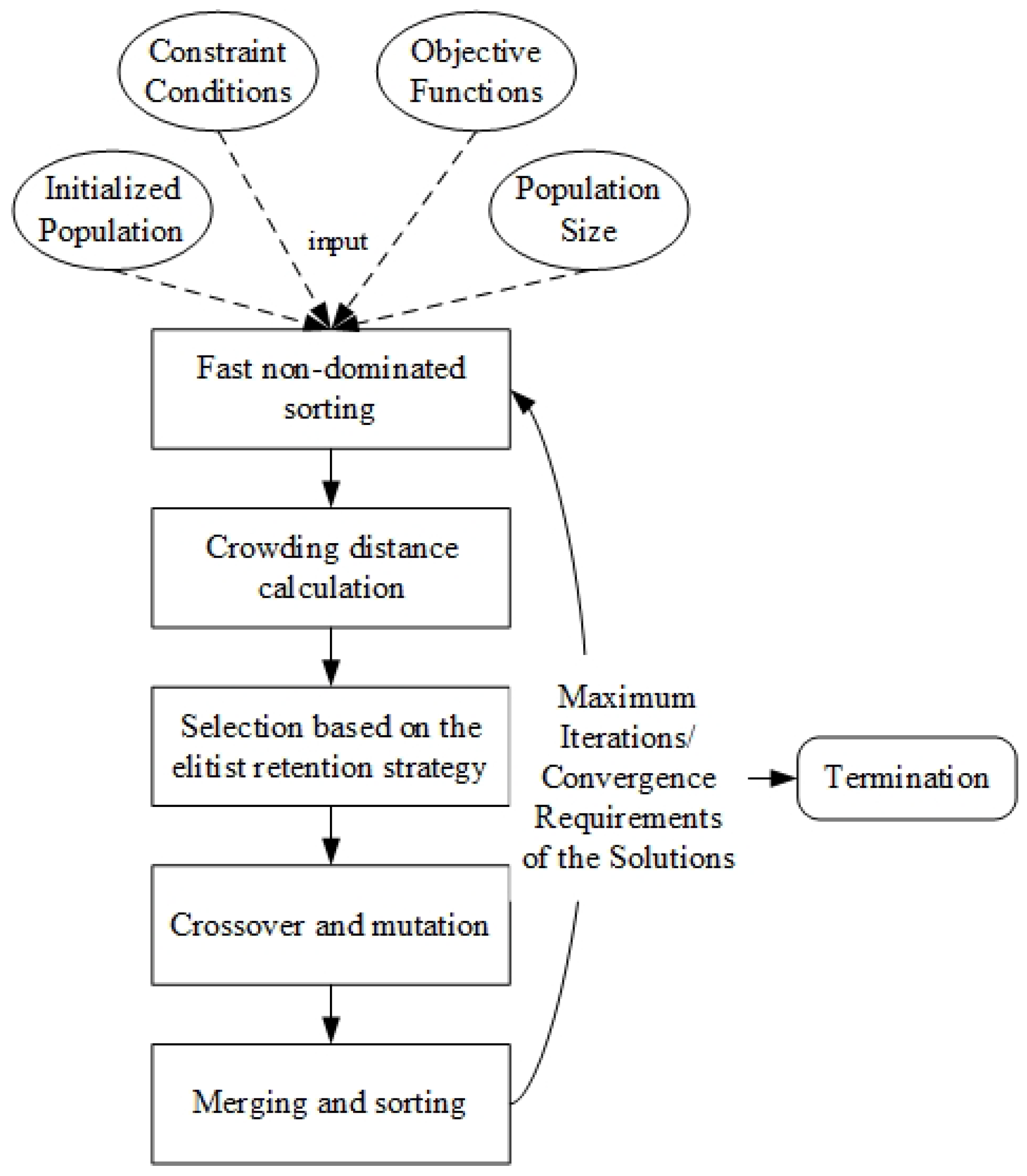
The optimization problem takes the coordinate positions of the basic elements as optimization variables and includes three objective functions and three sets of constraints. In this study, the NSGA-II algorithm is adopted for solution. The NSGA-II algorithm was proposed by Deb et al. [47,48], with the Pareto-front solution set as the output and relevant parameters such as the initialized population, constraint conditions, objective functions, and population size as the inputs. The core process is shown in Figure 1.

First, fast, non-dominated sorting is performed, with the fitness values of each point in the population under multiple objective functions used as the basis for non-dominated sorting, dividing the population into several fronts. The second step is to calculate the crowding distance of each point within each front. The larger the crowding distance is, the greater the contribution of this point to the diversity of the solution set. Then, based on the elitist retention strategy, the points in the non-dominated fronts are selected, and the solutions in the fronts with higher rankings are preferentially selected. When the number of points in the same front exceeds the population size, the points with larger crowding distances are preferentially selected. Next, crossover and mutation operations are performed on the selected parent points to generate new offspring points. Then, the parent generation and the offspring generation are merged, followed by non-dominated sorting, crowding distance calculation, and another round of selection. The first N individuals to enter the next generation are retained. These steps are repeated iteratively until the termination condition is met [47].

2.4. Verification Experiment

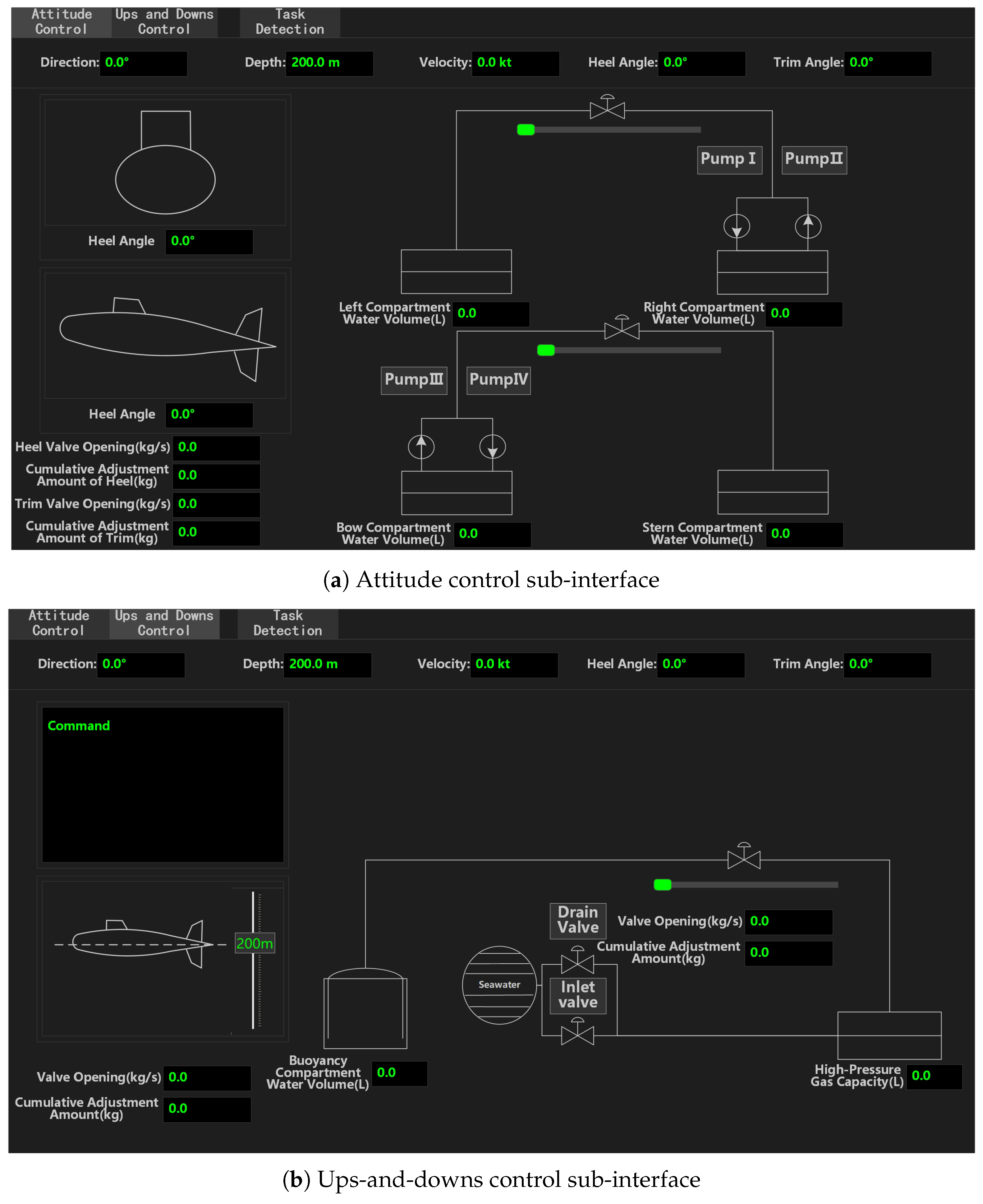
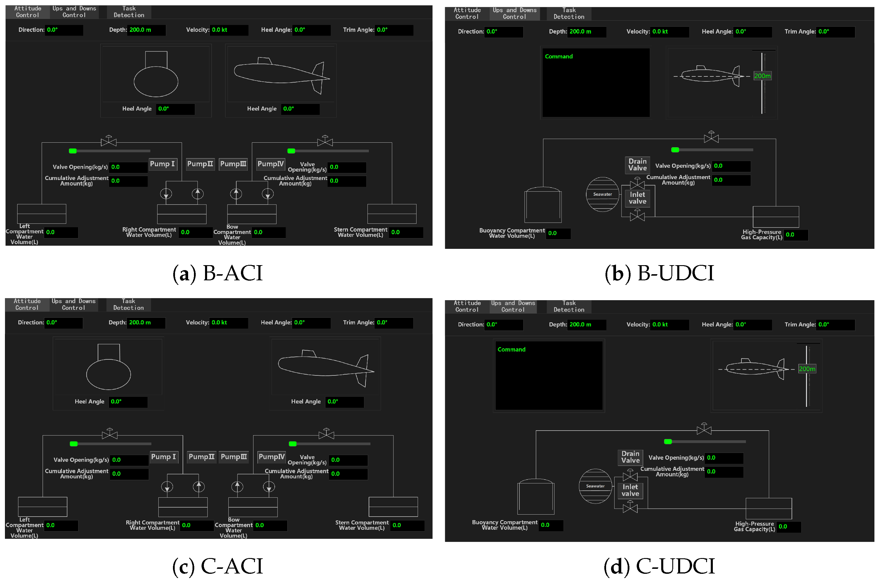
We established a simulation task platform for manned submersibles that abstracts and simplifies the tasks and HMI in real scenarios and complies with the task requirements in real scenarios. The interface of the mechanical support (MS) position in the simulation task platform includes two sub-interfaces: the attitude control interface (ACI) and the ups-and-downs control interface (UDCI). These interfaces can be switched through the menu bar. The original interface is shown in Figure 2.

To determine the minimum sample size that statistically meets the experimental requirements, this study used G*Power 3.1.9 to estimate the sample size and calculated the sample size using repeated-measures ANOVA. The significance level was 0.05, the statistical power was 0.80, the effect value was 0.3, the spherical hypothesis correction coefficient was 1, and the repeated-measures correlation coefficient was 0.5. The pre-statistical power analysis results showed that the minimum required sample size was 15 people. A total of 18 subjects (age: mean = 23.17; SD = ± 1.62) were recruited for this experiment. Due to the fact that operators in the mechanical support positions of manned submersibles were predominantly male, subjects were chosen to be male engineering students with a bachelor’s degree or above; in good health, with normal hearing, with normal vision or corrected vision, without color weakness or color blindness, right-handed, and proficient in operating computers.

The experiment was carried out based on the simulated tasks of the MS position on the submersible simulation platform. The experiment utilized an aSee A3 desktop portable eye tracker to synchronously record eye-movement data.

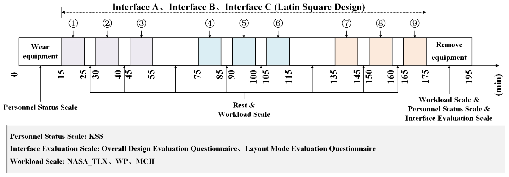
Prior to the experiment, participants underwent one day of training and completed nine experimental tasks in sequence according to the Latin-square sorting results. Each task lasted for 10 min, with a 5 min break after each task and a 20 min break after every three tasks. The sorting of the Latin-square experimental design is shown in Appendix A. After the experiment, the subjects filled out the Overall Design Evaluation Questionnaire and the Layout Mode Evaluation Questionnaire to record their subjective preferences for different interfaces. The evaluation of mental workload adopted the NASA-TLX [49,50]. The subjects were required to fill it out after each simulated task to record their subjective feelings about the workload [51]. This study was approved by the Institutional Review Board (IRB) of Beihang University (BM20240178). The experimental procedure is shown in Figure 3.

IBM SPSS Version 27 was used for the statistical analysis of the experimental data. Due to the small sample size of this experiment, the Shapiro–Wilk test was employed to conduct a normality testing on the data. If $p\ge 0.05$, the data are considered to basically satisfy the normal distribution. Repeated-measures analysis of variance was used to test whether the differences under different layout interfaces were statistically significant.

3. Results

3.1. Task Sequence and Element Usage Sequence

According to the original interface, a total of 24 basic elements are divided. The division results and element numbers are shown in

Table 2. Basic elements of MS-HMIs.

No.	Element	Sub-Interface
$e_1$	Menu bar	ACI/UDCI
$e_2$	Information bar	ACI/UDCI
$e_3$	Heel angle	ACI
$e_4$	Heel-structure diagram	ACI
$e_5$	Heel-pump button	ACI
$e_6$	Heel valve	ACI
$e_7$	Heel-valve opening	ACI
$e_8$	Heel water adjustment volume	ACI
$e_9$	Heel-compartment water volume	ACI
$e_{10}$	Trim angle	ACI
$e_{11}$	Trim-structure diagram	ACI
$e_{12}$	Trim-pump button	ACI
$e_{13}$	Trim valve	ACI
$e_{14}$	Trim-valve opening	ACI
$e_{15}$	Trim adjustment water volume	ACI
$e_{16}$	Trim-compartment water volume	ACI
$e_{17}$	Instruction	UDCI
$e_{18}$	Depth	UDCI
$e_{19}$	Depth-structure diagram	UDCI
$e_{20}$	Depth-pump button	UDCI
$e_{21}$	Depth valve	UDCI
$e_{22}$	Depth-valve opening	UDCI
$e_{23}$	Depth water adjustment	UDCI
$e_{24}$	Depth-compartment water volume	UDCI

.

Based on the task operation specifications, a HTA is conducted on the five typical tasks, and each typical task is decomposed into third-level subtasks. Then, the hierarchical structure of each typical task, the corresponding specific task operations, and interface elements are obtained. The HTA analysis results are shown in Appendix B.

According to the triggering situations of various typical tasks, the trigger counts of the five typical tasks are 1:1:1:5:2, which are respectively denoted as $f_i$, where $i=1-5$. The task sequence and the element usage sequence can be expressed by Equation (19).

$$\left\{\begin{array}{c}T=\left\{(T_1,f_1),(T_2,f_2),(T_3,f_3),(T_4,f_4),(T_5,f_5)\right\}\\ S=\left\{(S_1,f_1),(S_2,f_2),(S_3,f_3),(S_4,f_4),(S_5,f_5)\right\}\end{array}\right.$$

(19)

3.2. Task-Information Network Analysis

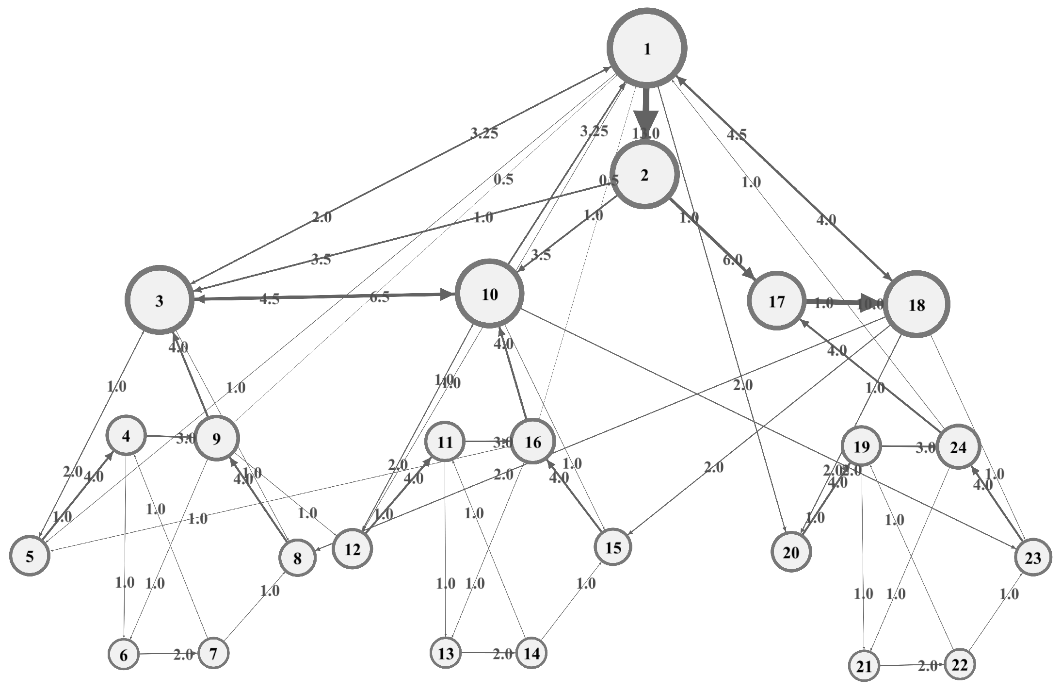
The node set of the Space-P network model contains 24 basic elements, and the adjacency matrix ($A_{24\times 24}$) contains 105 edges. To illustrate the network construction process, consider the first secondary subtask of the heel-angle adjustment task (Check the heel-angle status), which has an element usage sequence of $e_1\to e_2\to e_3$ and a task-trigger frequency of $f_1$ = 1. In the Space-P network, all elements appearing within the same secondary subtask are treated as co-occurring, regardless of their relative order. For the sequence expressed as $e_1\to e_2\to e_3$, three co-occurring pairs are identified: ($e_1$, $e_2$), ($e_1$, $e_3$), and ($e_2$, $e_3$). In accordance with Equation (3), each pair receives a weight contribution of $f_1\times C(e_i,e_j)=1\times 1=1$. The weight of each corresponding edge in the adjacency matrix is increased by this amount. Contributions from all secondary subtasks across all typical tasks are accumulated in this manner to produce the final weighted symmetric adjacency matrix of the Space-P network.

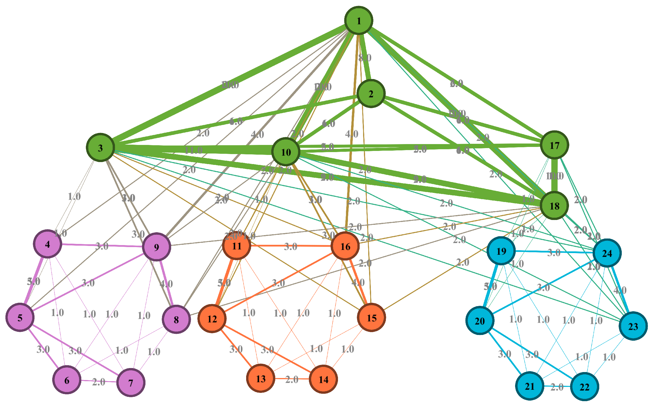
A network model is constructed according to this matrix, using Gephi (version 0.10.1) for visualization, as shown in Figure 4. The thickness of the edges in the figure is proportional to the weight, which intuitively reflects the correlation strength between the basic elements.

In this study, Newman’s fast algorithm was used to conduct a community structure analysis of the Space-P network, with the resolution set to 1.0. A total of 24 nodes were divided into four communities, and the modularity was 0.337. The modularity remained unchanged after adjusting the resolution, indicating that the community structure of this network has high uniformity and stability [52,53]. To verify the reliability of the four-community partition, multiple robustness tests were supplemented. First, the Louvain algorithm yielded Q = 0.425 with identical community division, eliminating the risk of algorithm-specific artifacts. Second, resolution sensitivity analysis with $\gamma$ ranging from 0.5 to 1.2 demonstrated stable four-group segmentation within $\gamma \in [0.8,1.2]$. The elements in Community 1 include $e_1,e_2,e_3,e_{10},e_{17},e_{18}$. The menu bar ($e_1$) and the information bar ($e_2$) are common elements of the two sub-interfaces. Therefore, they need to be divided into two groups, with the remaining communities divided into groups based on sub-interface elements. The basic elements within other communities are all in the same sub-interface. The final grouping results are shown in

Table 3. Basic element grouping based on the Space-P network.

Group	Sub-Interface	Basic Elements
1	ACI	$e_1,e_2,e_3,e_{10}$
2	UDCI	$e_1,e_2,e_{17},e_{18}$
3	ACI	$e_4,e_5,e_6,e_7,e_8,e_9$
4	ACI	$e_{11},e_{12},e_{13},e_{14},e_{15},e_{16}$
5	UDCI	$e_{19},e_{20},e_{21},e_{22},e_{23},e_{24}$

.

The node set of the Space-L network model contains 24 basic elements, and the adjacency matrix ($A_{24\times 24}$) contains 61 directed edges. To illustrate the network construction process, consider the first secondary subtask of the heel-angle adjustment task (Check the heel angle status), which has an element usage sequence of $e_1\to e_2\to e_3$ and a task-trigger frequency of $f_1$ = 1. In the Space-L network, only consecutive transitions between elements are connected, and the direction of each edge reflects the operational order in the task sequence. For the sequence expressed as $e_1\to e_2\to e_3$, two directed edges are generated. In accordance with Equation (4), the directed edge from $e_1$ to $e_2$ receives a weight contribution of $f_1\times 1=1$, and the directed edge from $e_2$ to $e_3$ receives a weight contribution of $f_1\times 1=1$. No edge is generated between $e_1$ and $e_3$, as they are not consecutive in the sequence. This distinguishes the Space-L network from the Space-P network: Space-P captures all pairwise co-occurrences within a subtask, emphasizing the density of element associations, whereas Space-L captures only sequential transitions, emphasizing the logical order of operations.

A network model is constructed according to this matrix and visualized using Gephi (version 0.10.1), as shown in Figure 5. The size of the nodes in the figure is proportional to the weighted degree, which intuitively reflects the usage frequency of the interface elements; the thickness of the edges is proportional to the weight, which intuitively reflects the correlation strength between the basic elements.

Based on the Space-L network, three indicators—namely, weighted DC, BC, and EC—are calculated, among which, $w_{DC}=0.49$, $w_{BC}=0.25$, and $w_{EC}=0.26$. The calculation results of the importance after normalization are shown in

Table 4. Basic element importance based on the Space-L network.

Element	DC	BC	EC	Importance
$e_1$	1.00	1.00	0.86	0.96
$e_2$	0.78	0.06	0.90	0.63
$e_3$	0.77	0.32	1.00	0.72
$e_4$	0.19	0.32	0.22	0.23
$e_5$	0.19	0.31	0.67	0.34
$e_6$	0.00	0.08	0.14	0.05
$e_7$	0.00	0.08	0.05	0.03
$e_8$	0.13	0.21	0.47	0.23
$e_9$	0.30	0.50	0.21	0.32
$e_{10}$	0.77	0.47	0.79	0.70
$e_{11}$	0.19	0.33	0.20	0.23
$e_{12}$	0.19	0.37	0.61	0.34
$e_{13}$	0.00	0.08	0.13	0.05
$e_{14}$	0.00	0.08	0.05	0.03
$e_{15}$	0.13	0.20	0.40	0.22
$e_{16}$	0.30	0.48	0.19	0.31
$e_{17}$	0.56	0.00	0.47	0.40
$e_{18}$	0.73	0.41	0.53	0.60
$e_{19}$	0.19	0.29	0.16	0.21
$e_{20}$	0.19	0.34	0.46	0.30
$e_{21}$	0.00	0.09	0.11	0.05
$e_{22}$	0.00	0.09	0.04	0.03
$e_{23}$	0.13	0.23	0.40	0.22
$e_{24}$	0.28	0.42	0.17	0.29

.

3.3. Layout Optimization Solution Set

The resolution of the simulation interface is 1920 × 1080 pixels. The origin of the coordinate system is located at the top-left corner of the interface, with the x-axis extending horizontally to the right and the y-axis extending vertically downward. The center point is defined as (960, 0). The minimum horizontal spacing between any two interface elements is set to 30 pixels and the minimum vertical spacing is to 10 pixels based on the layout constraints of the simulation platform.

The objects of optimization are the position coordinates of all basic elements. Therefore, the optimization variables include 24 groups of position coordinates. Since there are fixed relative-position relationships between some elements, the position coordinates of one element can be represented by the position coordinates of another element plus the corresponding offset value. After simplification, the final number of optimization variables is reduced to 15 groups of position coordinates.

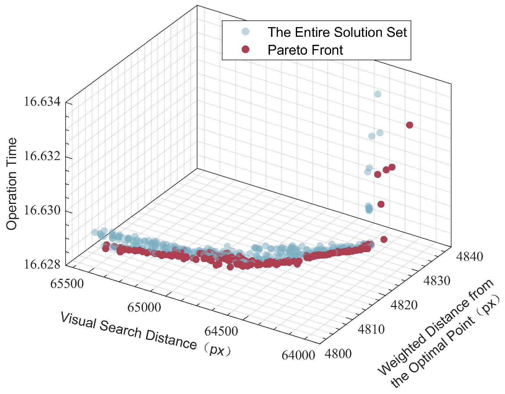
The NSGA-II algorithm is adopted for solution, with the optimization implemented using MATLAB’s (R2024a) gamultiobj solver with the following parameter settings: population size = 500, Pareto fraction = 0.35, crossover operator = crossoverheuristic, crossover fraction = 0.5, mutation operator = mutationadaptfeasible, and maximum generations = 500. All decision variables were treated as integers corresponding to the pixel coordinates of interface-element positions. The initial population was seeded using the original layout, and the algorithm terminated at generation 276 when the spread of the Pareto front fell below the default function tolerance. The solution set is shown in Figure 6.

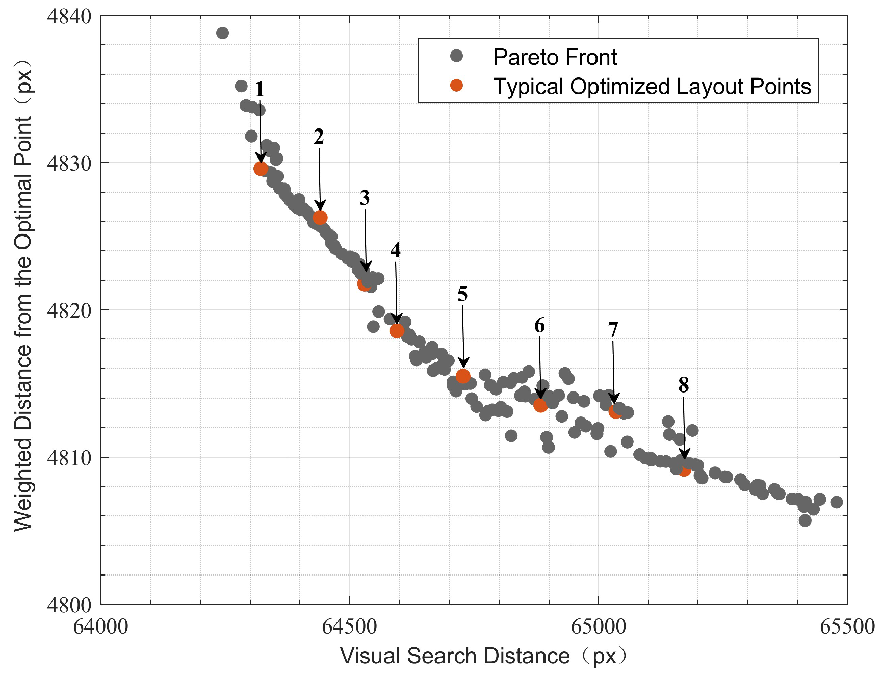
Since the Pareto-front solution set has a small difference in terms of operation time and is concentrated around 16.628, the final layout optimization point is selected near this value. The projected Pareto-front solution set is shown in Figure 7. Its distribution indicates that there is a competitive relationship between the two objective functions—namely, the visual search distance and the weighted distance from the optimal point. Eight typical points are selected from the Pareto front and compared with other points. The difference only lies in the fine adjustment of the positions of a few basic elements (the coordinate change is within 20 px). Therefore, these eight typical points can represent all the layout methods obtained from the model calculation.

When designingthe interface layout, in addition to the constraints, other constraints should also be considered. Based on operating habits, if information elements such as valve opening and water adjustment volume are located near the corresponding valve-control sliders, they should be kept horizontally or vertically aligned with them, thereby excluding typical points 3, 6, 7, and 8. Considering the consistency between sub-interfaces, the functions of heel and trim angles in the ACI are similar to depth and commands in the UDCI. Therefore, the position coordinates should be kept as consistent as possible between the two sub-interfaces. In addition, layouts for the ACI of typical points 2 and 5, as well as typical points 1 and 4, are similar, and layouts for the UDCI of typical points 1 and 2, as well as typical points 4 and 5, are similar.

Therefore, typical points 2 and 4 are selected to form two layouts for the ACI and two layouts for the UDCI. The difference in the ACI mainly lies in whether the positions of e3 and e10 are adjacent, and the difference in the UDCI mainly lies in whether the positions of e17 and e18 are adjacent. The original interface is denoted as A (Figure 1), the interface of typical point 2 is denoted as B, and the interface of typical point 4 is denoted as C, as shown in Figure 8. The values of their objective functions are shown in

Table 5. Objective function of typical optimized layout points 2 and 4.

Typical Point	Operational Duration	Visual Search Distance (px)	Weighted Distance from the Optimal Point (px)
2	16.628	64427.475	4825.922
4	16.628	64624.034	4818.009

.

3.4. Experimental Verification Results

The Shapiro–Wilk test was used to assess the normality of the data for each dependent variable. Results indicated that all variables satisfied the normality assumption ($p\ge 0.05$). Therefore, repeated-measures ANOVA was applied for all subsequent analyses. The descriptive statistical results obtained with respect to the operational performance, eye movement, and subjective evaluations are shown in

Table 6. Descriptive statistical results of the experimental indicators (Mean ± SD).

Experimental Indicators		Interface Layout
		A (Original)	B (Optimized)	C (Optimized)
Operational Performance	Accuracy Rate (%)	85.632 ± 18.062	89.704 ± 17.905	90.135 ± 17.245
	Uncompleted Rate (%)	1.631 ± 3.869	0.284 ± 1.317	0.446 ± 2.135
	Operational Duration (s)	17.594 ± 3.209	16.150 ± 2.666	16.056 ± 2.356
	Completion Duration (s)	21.320 ± 3.543	19.922 ± 2.643	19.617 ± 2.641
Eye Movement	Average Saccade Amplitude (px)	491.552 ± 100.600	407.761 ± 87.579	436.128 ± 74.728
	Average Saccade Speed (px/ms)	5.079 ± 0.483	4.828 ± 0.590	4.810 ± 0.437
Subjective Evaluation	NASA_TXL	7.059 ± 3.661	6.612 ± 3.692	6.329 ± 3.041
	Evaluation of Overall Design	3.280 ± 0.781	4.267 ± 0.488	4.480 ± 0.506
	Evaluation of Layout Mode	3.233 ± 0.644	4.392 ± 0.425	4.458 ± 0.374

. The repeated-measures ANOVA results of the interface layout are shown in

Table 7. Repeated-measures ANOVA results of the interface layout. (* $p\le 0.05$, ** $p\le 0.01$, and *** $p\le 0.001$).

Experimental Indicators		Mauchly’s Test		Repeated-Measures ANOVA
		W	p	F	p	Partial ${\mathsf{\eta }}^{\mathbf{2}}$
Operational Performance	Accuracy Rate (%)	0.990	0.948	1.831	0.180	0.123
	Uncompleted Rate (%)	0.803	0.300	3.939	0.033 *	0.247
	Operational Duration (s)	0.865	0.450	5.333	0.012 *	0.308
	Completion Duration (s)	0.925	0.650	6.725	0.005 **	0.359
Eye Movement	Average Saccade Amplitude (px)	0.195	<0.001	5.970	0.025 *	0.315
	Average Saccade Speed (px/ms)	0.364	0.002	12.643	0.002 **	0.493
Subjective Evaluation	NASA_TXL	0.810	0.186	0.320	0.729	0.018
	Evaluation of Overall Design	0.578	0.012	38.177	<0.001 ***	0.692
	Evaluation of Layout Mode	0.928	0.551	63.405	<0.001 ***	0.789
Experimental Indicators		Correction		Paired Comparison (p)
				A-B	A-C	B-C
Operational Performance	Accuracy Rate (%)	—		0.068	0.145	0.968
	Uncompleted Rate (%)	—		0.053	0.028 *	0.721
	Operational Duration (s)	—		0.036 *	0.010 *	0.866
	Completion Duration (s)	—		0.030 *	0.004 **	0.427
Eye Movement	Average Saccade Amplitude (px)	0.554		0.019 *	0.044 *	0.115
	Average Saccade Speed (px/ms)	0.611		0.004 **	0.002 **	0.571
Subjective Evaluation	NASA_TXL	—		0.449	0.569	0.994
	Evaluation of Overall Design	0.703		<0.001 ***	<0.001 ***	<0.001 ***
	Evaluation of Layout Mode	—		<0.001 ***	<0.001 ***	<0.001 ***

.

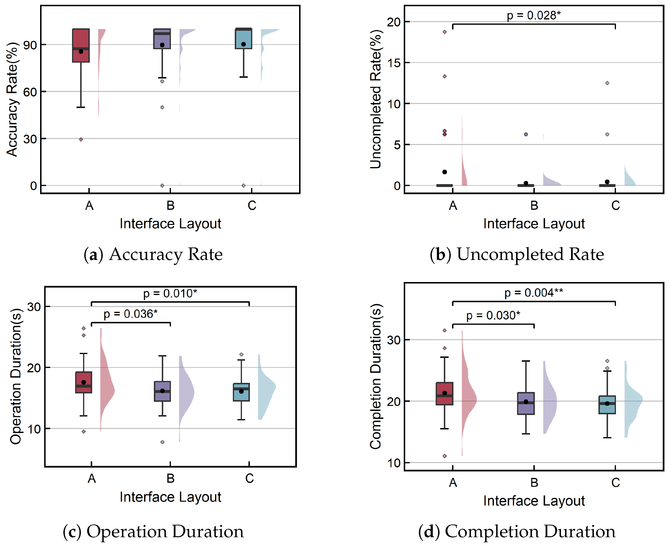
Compared with the original interface (A), both the layout-optimized interfaces (B and C) significantly improved operational performance, and interface C is more effective. As shown in Figure 9a, the accuracy rates of interfaces B and C increased. As shown in Figure 9b, the average uncompleted rate of interface C significantly decreased by 1.2% (p = 0.028). As shown in Figure 9c, the operational duration of interface B was significantly shortened by 1.4 s, corresponding to a reduction of approximately 8.2% (p = 0.036), and that of interface C was significantly shortened by 1.5 s, corresponding to a reduction of approximately 8.7% (p = 0.010). As shown in Figure 9d, the completion duration of interface B was significantly shortened by 1.4 s, corresponding to a reduction of approximately 6.5% (p = 0.030), and that of interface C was significantly shortened by 1.5 s, corresponding to a reduction of approximately 7.9% (p = 0.004).

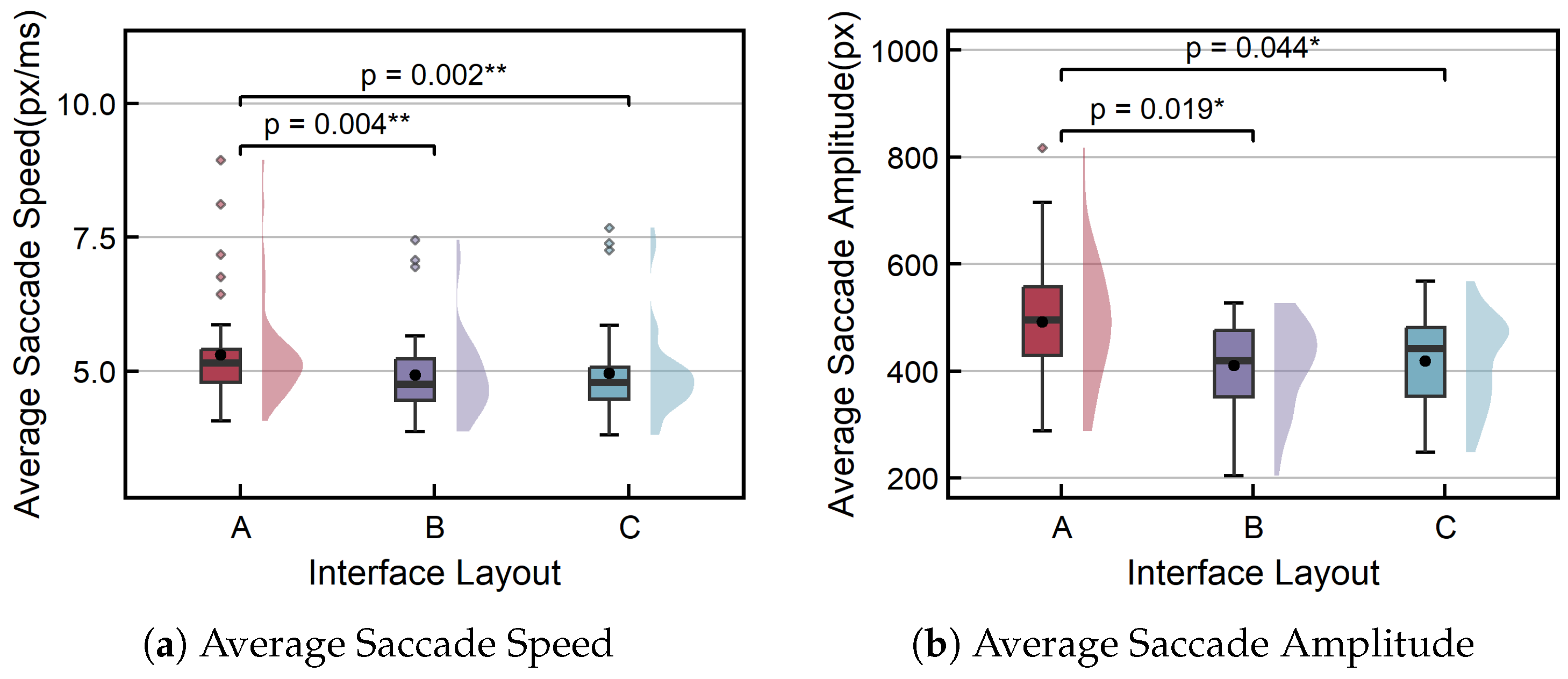
When using the two layout-optimized interfaces, both the average saccade speed and the average saccade amplitude were significantly decreased. As shown in Figure 10a, the average saccade speed of interface B was decreased by 17.1% (p = 0.004), and that of interface C was decreased by 11.2% (p = 0.002). As shown in Figure 10b, the average saccade amplitude of interface B was decreased by 4.9% (p = 0.019), and that of interface C was decreased by 5.3% (p = 0.044).

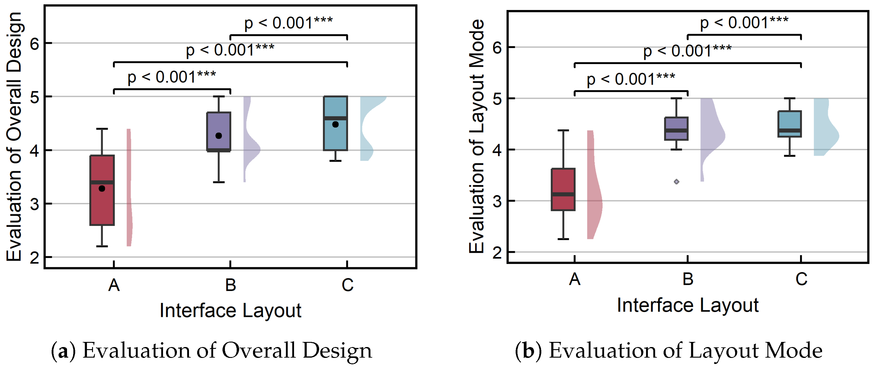
The NASA_TXL scale is used to measure the mental workload. The average mental workload of the optimized interfaces is slightly lower, but there is no significant difference between different layouts. The overall design evaluation questionnaire and the layout-mode evaluation questionnaire record the subjective evaluations of the subjects on the three interface layouts. As shown in Figure 11a, in the evaluation of the overall design, the scores of both interface B and interface C are significantly higher than those of the original interface (A). From the perspective of the score distribution, more subjects think that the layout-optimized interface (C) is better. As shown in Figure 11b, in the evaluation of the layout mode, the scores of both interface B and interface C are significantly higher than those of the original interface (A).

This study compared performance under different interface layouts along three dimensions: operational performance, eye movement, and subjective evaluation. The experimental results show that both interface B and interface C are significantly superior to the original interface in terms of operational performance and subjective scores for the design of the interface, verifying the effectiveness of the layout optimization. In addition, compared with interface B, interface C performs better on multiple indicators. Therefore, interface C is selected as the optimized layout result for MS-HMIs.

4. Discussion

This paper proposes an approach for optimizing the layout of MS-HMIs in manned submersibles, with the goal of improving operator safety and work efficiency. By comprehensively considering operator characteristics, task complexity, and interface-element factors, the proposed method enhances both usability and user experience. Given the complex and varied information and diverse operational tasks in MS-HMIs, our approach leverages complex network theory for layout optimization. Compared with existing methods, it offers broad applicability in practical settings, enabling the interface to adapt more effectively to operational changes and challenges, thereby improving operator efficiency and satisfaction [8,9,10,11,54].

The use of Space-P and Space-L networks for the grouping and evaluation of the importance of basic elements enables us to more effectively identify and classify key functional elements in MS-HMIs. Compared with traditional interface design methods, the Space-P network provides a structured way to understand requirements and more clearly identify which elements are most suitable for combination, while the Space-L network further clarifies the importance of each element in personnel operations through correlation analysis of these basic elements [27,28]. The combination of these methods not only makes our optimization method more targeted but also effectively reduces the cognitive load that may be encountered during the operation process.

In practice, this complex network-based optimization method demonstrates clear advantages, producing an interface design that better aligns with real-world needs. Compared with traditional single-objective methods, the multi-objective optimization strategy considers multiple design dimensions, including operator habits, element importance, and visual search efficiency. By applying advanced multi-objective optimization techniques, such as the genetic algorithm, operator performance can be enhanced while maintaining interface functionality. This comprehensive approach yields more balanced optimization results, significantly improves interface adaptability across different operational positions [55,56,57], and provides a foundation for future research in submersible design, highlighting the method’s broad application potential.

In addition, there are still some aspects that warrant further exploration. Regarding the participant sample, engineering students were used as proxies for professional submersible operators. Although all participants completed training to ensure basic task proficiency, this cannot fully replicate the domain expertise, operational experience, and stress-response patterns characteristic of trained submersible crews. According to a survey of the actual MS operator population in the manned submersible program under study, the operational crew is exclusively male and predominantly in the young-adult age range, which is consistent with the demographic profile of our participant sample. Nevertheless, the use of student participants limits the generalizability of the findings to real operational contexts. Future studies are recommended to recruit professional submersible operators and conduct validation experiments under higher-fidelity operational scenarios to further confirm the effectiveness of the proposed layout optimization method. When constructing a task–information network using the Space-P and Space-L methods, the complex interdependencies among interface elements may not be fully captured. Future research could explore advanced or emerging network modeling approaches to more comprehensively represent these relationships and enable deeper analysis. In developing the multi-objective optimization model, the interface elements were simplified as fixed-size rectangles to reduce computational complexity. However, in practical applications, interface elements may have irregular shapes or variable sizes. Future studies could incorporate shape diversity and size adaptability to achieve a more flexible and realistic layout optimization scheme. Additionally, the transfer of optimized layouts to real submersible systems involves practical engineering constraints not considered in the present study, such as hardware limitations and system integration requirements, which would require additional validation. Finally, although the proposed method was developed in the context of a manned submersible HMI, its underlying framework is not inherently domain-specific and is potentially applicable to other maritime HMIs, nuclear control rooms, aircraft cockpits, and other safety-critical display systems, representing a promising direction for future research.

5. Conclusions

Operators of submersibles are required to continuously monitor large volumes of real-time information on the HMI to ensure stable system operation. Optimizing the HMI layout is critical to enhancing operator efficiency, reducing cognitive workload, and minimizing potential safety risks. This study proposes a systematic and task-driven method for optimizing submersible HMI layouts. Based on ergonomic design principles, the task sequences and element usage sequences of typical operations were analyzed using the HTA approach, and a task-information network for the HMI was constructed. The grouping and importance of basic interface elements were determined through analysis of the network topology. The layout optimization problem was formulated as a multi-objective optimization task solved using the NSGA-II algorithm. As a case study, the mechanical support position interface was analyzed, resulting in two optimized layout designs. Experimental verification showed that the optimized interfaces significantly improved operator performance, eye-movement efficiency, and subjective evaluations, demonstrating the effectiveness of the proposed layout optimization method. It should be noted that the experimental validation is preliminary and based on a simulated environment with a small sample of non-professional participants, and further validation with trained submersible operators, larger participant samples, and more realistic operational scenarios is necessary before the method can be recommended for direct application in real manned submersible design.

References

1. Hunter, A.; Hazen, M.; Randall, T. VICTORIA Class Submarine Human-in-the-Loop Experimentation Plan; Defence Research Development Canada: Ottawa, ON, Canada, 2014.
2. Shin, G.H.; Song, C.U.; Kim, D. Quantitative Assessment of Vessel Traffic Service Center Workload: Development and Validation of the Vessel Traffic Service Operator Workload Index (VOWI). J. Mar. Sci. Eng. 2025, 13, 299. [Google Scholar] [CrossRef] [Scilit]
3. Li, Z.; Daxin, Y.; Yiqun, W. The Effect of Information Display on Human Reliability in a Digital Control Room. China Saf. Sci. J. 2010, 20, 81. [Google Scholar]
4. Yang, C.; Pang, L.; Zhao, B.; Wu, W.; Cao, X. Experimental investigation of submersible buoyancy regulation and support task performance under different levels of automation and varying workloads. Int. J. Ind. Ergon. 2025, 106, 103713. [Google Scholar] [CrossRef] [Scilit]
5. Wästlund, E.; Norlander, T.; Archer, T. The effect of page layout on mental workload: A dual-task experiment. Comput. Hum. Behav. 2008, 24, 1229–1245. [Google Scholar] [CrossRef] [Scilit]
6. Simonin, J.; Kieffer, S.; Carbonell, N. Effects of Display Layout on Gaze Activity During Visual Search. In Human-Computer Interaction—INTERACT 2005; Costabile, M.F., Paternò, F., Eds.; Lecture Notes in Computer Science; Springer: Berlin/Heidelberg, Germany, 2005; Volume 3585, pp. 1054–1057. [Google Scholar] [CrossRef] [Scilit]
7. Zhou, Y.; Chen, D.; Xiao, J.; Wang, H. An evaluation method for HMI of deep-sea manned submersible based on human reliability. Sci. Rep. 2023, 13, 14507. [Google Scholar] [CrossRef] [Scilit] [PubMed]
8. Bartlett, M.W.; Smith, L.A. Design of Control and Display Panels Using Computer Algorithms. Hum. Factors J. Hum. Factors Ergon. Soc. 1973, 15, 1–7. [Google Scholar] [CrossRef] [Scilit]
9. Bonney, M.C.; Williams, R.W. CAPABLE. A Computer Program to Layout Controls and Panels. Ergonomics 1977, 20, 297–316. [Google Scholar] [CrossRef] [Scilit]
10. Banks, W.W.; Boone, M.P. A Method for Quantifying Control Accessibility. Hum. Factors J. Hum. Factors Ergon. Soc. 1981, 23, 299–303. [Google Scholar] [CrossRef] [Scilit]
11. Pulat, B.M.; Ayoub, M.A. A Computer-Aided Panel Layout Procedure for Process Control Jobs—LAYGEN. IIE Trans. 1985, 17, 84–93. [Google Scholar] [CrossRef] [Scilit]
12. Ying, Q.; Zhongxiang, Z.; En-rong, M.; Zhenghe, S.; Weibin, H.; XianXue, Z. Study on priorities of human-machine interface in combine harvester cab. Trans. Chin. Soc. Agric. Mach. 2009, 40, 43–47. [Google Scholar]
13. Wang, M.J.; Liu, C.M.; Pan, Y.S. Computer-aided panel layout using a multi-criteria heuristic algorithm. Int. J. Prod. Res. 1991, 29, 1215–1233. [Google Scholar] [CrossRef] [Scilit]
14. Şenol, M.B.; Dağdeviren, M.; Çilingir, C.; Kurt, M. Display panel design of a general utility helicopter by applying quantitative and qualitative approaches. Hum. Factors Ergon. Manuf. Serv. Ind. 2010, 20, 73–86. [Google Scholar] [CrossRef] [Scilit]
15. Wang, Y.-K.; Ren, J.-J.; Li, A.-F.; Meng, H.-N. Layout optimization design of operation interface in mining excavator cab. Chin. J. Eng. Des. 2020, 27, 469–477. [Google Scholar] [CrossRef]
16. Meng, X.; Sun, H.; Kang, J. Equipment Layout Optimization Based on Human Reliability Analysis of Cabin Environment. J. Mar. Sci. Eng. 2021, 9, 1263. [Google Scholar] [CrossRef] [Scilit]
17. Fay, D.; Stanton, N.A.; Roberts, A. Designing New Interfaces for Submarines: From Cognitive Work Analysis to Ecological Interface Design. In Proceedings of the Advances in Human Aspects of Transportation; Stanton, N.A., Landry, S., Di Bucchianico, G., Vallicelli, A., Eds.; Springer: Cham, Switzerland, 2017; pp. 413–425. [Google Scholar] [CrossRef] [Scilit]
18. Yang, C.; Pang, L.; Wu, W.; Cao, X. Human-Machine Function Allocation Method for Submersible Fault Detection Tasks. Mathematics 2024, 12, 3615. [Google Scholar] [CrossRef] [Scilit]
19. Newman, M.E.J. Networks: An introduction; Oxford University Press: Oxford, UK; New York, NY, USA, 2010. [Google Scholar]
20. Stanton, N.A.; Baber, C. Modelling Command and Control: Event Analysis of Systemic Teamwork; CRC Press: London, UK, 2017. [Google Scholar] [CrossRef] [Scilit]
21. Stanton, N.A. Representing distributed cognition in complex systems: How a submarine returns to periscope depth. Ergonomics 2014, 57, 403–418. [Google Scholar] [CrossRef] [Scilit] [PubMed]
22. Duryea, D.M.; Lindstrom, C.E.; Sayegh, R. Submarine imaging systems: Developing improved capabilities and technologies. In Proceedings of the Sensors, and Command, Control, Communications, and Intelligence (C3I) Technologies for Homeland Security and Homeland Defense VII; SPIE: Bellingham, WA, USA, 2008; Volume 6943, pp. 256–263. [Google Scholar] [CrossRef] [Scilit]
23. Stanton, N.A.; Roberts, A.P.J. Examining Social, Information, and Task Networks in Submarine Command and Control. IEEE Trans. Hum.-Mach. Syst. 2018, 48, 252–265. [Google Scholar] [CrossRef] [Scilit]
24. Zheng, D. Research on Topological Structure of Human-Computer Interactive Information Network in Complex Task Environment. Master’s Thesis, Southeast University, Nanjing, China, 2019. [Google Scholar]
25. Wang, W. Key Technologies of Aircraft Cockpit’s Ergonomic Design and Comprehensive Evaluation. Ph.D. Thesis, Northwestern Polytechnical University, Xi’an, China, 2017. [Google Scholar]
26. Wang, W.; Yu, S.; Fan, W.; Deng, L. Research and Application of the Community Structure in the Display and Control Devices of Cockpit. Mach. Des. Manuf. 2015, 7, 227–230. [Google Scholar]
27. Wu, H.; Wang, H.Y.; Chen, X.J.; Xue, C.Q. Research on Layout Design of Situation Interface Based on Comprehensive Importance Evaluation of Nodes. In Proceedings of the 2020 IEEE International Conference on Industrial Engineering and Engineering Management (IEEM); IEEE: New York, NY, USA, 2020; pp. 562–566. [Google Scholar] [CrossRef] [Scilit]
28. Wang, H.; Yu, S.; Chen, D.; Zhang, W.; Chen, C. Mission-oriented human-machine interaction information importance assessment of deep-sea manned submersible. Comput. Integr. Manuf. Syst. CIMS 2024, 30, 1683–1693. [Google Scholar] [CrossRef]
29. Yang, C.; Pang, L.; Cao, X.; Xue, P.; Zhao, B.; Wu, W. Impact of Automation Levels in Different Information Processing Stages on Submersible Mechanical Support Operational Work Performance Under Unbalanced Workloads. Int. J. Hum.–Comput. Interact. 2025, 42, 357–373. [Google Scholar] [CrossRef] [Scilit]
30. Sanders, M.S. Human Factors in Engineering and Design; McGraw-Hill: New York, NY, USA, 1993. [Google Scholar]
31. Cooper, A.; Reimann, R.; Cronin, D.; Noessel, C. About Face: The Essentials of Interaction Design, 4th ed.; Wiley Publishing: Hoboken, NJ, USA, 2014. [Google Scholar]
32. Wang, L.-G.; Yuan, X.-G. Computer Aided Design of Control Panels Based on Ergonomics. Acta Aeronaut. Astronaut. Sin. 1999, 20, 46–47. [Google Scholar]
33. Margaritis, S.; Marmaras, N. Supporting the design of office layout meeting ergonomics requirements. Appl. Ergon. 2007, 38, 781–790. [Google Scholar] [CrossRef] [Scilit] [PubMed]
34. Benyon, D. Designing Interactive Systems: A Comprehensive Guide to HCI and Interaction Design; Pearson: Boston, MA, USA, 2013. [Google Scholar]
35. ISO 11064-1:2000 (En); Ergonomic Design of Control Centres. ISO: Geneva, Switzerland, 2000.
36. Diaper, D.; Stanton, N. (Eds.) The Handbook of Task Analysis for Human-Computer Interaction; CRC Press: Boca Raton, FL, USA, 2003. [Google Scholar] [CrossRef] [Scilit]
37. He, D.; Liu, Z.; Wang, B. Complex Systems and Complex Networks; Higher Education Press: Beijing, China, 2009. [Google Scholar]
38. Newman, M.E.J.; Girvan, M. Finding and evaluating community structure in networks. Phys. Rev. E 2004, 69, 026113. [Google Scholar] [CrossRef] [Scilit] [PubMed]
39. Newman, M.E.J. Fast algorithm for detecting community structure in networks. Phys. Rev. E 2004, 69, 066133. [Google Scholar] [CrossRef] [Scilit] [PubMed]
40. Bonacich, P. Factoring and weighting approaches to status scores and clique identification. J. Math. Sociol. 1972, 2, 113–120. [Google Scholar] [CrossRef] [Scilit]
41. Goh, K.I.; Oh, E.; Kahng, B.; Kim, D. Betweenness centrality correlation in social networks. Phys. Rev. E 2003, 67, 017101. [Google Scholar] [CrossRef] [Scilit] [PubMed]
42. Lü, L.; Zhou, T.; Zhang, Q.M.; Stanley, H.E. The H-index of a network node and its relation to degree and coreness. Nat. Commun. 2016, 7, 10168. [Google Scholar] [CrossRef] [Scilit] [PubMed]
43. Anderson, J.R. Cognitive Psychology and Its Implications, 7th ed.; Worth Publishers: New York, NY, USA, 2010. [Google Scholar]
44. Fitts, P.M. The information capacity of the human motor system in controlling the amplitude of movement. J. Exp. Psychol. Gen. 1992, 121, 262–269. [Google Scholar] [CrossRef] [Scilit] [PubMed]
45. Jiang, R.; Gu, Z. Current Theoretical Developments and Applications of Fitts’ Law: A Literature Review. In Proceedings of the Advances in Ergonomics in Design; Rebelo, F., Soares, M.M., Eds.; Springer: Cham, Switzerland, 2020; pp. 753–760. [Google Scholar] [CrossRef] [Scilit]
46. MacKenzie, I.S. Fitts’ law as a research and design tool in human-computer interaction. Hum.-Comput. Interact. 1992, 7, 91–139. [Google Scholar] [CrossRef] [Scilit] [PubMed]
47. Deb, K.; Pratap, A.; Agarwal, S.; Meyarivan, T. A fast and elitist multiobjective genetic algorithm: NSGA-II. IEEE Trans. Evol. Comput. 2002, 6, 182–197. [Google Scholar] [CrossRef] [Scilit]
48. Srinivas, N.; Deb, K. Muiltiobjective Optimization Using Nondominated Sorting in Genetic Algorithms. Evol. Comput. 1994, 2, 221–248. [Google Scholar] [CrossRef] [Scilit]
49. Miller, K.H. Timeline Analysis Program (TLA-1); Technical Report NASA-CR-144942; National Aeronautics and Space Administration (NASA): Washington, DC, USA, 1976.
50. Hart, S.G.; Staveland, L.E. Development of NASA-TLX (Task Load Index): Results of Empirical and Theoretical Research. Adv. Psychol. 1988, 52, 139–183. [Google Scholar] [CrossRef] [Scilit]
51. ISO 9241-11:2018(en); Ergonomics of Human-System Interaction. ISO: Geneva, Switzerland, 2018.
52. Newman, M.E.J. Modularity and community structure in networks. Proc. Natl. Acad. Sci. USA 2006, 103, 8577–8582. [Google Scholar] [CrossRef] [Scilit] [PubMed]
53. Fortunato, S.; Barthélemy, M. Resolution limit in community detection. Proc. Natl. Acad. Sci. USA 2007, 104, 36–41. [Google Scholar] [CrossRef] [Scilit] [PubMed]
54. Jiang, X.; Wang, X.; Wang, B.; Deng, B. Research on Information Interaction Interface Optimization Based on Cognitive Load. In Proceedings of the 2024 4th International Conference on Computational Modeling, Simulation and Data Analysis, Hangzhou, China, 6–8 December 2024; Association for Computing Machinery: New York, NY, USA; pp. 625–633. [Google Scholar] [CrossRef] [Scilit]
55. Oulasvirta, A.; Dayama, N.R.; Shiripour, M.; John, M.; Karrenbauer, A. Combinatorial Optimization of Graphical User Interface Designs. Proc. IEEE 2020, 108, 434–464. [Google Scholar] [CrossRef] [Scilit]
56. Tufano, F.; Bahadure, S.W.; Tufo, M.; Novella, L.; Fiengo, G.; Santini, S. An Optimization Framework for Information Management in Adaptive Automotive Human–Machine Interfaces. Appl. Sci. 2023, 13, 10687. [Google Scholar] [CrossRef] [Scilit]
57. Ma, L.; Chen, D.; Yan, Y.; An, W. An optimization design method for submarine cabins based on intelligent algorithms. Int. J. Nav. Archit. Ocean Eng. 2025, 17, 100642. [Google Scholar] [CrossRef] [Scilit]
Figure 1. Schematic illustration of the optimization process.
Jmse 14 01176 g001
Figure 2. The original interface of the MS position of manned submersibles.
Jmse 14 01176 g002
Figure 3. Experimental procedure.
Jmse 14 01176 g003
Figure 4. Space-P network structure. Nodes represent basic interface elements ( e 1 – e 24 ). Edges represent co-occurrence relationships between elements within the same secondary subtask. Edge thickness is proportional to edge weight, with higher weight indicating more frequent co-occurrence across typical task sequences. Node color indicates community membership, corresponding to the four communities identified through Newman’s fast algorithm (Q = 0.337).
Jmse 14 01176 g004
Figure 5. Space-L network structure. Nodes represent basic interface elements ( e 1 – e 24 ). Directed edges represent sequential transitions between elements in the task operation sequences, with edge direction indicating operational order. Edge thickness is proportional to edge weight, reflecting the frequency of each transition across typical task sequences. Node size is proportional to weighted degree, reflecting the overall usage frequency of each interface element.
Jmse 14 01176 g005
Figure 6. Distributions of the Pareto-front solution set. The three axes represent the three objective functions: F ( 1 ) , weighted distance from the optimal point (px); F ( 2 ) , operation time (s); F ( 3 ) , visual search distance (px). Each point in the solution set represents a feasible layout configuration. The concentration of solutions around F ( 2 ) ≈ 16.628 s indicates that operational duration converges rapidly, while trade-offs between F ( 1 ) and F ( 3 ) remain across the solution set).
Jmse 14 01176 g006
Figure 7. Projection of the Pareto-front solution set (Red dots indicates typical optimized layout points).
Jmse 14 01176 g007
Figure 8. Optimized MS-HMI layout based on the multi-objective optimization results.
Jmse 14 01176 g008
Figure 9. Statistical analysis of operational performance under different interface layouts. (* p ≤ 0.05 , ** p ≤ 0.01 ).
Jmse 14 01176 g009
Figure 10. Statistical analysis of eye-movement metrics under different interface layouts. (* p ≤ 0.05 , ** p ≤ 0.01 ).
Jmse 14 01176 g010
Figure 11. Statistical analysis of subjective evaluation results under different interface layouts (*** p ≤ 0.001 ).
Jmse 14 01176 g011