Impact of Tropical Cyclones on the Variation in Surface Indonesian Throughflow During Boreal Winter

Abstract

In the boreal winter of the Northern Hemisphere, a weakening of the surface Indonesian throughflow (ITF) is commonly observed. The intraseasonal mechanism of the weakening, namely, the impact of the atmospheric Madden–Julian Oscillation (MJO), is well-known and has been extensively studied. However, a significantly low volume transport of ITF (<100 m in depth) was also observed in the Makassar Strait during the traverse of tropical cyclones (TCs). The observed transport decrease is 0.31 Sv (1 Sv = 10⁶ m³/s) on average, which is ~70% of the estimated influence of the MJO. The time scale of the incurred variation is up to 30 days, comparable to the time of 20–90 days caused by the MJO. The winds in the TC circulation have a major impact on the Makassar Strait’s ITF transport reduction. Numerical experiments reveal that the reduction is due to the along-strait sea level anomaly (SLA) variability that is forced by the winds from the upstream region. The mechanism involves the propagation of coastal Kelvin waves along the Sulawesi Sea generated by the TCs and is confirmed by theoretical analysis. Based on the numerical experiments, this mechanism contributes ~40% to the total ITF transport reduction, while the large-scale guiding circulation surrounding the TCs may contribute to the remaining ITF transport reduction. These results support that TCs are also important forcing components in the intraseasonal variation in surface ITF.

1. Introduction

The Indonesian throughflow (ITF) is part of the global ocean circulation that connects the low-latitude Pacific and Indian Oceans. It traverses maritime South Asia and Southeast Asia, where numerous narrow straits and small interior basins make the circulation very complex in this region [1,2]. The interaction between the ITF and large-scale phenomena occurring from intraseasonal to decadal timescales leads to substantial variabilities in the flow [3,4,5,6,7]. However, current understanding is limited by the availability of observations [8,9]. Continuous improvement of our knowledge is necessary so that the role of the flow in global climate variability can be better addressed [2,9,10,11,12,13].

There are two branches of ITF traversing the maritime continent between the Pacific and Indian Oceans [9]. The western branch refers to the flow of Pacific origin that passes through the Sulawesi Sea and Makassar Strait. This branch accounts for approximately 80% of total ITF transport and is the main pathway for the upper-layer (0–700 m) of flow [8]. The eastern branch refers to a much deeper throughflow of the Pacific water (>1500 m), which runs primarily via the Maluku and Lifamala Seas [14].

It is well known that the volume transport of surface ITF in the Makassar Strait is significantly weakened in the boreal winter [8,15]. The weakening is an important phenomenon affecting the flow’s variability [10]. In observations, the weakening is about 6–7 Sv (1 Sv = 10⁶ m³/s) less than the climatological annual mean [8,15,16]. Of this variability, up to 5 Sv is associated with seasonal variation, and 2 Sv is associated with intraseasonal variation [8,17,18,19,20].

Seasonally, the weakening is mainly due to the impact of the Asian–Australian monsoon, which causes local precipitation and runoff from Kalimantan, Indonesia, and forms a freshwater pressure head in the southern Makassar Strait that impedes the southward flow in the strait [8,10,16,21,22,23]. A recent study suggests that the freshwater influence contributes ~70% to the total seasonal variability in the dynamic height gradient along the Makassar Strait [15].

Intraseasonally, atmospheric dynamics, namely, the Madden–Julian Oscillation (MJO), are the key drivers of the ITF variability, with the influence also mainly from the downstream region of the Makassar Strait [8,9,18,19,22,24]. Specifically, there are two ways in which the ITF transport is affected during an MJO event. One is related to the intrusion of Kelvin waves formed in the equatorial Indian Ocean, which propagate along the Java Islands, intrude into the Makassar Strait, or continue to propagate to the Ombai Strait or the Timor Passage and cause a weaker ITF below the thermocline [18,22,24]. The other involves the weakening of surface ITF by local wind anomalies in the Java Sea [18,19]. In the active phases (phases 4–5) of MJOs, the wind stress along the coast of the Java Sea leads to a rise in sea surface height in the southern Makassar Strait, which ultimately results in a weakening of the surface ITF [19].

Despite the primary downstream influences from MJOs, the intraseasonal ITF of the Makassar Strait may be modulated because of the upstream influence from the Sulawesi Sea. Qiu et al. [25] observed a 50-day flow oscillation of the Sulawesi Sea due to the intrusion of resonant Rossby waves, which have a large impact on the throughflow in the Makassar Strait. Based on numerical simulations, Masumoto et al. [26] reported that an intraseasonal variability in ITF transport of approximately 40 days can be induced by eddies generated at the entrance of the Sulawesi Sea between Mindanao and the Halmahera Islands.

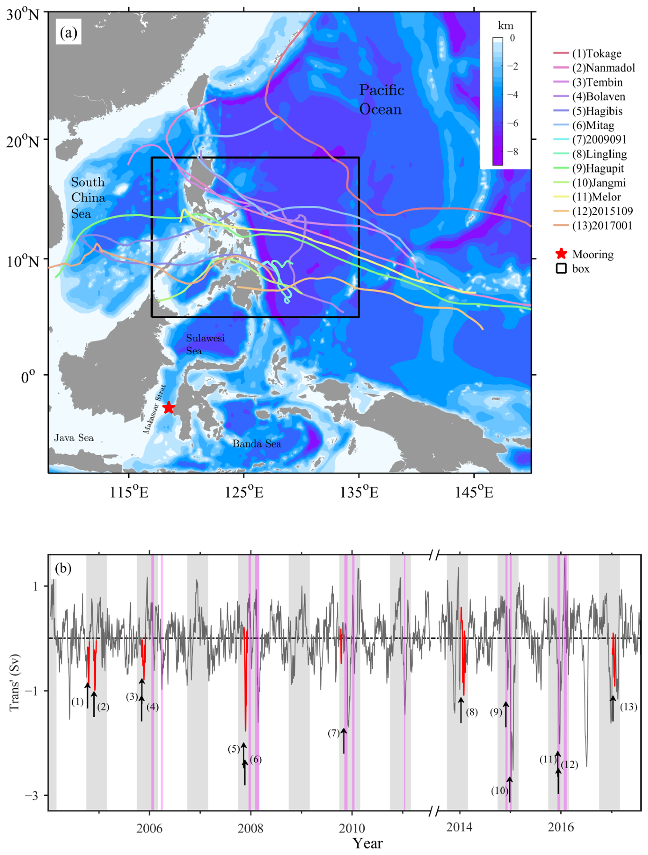
During boreal winter, the formation and pathway of northwest Pacific tropical cyclones (TCs) tend to shift southwestward and increase surface flow variability in the low-latitude Sulawesi Sea [27,28]. Moreover, during the active phases of MJOs, the occurrence of TCs is expected to increase by 10% in winter, which increases the potential to impact the intraseasonal ITF [29,30]. Figure 1b shows the observed subseasonal variation in the surface ITF in the Makassar Strait. An extreme negative transport anomaly (>3 Sv) can be seen in the winter of 2014/2015, during which both the MJO and TC events were active. However, how and to what extent this upstream influence of TCs can impact the winter variability of the ITF has not been fully explored.

The main objective of this paper is to quantify the impact of TCs on winter ITF variability. Specifically, the throughflow transport variation at the surface layer of the Makassar Strait was assessed during the passage of TCs. Then, the surface oceanic response to the TC wind forcing is understood, and the mechanism driving the flow variability is analyzed.

2. Data and Methods

2.1. Selection of TC Events and Observed Surface ITF Transport Variation

In the boreal winter of the Northern Hemisphere (from October to February), TCs that passed through the northern region (5–18.5° N, 117–135° E, box in Figure 1) of the Sulawesi Sea were chosen from the NOAA International Best Track Archive for Climate Stewardship (IBTrACS) [31]. The sea surface wind fields of TCs were derived from the daily mean of the ECMWF ERA5 dataset [32]. The selected events of TCs need to cause a strong wind anomaly in the Sulawesi Sea and, at the same time, lead to significant variation in surface ITF. The oceanic response can be derived from the current observations in the Makassar Strait.

Current data at the mooring site (2°51.9′ S, 118°27.3′ E, red star in Figure 1) were recorded during the International Nusantara Stratification and Transport (INSTANT) project, which was conducted from January 2004 to December 2006 [33], and the Monitoring of the ITF (MITF) project, which was conducted from January 2007 to August 2011 and from August 2013 to August 2017 [8]. Moored Acoustic Doppler Current Profilers (ADCP, TRDI, San Diego, CA, USA) and current meters (AANDERAA, Bergen, Norway) were used to collect hourly eastward and northward current profiles in the 40–760 m depth range of the water column. We converted the raw data into a daily mean time series after removing tides using a 48 h lowpass filter. For this study, the main focus is on the ITF variability in the upper 100 m of the Makassar Strait. This is the same surface layer defined in Pujiana et al. [34] and Napitu et al. [19]. This definition allows for a direct comparison between the impacts of local winds and other forcing factors on the surface ITF variability. Following the definition, the surface ITF transport (a positive value indicates a southward direction) was computed using the method described in Gordon et al. [33].

The subseasonal variability in ITF transport was evaluated after the interannual and seasonal signals were subtracted from the data. To determine the seasonal signal, the data were first smoothed using a triangular filter with a time window of 61 days and then averaged daily across all the years. Following the treatment of Napitu et al. [19], smoothing was taken as a necessary step to reduce the remaining intraseasonal variability in the seasonal signal that cannot be removed directly from multiyear averages. After the seasonal signal was subtracted, the interannual signal was further removed using high-pass filtering with a 300-day cutoff.

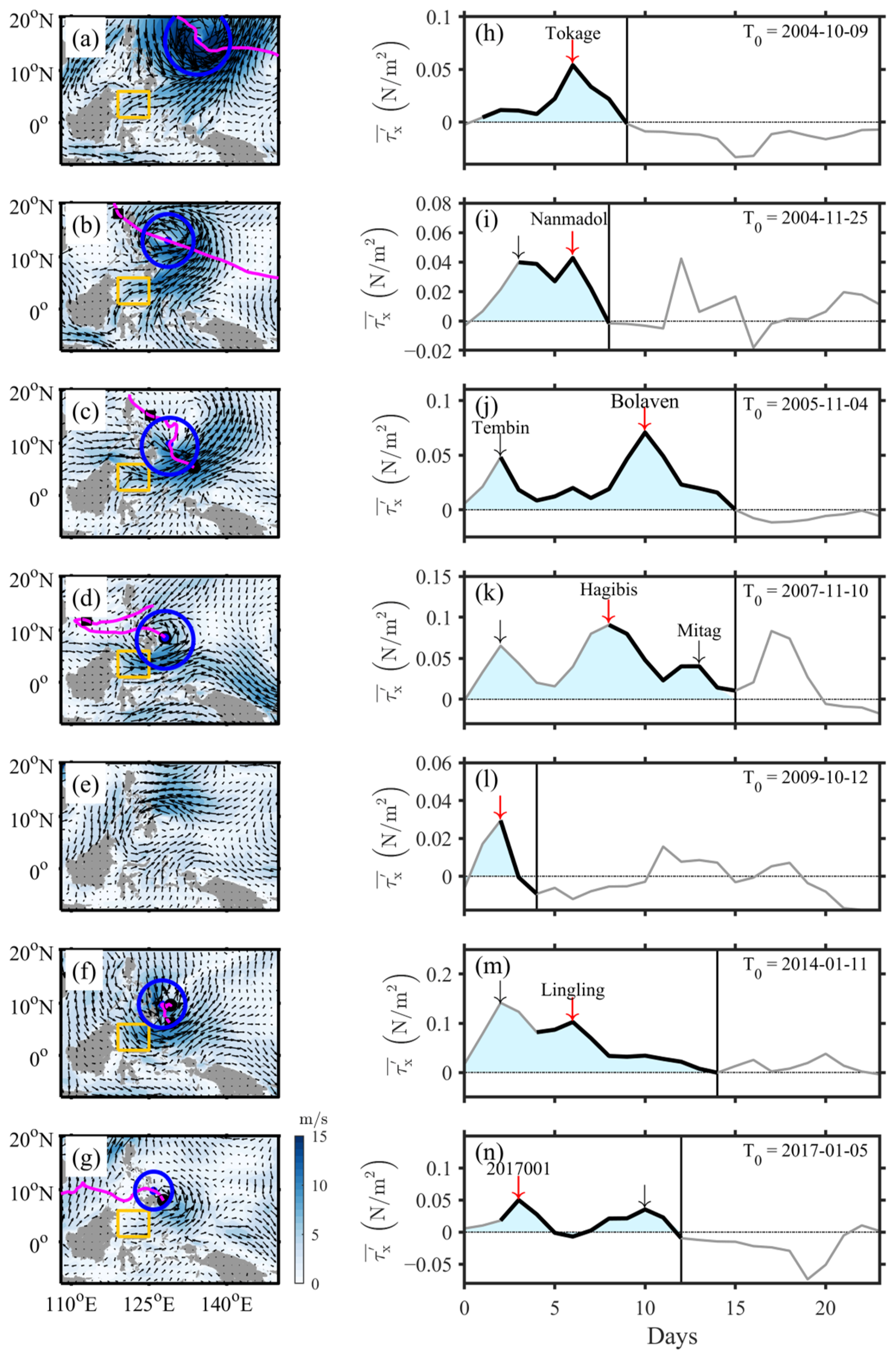
In this study, the events of TCs were first selected according to the zonal wind stress anomaly ${\tau }_x^{\prime }$ of the Sulawesi Sea. The criterion for selection is that the spatially averaged ${\tau }_x^{\prime }$ in the local region exceed 0.032 N m⁻², which is 2 standard deviations of the anomaly. Then, the TCs were further screened based on the incurred variation in surface ITF that must be relative to the time T₀, which represents the starting time of the zonal wind stress anomaly $\overline{{\tau }_x^{\prime }}$ (a spatial average of ${\tau }_x^{\prime }$) in the Sulawesi Sea. The TCs all lead to a reduction in ITF transport, but to a varying extent. We only chose the scenarios of ITF variations based on the following: (1) the time of the first peak in the negative transport anomaly $T_{peak}$ appears within 15 days after T₀, and (2) the negative transport anomaly at time $T_{peak}$ is greater than 0.5 Sv. Among the 56 TCs passing through the selected region from 2004 to 2016 (except for the years with no observations, 2012 and 2013), 13 TCs had strong winds in the Sulawesi Sea associated with them, which corresponded to 10 cases of observed ITF variations (Figure 1). In addition, there was one more case involving a low-pressure system.

Notably, the intraseasonal variability of surface ITF can be a combination of multiple forcing factors, including TCs and MJOs. We determined the MJOs in ONDJF with the method described by Napitu et al. [19]. For this method, three criteria are used, as follows: (1) the filtered outgoing longwave radiation (5° N–5° S average) must exhibit a −10 W/m² contour band between 95° E and 135° E; (2) the amplitude of the Real-time Multivariate MJO (RMM) index [35] must be >1 during phases 4–5 over Indonesia; and (3) the zonal wind stress in the southern Makassar Strait must exceed 0.02 N/m² to define the MJO events affecting the Indonesian Sea. Based on these criteria, 7 TC events occurred without a concurrent MJO, and 4 TC events occurred with a concurrent MJO. The focus of the present study is to identify the impact of TCs on the ITF. Therefore, only cases without a concurrent MJO were selected for study.

Figure 2 shows the moving path of the selected TCs since they were named and the corresponding time series of $\overline{{\tau }_x^{\prime }}$ in the Sulawesi Sea. At the time of maximum $\overline{{\tau }_x^{\prime }}$, the TCs all feature a radius that is smaller than the distance between the center of the TC and the Sulawesi Sea (Figure 2). However, they forced significant meridional wind stress in the Sulawesi Sea. So, the timestamps of the TCs are based on the wind stress anomalies in the Sulawesi Sea and are listed in

Table 1. The start time (UTC) of the Sulawesi Sea wind stress anomaly (T₀) during the TCs and the associated time (in days) for $T_{\mathrm{m}\mathrm{a}\mathrm{x}}\left(\overline{{\tau }_x^{\prime }}\right)$ (time of the maximum $\overline{{\tau }_x^{\prime }}$), T₁, and T_peak.

	TC Name	T0	${\mathit{T}}_{\mathbf{m}\mathbf{a}\mathbf{x}}$($\overline{{\mathit{\tau }}_{\mathit{x}}^{\mathbf{\prime }}}$)	T1	Tpeak
1	Tokage	9 October 2004	6	9	8
2	Nanmadol	25 November 2004	6	8	8
3	Bolaven	4 November 2005	10	15	13
4	Hagibis	10 November 2007	8	15	14
5	N/A	12 October 2009	2	3	-
6	Lingling	11 January 2014	6	9	11
7	2017001	5 January 2017	3	12	13

. The durations of MJOs with concurrent TCs are listed in

Table 2. Winter MJO events from 2004 to 2017 (except 2012–2013) in the Indonesian Sea.

	MJO in the Indonesian Sea	TC Name
1	6 December 2005–12 February 2006
2	20 March 2006–5 April 2006
3	5 December 2007–17 January 2008
4	24 January 2008–28 February 2008
5	4 November 2009–1 December 2009
6	23 December 2009–21 January 2010	2009091
7	13 January 2011–4 February 2011
8	22 November 2014–9 December 2014	Hagupit
9	16 December 2014–12 January 2015	Jangmi
10	7 December 2015–27 December 2015	Melor, 2015109
11	30 January 2016–19 February 2016
12	18 January 2017–13 February 2017

for reference.

2.2. Ocean Reanalysis

Owing to a lack of data collection at depths above 40 m, the analysis of the observed surface ITF transport is underestimated. A more accurate estimate was made using the eddy-resolving global ocean reanalysis (GLORYS12v1 [35,36], product ID: GLOBAL_MULTIYEAR_PHY_001_030) from the surface to 100 m deep. The GLORYS12v1 reanalysis was published by the Copernicus Monitoring Environment Marine Service (CMEMS). The daily averaged model output has a horizontal resolution of 1/12° and 50 layers in the vertical direction. The model was configured with a high resolution in the surface layer (25 model layers in the upper 150 m, and the thickness of the first layer is approximately 0.5 m) to resolve the upper-ocean dynamics.

2.3. Numerical Model of the ITF

A regional circulation model with high resolution in the Indonesian seas was established using FVCOM [37]. The model has a large domain across the Pacific and Indian Oceans, which is enough for the assessment of oceanic response to TCs. Horizontally, unstructured grids of 3 km in length were designed to adequately resolve the circulations across the narrow straits of this region. Vertically, the model employed a 68-layer terrain-following sigma coordinate, with enhanced resolution near the surface to capture the mixed layer dynamics and thermocline structure. The bathymetric data of the model were derived from the global 30 arc-second dataset of GEBCO [38]. The vertical mixing processes were parameterized using the turbulence closure scheme described in Umlauf and Burchard [39].

The model used the HYCOM reanalysis fields [40] as the initial conditions to conduct the simulation with realistic ocean circulation. Tides, including the open-boundary tides and astronomical tides, have been turned on for the model states to reach a quasi-equilibrium quickly. The tidal elevation and currents at the open boundary are predicted by TPXO8.0 [] with eight constituents (M₂, S₂, N₂, K₂, K₁, P₁, O₁, and Q₁). The sub-tidal components of surface elevation and 3D variables, including temperature, salinity, and currents at the open boundary, are interpolated from HYCOM. The surface boundary conditions of the model were forced by the hourly reanalysis data from the Climate Forecast System version 2 (CFSv2, [41]). The momentum and heat fluxes were computed in the model through the COARE3.5 bulk aerodynamic formula. Notably, the model has a climatological monthly freshwater discharge from 608 rivers to account for the terrestrial hydrological influences.

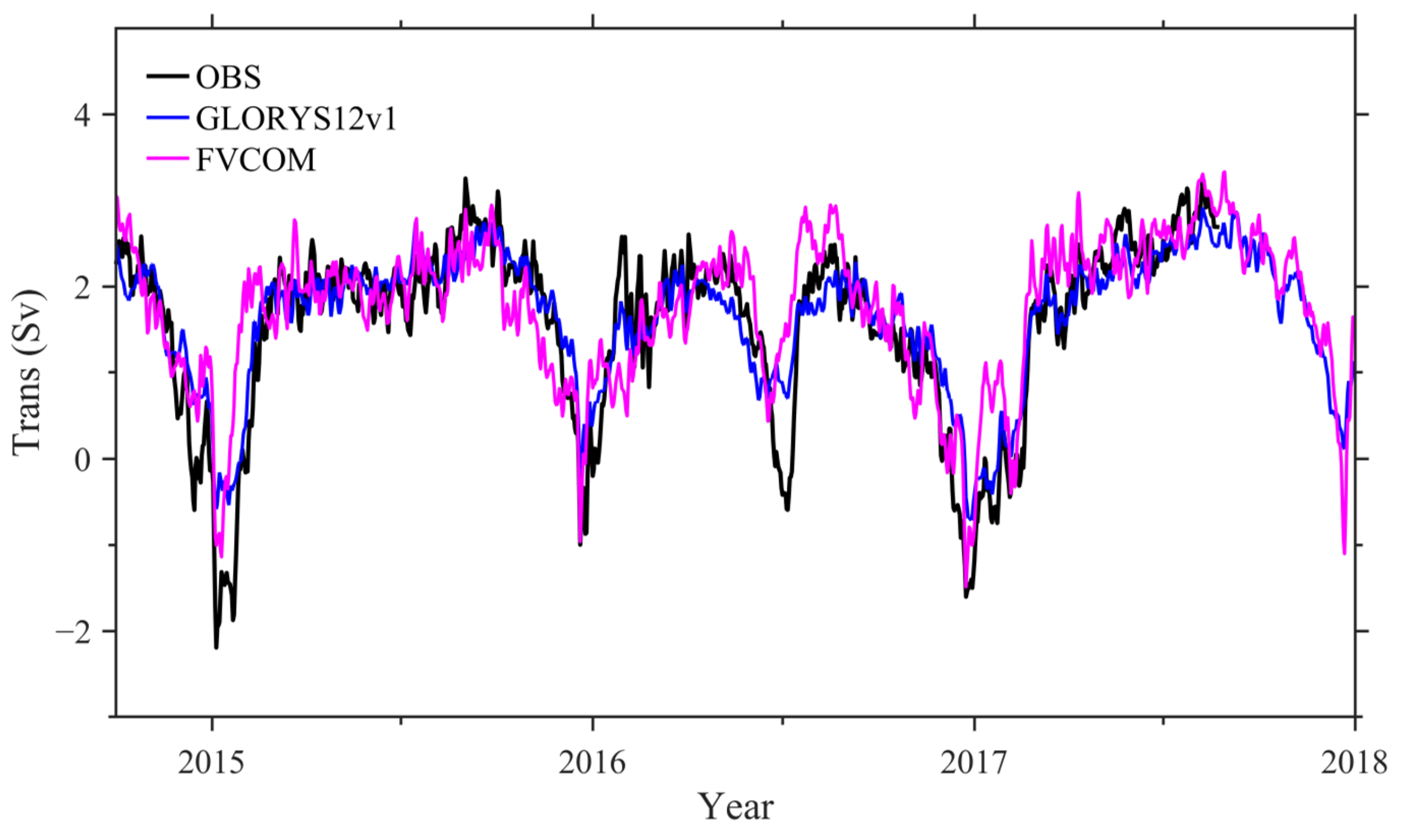
The model simulation of the Makassar Strait throughflow transport at the surface layer has been validated against the observations from 2015 to 2018 (Figure 3). A comparison was also made between the model and GLORYS12v1 reanalysis data. Generally, the model prediction of the surface ITF transport matches well with both the observations and the reanalysis data. In contrast, the model has a difference with the observations that is slightly larger than that of the reanalysis data. The relative error is 23% in the model, while it is 17% in the reanalysis. The RMSE is 0.57 Sv in the model, while it is 0.23 Sv in the reanalysis.

2.4. Twin Experiments to Isolate the TC Forcing on ITF

Twin numerical experiments were conducted using the established FVCOM model to isolate the impact of TCs on ITF variability. For each TC event, the realistic model simulation started two months before the time T₀ and continuously ran for an additional two months after T₀. The parallel simulation was driven by the same forcing as the realistic run, except that the winds of the TC have been removed. Thus, the difference between the parallel model simulations represents the impact of TCs on ITF.

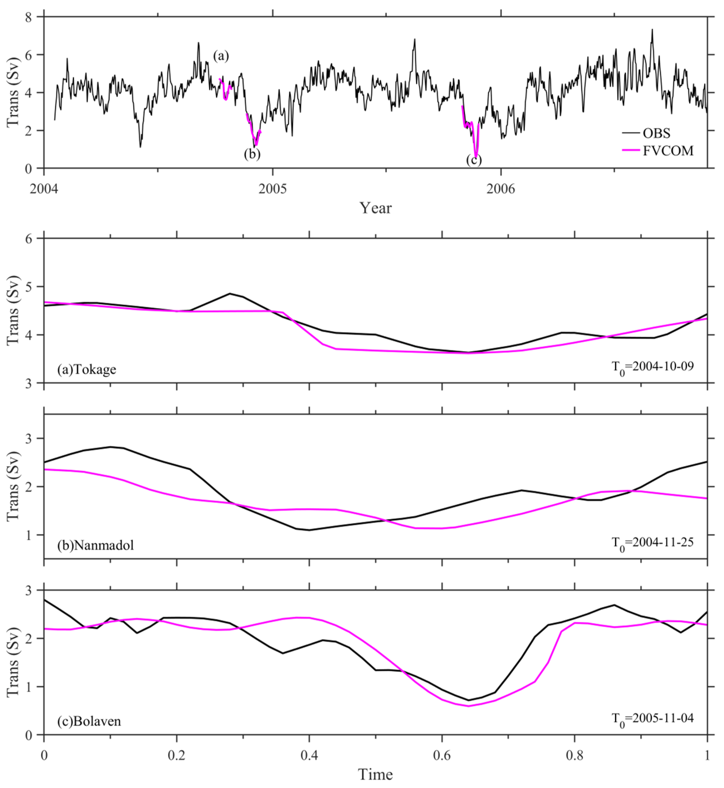
Before the twin experiments, the simulations of ITF transport (40–100 m) with the TC forcing have been validated. The correlation between the model simulations and observations is in the range of 0.6–0.88 and, on average, 0.73 for all the cases. In addition to that, the simulations of the full surface ITF transport (0–100 m) with the TC forcing were validated using the ADCP data from the INSTANT project in the years 2004–2006. As shown in Figure 4, the prediction of the ITF transport variation matches well with the observations. The RMSE is 0.22 Sv, 0.34 Sv, and 0.42 Sv in the events of TCs Tokage, Nanmadol, and Bolaven, while the corresponding Scatter Index value is 0.05, 0.16, and 0.19, respectively. The low values of RMSE and Scatter Index demonstrate the robustness of the model results to reproduce the basal transport and variation in ITF forced by the TCs.

To isolate the winds in the TC circulation, we implemented the analyzed vortex removal method described by Kurihara et al. [42]. The procedure involves a decomposition of the original scalar fields h(x,y,t) (including atmospheric pressure and zonal and meridional components of winds) into a basic field h_B(x,y,t) and a disturbance field h_D(x,y,t) using a local three-point smoothing filtering operator:

$$h(\mathrm{x},\mathrm{y},\mathrm{t})=h_B(\mathrm{x},\mathrm{y},\mathrm{t})+h_D(\mathrm{x},\mathrm{y},\mathrm{t})$$

(1)

Subsequently, a cylindrical filter is applied to isolate the analyzed vortex component h_av(x,y,t) from h_D(x,y,t), yielding a non-TC perturbation h_non:

$$h_D(\mathrm{x},\mathrm{y},\mathrm{t})=h_{\mathrm{a}\mathrm{v}}(\mathrm{x},\mathrm{y},\mathrm{t})+h_{\mathrm{n}\mathrm{o}\mathrm{n}}(\mathrm{x},\mathrm{y},\mathrm{t})$$

(2)

The background atmospheric field h_bg(x,y,t) is then reconstructed by recombining h_non(x,y,t) with the basic field h_B(x,y,t):

$$\begin{gathered} h_{\mathrm{b}\mathrm{g}}\left(\mathrm{x},\mathrm{y},\mathrm{t}\right)=h_B\left(\mathrm{x},\mathrm{y},\mathrm{t}\right)+h_{\mathrm{n}\mathrm{o}\mathrm{n}}\left(\mathrm{x},\mathrm{y},\mathrm{t}\right) \\ =h_B\left(\mathrm{x},\mathrm{y},\mathrm{t}\right)+\left(h_D\left(\mathrm{x},\mathrm{y},\mathrm{t}\right)-h_{\mathrm{a}\mathrm{v}}\left(\mathrm{x},\mathrm{y},\mathrm{t}\right)\right) \\ =h\left(\mathrm{x},\mathrm{y},\mathrm{t}\right)-h_{\mathrm{a}\mathrm{v}}\left(\mathrm{x},\mathrm{y},\mathrm{t}\right) \end{gathered}$$

(3)

To eliminate the Sulawesi Sea’s winds forced by the TCs, the removal radius R for h_av needed to be enlarged beyond the radius of the TCs. A spatial buffer zone, which starts from 0.5R, was used to mitigate the discontinuities between the background field and original scalar fields. Temporally, a 24 h transition time is specified before T₀ and after T₁ to ensure that the atmospheric forcing is changed gradually. It is required to reduce the impact of the forcing perturbation on the numerical stability of the ocean model.

2.5. Along-Strait Momentum Budget Analysis

To quantitatively evaluate the relative contributions from local wind forcing and surface pressure gradients to the northward velocity anomalies in the Makassar Strait, an along-strait momentum budget analysis was conducted by adopting a simplified equation for horizontal momentum conservation integrated over the surface layer. Following the work of Napitu et al. [19] and Xu et al. [43], the equation is as follows:

$${\displaystyle \frac{\partial \overline{v}}{\partial \mathrm{t}}}+f\overline{u}=-g{\displaystyle \frac{\partial {\eta }^{\prime }}{\partial y}}+{\displaystyle \frac{{\tau }_y}{\rho H}}+\mathrm{R}\mathrm{e}\mathrm{s}$$

(4)

where the y-axis is parallel to the along-strait axis in the Makassar Strait. H = 100 m is the surface layer thickness, $\overline{v}={\displaystyle \frac{1}{H}}{\int }_0^{H}vdz$ and $\overline{u}={\displaystyle \frac{1}{H}}{\int }_0^{H}udz$ are the vertically averaged along-strait and cross-strait velocities at the mooring site derived from the reanalysis, f is the Coriolis parameter, η′ represents the sea level anomaly, $g$ is gravity, ${\tau }_y$ indicates the along-strait wind stress, $\rho$ is the background density (1023 kg/m³), and Res is the residual. In Formula (4), the magnitude of the Coriolis force is on the order of 10⁻⁸ m/s², which is smaller than the other dominant balancing terms. Therefore, the Coriolis force term is ignored in the following analysis.

2.6. The Linear Kelvin Wave Model

The analytical linear Kelvin wave model is adopted from Xu et al. [44], which is based on the work of Gill [45], to simulate the Kelvin wave propagation from the Equator in the Indian Ocean into the Makassar Strait. Each mode of the Kelvin waves SLA_n is calculated individually as follows:

$${\mathrm{S}\mathrm{L}\mathrm{A}}_n\left(x_0,t\right)={\alpha }_n{\int }_A^L{\tau }_x\left(x,t+{\displaystyle \frac{x-x_0}{c_n}}\right)\mathrm{d}x$$

(5)

where ${\alpha }_n$ is the corresponding signal coefficient for the nth mode of the simulation. According to Xu et al. [44], ${\alpha }_n={\psi }_n^2\left(0\right)/\rho gD$, where ${\psi }_n\left(0\right)$ is the value of the Kelvin wave vertical eigenfunction at the sea surface, and D is the bottom depth. ${\tau }_x$ is the TC wind stress along the Kelvin waveguide from the Sulawesi Sea to the Makassar Strait. $c_n$ is the Kelvin wave speed and is set to be 2.8 m/s and 1.8 m/s for the first two baroclinic modes. The Kelvin wave vertical eigenfunction is ${\psi }_n\left(z\right)$ [44,46] writes as

$${\displaystyle \frac{\partial }{\partial z}}\left[{\displaystyle \frac{1}{N^2\left(z\right)}}{\displaystyle \frac{\partial {\psi }_n(z)}{\partial z}}\right]=-{\displaystyle \frac{1}{c_n^2}}{\psi }_n\left(z\right)$$

(6)

with the boundary condition at the sea surface and bottom satisfying

$${\displaystyle \frac{\partial {\psi }_n\left(0\right)}{\partial z}}={\displaystyle \frac{\partial {\psi }_n\left(D\right)}{\partial z}}=0$$

(7)

The ${\psi }_n\left(z\right)$ is normalized, such that

$${\int }_{-D}^0{\psi }_n^2\left(z\right)\mathrm{d}z=D$$

(8)

where $N\left(z\right)$ is the Brunt–Väisälä buoyancy frequency.

3. Results

3.1. Characteristics of the TC Impact on the ITF Transport Variation

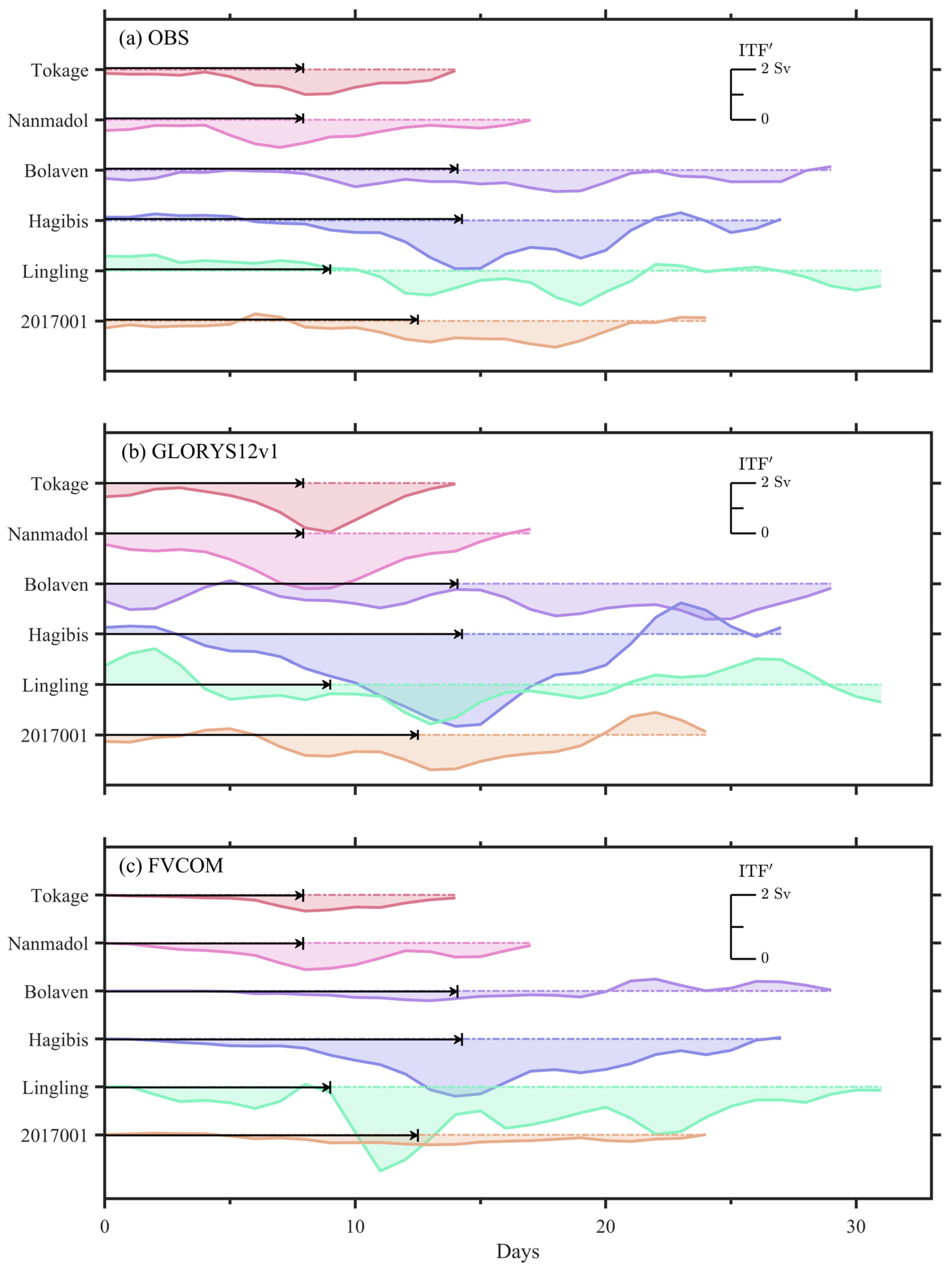
The duration of the TC impact on ITF is determined based on the numerical experiments to isolate the TC forcing on ITF. It is defined as the elapsed time after T₀ until the transport anomaly forced by the TCs disappears. In the model, the variability of surface ITF generally features a reduction and a recovery phase (Figure 5c, except for the TC in October 2009, because it had a weak wind pattern, making it difficult to isolate from the surrounding atmospheric circulations). After that, the variation becomes much weaker and diverges among the cases. In the observation, the ITF transport anomaly associated with the TCs is determined based on the same variation pattern (Figure 5a). The correlation between the model and observation is as high as 0.7, above the 95% significance level. The same method is also used to determine the ITF transport anomaly in the reanalysis (Figure 5b). A match between the observations and simulations supports that the TCs have the primary impact on the ITF transport variation during this period.

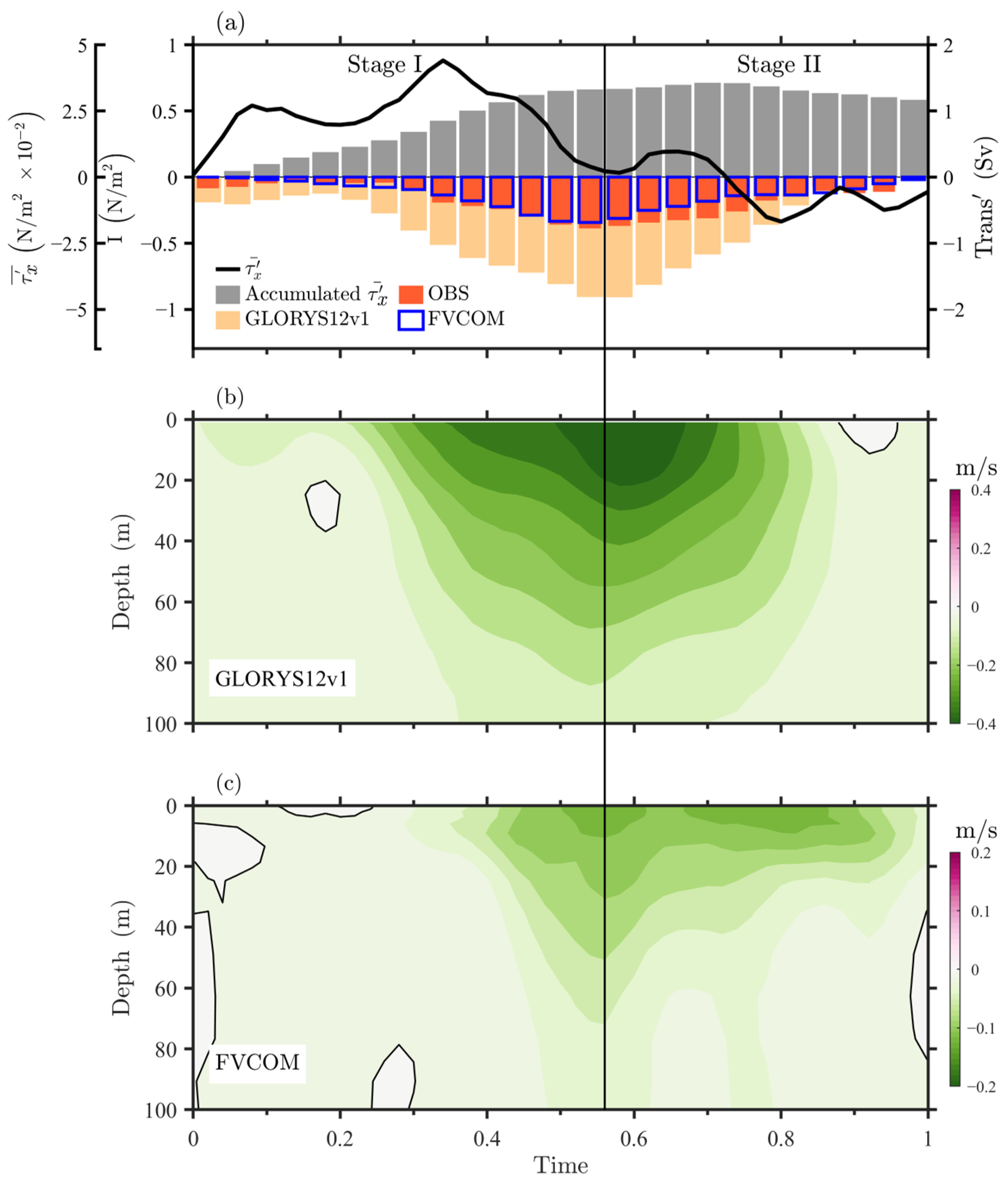
A composite analysis was performed during the Tokage, Nanmadol, Bolaven, Hagibis, and 2017001 TCs (note that TC Lingling was not included, as explained later). The two periods of variation since time T₀: the reduction phase (Stage I) and the recovery phase (Stage II), are clearly shown (Figure 6a). In Stage I, the ITF is affected by the winds of the TCs. A maximum magnitude of transport reduction occurs at the end of Stage I. TC Lingling is a special case since the maximum magnitude of transport reduction appeared in Stage II instead of in Stage I. It is verified in the numerical experiments and may be due to the uniqueness of the TC’s moving path since it moved slowly and was confined to the east side of Mindanao Island (Figure 2). On average, Stage I took approximately 12 days among all of the cases, but a maximum of 15 days was observed for Bolaven and Hagibis TCs (Figure 5). In Stage II, the negative transport anomaly did not diminish immediately and gradually decreased until it completely disappeared. This process takes another 5–15 days, so the total duration of the ITF transport variation is up to 30 days.

In the observations, the average transport reductions for Stages I and II were 0.31 ± 0.09 Sv and 0.41 ± 0.13 Sv, respectively. However, the full surface layer estimations from the reanalysis approximately doubled (0.85 ± 0.36 and 0.76 ± 0.29 Sv, respectively). The lack of data collection at depths above 40 m causes ~46% underestimation in the observation if an 18% error in the difference between the observation and reanalysis is accounted for [47]. Based on the numerical experiments, the impact of TCs from the upstream region of the Sulawesi Sea contributes ~40% to the total ITF transport reduction during this period.

The vertical structure of the flow anomaly from the reanalysis verifies that the weakening of ITF mainly occurs at the surface layer of the water column (Figure 6b). The numerical experiments with/without the TC wind forcing produce a smaller magnitude but similar structure of the flow anomaly (Figure 6c). The difference between the results indicates that the influence of TCs on ITF is larger than the wind impact from the upstream region of the Makassar Strait.

3.2. Surface Ocean Dynamics During and After the TCs

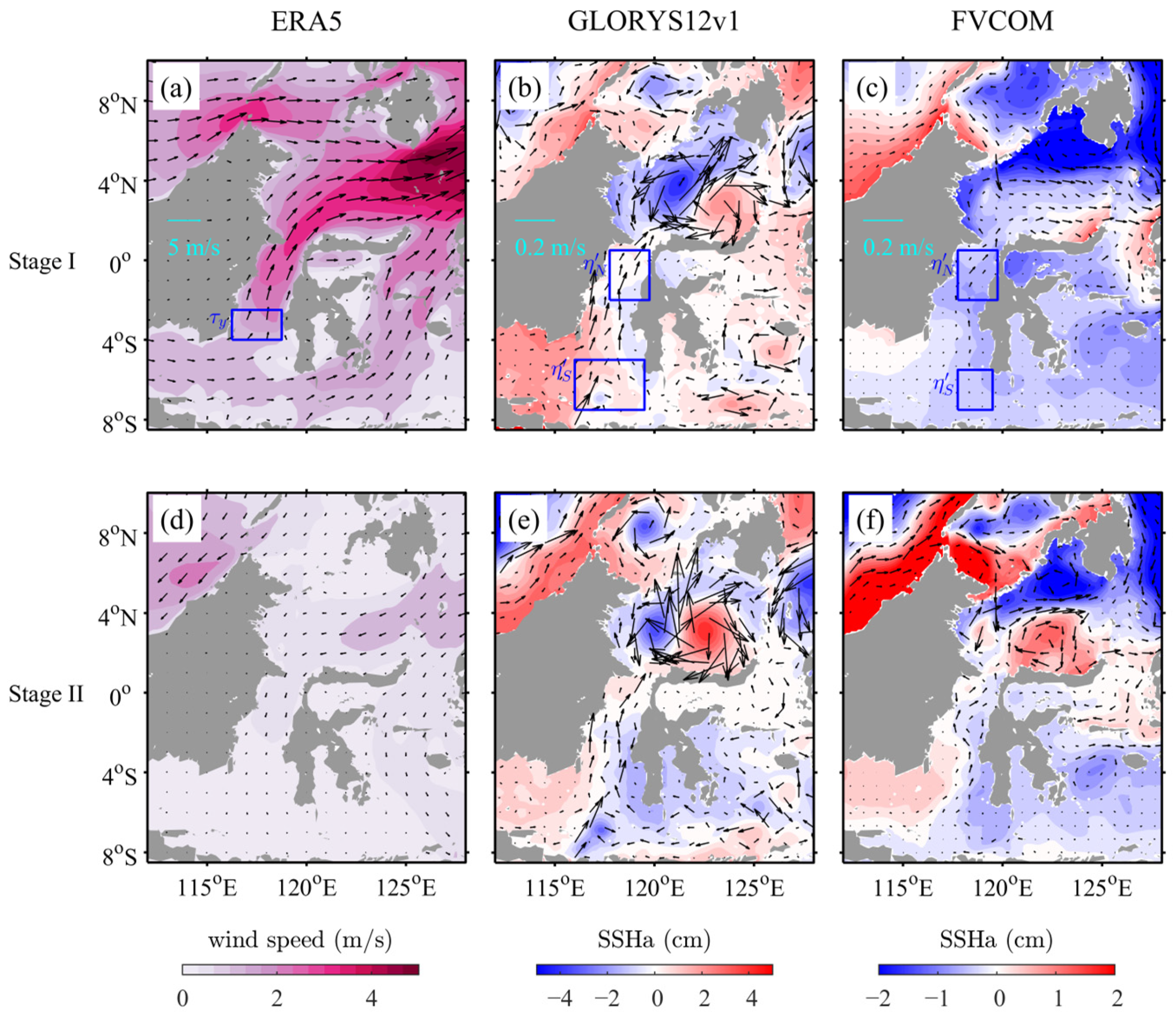
Surface ocean dynamics during and after the TCs are presented in Figure 7 over the Indonesian Sea. In Stage I, the circulation of TC drives a strong eastward wind stress anomaly in the Sulawesi Sea. During this time, the surface elevation has a main north–south gradient across the basin, but the low sea level along the basin’s northern coast further extends to the western coast and can reach the entrance of the Makassar Strait (Figure 7c). Under the TC forcing, the surface layer of circulation in the basin features a net outflow of water to the Pacific Ocean. It may be related to the northward flow anomaly in the Makassar Strait, since a cross-basin sea level difference has been established at that time between the two regions. In Stage I, the guiding circulation surrounding the TCs forces a local wind in the Makassar Strait and Java Sea, but at a decreased strength (Figure 7a). According to the reanalysis, this broader wind influence of the TCs could drive an even stronger northward flow anomaly in the Makassar Strait (Figure 7b). So, the local wind in the Makassar Strait forced by the TCs should be influential on the ITF since it is northward and can contribute to the weakening of the southward surface flow. In addition, the local wind in the Java Sea forced by the TCs may also contribute to the reduction of the ITF transport if a higher sea level in the southern part of the Makassar Strait can be set up by the winds simultaneously.

In Stage II, the relaxation of the TC forcing leads to an adjustment in the regional surface ocean dynamics. Without the impact of winds in the Sulawesi Sea, the adjustment is most significant to the southern half of the basin (Figure 7f). The resulting anticyclonic eddy is situated in the pathway of the previously established northward flow anomaly from the Makassar Strait to the Sulawesi Sea and may eventually contribute to the breakup of the flow. Wind relaxation in the Makassar Strait and Java Sea results in oceanic adjustments locally. These adjustments feature an along-strait sea level gradient change, which conversely contributes to the weakening of the northward flow anomaly in the Makassar Strait (Figure 7e).

3.3. Roles of the Sea Level Variability and Local Winds in the ITF Transport Reduction

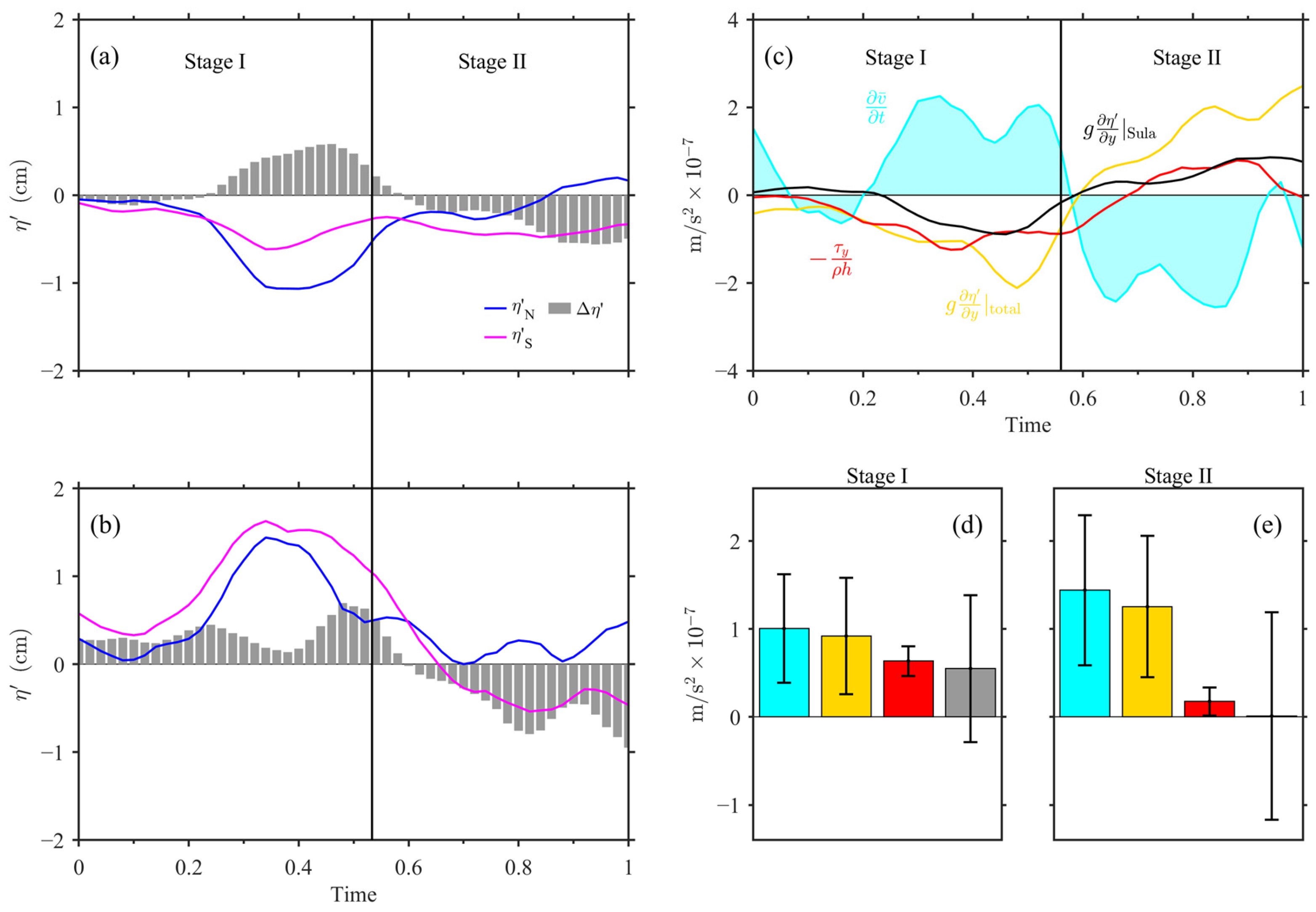
Both the local winds and along-strait pressure gradients can contribute to the weakening of the surface ITF transport in the Makassar Strait. In Figure 8a,b, the sources of the along-strait pressure gradients during the TCs are illustrated. Specifically, two box regions of sea level anomaly in the northern and southern Makassar Strait were selected to evaluate the along-strait pressure gradients. In Stage I, there is a persistent positive surface pressure gradient force (pointing toward the north) in the reanalysis, which can be associated with the northward flow anomaly in the Strait (Figure 8a). The positive values of the sea level anomaly and the higher sea level in the southern Makassar Strait indicate that the driving of the sea level variability is from the downstream region of the Sulawesi Sea. In the FVCOM simulations to isolate the TC wind forcing from the upstream region of the Makassar Strait, a similar positive along-strait pressure gradient force is predicted (Figure 8b). However, it is formed differently compared to the sea level change in the reanalysis because of the negative values of the sea level anomaly and the lower sea level in the northern Makassar Strait. Since only the winds in the Sulawesi Sea and the Pacific Ocean associated with the TCs have been removed in this case, the driving of the sea level variability has to be from the upstream region of the Sulawesi Sea. In Stage II, the along-strait pressure gradient has been reversed, associated with the relaxation of the TC wind forcing.

To assess the relative contribution from local winds and along-strait pressure gradients to the northward flow anomaly in the Makassar Strait, an along-strait momentum budget analysis was conducted over the surface layer. According to the momentum budget analysis, both the local winds and along-strait pressure gradients contribute equally to the transport reduction during the period of wind growth (normalized time < 0.4) (Figure 8c). After that, the effect of local winds on the northward flow anomaly gradually disappears. However, the along-strait pressure gradients further contribute to it. On average, the along-strait pressure gradient is more important than the local winds for driving the northward flow anomaly and weakening the ITF transport during Stage I (Figure 8d). In Stage II, the recovery of the transport is controlled by the reversal of the along-strait pressure gradients, which are due to adjustments in the ocean dynamics after the wind relaxation (Figure 8e).

3.4. Driving Mechanism of the Sea Level Variability by TC Winds from the Upstream Region

The currents and sea level variability in the Indonesian seas can be significantly affected by Kelvin waves propagating into this region from both the Pacific and Indian Oceans [34,48,44]. In Stage I, the low sea level anomaly (SLA) extending along the coast of the Sulawesi Sea is a sign of the coastal Kelvin waves generated by the TC winds, which can reach the northern Makassar Strait by propagating along the north coast of the Sulawesi Sea and subsequently modulate the sea level in the Strait.

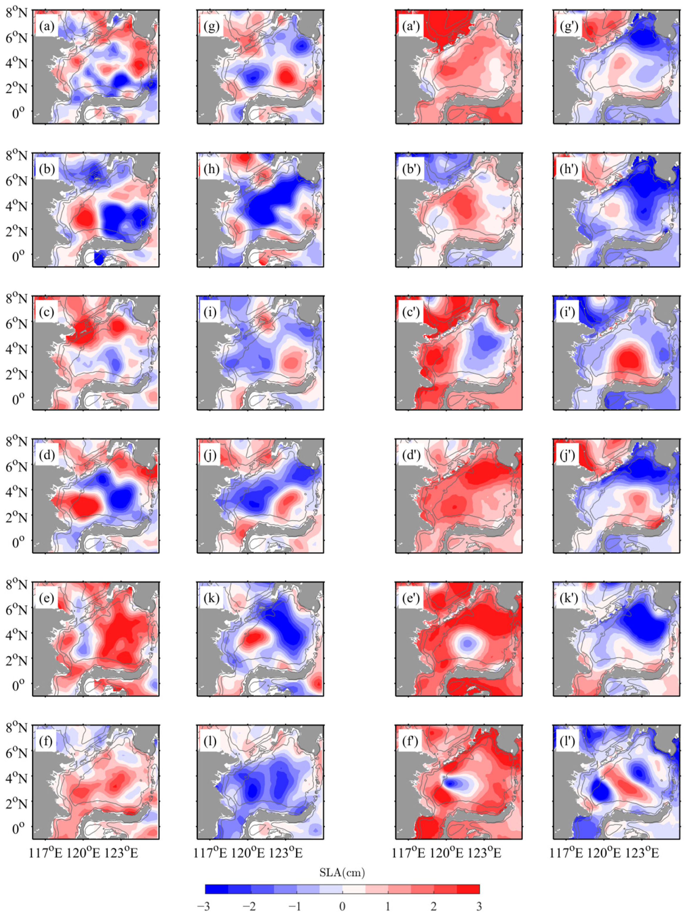
Then, we validate the SLA generated by the model against the AVISO satellite altimetry data during the events. For each case, the average field of SLA over the duration of TC impact (phase 2) is displayed in Figure 9, while the average field of SLA one week before the event (phase 1) is also shown in the figure as a reference. In phase 1, the model simulation has a basin-wide positive SLA in the Sulawesi Sea. It is distinctly different from the spatial pattern of the SLA in phase 2, which features a negative SLA along the north coasts of the Sulawesi Sea, extending westward from the eastern opening of the basin to the northern section of the Makassar Strait. In the observations, a similar transition in the SLA from phase 1 to phase 2 is found. In comparison, the model is reasonably good at reproducing the spatial pattern of SLA in the observations, given that the satellite altimetry data is a 7-day-based composition of along-track data and may contain a relatively large uncertainty in the nearshore region.

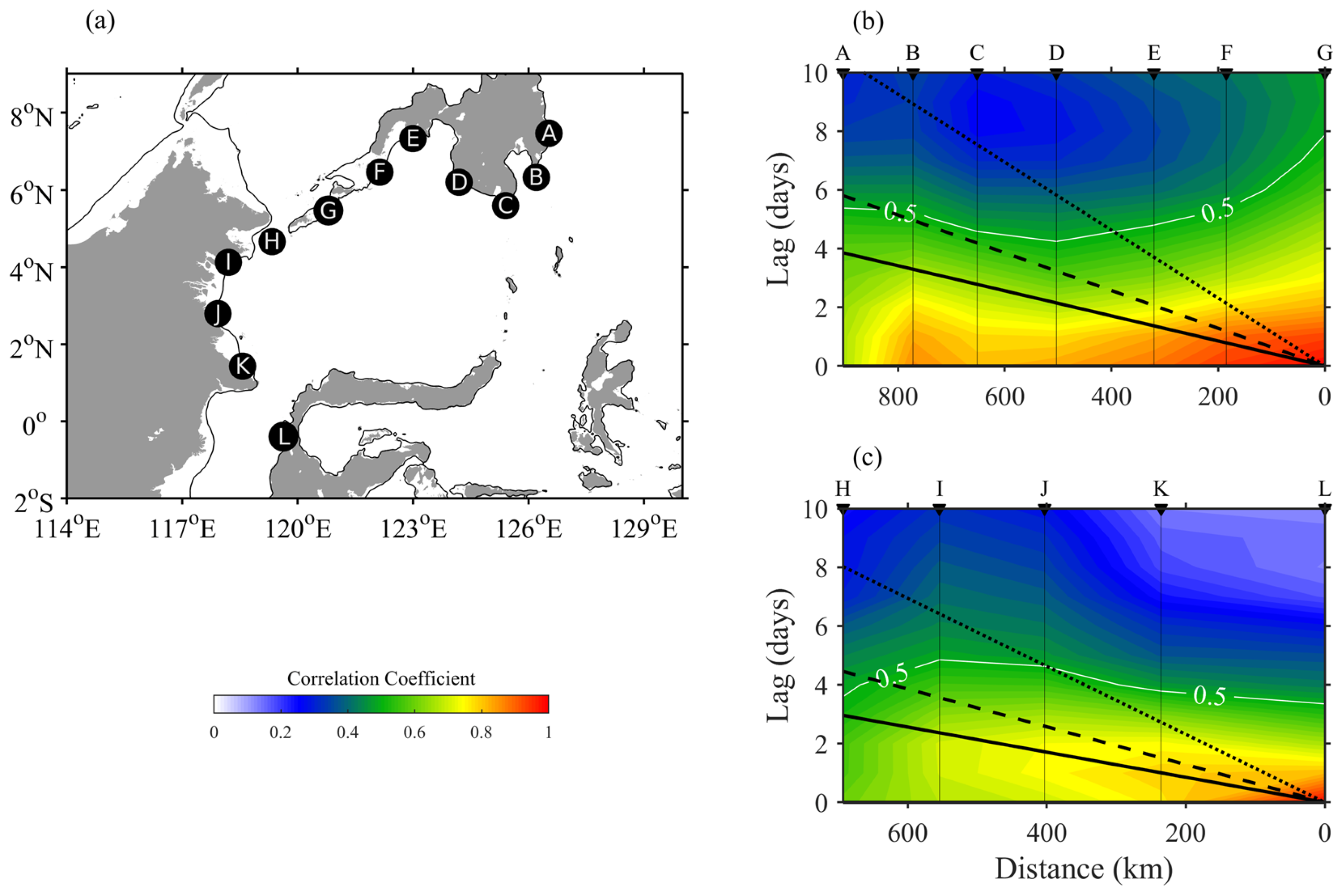
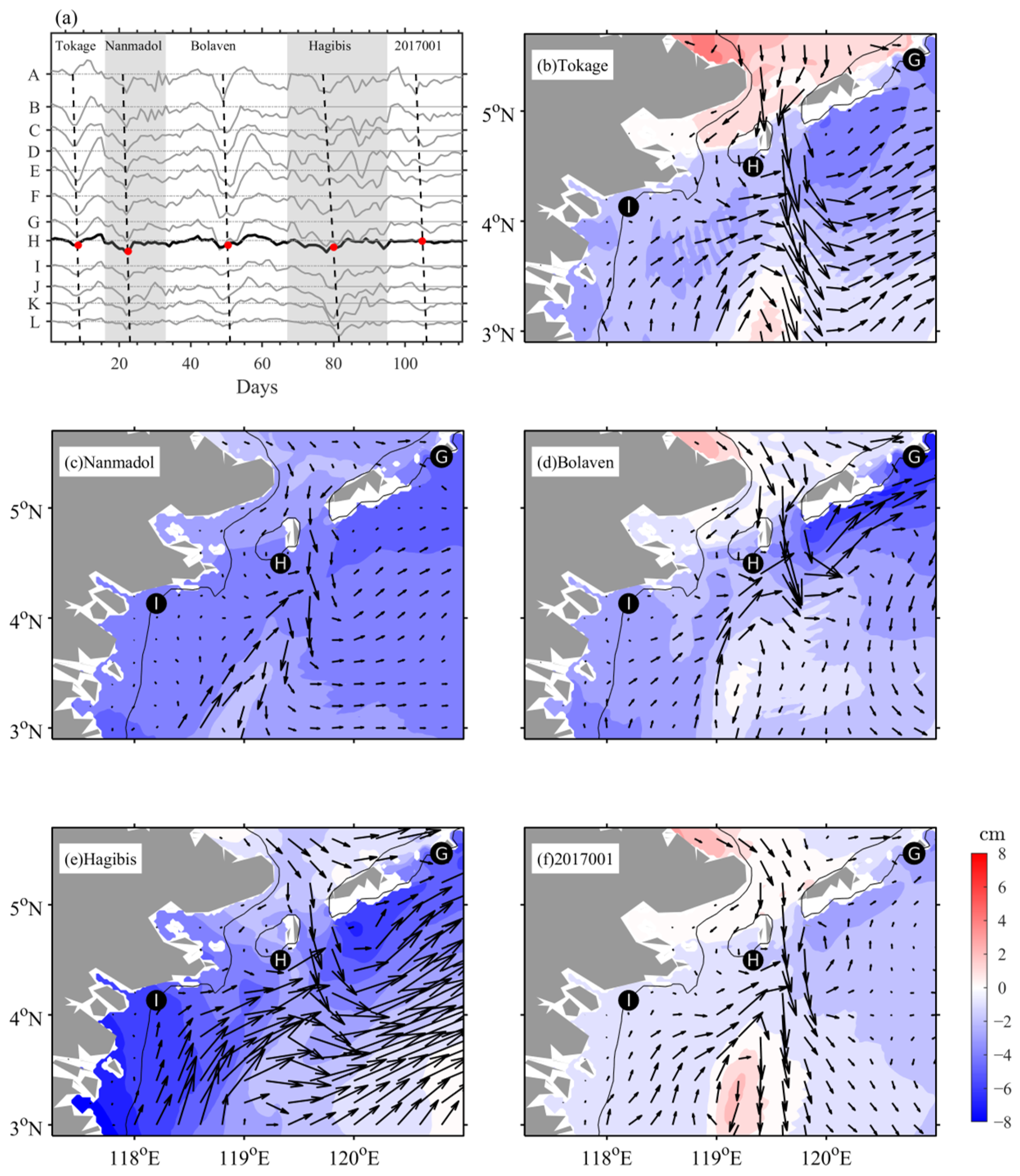
To verify the propagation of coastal Kelvin waves into the Sulawesi Sea, we used the method of Hu et al. [48] to determine the waveguide pathway during the TCs. Here, the analysis is based on the results of FVCOM simulations, which ensures that only the impact of the TCs through the Sulawesi Sea is examined. As shown in Figure 10a, the pathway was divided into two parts (A-G, H-L) because the SLA at point H is subject to the local influence of outflow from the Sulu Sea. The composite analysis shows that during all the TC events, the lag correlation of the SLA between successive points A-G is high (>0.5) (Figure 10b). The slope of the highest correlation in space and with time lag indicates the propagation of Kelvin waves into the Sulawesi Sea with the speed of the first baroclinic mode. The lag correlation of SLA is still high between points H-L (Figure 10c). However, the outflow from the Sibutu passage may influence the further propagation of the Kelvin waves to the northern Makassar Strait. Figure 11 shows that the low sea level feature of wave propagation suddenly disappears at point H and reappears at downstream points in the events of the TCs, and this discontinuity in correlation is associated with the high sea level anomaly along the west coast of the Sulu Sea, which may extend to point H and obscures the low sea level feature of Kelvin wave propagation.

The arrival of Kelvin waves at the northern Makassar Strait through the Sulawesi Sea is further verified using the solutions of the first two baroclinic Kelvin wave modes [48] and the TC wind forcing derived from the ERA5 (same as the winds used in the numerical experiments).

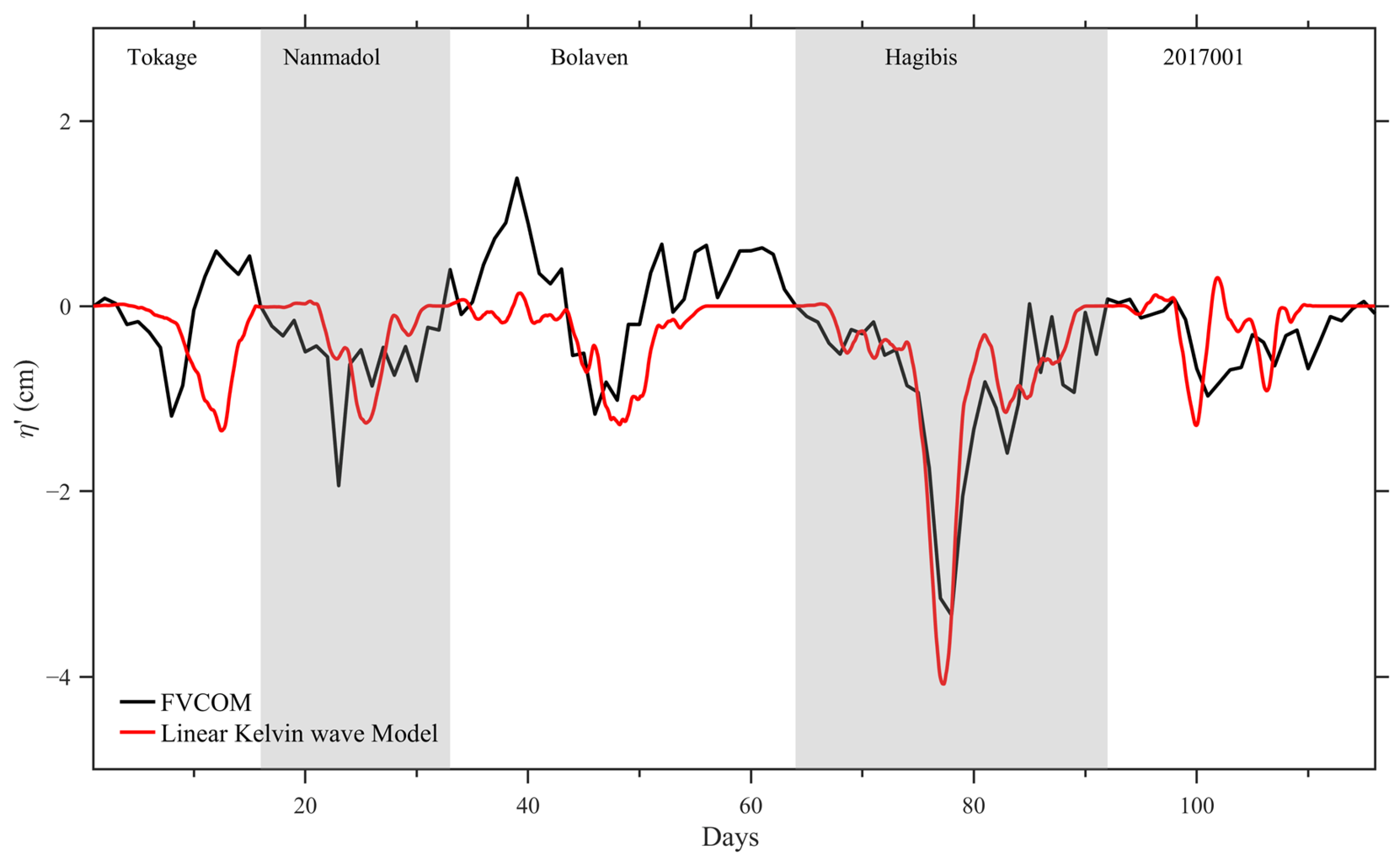
As shown in Figure 12, the negative anomaly of SLA at point L is well predicted by the linear Kelvin wave model. The theoretical prediction of the SLA time series has a reasonably good agreement with the FVCOM simulations during the TC events. The correlation between the two SLAs during the TCs is as high as 0.66, above the 95% significance level. The difference between the model and the theoretical prediction may be due to the nonlinear effect of currents in the Sulawesi Sea or the outflow from the Sibutu passage that significantly impacts the Kelvin wave propagation.

4. Discussion and Summary

A weakening of the surface ITF (<100 m) was observed in the Makassar Strait during boreal winter in the Northern Hemisphere. This was not caused by MJOs, which are the most common mechanism leading to the intraseasonal variability in the surface ITF, but by the TCs passing through the upstream region of the Sulawesi Sea. From 2004 to 2017 (except for the years with no observations, 2012 and 2013), there were 13/2 TCs among the 56/109 TCs selected in winter (October–February)/March–September that led to a significant surface ITF reduction. Monsoon winds in the Indonesian seas may be responsible for the influence of seasonal dependence, given that the summer monsoon and TCs have opposite wind directions, while the winter monsoon and TCs have the same wind directions in this region, making it easier to drive the surface flow variability by TCs. Additionally, among the five TCs selected to study, TC Tokage and Nanmadol occurred in the El Niño phase, while TC Bolaven and Hagibis occurred in the La Niña phase (TC 2017001 occurred with an ENSO state that is approaching a La Niña phase). In contrast, the TCs that occurred in the La Niña phase tend to be stronger in their influence on the ITF since they featured a moving path that is more southward and closer to the Sulawesi Sea (Figure 2). So, the interannual baseline state of the equatorial Pacific may modulate the influence through a precondition on the TC forcing.

In the observations, the estimated magnitude of the transport reduction is on average 0.31 Sv, which is ~70% of the 0.45 Sv estimation associated with the MJOs [19]. However, the actual magnitude of the decrease may be doubled because the observations did not include data from the upper 40 m of surface water. We compared the difference in the transport between the 40–100 m layer and the full 0–100 m surface layer using the reanalysis data. In contrast, the transport reduction in the 40–100 m layer is approximately 0.28 Sv, slightly weaker than the observations, while the transport reduction in the 0–100 m layer is 0.76 Sv, nearly 2.7 times larger. Thus, the lack of the upper 40 m data may significantly underestimate the impact of TCs on surface ITF. Despite the underestimation in observations, the feature of the variation obtained from the numerical experiments and validated by the observations is robust. The time scale of the involved variation is up to 30 days. This period is much longer than the wind action time of the TCs but is relatively shorter than the 20–90 days of variation time during the MJOs [49]. However, it is worth noting that the small sample size in this study may introduce certain bias into the results. Nevertheless, the magnitude and duration of the TC’s impact determine that the surface ITF transport may be subject to significant change, even without the occurrence of MJOs.

As shown in Table 2, the variation in surface ITF can be affected jointly by the TC and MJO. In such a case, the wind anomaly in the Java Sea may already cause a weakening of the surface ITF by setting up a higher sea level in the southern Makassar Strait. Meanwhile, a lower sea level in the northern Makassar Strait can further weaken the transport, which is associated with the TC forcing to generate the coastal Kelvin wave propagating through the Sulawesi Sea. Although the exact behavior of the interaction is still unknown, the combination of the influences could be nonlinear and lead to the extremely low volume transport of ITF during the boreal winter of 2014/2015.

Napitu et al. [19] reported that the intraseasonal ITF in the Makassar Strait is modulated by remote winds in the Java Sea during the active phase of MJOs. The transport reduction results from an amplified north–south sea surface pressure gradient in the Makassar Strait, and it is the wind stress along the coast of the Java Sea that causes the rise in sea level in the southern part of the Strait.

In the event of TC, the winds inside the TC circulation have a strong impact on the Makassar Strait’s ITF transport from the upstream region and through the Sulawesi Sea. Specifically, coastal Kelvin waves are generated along the Philippine coasts under the wind forcing, which can propagate into the Sulawesi Sea and arrive at the northern Makassar Strait to impact the sea level variability and current. Based on the numerical experiments, this mechanism contributes ~40% to the total ITF transport reduction. During the TCs, the large-scale guiding circulation surrounding the TCs is also influential to the Makassar Strait’s ITF transport. It may involve the role of the local northward wind anomaly forced by the TC in the Makassar Strait and/or of the local winds forced by the TC in the Java Sea, which could affect the along-strait pressure gradients in a way similar to the MJO. In addition, the extreme rainfall associated with the TC may also be a potential candidate for the mechanism to alter the along-strait pressure gradients. However, it is ignored in the present numerical experiments with the climatological river runoff.

Given the interesting findings of the results, future work is needed to thoroughly validate the processes and dynamics of the TC impact on the surface ITF. It thus may require an extension of the hindcasting simulations to increase the sample size, which is helpful to reduce the bias in the present results. It may also require taking more influencing factors, such as the rainfall and ENSO, into consideration, to ensure the robustness of the results.

References

1. Wyrtki, K. Indonesian through flow and the associated pressure gradient. J. Geophys. Res. Oceans 1987, 92, 12941–12946. [Google Scholar] [CrossRef]
2. Du, Y.; Wang, F.; Wang, T.; Liu, W.; Liang, L.; Zhang, Y.; Chen, Y.; Liu, J.; Wu, W.; Yu, K.; et al. Multi-scale ocean dynamical processes in the Indo-Pacific Convergence Zone and their climatic and ecological effects. Earth-Sci. Rev. 2023, 237, 104313. [Google Scholar] [CrossRef]
3. England, M.H.; Huang, F. On the Interannual Variability of the Indonesian Throughflow and Its Linkage with ENSO. J. Clim. 2005, 18, 1435–1444. [Google Scholar] [CrossRef]
4. Gordon, A.L.; Huber, B.A.; Metzger, E.J.; Susanto, R.D.; Hurlburt, H.E.; Adi, T.R. South China Sea throughflow impact on the Indonesian throughflow. Geophys. Res. Lett. 2012, 39, L11611. [Google Scholar] [CrossRef]
5. Yuan, D.; Zhou, H.; Zhao, X. Interannual Climate Variability over the Tropical Pacific Ocean Induced by the Indian Ocean Dipole through the Indonesian Throughflow. J. Clim. 2013, 26, 2845–2861. [Google Scholar] [CrossRef]
6. Sprintall, J.; Révelard, A. The Indonesian Throughflow response to Indo-Pacific climate variability. J. Geophys. Res. Oceans 2014, 119, 1161–1175. [Google Scholar] [CrossRef]
7. Li, M.; Gordon, A.L.; Gruenburg, L.K.; Wei, J.; Yang, S. Interannual to Decadal Response of the Indonesian Throughflow Vertical Profile to Indo-Pacific Forcing. Geophys. Res. Lett. 2020, 47, e2020GL087679. [Google Scholar] [CrossRef]
8. Gordon, A.L.; Napitu, A.; Huber, B.A.; Gruenburg, L.K.; Pujiana, K.; Agustiadi, T.; Kuswardani, A.; Mbay, N.; Setiawan, A. Makassar Strait Throughflow Seasonal and Interannual Variability: An Overview. J. Geophys. Res. Oceans 2019, 124, 3724–3736. [Google Scholar] [CrossRef]
9. Sprintall, J.; Gordon, A.L.; Wijffels, S.E.; Feng, M.; Hu, S.; Koch-Larrouy, A.; Phillips, H.; Nugroho, D.; Napitu, A.; Pujiana, K.; et al. Detecting Change in the Indonesian Seas. Front. Mar. Sci. 2019, 6, 257. [Google Scholar] [CrossRef]
10. Gordon, A.L.; Susanto, R.D.; Vranes, K. Cool Indonesian throughflow as a consequence of restricted surface layer flow. Nature 2003, 425, 824–828. [Google Scholar] [CrossRef]
11. Zhu, Q.; Wang, C. Contributions of Indo-Pacific forcings to interannual variability of the Indonesian Throughflow in the upper and lower layers. J. Geophys. Res. Oceans 2023. [Google Scholar]
12. Hu, X.; Sprintall, J.; Yuan, D.; Tranchant, B.; Gaspar, P.; Koch-Larrouy, A.; Reffray, G.; Li, X.; Wang, Z.; Li, Y.; et al. Interannual variability of the Sulawesi Sea circulation forced by Indo-Pacific planetary waves. J. Geophys. Res. Oceans 2019, 124, 1616–1633. [Google Scholar] [CrossRef]
13. Santoso, A.; England, M.H.; Kajtar, J.B.; Cai, W. Indonesian Throughflow Variability and Linkage to ENSO and IOD in an Ensemble of CMIP5 Models. J. Clim. 2022, 35, 3161–3178. [Google Scholar] [CrossRef]
14. Yuan, D.; Li, X.; Wang, Z.; Li, Y.; Wang, J.; Yang, Y.; Hu, X.; Tan, S.; Zhou, H.; Wardana, A.K.; et al. Observed transport variations in the Maluku Channel of the Indonesian Seas associated with western boundary current changes. J. Phys. Oceanogr. 2018, 48, 1803–1813. [Google Scholar] [CrossRef]
15. Lu, X.; Hu, S.; Guan, C.; Li, M.; Sprintall, J.; Wang, F. Quantifying the Contribution of Salinity Effect to the Seasonal Variability of the Makassar Strait Throughflow. Geophys. Res. Lett. 2023, 50, e2023GL105991. [Google Scholar] [CrossRef]
16. Lee, T.; Fournier, S.; Gordon, A.L.; Sprintall, J. Maritime Continent water cycle regulates low-latitude chokepoint of global ocean circulation. Nat. Commun. 2019, 10, 2103. [Google Scholar] [CrossRef] [PubMed]
17. Susanto, R.D.; Ffield, A.; Gordon, A.L.; Adi, T.R. Variability of Indonesian throughflow within Makassar Strait, 2004–2009. J. Geophys. Res. Oceans 2012, 117, C09013. [Google Scholar] [CrossRef]
18. Pujiana, K.; Gordon, A.L.; Sprintall, J. Intraseasonal Kelvin wave in Makassar Strait. J. Geophys. Res. Oceans 2013, 118, 2023–2034. [Google Scholar] [CrossRef]
19. Napitu, A.M.; Pujiana, K.; Gordon, A.L. The Madden-Julian Oscillation’s Impact on the Makassar Strait Surface Layer Transport. J. Geophys. Res. Oceans 2019, 124, 3538–3550. [Google Scholar] [CrossRef]
20. Nieva Tamasiunas, M.C.; Shinoda, T.; Susanto, R.D.; Zamudio, L.; Metzger, E.J. Intraseasonal variability of the Indonesian throughflow associated with the Madden-Julian Oscillation. Deep Sea Res. Part II 2021, 193, 104985. [Google Scholar] [CrossRef]
21. Gordon, A.L.; Sprintall, J.; Van Aken, H.M.; Susanto, D.; Wijffels, S.; Molcard, R.; Ffield, A.; Pranowo, W.; Wirasantosa, S. The Indonesian throughflow during 2004–2006 as observed by the INSTANT program. Dyn. Atmos. Ocean. 2010, 50, 115–128. [Google Scholar] [CrossRef]
22. Sprintall, J.; Wijffels, S.E.; Molcard, R.; Jaya, I. Direct estimates of the Indonesian Throughflow entering the Indian Ocean: 2004–2006. J. Geophys. Res. Oceans 2009, 114, C07001. [Google Scholar] [CrossRef]
23. Wei, J.; Li, M.T.; Malanotte-Rizzoli, P.; Gordon, A.L.; Wang, D.X. Opposite Variability of Indonesian Throughflow and South China Sea Throughflow in the Sulawesi Sea. J. Phys. Oceanogr. 2016, 46, 3165–3180. [Google Scholar] [CrossRef]
24. Pujiana, K.; McPhaden, M.J. Intraseasonal Kelvin Waves in the Equatorial Indian Ocean and Their Propagation into the Indonesian Seas. J. Geophys. Res. Oceans 2020, 125, e2019JC015839. [Google Scholar] [CrossRef]
25. Qiu, B.; Mao, M.; Kashino, Y. Intraseasonal Variability in the Indo–Pacific Throughflow and the Regions Surrounding the Indonesian Seas. J. Phys. Oceanogr. 1999, 29, 1599–1618. [Google Scholar] [CrossRef]
26. Masumoto, Y.; Kagimoto, T.; Yoshida, M.; Fukuda, M.; Hirose, N.; Yamagata, T. Intraseasonal eddies in the Sulawesi Sea simulated in an ocean general circulation model. Geophys. Res. Lett. 2001, 28, 1631–1634. [Google Scholar] [CrossRef]
27. Basconcillo, J.; Moon, I.-J. Recent increase in the occurrences of Christmas typhoons in the Western North Pacific. Sci. Rep. 2021, 11, 7416. [Google Scholar] [CrossRef]
28. Basconcillo, J.; Moon, I.-J.; Tianchon, A.G.; Julkanain, S.; Bangquiao, N.; Bagulbagul, V.A.; Maratas, S.-L. Influence of spatial and seasonal asymmetries on long-range tropical cyclone prediction in the western North Pacific. npj Clim. Atmos. Sci. 2024, 7, 60. [Google Scholar] [CrossRef]
29. Klotzbach, P.J.; Oliver, E.C.J. Variations in global tropical cyclone activity and the Madden-Julian Oscillation since the midtwentieth century. Geophys. Res. Lett. 2015, 42, 4199–4207. [Google Scholar] [CrossRef]
30. Zhao, C.; Li, T. Basin dependence of the MJO modulating tropical cyclone genesis. Clim. Dyn. 2019, 52, 6081–6096. [Google Scholar] [CrossRef]
31. Knapp, K.R.; Diamond, H.J.; Kossin, J.P.; Kruk, M.C.; Schreck, C.J. International Best Track Archive for Climate Stewardship (IBTrACS) Project, Version 4.01; NOAA National Centers for Environmental Information: Asheville, NC, USA, 2018. [Google Scholar] [CrossRef]
32. Hersbach, H.; Bell, B.; Berrisford, P.; Biavati, G.; Horányi, A.; Muñoz Sabater, J.; Nicolas, J.; Peubey, C.; Radu, R.; Rozum, I.; et al. ERA5 Hourly Data on Single Levels from 1940 to Present; Copernicus Climate Change Service (C3S) Climate Data Store (CDS): Bonn, Germany, 2023. [Google Scholar] [CrossRef]
33. Gordon, A.L.; Susanto, R.D.; Ffield, A.; Huber, B.A.; Pranowo, W.; Wirasantosa, S. Makassar Strait throughflow, 2004 to 2006. Geophys. Res. Lett. 2008, 35, L24605. [Google Scholar] [CrossRef]
34. Pujiana, K.; Gordon, A.L.; Sprintall, J.; Susanto, R.D. Intraseasonal Variability in the Makassar Strait Thermocline. J. Mar. Res. 2009, 67, 757–777. [Google Scholar] [CrossRef]
35. E.U. Copernicus Marine Service Information (CMEMS). Global Ocean Physics Reanalysis. Marine Data Store (MDS). Available online: https://data.marine.copernicus.eu/product/GLOBAL_MULTIYEAR_PHY_001_030/description (accessed on 23 October 2023). [CrossRef]
36. Jean-Michel, L.; Eric, G.; Romain, B.-B.; Gilles, G.; Angélique, M.; Marie, D.; Clément, B.; Mathieu, H.; Olivier, L.G.; Charly, R.; et al. The Copernicus Global 1/12° Oceanic and Sea Ice GLORYS12 Reanalysis. Front. Earth Sci. 2021, 9, 698876. [Google Scholar] [CrossRef]
37. Chen, C.; Beardsley, R.C.; Cowles, G.W. An unstructured grid, finite-volume coastal ocean model (FVCOM) system. Oceanography 2006, 19, 78–89. [Google Scholar] [CrossRef]
38. Weatherall, P.; Marks, K.M.; Jakobsson, M.; Schmitt, T.; Tani, S.; Arndt, J.E.; Rovere, M.; Chayes, D.; Ferrini, V.; Wigley, R. A new digital bathymetric model of the world’s oceans. Earth Space Sci. 2015, 2, 331–345. [Google Scholar] [CrossRef]
39. Umlauf, L.; Burchard, H. A generic length-scale equation for geophysical turbulence models. J. Mar. Res. 2003, 61, 235–265. [Google Scholar] [CrossRef]
40. Chassignet, E.P.; Hurlburt, H.E.; Smedstad, O.M.; Halliwell, G.R.; Hogan, P.J.; Wallcraft, A.J.; Baraille, R.; Bleck, R. The HYCOM (HYbrid Coordinate Ocean Model) data assimilative system. J. Mar. Syst. 2007, 65, 60–83. [Google Scholar] [CrossRef]
41. Saha, S.; Moorthi, S.; Wu, X.; Wang, J.; Nadiga, S.; Tripp, P.; Behringer, D.; Hou, Y.-T.; Chuang, H.-Y.; Iredell, M.; et al. The NCEP Climate Forecast System Version 2. J. Clim. 2014, 27, 2185–2208. [Google Scholar] [CrossRef]
42. Kurihara, T.; Bender, M.A.; Ross, R.J. An Initialization Scheme of Hurricane Models by Vortex Specification. Mon. Weather Rev. 1993, 121, 2030–2045. [Google Scholar] [CrossRef]
43. Xu, T.F.; Wei, Z.X.; Susanto, R.D.; Li, S.J.; Wang, Y.G.; Wang, Y.; Xu, X.Q.; Agustiadi, T.; Trenggono, M.; Sulistyo, B.; et al. Observed Water Exchange Between the South China Sea and Java Sea Through Karimata Strait. J. Geophys. Res. Oceans 2021, 126, e2020JC016608. [Google Scholar] [CrossRef]
44. Xu, T.; Li, S.; Yang, Y.; Zhu, Y.; Kuswardani, A.; Wang, Y.; Wang, G.; Xu, X.; Teng, F.; Setiawan, A.; et al. Mooring-observed cross equator propagation of Kelvin waves through the Makassar Strait. J. Geophys. Res. Oceans 2025, 130, e2024JC022310. [Google Scholar] [CrossRef]
45. Gill, A.E. Atmosphere-Ocean Dynamics; Academic Press: San Diego, CA, USA, 1982. [Google Scholar]
46. Drushka, K.; Sprintall, J.; Gille, S.T.; Brodjonegoro, I. Vertical structure of Kelvin waves in the Indonesian Throughflow exit passages. J. Phys. Oceanogr. 2010, 40, 1965–1987. [Google Scholar] [CrossRef]
47. Fritz, M.; Mayer, M.; Haimberger, L.; Winkelbauer, S. Assessment of Indonesian Throughflow transports from ocean reanalyses with mooring-based observations. Ocean Sci. 2023, 19, 1203–1223. [Google Scholar] [CrossRef]
48. Hu, S.; Zhang, Y.; Feng, M.; Du, Y.; Sprintall, J.; Wang, F.; Hu, D.; Xie, Q.; Chai, F. Interannual to Decadal Variability of Upper-Ocean Salinity in the Southern Indian Ocean and the Role of the Indonesian Throughflow. J. Clim. 2019, 32, 6403–6421. [Google Scholar] [CrossRef]
49. Zhang, C. Madden-Julian Oscillation. Rev. Geophys. 2005, 43, RG2003. [Google Scholar] [CrossRef]
Figure 1. (a) Moving paths of the selected TCs that passed through the rectangular region (5–18.5° N, 117–135° E) in the north of the Sulawesi Sea. The color coding is the same for the TCs in the following descriptions. The red star indicates the location of the mooring in the Makassar Strait. (b) Time series of the observed surface ITF transport anomaly from 2004 to 2017 (except for 2012–2013). The grey shaded area indicates the wintertime investigated in this study. The thick magenta lines indicate the occurrence (time) of MJOs. Arrows indicate the occurrence (time) of the TCs with the name listed in (a). The red line indicates the duration of the TC event.
Jmse 14 00969 g001
Figure 2. The 7 TC events selected based on the methods described in the text. Left panel: (ag) represents the wind field during TC Tokage, Nanmadol, Bolaven, Hagibigs, N/A, Lingling, and 2017001, respectively (after removing the interannual and seasonal wind variations), at the time when the eastward wind stress anomaly in the Sulawesi Sea is the largest. The blue circle indicates the radius of the TC with a wind speed of 10 m/s. The magenta line indicates the TC’s moving path. The large black bullet on the TC track indicates the position of the TC at the time that it was formally named. The small blue bullet indicates the center of the TC. The large solid box on the TC track indicates the position of the TC at the time T1. The area to average the wind stress anomaly in the Sulawesi Sea is indicated by the yellow box. Right panel: (hn) represents the time series of the wind stress anomaly in the Sulawesi Sea during TC Tokage, Nanmadol, Bolaven, Hagibigs, N/A, Lingling, and 2017001. The black solid line indicates the observations of the TCs since being formally named. The time T1 is indicated by the vertical solid line.
Jmse 14 00969 g002
Figure 3. Makassar Strait throughflow transport at the surface layer (40–100 m) from the observations (back), reanalysis data (blue), and FVCOM simulations (magenta) in 2005–2018. A positive value indicates a southward direction.
Jmse 14 00969 g003
Figure 4. Model validation of the simulated surface transport (0–100 m) during TCs Tokage (a), Nanmadol (b), and Bolaven (c). The upper panel shows the comparisons in sequence over the years from 2004 to 2006. The lower panel shows the enlarged view of the comparison in each case over time, normalized by the duration of TC impact (The ADCP data from the INSTANT project were downloaded at https://doi.org/10.25919/0s5s-n739).
Jmse 14 00969 g004
Figure 5. (a) Surface (<100 m in depth) ITF transport anomaly during Tokage, Nammadol, Bolaven, Habigis, Lingling, and 2017001 TCs in the mooring observations. The black arrows indicate the end of the TC-forced wind stress anomaly; (b) and (c) are the same as (a), but the transport anomaly is derived from the GLORYS12v1 and the FVCOM numerical experiments, respectively.
Jmse 14 00969 g005
Figure 6. (a) Surface ITF transport anomalies estimated from the observations (solid red bars), reanalysis (solid yellow bars), and numerical experiments (blue line rectangles), respectively. A negative value indicates a northward transport anomaly. The black line represents the spatially averaged zonal wind stress anomaly τ x ¯ in the Sulawesi Sea. Grey bars indicate the accumulation of τ x ¯ . The time in each case was normalized based on the duration of the TC impact. (b) Meridional flow anomaly derived from the reanalysis. A positive value indicates a southward direction; (c) is the same as (b), but the meridional flow anomaly was evaluated based on the numerical experiments with only the TC wind forcing.
Jmse 14 00969 g006
Figure 7. A composite result over the Tokage, Nanmadol, Bolaven, Hagibis, and 2017001 TCs. (ac) refers to the anomalies of wind speed derived from the ERA5, of the sea surface elevation and currents derived from the GLORYS12v1, and of the sea surface elevation and currents derived from the FVCOM simulations, respectively, in Stage I. (df) is the same as (ac), but in Stage II. The blue boxes indicate the regions to compute the local wind stress and along-strait pressure difference in the momentum budget analysis.
Jmse 14 00969 g007
Figure 8. (a) A composite sea level anomaly (SLA) time series from the reanalysis in Stage I during the Tokage, Nanmadol, Bolaven, Hagibis, and 2017001 TCs. The η N and η N represent the box average SLA in the northern and southern Makassar Strait, respectively. The η is the corresponding sea level difference. (b) is the same as (a), but for the FVCOM simulations with only the TC wind forcing. (c) Time series of the momentum budget analysis based on the reanalysis data. Note that the black line represents the along-strait pressure gradients estimated in the numerical simulations. (d,e) An average of the terms in the momentum budget during Stages I and II.
Jmse 14 00969 g008
Figure 9. Left panel: (ae) mean SLA derived from the AVISO products in one week before the events of Tokage, Nanmadol, Bolaven, Hagibis, and 2017001 TCs. (fj) mean SLA derived from the AVISO products over the duration of TC impact (Stages I and II). Right panel: (a′j′) are the same as (aj), but derived from the FVCOM simulations.
Jmse 14 00969 g009
Figure 10. (a) Waveguide pathway of the coastal Kelvin waves propagating from the entrance of the Sulawesi Sea (point A) to the northern Makassar Strait (point L). (b) Lag correlations between points A–G along the waveguide calculated based on the FVCOM simulations of all the TC events. The black solid, dashed, and dotted lines denote the theoretical first to third baroclinic mode Kelvin wave phase speed of 2.8, 1.8, and 1.0 m/s, respectively. (c) is the same as (b), but between points H–L along the waveguide. Positive lag values in (b,c) suggest that the SLA at that location occurs before that at the reference point.
Jmse 14 00969 g010
Figure 11. (a) Surface elevation anomaly along the waveguide during the events of Tokage, Nanmadol, Bolaven, Hagibis, and 2017001 TCs. (bf) refer to the surface current and elevation fields at the time when the Kelvin wave arrives at point H in the event of TC Tokage, Nanmadol, Bolaven, Hagibis, and 2017001, respectively (red points in subfigure (a)). The definition of points A–L is the same as indicated in Figure 10a.
Jmse 14 00969 g011
Figure 12. Comparison of the sea level anomaly in the Makassar Strait between the FVCOM simulations (black) and theoretical prediction (red) over the Tokage, Nanmadol, Bolaven, Hagibis, and 2017001 TCs.
Jmse 14 00969 g012