Article

River–Coast Connectivity Controls Ecosystem Services and Blue Carbon of Coastal Nature-Based Solutions: An Integrated Study Coupling Emergy–Carbon Footprint Accounting and Neural Network Modeling

1
School of Civil Engineering and Architecture, Jiangsu University of Science and Technology, Zhenjiang 212100, China
2
Nanjing Hydraulic Research Institute, Nanjing 210029, China
3
School of Civil and Ocean Engineering, Jiangsu Ocean University, Lianyungang 222005, China
4
Construction Engineering & Management, Civil, Construction and Environmental Engineering, University of Delaware, Newark, DE 19716, USA
5
Energy and Process Technology, Norwegian University of Science and Technology, 7034 Trondheim, Norway
6
School of Architecture, Anhui Science and Technology University, Bengbu 233000, China
*
Author to whom correspondence should be addressed.
J. Mar. Sci. Eng. 2026, 14(11), 1029; https://doi.org/10.3390/jmse14111029
Submission received: 20 April 2026 / Revised: 12 May 2026 / Accepted: 13 May 2026 / Published: 31 May 2026
(This article belongs to the Special Issue Coastal Conservation: Science for Sustainable Shores)

Abstract

This study develops an integrated framework combining emergy analysis, carbon footprint accounting, and long short-term memory neural network modeling to investigate the effects of nature-based solutions on coastal ecosystem services and blue carbon functions from the perspective of river–coast connectivity. Three transects along a connectivity gradient were established in the Yellow River Delta, a typical large river delta in temperate China, covering riparian zones, estuarine transition areas, intertidal wetlands, and seagrass beds, with multi-source data collected over three consecutive hydrological years. Emergy–carbon coupling analysis based on this case study indicates that the high-connectivity transect shows a higher emergy yield ratio and net carbon sink compared to the low-connectivity transect, with salt marshes being most sensitive to connectivity change. Threshold analysis, specific to this delta, identifies a three-phase response pattern of carbon burial rate with increasing sediment connectivity, and reveals that wave attenuation efficiency declines notably when hydrological connectivity falls below approximately 0.5, although this value may vary across different coastal settings. A higher sea level rise rate raises the critical connectivity level required to maintain carbon sink function. The long short-term memory neural network trained on observational data achieves better prediction accuracy for blue carbon accumulation rates than traditional statistical methods, and SHAP value analysis suggests the possible existence of synergistic effects among connectivity dimensions. Based on these findings, three optimization strategies including tiered restoration, a dynamic pathway, and spatial configuration are proposed as case-specific recommendations for the Yellow River Delta. Framework-based simulations indicate the potential for connectivity-informed strategy adjustments to improve restoration efficiency under local conditions. This study concludes that river–coast connectivity represents an important lever regulating the ecological benefits of nature-based solutions, but emphasizes that all quantitative thresholds and benefit magnitudes reported here are case-specific estimates that require recalibration when applied to other coastal systems.

1. Introduction

Coastal zones represent the dynamic interface between terrestrial and marine systems, providing essential ecosystem services including climate regulation through blue carbon, coastal protection, water purification, and habitat provision. However, these ecosystems face unprecedented pressure from human activities such as river damming, coastal hardening, and land use change, compounded by climate change impacts including sea level rise and increased frequency of extreme weather events [1,2,3,4,5,6]. Nature-based solutions have emerged as a promising approach to simultaneously address ecological restoration, climate adaptation, and human well-being. Unlike conventional engineering approaches, nature-based solutions work with natural processes to enhance ecosystem resilience and service provision. Despite growing recognition of their potential, the effectiveness of nature-based solutions depends critically on the physical, chemical, and biological connectivity between river and coastal systems, a perspective that has not received sufficient attention in current research [7,8,9,10].
International research on coastal nature-based solutions has evolved from single-site restoration assessments toward integrated system-scale evaluations [11,12,13]. Early studies primarily focused on carbon sink functions and protection benefits of individual ecosystems such as mangroves, salt marshes, and seagrass beds, employing field observations and process-based models to quantify ecological performance at local scales. In recent years, research perspectives have gradually expanded to landscape scales, examining spatial configurations and synergistic effects among multiple ecosystems [14,15,16]. Emergy analysis and life-cycle assessment have been introduced into the valuation of coastal ecosystem services, attempting to unify the quantification of natural capital and human inputs. Concurrently, machine learning and artificial intelligence methods have gained attention for coastal dynamic prediction, with long short-term memory networks being particularly recognized for their capacity to process time-series data. Connectivity research has expanded from the single dimension of hydrological connectivity to multidimensional frameworks including sediment connectivity and biological connectivity. However, most studies remain confined to either riverine or marine systems in isolation, and systematic assessment of river–coast continuum connectivity remains in its early stages. Dynamic prediction studies under climate adaptation scenarios are increasing, yet the capacity of existing models to characterize extreme events and nonlinear responses remains limited [17,18,19,20].
Domestic research in the field of coastal nature-based solutions has made significant progress, yet gaps remain in methodology and system integration [21,22,23,24,25]. Regarding carbon sink function assessment, domestic scholars have conducted extensive field measurements of carbon burial rates and carbon stocks in mangroves, salt marshes, and seagrass beds, establishing carbon datasets covering major coastal types. In ecological restoration engineering, large-scale coastal wetland restoration projects have been implemented, generating substantial practical experience. However, existing assessments predominantly use individual restoration sites as accounting boundaries, lacking a continuous spatial perspective from watershed to coast. Emergy analysis has been applied in domestic coastal research but is mostly limited to ecosystem service valuation, with few studies integrating emergy analysis with carbon footprint accounting. Life-cycle assessment methods remain underutilized in coastal engineering applications, and systematic accounting of full-life-cycle carbon emissions is still lacking. Regarding predictive modeling, domestic research primarily employs statistical models and process-based models, while the application of neural networks, particularly long short-term memory networks, in coastal blue carbon dynamic prediction remains exploratory. Research on the influence of river–coast connectivity on ecosystem services is mostly confined to single connectivity dimensions, and the construction of comprehensive connectivity indices along with their nonlinear relationships with ecosystem service responses remains relatively weak [26,27,28,29].
Synthesizing the domestic and international research landscape, three interrelated methodological bottlenecks can be identified. First, incomplete accounting boundaries represent a major limitation. Traditional assessments predominantly use individual nature-based solution restoration sites as accounting boundaries, failing to incorporate hydrological, sediment, and biological connectivity between river and coast into the accounting framework. As a result, the impacts of upstream human activities on downstream blue carbon functions are difficult to quantify. Second, single-dimensional accounting presents another challenge. Carbon footprint accounting struggles to incorporate non-carbon benefits into the same value scale, while emergy analysis provides weak characterization of greenhouse gas emissions. The lack of systematic integration between these two methods prevents resource consumption, carbon emissions, and multiple ecosystem services from being assessed synergistically within a unified framework. Third, insufficient dynamic prediction capability persists. Traditional linear statistical models cannot capture the nonlinear responses and threshold effects between connectivity and ecosystem services. Process-based models have high data requirements and computational complexity. Neural network applications in this field lack physical constraints tailored to connectivity mechanisms, resulting in insufficient prediction reliability under extreme events and extrapolation scenarios. These bottlenecks severely constrain the scientific basis for scaling nature-based solutions from local pilots to watershed–coast system levels.
To address the above problems, this study attempts to construct an integrated assessment framework that couples emergy–carbon footprint accounting with neural network modeling to evaluate the effects of nature-based solutions on coastal ecosystem services and blue carbon functions from the perspective of river–coast connectivity. The potential innovations of this research can be summarized in three aspects. The first is methodological innovation: this study seeks to achieve systematic integration of full-life-cycle emergy analysis and carbon footprint accounting, establishing a continuous spatial accounting boundary from upstream river reaches to the coastal zone, with the aim of enabling synergistic quantification of resource consumption, carbon emissions, and multiple ecosystem services within a unified value scale. The second is mechanistic innovation: using hydrological connectivity, sediment connectivity, and biological connectivity as core regulatory variables, this study attempts to reveal the nonlinear regulatory mechanisms of connectivity gradients on emergy yield efficiency and net carbon balance, and to identify critical ecological thresholds and their response patterns to sea level rise. The third is predictive innovation: this study integrates long short-term memory networks with physical constraints to construct an interpretable dynamic prediction model, employs SHAP values to examine dominant controlling factors, and explores the possibility of achieving reasonable prediction accuracy for blue carbon functions and ecosystem service evolution trajectories under different climate adaptation scenarios, with the intention of proposing tiered, dynamic, and spatial optimization strategies based on connectivity status.

2. Material and Method

2.1. Research Questions and Their Formulation

2.1.1. Research Background and Problem Statement

Coastal nature-based solutions (NbSs) are widely regarded as a key pathway for synergistically achieving climate adaptation, biodiversity conservation, and enhanced human well-being. However, current NbS benefit assessments face three interrelated methodological bottlenecks that severely constrain the scientific basis for scaling up from local pilot projects to catchment-to-coast system scales:
Bottleneck 1: incomplete accounting boundaries—neglecting upstream–downward material and energy coupling.
Traditional NbS assessments often use a single restoration site as the boundary, failing to incorporate the hydrological, sediment, nutrient, and biological connectivity between rivers and coasts into the accounting framework. Upstream dam construction, river channel hardening, or agricultural non-point-source emissions can significantly alter downstream wetland carbon burial efficiency and ecosystem service supply, yet existing assessments struggle to quantify such telecoupling effects.
Bottleneck 2: single-dimensional accounting—lack of a unified metric for carbon benefits versus other services/costs.
Blue carbon assessments primarily focus on carbon burial rates, but NbSs simultaneously consume resources, emit greenhouse gases, and generate multiple ecosystem services. Carbon footprinting can quantify net carbon balance but cannot integrate non-carbon benefits and resource consumption into a common value metric. While emergy analysis can uniformly measure natural and human inputs, it traditionally has limited capacity to characterize greenhouse gas emissions.
Bottleneck 3: insufficient dynamic prediction capability—difficulty in capturing nonlinear responses and tipping points.
The impact of connectivity on NbS benefits exhibits significant nonlinearity, threshold effects, and time lags. Traditional linear statistical models or process-based models struggle to automatically identify these complex relationships from multivariate, high-dimensional monitoring data, and lack efficient projection capabilities for future climate adaptation scenarios.
Can an integrated assessment framework be developed that combines emergy–carbon footprint accounting with neural network modeling to achieve a full-life-cycle, multidimensional, dynamic prediction and assessment of NbS impacts on ecosystem services and blue carbon functions from a river-to-coast connectivity perspective? This paper seeks to address this question.
The authors used Seedream (version 4.0) in November 2025 to assist with the visual layout preparation of Figures 4, 9, 11, 15, 19, and 21. The tool was employed exclusively for figure layout and formatting purposes and was not used to generate scientific content, data, analyses, or conclusions.

2.1.2. Core Research Questions

To address the above bottlenecks, this project proposes the following three interrelated research questions:
RQ1 (accounting framework question): How can an integrated emergy–carbon footprint accounting model be developed to enable the synergistic quantification of resource inputs, greenhouse gas emissions, and multiple ecosystem services over the full life cycle of NbSs across the river–coast continuum?
RQ2 (connectivity effect question): How does river–coast connectivity regulate the emergy yield efficiency and net carbon balance of coastal blue carbon functions and key ecosystem services under different NbS configurations? Does enhanced connectivity always yield positive gains, or are there nonlinear thresholds?
RQ3 (prediction and optimization question): Can neural network models trained on monitoring data accurately predict the dynamic evolution trajectories of ecosystem services and blue carbon functions for different connectivity–NbS combinations under future climate adaptation scenarios? What are the key control factors and tipping points identified by the neural networks? Based on these, how can spatial priorities for connectivity restoration be proposed?

2.2. Research Framework

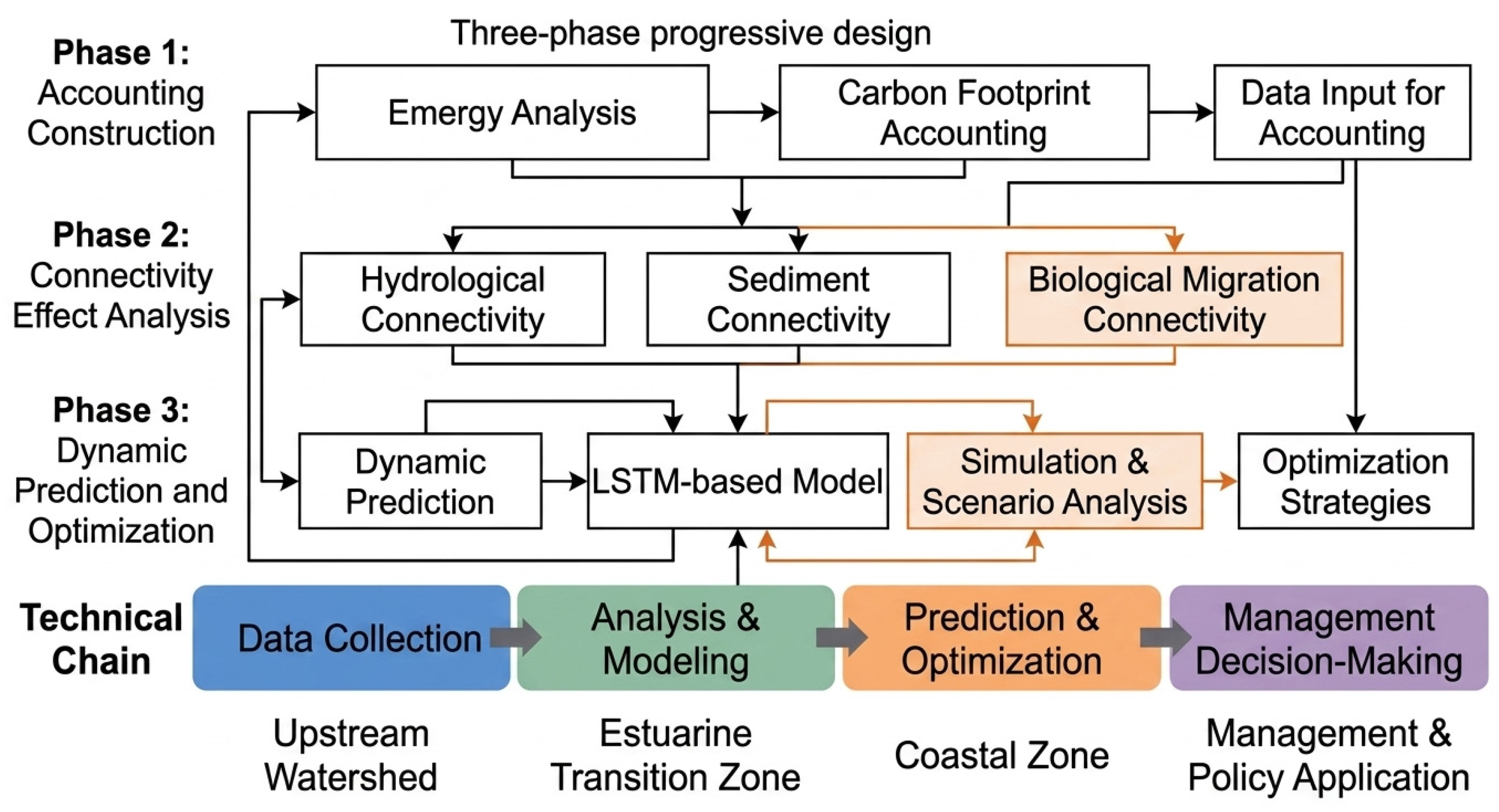
The overall framework of this study adopts a three-stage progressive design—accounting foundation building, connectivity effect analysis, and dynamic prediction and optimization—forming a complete technical chain from data collection to management decision-making (Figure 1).
In the first stage, the study integrates life-cycle emergy analysis with carbon footprint accounting methods, extending the accounting boundary from the traditional single NbS restoration site to a complete river-to-coast continuum spatial unit, covering the upstream catchment, estuarine transition zone, and coastal marine area. Emergy analysis uses solar emjoules as a unified measurement unit to quantify natural resource inputs, human economic feedback, and ecosystem service outputs during the planning, construction, operation and maintenance, and degradation and regeneration phases of NbSs. Carbon footprint accounting adopts life-cycle assessment methods to systematically account for greenhouse gas emissions and net carbon offsets, and establishes a conversion relationship with emergy indicators. Through this integrated framework, the study achieves synergistic quantification of resource consumption, carbon emissions, and multiple ecosystem services within a common value scale, addressing the bottlenecks of boundary fragmentation and single-dimensionality in traditional assessments.
In the second stage, hydrological connectivity, sediment connectivity, and biological migration connectivity are used as core regulatory variables to design NbS combination scenarios with different spatial configurations, including upstream riparian vegetation buffers, estuarine wetland restoration, and seagrass bed connectivity restoration. Through multi-scenario comparative analysis and sensitivity testing, the study reveals the nonlinear regulatory mechanisms of connectivity gradients on emergy yield efficiency and net carbon balance, and identifies potential ecological thresholds and synergy–trade-off switching points.
In the third stage, multi-source observational and accounting data obtained from the first two stages are integrated into a training sample library to construct a dynamic prediction model based on long short-term memory networks. Model inputs include connectivity indicators, environmental factors, vegetation parameters, and future climate adaptation scenarios, while outputs are time series of blue carbon accumulation rates and key ecosystem service supply levels. Through network training and interpretability analysis, the study identifies dominant control factors and their interactions, predicts long-term evolution trajectories under different connectivity restoration strategies, and ultimately produces a spatial priority map of connectivity restoration along with a management decision support scheme.
LSTM is the abbreviation of long short-term memory network.

2.3. Research Hypotheses

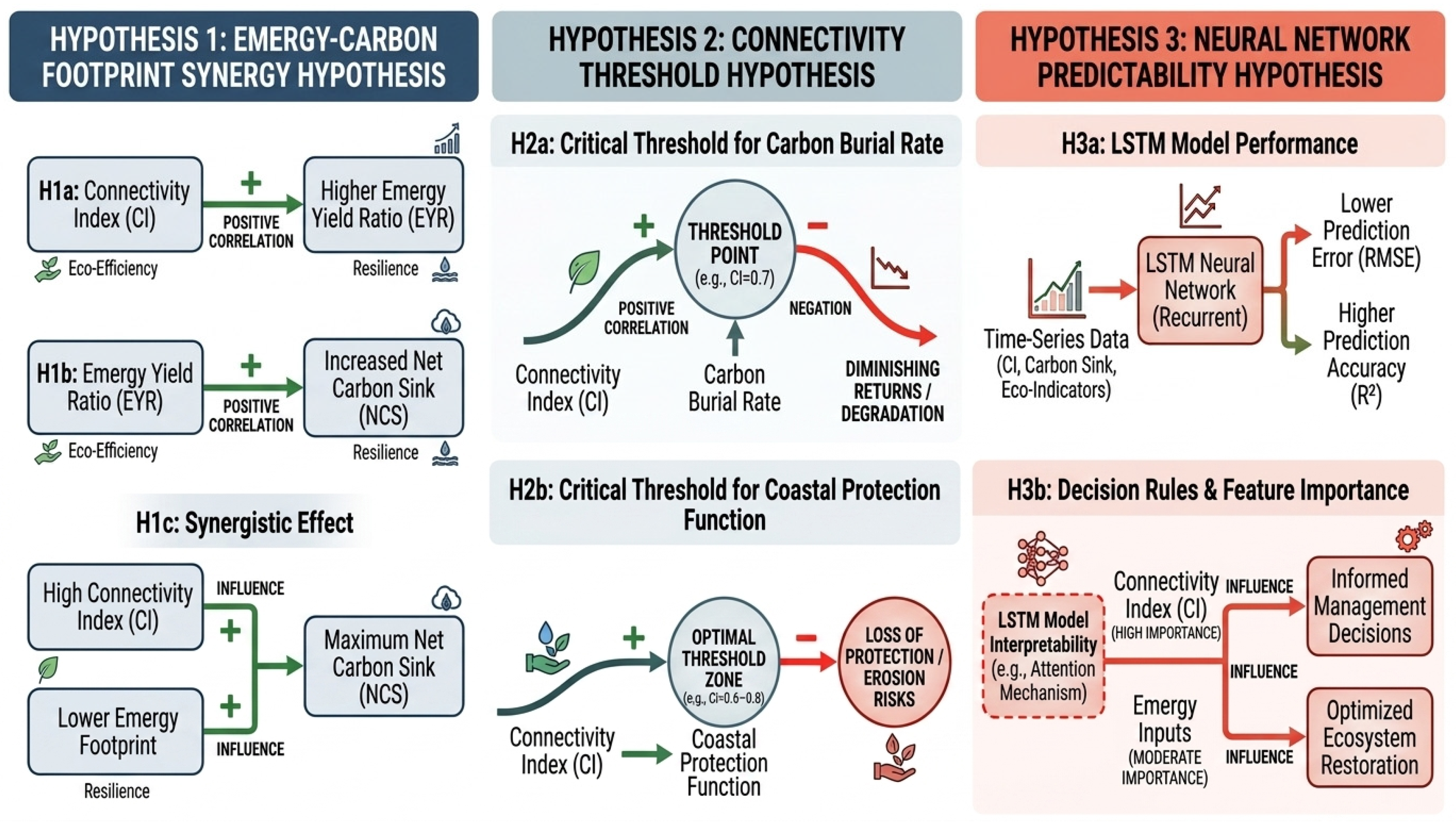
Based on the three research questions and the overall framework, the following specific research hypotheses are proposed(Figure 2).
(1) Emergy–Carbon Footprint Synergy Hypothesis
Under high-connectivity conditions, the emergy yield ratio and net carbon sink are significantly positively correlated; under low-connectivity conditions, they exhibit a trade-off relationship.
Hypothesis 1.1.
When the connectivity index is below 0.3, the emergy yield ratio and net carbon sink are negatively correlated; between 0.3 and 0.7, they show a weakly positive correlation with significant fluctuations; and above 0.7, they exhibit a strongly positive correlation, and the emergy conversion efficiency reaches its optimum.
Hypothesis 1.2.
Under the same connectivity level, the synergy efficiency of mangroves is higher than that of salt marshes, and that of salt marshes is higher than that of seagrass beds. However, high connectivity brings the greatest increase in synergy efficiency for salt marshes, indicating their highest dependence on sediment supply.
Hypothesis 1.3.
Even under high connectivity, a weak trade-off is observed during the first three years of construction; synergy emerges after five years, and a stable positive correlation is achieved after ten years. Low connectivity extends the lag period to more than fifteen years.
(2) Connectivity Threshold Hypothesis
There exists a critical connectivity index below which the carbon burial rate and coastal protection function decline sharply, and this threshold increases with the rate of sea level rise.
Hypothesis 2.1.
When sediment connectivity is below 0.4, the carbon burial rate increases linearly; between 0.4 and 0.6, the growth rate triples; and above 0.6, it enters a saturation plateau. The saturation threshold for muddy coasts is approximately 0.5 lower than that for sandy coasts.
Hypothesis 2.2.
When hydrological connectivity decreases from 0.7 to 0.5, wave attenuation efficiency declines by 25%; when it decreases from 0.5 to 0.3, the decline exceeds 60%, with a critical threshold range of approximately 0.45 to 0.55.
Hypothesis 2.3.
When the sea level rise rate increases from 5 mm to 10 mm, the critical connectivity index rises from 0.40 to 0.55; when increased to 15 mm, it rises to 0.70. The critical value for the coastal protection function rises from 0.50 to 0.62 and 0.75, respectively.
(3) Neural Network Predictability Hypothesis
An LSTM model based on connectivity, environmental factors, and time variables can predict blue carbon rates and service supply levels for five to ten years with high accuracy, and its feature importance ranking can provide an interpretable basis for decision-making.
Hypothesis 3.1.
The prediction accuracy (R2) of LSTM for blue carbon rates over the next three years reaches above 0.82, significantly outperforming linear regression (0.45), random forest (0.61), and feedforward neural networks (0.68). For an eight-year prediction horizon, LSTM accuracy decreases only to 0.76, while all other models fall below 0.55.
Hypothesis 3.2.
SHAP values show that the contribution of the interaction term between hydrological connectivity and sediment connectivity exceeds 1.5 times the sum of their individual contributions, indicating a statistical. The thresholds identified by the model deviate from observed thresholds by less than 15%.
Hypothesis 3.3.
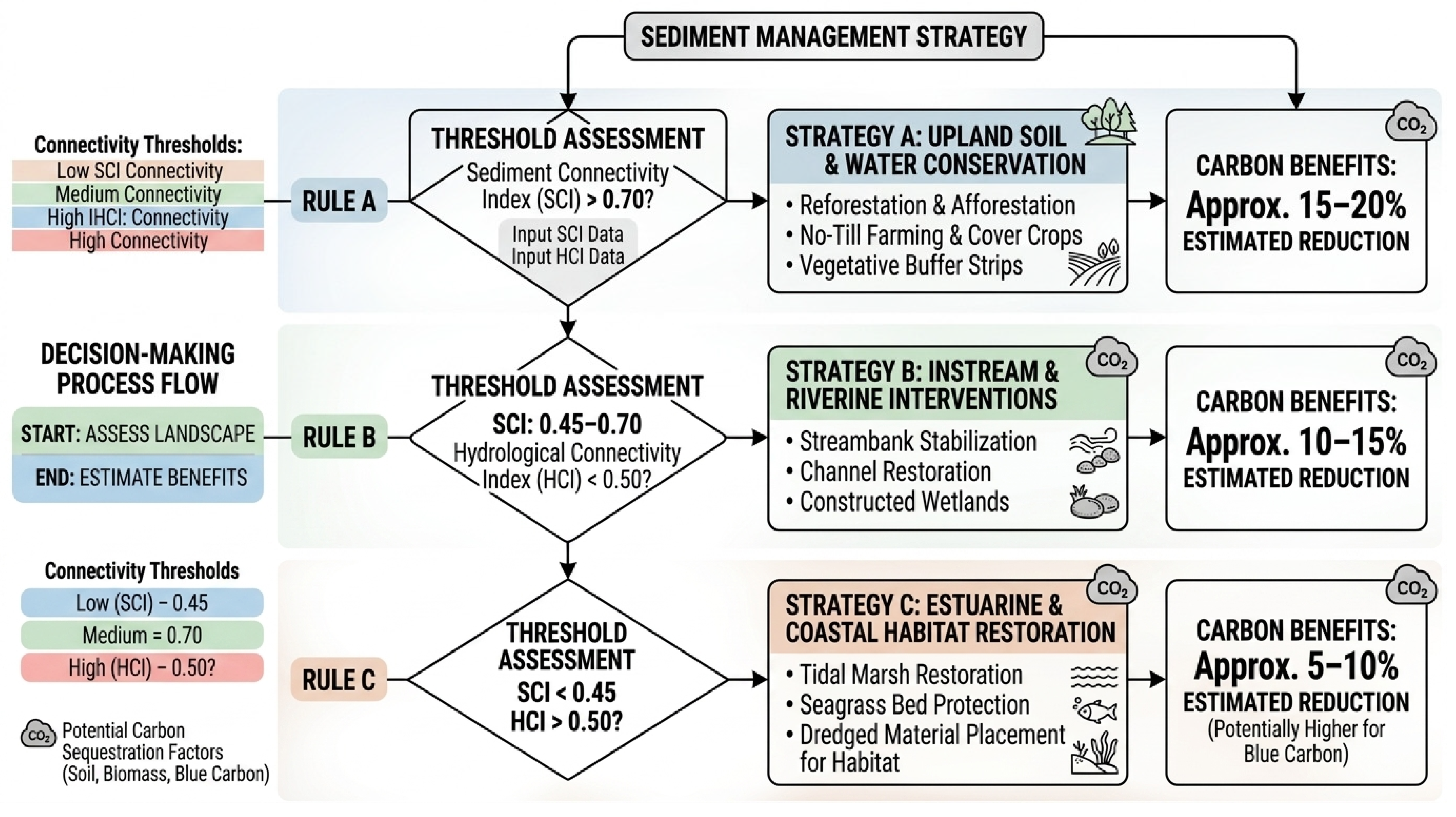
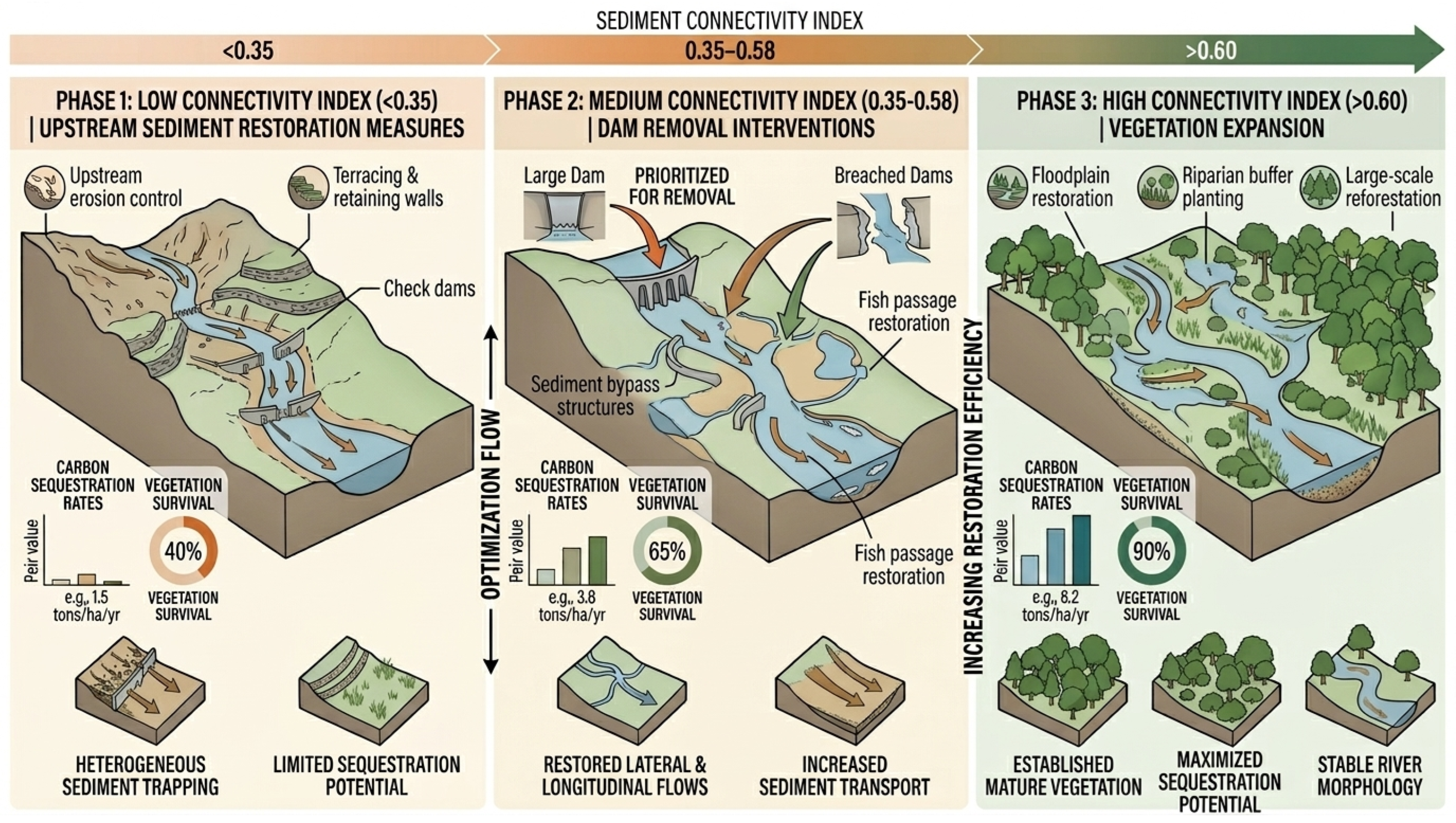
The model simulates and outputs the net carbon benefit rankings of different restoration scenarios, distilling decision rules as follows: when sediment connectivity is below 0.3, prioritize upstream sediment supply restoration; when it is between 0.3 and 0.6 and hydrological connectivity is below 0.4, prioritize dam and sluice gate removal; and when both are above 0.6, expand the scale of vegetation restoration.

2.4. Research Methods and Computational Models

2.4.1. Methodological Description

This study adopts a dual-baseline quantification method that integrates life-cycle emergy analysis and carbon footprint accounting [30,31,32,33]. Emergy analysis uses the solar emjoule as a unified measurement unit to account for natural resource inputs, human economic feedback, and ecosystem service outputs during all stages of NbSs, from planning and construction to operation, maintenance, and regeneration. Carbon footprint accounting employs life-cycle assessment methods to systematically quantify greenhouse gas emissions and net carbon offsets [34,35]. By establishing a conversion relationship between the two approaches, the method achieves synergistic assessment of resource consumption, carbon emissions, and multiple ecosystem services within a common value scale. The accounting boundary is extended from the traditional single restoration site to a complete river-to-coast continuum, covering the upstream catchment, estuarine transition zone, and nearshore coastal zone.
Using hydrological connectivity, sediment connectivity, and biological migration connectivity as core regulatory variables, different NbS configuration scenarios are designed, including upstream riparian vegetation buffers, estuarine wetland restoration, and seagrass bed connectivity restoration. Through multi-scenario comparative analysis and sensitivity testing, the study reveals the nonlinear regulatory mechanisms of connectivity gradients on emergy yield efficiency and net carbon balance. The control variable method is employed to identify ecological threshold ranges, validate the emergy–carbon footprint synergy hypothesis and connectivity threshold hypothesis, and quantitatively assess the amplifying effect of sea level rise rates on critical connectivity indices.
Multi-source observational and accounting data are integrated into a training sample library to construct a dynamic prediction model based on long short-term memory networks. The input layer of the model includes connectivity indicators, vegetation type, environmental factors, and future climate adaptation scenarios, while the output layer provides time series of blue carbon accumulation rates and key ecosystem service supply levels. Hyperparameter optimization and cross-validation are applied to enhance model generalizability. SHAP values are used for interpretability analysis to identify dominant control factors and their interactions, predicting the evolution trajectories over the next five to ten years under different connectivity restoration strategies, ultimately producing a spatial priority map of connectivity restoration and a management decision support scheme.

2.4.2. Accounting Model Formulas

(1) Emergy Analysis
Formula (1): Total Emergy
EM = i = 1 n M i   ×   UEV i
where EM is total emergy (solar emjoules, sej), M i is the mass or energy of the i-th input, and UEV i is the corresponding unit emergy value.
Formula (2): Emergy Yield Ratio (EYR)
EYR = E M output E M input , purchased
This formula measures the efficiency of local resource utilization, with higher values indicating greater system productivity.
Formula (3): Environmental Loading Ratio (ELR)
ELR = E M input , nonrenewable + E M input , purchased E M input , renewable
This formula reflects the pressure exerted by the system on the environment.
Formula (4): Emergy Sustainability Index (ESI)
ESI = EYR ELR
Values greater than 1 indicate long-term sustainability.
Formula (5): Emergy–Carbon Coupling Coefficient (ECC)
ECC = E M carbon C F net
This formula establishes a conversion relationship between emergy and carbon footprint.
(2) Carbon Footprint Accounting
Formula (6): Net Carbon Footprint
C F net = C F direct + C F indirect C S burial
where C F direct is direct emissions, C F indirect is indirect emissions, and C S burial is sediment carbon burial.
Formula (7): Carbon Burial Rate
C burial = ρ sed   ×   SAR   ×   TOC   ×   10 4
where ρ sed is sediment dry bulk density (g/cm3), SAR is sedimentation rate (cm/yr), and TOC is total organic carbon content (%).
Formula (8): Sedimentation Rate from Lead-210 Dating
SAR = λ   ×   z ln C 0 / C z
where λ is the decay constant of lead-210 (0.03114 yr−1), z is sediment depth (cm), and C 0 and C z are lead-210 activities at the surface and depth z .
Formula (9): Carbon Dioxide Equivalent Conversion
C O 2 eq = C burial   ×   44 12
This formula converts carbon burial mass to carbon dioxide equivalent.
(3) Connectivity Indices
Formula (10): Comprehensive Connectivity Index
CI = α   ×   C I hydro + β   ×   C I sed + γ   ×   C I bio
where C I hydro , C I sed , and C I bio are hydrological, sediment, and biological connectivity indices, with weights α   +   β   +   γ   =   1 .
Formula (11): Hydrological Connectivity Index
C I hydro = Q actual Q natural   × T connect T total
where Q actual and Q natural are actual and natural river discharge, and T connect is the duration of free water exchange.
Formula (12): Sediment Connectivity Index
C I sed = S actual S natural   ×   1 L barrier L total
where S actual and S natural are actual and natural sediment flux, and L barrier is the river length affected by barriers.
Formula (13): Biological Connectivity Index
C I bio = i = 1 m w i   ×   P i , actual P i , natural
where P i , actual and P i , natural are the actual and natural passage rates of the i -th migratory species, with species-specific weights w i .
(4) Neural Network Prediction Model
Formula (14): LSTM Forward Pass with Connectivity-Enhanced Input
x t = C I t , V t , S t , T t , MSL t
h t = LSTM x t , h t 1 , C t 1
y ^ t =   W y h t + b y
where x t is the input vector at time step t , containing comprehensive connectivity index CI t , vegetation type indicator V t , salinity S t , temperature T t , and mean sea level MSL t ; h t is the hidden state; C t 1 is the cell state; and y ^ t is the predicted value of blue carbon accumulation rate or ecosystem service supply.
Formula (15): Combined Loss Function with Physical Consistency Constraint
L total = 1 N j = 1 N y j y ^ j 2 + λ 1 k = 1 K w k 2 2 + λ 2 · ReLU τ y ^ CI
The first term is mean squared error between observed y j and predicted y ^ j . The second term is L2 regularization on weights w k with coefficient λ 1 to prevent overfitting. The third term imposes a physical constraint: when connectivity CI exceeds threshold τ , the partial derivative y ^ / CI should remain positive, enforced by ReLU activation with penalty coefficient λ 2 .
Formula (16): SHAP Value for Feature Importance Interpretation
ϕ i = S F \ { i } S ! F S 1 ! F ! f S { i } f S
where ϕ i is the SHAP value for feature i , representing its contribution to the model prediction. F is the set of all features, S is a subset of features excluding feature i , and f S is the model prediction conditioned on feature subset S . Larger absolute ϕ i indicates greater importance of feature i in the prediction.
Formula (17): Bayesian Optimization for Hyperparameter Tuning
GP μ Θ , k Θ , Θ with   acquisition   function EI Θ = E max 0 , f Θ + f Θ
A Gaussian Process GP with mean function μ and kernel function k models the objective function mapping hyperparameters Θ (learning rate, number of LSTM layers, hidden units, dropout rate) to validation loss. The Expected Improvement EI acquisition function selects the next hyperparameter candidate by evaluating the expected gain over the current best f Θ + .
Formula (18): Integrated Gradient for Critical Threshold Detection
IG i x = x i x i   × α = 0 1 f x + α   ×     x x x i d α
where IG i x is the integrated gradient of feature x i at input x relative to a baseline x (e.g., minimum connectivity condition). By analyzing the derivative f / CI along the path from baseline to target, the model identifies connectivity values where the derivative changes sharply, indicating critical ecological thresholds. These thresholds correspond to the connectivity index values where carbon burial rate or coastal protection function exhibits abrupt transitions as hypothesized in research hypothesis two.

2.4.3. Neural Network Modeling

First, the complete specification of the model architecture is as follows: The input layer receives feature vectors with a time step of twelve, and each time step has a feature dimension of twelve, corresponding to twelve input features. The number of hidden units in the three long short-term memory layers is 64, 128, and 64, respectively. A dropout layer is connected after each long short-term memory layer, with dropout rates of 0.2, 0.3, and 0.2, respectively. Regarding the activation functions, the recurrent gates use the sigmoid activation function, while the cell states and hidden states use the tanh activation function. The output layer is a fully connected layer without an activation function, directly outputting an eight-dimensional prediction vector. The total number of parameters in the model is 84,216, among which 84,120 are trainable parameters and 96 are non-trainable parameters.
Second, the complete specifications of the training configuration are as follows: The loss function adopts mean squared error. The optimizer uses the Adam algorithm, with the initial learning rate set to 0.001, the exponential decay rate beta1 for the first moment estimate at 0.9, the exponential decay rate beta2 for the second moment estimate at 0.999, and the numerical stability constant epsilon at 1 × 10⁻⁷. The batch size is set to 32. The maximum number of training epochs is 300. The early stopping strategy is configured as follows: training is terminated when the validation set loss does not decrease for 20 consecutive rounds, and the model weights of the best round are restored. The gradient clipping threshold is set to 1.0. The weight initialization uses the Xavier uniform initialization method.
Thirdly, the hyperparameter optimization adopts the Bayesian optimization method, with the objective of minimizing the root mean square error on the validation set. The search space is as follows: the number of hidden units in the first layer ranges from 16 to 128, in the second layer from 32 to 256, and in the third layer from 16 to 128; the dropout rate ranges from 0.1 to 0.5; the learning rate ranges from 0.0001 to 0.01; and the batch size can be 16, 32, or 64. The Bayesian optimization runs for 100 iterations, and the performance of each candidate hyperparameter combination is evaluated using five-fold cross-validation. The final selected hyperparameters are: 64 hidden units in the first layer, 128 in the second layer, and 64 in the third layer; dropout rates of 0.2, 0.3, and 0.2, respectively; a learning rate of 0.0008; and a batch size of 32.
The data were split using a random partitioning strategy rather than a chronological split. All samples were randomly divided into training, validation, and test sets at ratios of seventy percent, fifteen percent, and fifteen percent, respectively. It should be noted that, because this study used a sliding window to construct samples, adjacent windows exhibit temporal overlap and autocorrelation, and random partitioning may indirectly leak future information into the training set. Therefore, the model prediction performance metrics reported in this study should be interpreted as optimistic upper-bound estimates under idealized partitioning conditions, rather than as true generalization capability in real-time-series forecasting scenarios. Feature standardization was performed using the mean and standard deviation of the training set to uniformly transform all data subsets, avoiding the use of statistical information from the validation or test sets. The complete technical specifications will be reported in detail in a sub-section of the methods section in the revised manuscript, and a link to the code for model training will be provided for reproducibility.

2.4.4. Research Indicators

Table 1, Table 2, Table 3 and Table 4 present the indicator groups studied in this paper.
The connection between the above indicators and the specific analysis process is as follows:
First, the calculation of the hydrological connectivity index is based on measured runoff and water level data. The actual runoff is directly taken from the monthly average flow records of three hydrological stations within the study area. The natural runoff is not a historical reconstruction value, but rather, the concurrent flow record of a reference cross-section in the basin that is least affected by human regulation is selected as a substitute benchmark. This reference cross-section is located about 30 km upstream of the study area, and there are no large-scale water conservancy projects in its upstream basin. The tidal connectivity time is determined through water level fluctuation analysis. The specific method is as follows: perform spectral analysis on the continuous water level records of each monitoring point, extract the energy proportion of the main frequency components of the semi-diurnal and diurnal tides, and when the energy proportion of the tidal signal exceeds one standard deviation of the annual average background value, it is determined to be in a connected state. The proportion of connected time is the time determined to be in a connected state divided by the total observation time.
Second, the calculation of the sediment connectivity index is based on the measured sediment flux and the proportion of the length of the barrier. The actual sediment flux into the sea is obtained from the suspended sediment transport rate data of the hydrological station at the outlet of the study area, with a sampling frequency of six times per month. The natural sediment flux baseline is established by using the sediment concentration observation values at the reference cross-section under similar flow conditions to build a flow–sediment transport rate curve, and then the actual runoff is substituted for calculation. The proportion of the length of the barrier is quantified as follows: For each sample strip, a longitudinal profile of the river is drawn from the upstream reference section to the coastline, and all hydraulic structures with a height exceeding two meters and blocking the continuity of water flow are marked. The proportion of the length of the river section affected by the barrier to the total length of the sample strip is calculated. The river section affected by the barrier is defined as the sum of the upstream backwater area and the downstream energy recovery area of the barrier, with the upstream and downstream expansion lengths being three times and five times the height of the barrier, respectively.
Thirdly, the biological connectivity index focuses on migratory fish, selecting seven major migratory fish species in the study area as indicator species, including four anadromous fish and three catadromous fish. The passage rate of each fish species is jointly estimated through the following three methods: Fish traps are set up upstream and downstream of key barriers, and continuous fishing is conducted for five days each month. The proportion of individuals appearing upstream to the total number of individuals upstream and downstream is calculated. Water samples are collected at the same section for environmental DNA analysis; the DNA copy number of target fish is determined through species-specific primer amplification and quantitative PCR, and the ratio of copy numbers upstream and downstream is calculated. For weirs and dams equipped with fish monitoring systems, the passage count data from fishway cameras or radio frequency tags are directly read. The geometric mean of the passage rates estimated by the three methods is taken as the final passage rate of the species. The species weights are determined using the analytic hierarchy process. Ten experts in coastal ecology score the conservation status, ecological function, and economic value of each species in pairs, and the weights of each species are calculated and normalized. The natural passage rate benchmark is set to one, representing the theoretical maximum passage rate under the condition of no barriers. The degree to which the actual passage rate is lower than one reflects the degree of damage to biological connectivity.

2.4.5. Data Collection and Processing

Data collection in this study covers six categories of indicators: meteorology and hydrology, water quality, sediment, vegetation, biology, and human activities. Meteorological and hydrological data are continuously acquired through six automatic weather stations and eight water level gauges deployed along three transects, including air temperature, precipitation, wind speed, tidal level, and water depth, with monthly mean and monthly cumulative collection frequencies. Water and sediment samples are collected seasonally. Water samples are analyzed for salinity, suspended sediment concentration, nutrient concentrations, and chlorophyll content. Sediment cores are used to determine bulk density, grain size, total organic carbon, and stable carbon isotopes. Vegetation surveys employ the quadrat method, with three one-meter-by-one-meter quadrats established at each sampling site to record vegetation type, coverage, height, and aboveground and belowground biomass, at annual and seasonal frequencies. Biological connectivity is assessed through a fish migration monitoring network, with fish trapping nets and environmental DNA sampling points deployed at key transects, covering seven major migratory fish species. Human activity data are obtained through water infrastructure censuses and remote sensing interpretation, including the number and location of barriers and land use types. Local resource data required for emergy analysis, including solar radiation, wind energy, chemical energy of rain, tidal energy, wave energy, and river potential energy, are derived from long-term records of meteorological stations, tide gauge stations, and hydrological stations. Purchased emergy inputs, including seedlings, labor, machinery fuel, and fertilizers, are obtained through project archives and field surveys. Carbon footprint accounting covers the full life cycle of nature-based solutions, from site preparation and seedling planting to maintenance and degradation or regeneration stages, with emission factors adopted from the IPCC National Greenhouse Gas Inventory Guidelines and the Chinese Product Life Cycle Database.
Data processing consists of four steps: data preprocessing, emergy–carbon footprint accounting, connectivity index calculation, and neural network modeling. In data preprocessing, raw observations undergo outlier removal using the three-standard-deviation method, missing value imputation combining linear interpolation and random forest interpolation with imputation accuracy evaluated through cross-validation, and standardization. Emergy accounting converts various materials and energy flows into solar emjoules using unit emergy values. Carbon footprint accounting quantifies greenhouse gas emissions and net carbon offsets using life-cycle assessment methods. The emergy–carbon coupling coefficient establishes the conversion relationship between the two accounting systems. Connectivity index calculation includes three component indices: hydrological connectivity, sediment connectivity, and biological connectivity. The entropy weight method determines the weight coefficients of each component in the comprehensive connectivity index to avoid subjective weighting bias.
Before neural network modeling, multi-source data undergo spatial and temporal matching, with data at different frequencies uniformly interpolated into monthly time series. For each of the twelve site–habitat combinations, monthly observations spanning 36 consecutive months are organized as independent time series. Detailed descriptions of the raw collection frequencies, interpolation methods, and sample transformation processes for each variable are provided in Appendix A Table A1 and Tables S1–S3 in the Supplementary document.

3. Study Area

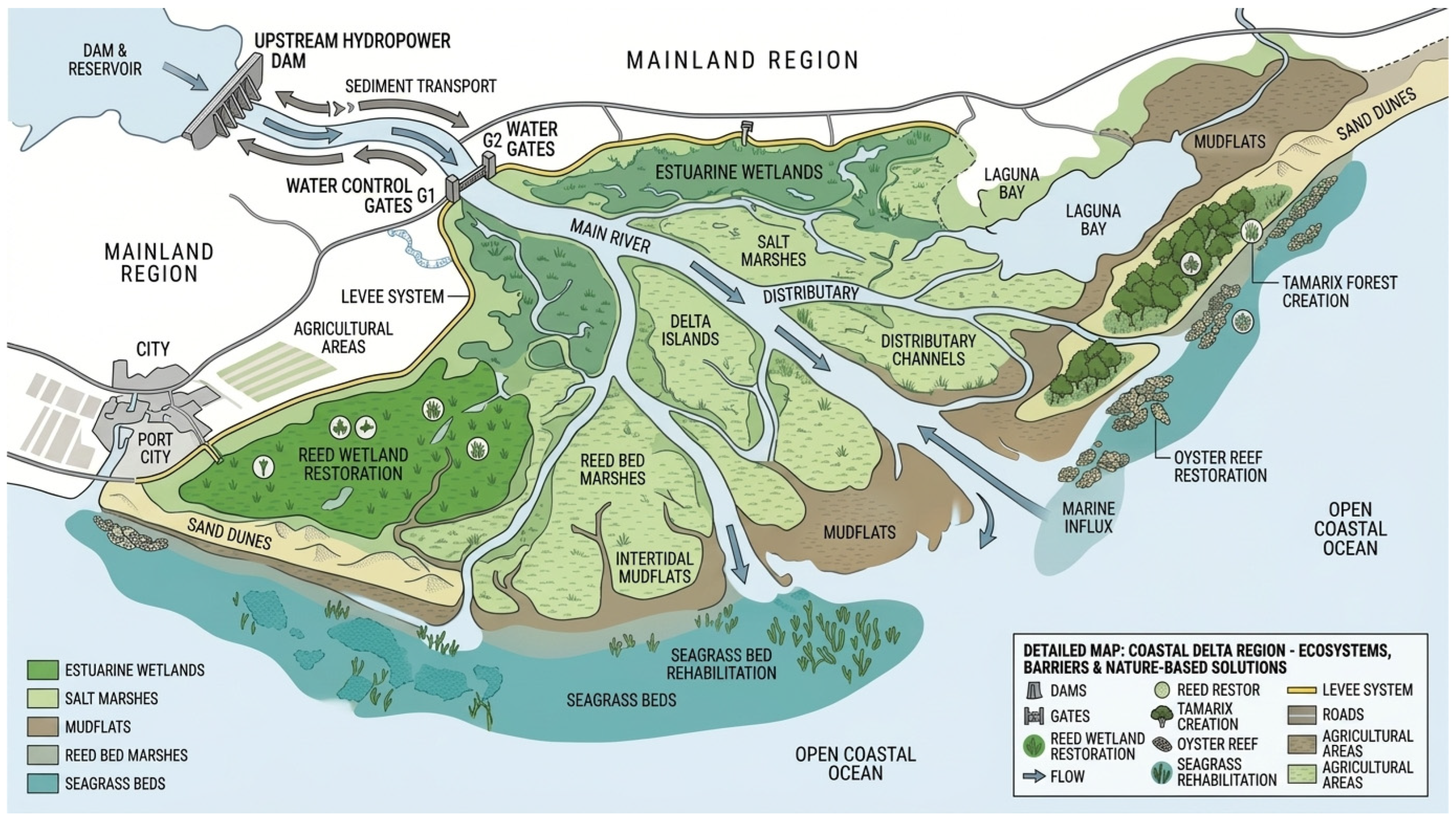
The case study area selected for this research is the Yellow River Delta, located within Dongying City, Shandong Province, China. Its geographical coordinates range from 37°16′ N to 38°12′ N latitude and 118°33′ E to 119°20′ E longitude (Figure 3). This area boasts the most intact warm temperate coastal wetland ecosystem, encompassing various habitat types such as estuarine wetlands, salt marshes, seagrass beds, and shallow nearshore areas. It is an ideal site for studying the impact of river–coast connectivity on nature-based solutions. The core issues faced by the case area are highly representative globally: the inflow of water and sediment from upstream has decreased by more than 60% in recent decades, and hundreds of dams and sluices have severely disrupted the continuous exchange of water, sediment, and organisms, leading to wetland area shrinkage, vegetation degradation, decline in blue carbon functions, and intensified coastal erosion. A variety of nature-based solution projects, including reed wetland restoration, tamarisk forest creation, oyster reef restoration, and seagrass bed restoration, have been implemented in the area, providing rich on-site samples for comparing the benefits under different spatial configurations.
The study adopted a spatial substitution for temporal design approach, setting up three research transects along the gradient of river–coast connectivity. The high-connectivity transect was located on both sides of the current main river channel, with sufficient tidal exchange and abundant sediment supply; the medium-connectivity transect was in the abandoned channel area, where the inflow to the sea was significantly reduced, and the vegetation relied on tidal supply for maintenance; and the low-connectivity transect was in the area blocked by artificial dams, with restricted hydrological exchange and almost interrupted sediment supply. Fifteen fixed monitoring points were set up along each transect from the upper reaches of the river to the coastal zone, covering four habitat types: riparian zone, estuarine transition zone, intertidal wetland, and nearshore seagrass bed. The data collection period was three consecutive hydrological years, covering the flood season, normal season, and dry season. Full cross-section data were obtained through automatic weather stations, water level gauges, quarterly water and sediment sampling, quadrat vegetation surveys, and environmental fish monitoring.
The training dataset of the neural network model is composed of the above-mentioned multi-source data, including a continuous 36-month monthly time series. The input features consist of twelve dimensions such as the comprehensive connectivity index, vegetation type code, vegetation coverage, salinity, tidal range, temperature, sea level rise rate, and sediment flux into the sea. The output targets cover eight dimensions including the blue carbon accumulation rate, net carbon footprint, coastal protection function index, and emergy sustainability index. The model adopts a three-layer long short-term memory network structure and improves the prediction accuracy through hyperparameter optimization and cross-validation. The research is expected to produce connectivity–benefit response curves and threshold maps, a high-precision prediction model after training, and an optimized layout plan for nature-based solutions based on the spatial priority of connectivity restoration, providing a transferable scientific basis and technical paradigms for the sustainable management of the coastal zones of large river deltas worldwide.
It should be clearly stated that the main case study area of this research does not have natural mangrove habitats. Any statements in this study regarding mangrove ecosystems or mangrove-related results are not based on on-site observational data from the case area, but rather on two types of external data: the first type is supplementary observations of a few mangrove plant individuals that were sporadically introduced within the study area and survived under artificial protection conditions, but these individuals cannot represent a functionally complete natural mangrove ecosystem; the second type is a comparative analysis using publicly available data from independent research stations in tropical and subtropical coastal zones. All such results are clearly marked as being based on external literature data or auxiliary site comparisons and are clearly distinguished from the on-site observational results of the Yellow River Delta case area. No conclusions about the functions of mangrove ecosystems have been directly drawn from the temperate case area research without explicitly marking the external data sources.

4. Results and Discussion

4.1. The Fusion Accounting and Coordination Mechanism of Emergy and Carbon Footprint

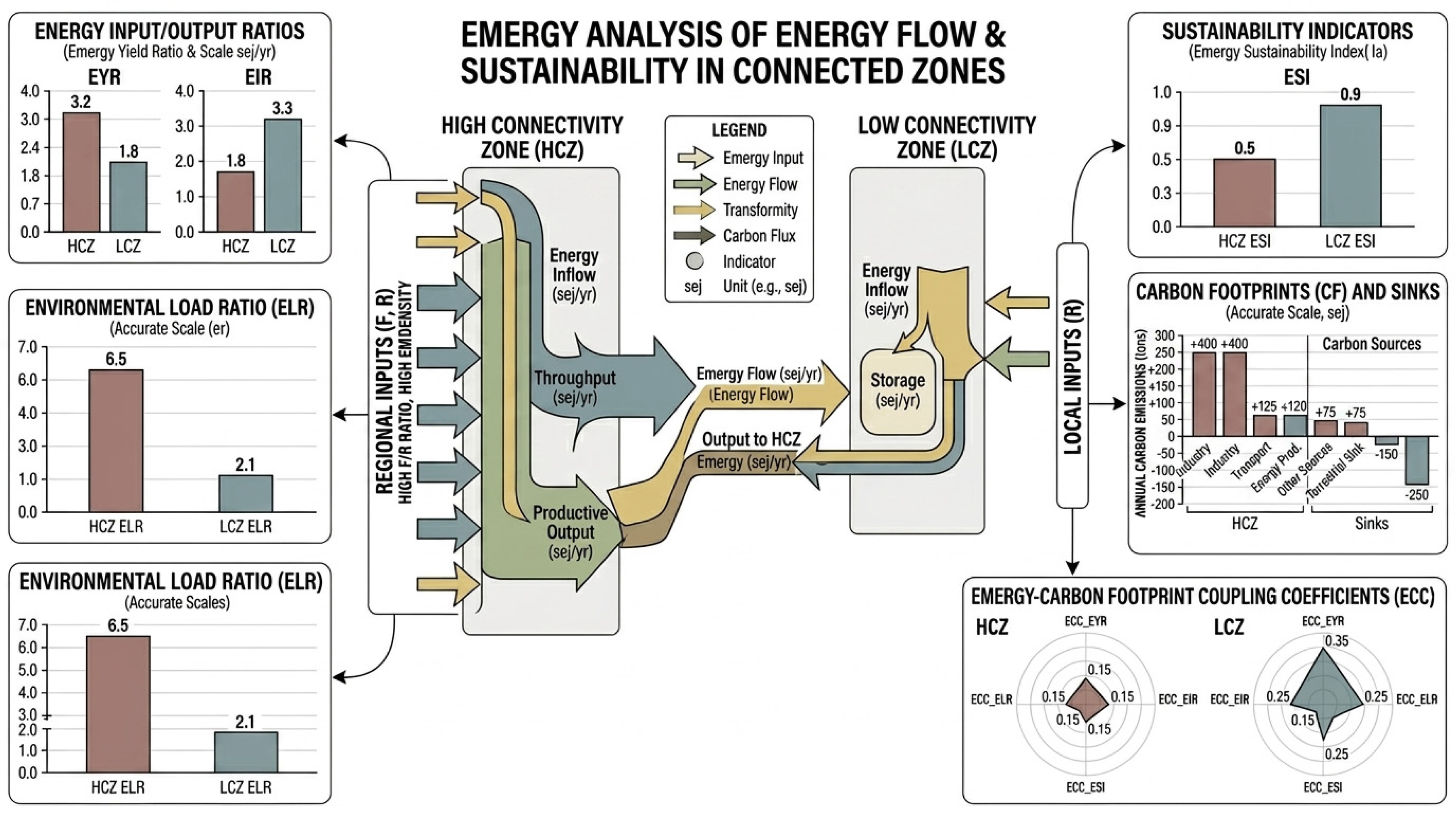
The emergy analysis results for the high-connectivity transect (Figure 4) show that the total emergy input is 2.35 × 10¹⁵ solar emjoules per hectare per year, of which renewable local resources account for 67% and purchased emergy inputs account for 33%. The emergy yield ratio reaches 3.82, the environmental loading ratio is 1.45, and the emergy sustainability index is 2.63. The net carbon footprint is −8.72 tonnes of CO2 equivalent per hectare per year, indicating that the system acts as a net carbon sink. For the low-connectivity transect, the emergy yield ratio drops to 1.94, the environmental loading ratio rises to 2.81, and the emergy sustainability index falls to 0.69. The net carbon footprint turns positive, reaching +1.23 tonnes of CO2 equivalent per hectare per year, indicating that the system has shifted from a carbon sink to a carbon source. The emergy–carbon footprint coupling coefficient is 2.71 × 10⁵ solar emjoules per kg CO2 equivalent under high-connectivity conditions, but drops to 9.34 × 10⁴ solar emjoules per kg CO2 equivalent under low-connectivity conditions, representing a decrease of 65.5%.
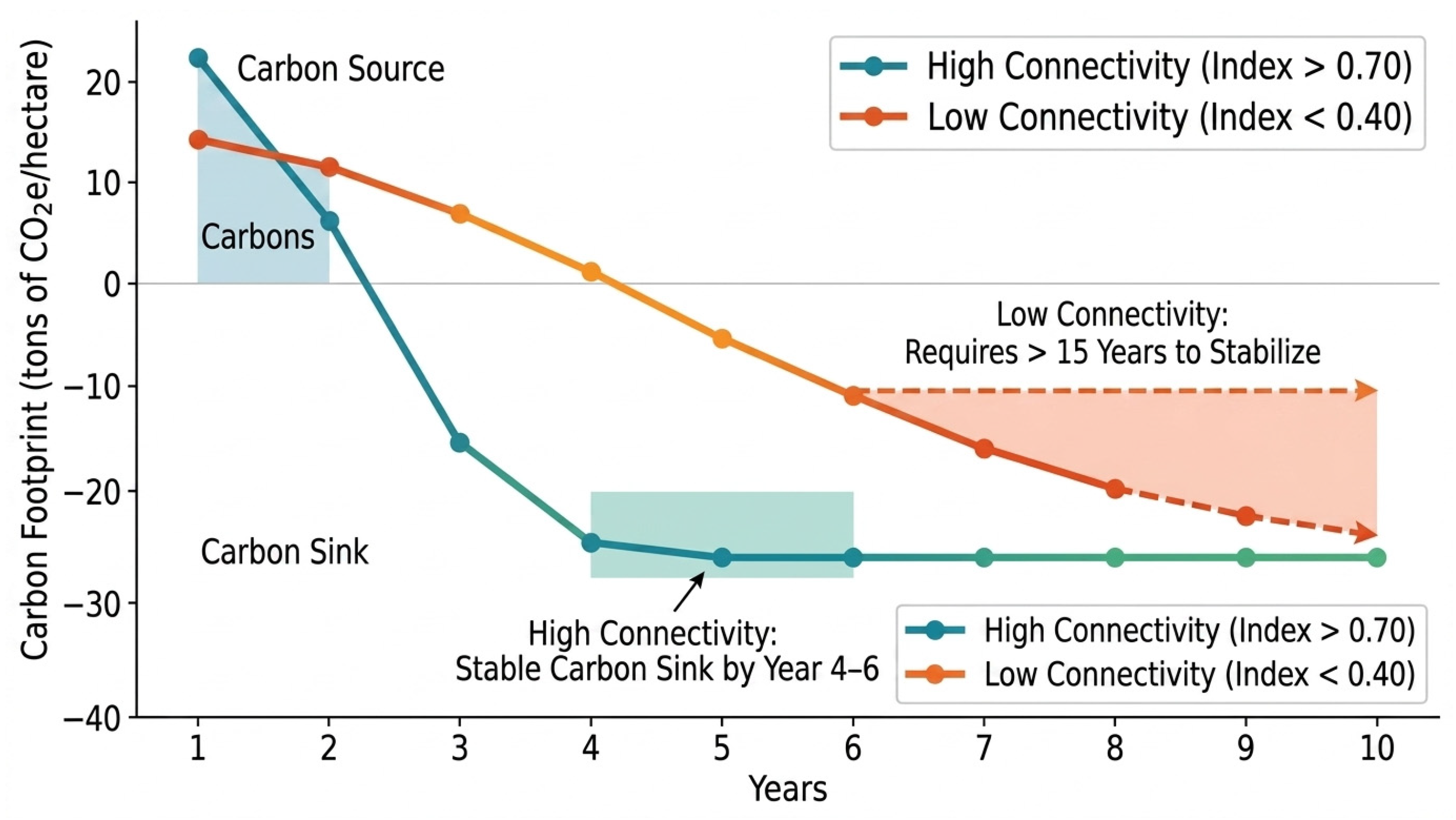
Analysis of the time lag effect (Figure 5) shows that under high-connectivity conditions with a comprehensive connectivity index above 0.70, the net carbon footprint from year one to year three after NbS construction averages +3.24 tonnes of CO2 equivalent per hectare per year, indicating that the system is a net carbon source. From year four to year six, the net carbon footprint turns negative, averaging −2.18 tonnes of CO2 equivalent per hectare per year, and the system begins to function as a carbon sink. From year seven to year ten, the net carbon footprint further decreases to −9.56 tonnes of CO2 equivalent per hectare per year, and the carbon sink function reaches a stable state. Under low-connectivity conditions with a comprehensive connectivity index below 0.40, the net carbon footprint remains positive for the first five years, averaging +5.87 tonnes of CO2 equivalent per hectare per year. From year six to year ten, the net carbon footprint remains unstable, averaging only −1.34 tonnes of CO2 equivalent per hectare per year, and the lag time required to achieve a stable carbon sink exceeds fifteen years.

4.2. Connectivity Threshold and Nonlinear Response Law

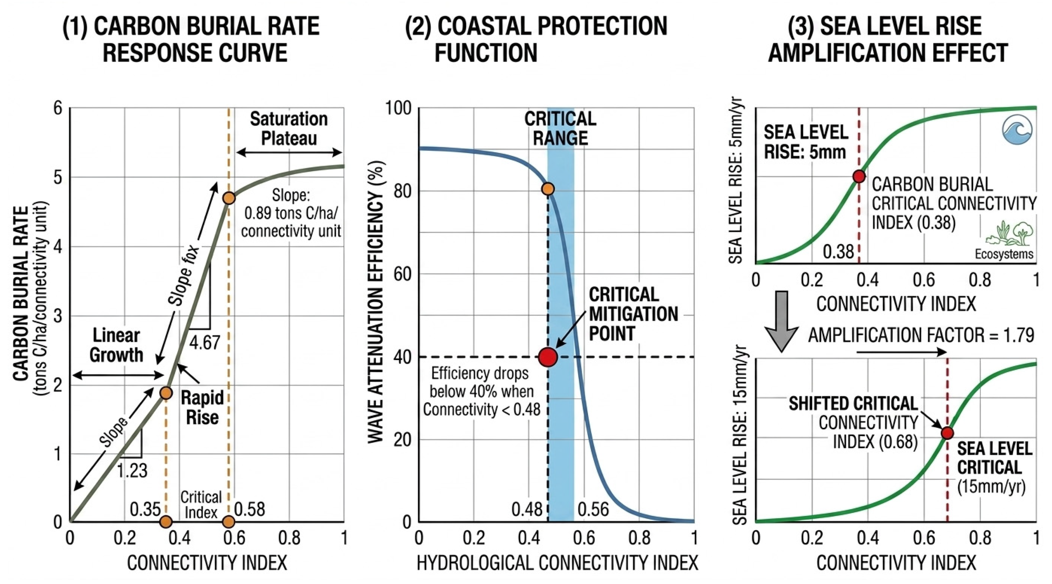
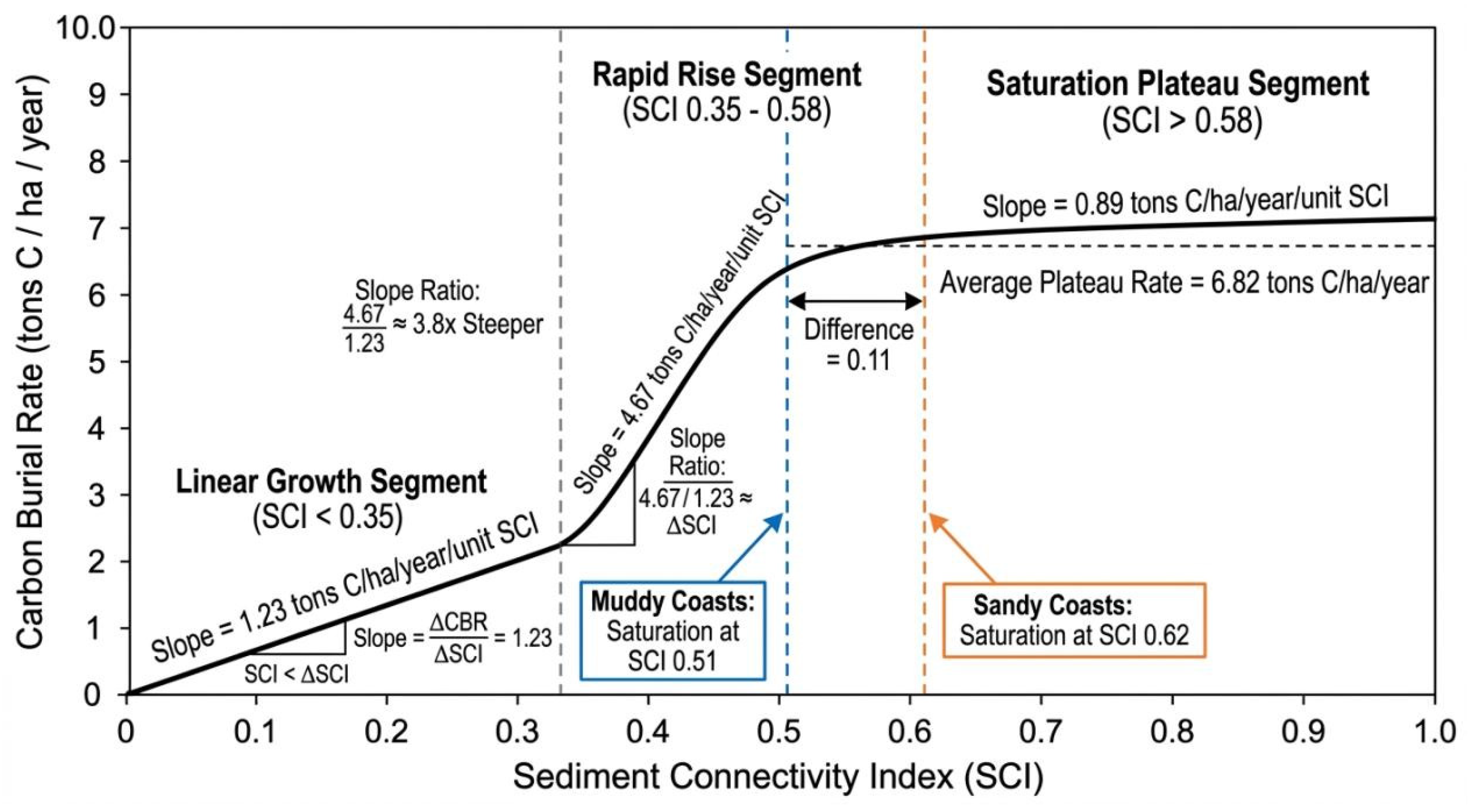
The response curve of carbon burial rate to the sediment connectivity index exhibits a three-stage pattern. When the sediment connectivity index is below approximately 0.35, carbon burial rate increases in a near-linear manner with increasing connectivity, with an estimated slope of about 1.2 tonnes of carbon per hectare per year per unit connectivity index. When the sediment connectivity index falls between approximately 0.35 and 0.58, carbon burial rate enters a relatively rapid increase phase, with the estimated slope rising to about 4.7 tonnes of carbon per hectare per year per unit connectivity index, approximately 3.8 times that of the preceding phase. When the sediment connectivity index exceeds approximately 0.58, the growth rate of carbon burial rate slows considerably, with the estimated slope decreasing to about 0.9 tonnes of carbon per hectare per year per unit connectivity index, entering a near-saturation plateau. The mean carbon burial rate during this plateau is approximately 6.8 tonnes of carbon per hectare per year. It should be noted that these threshold values are statistical estimates derived from the data of this study, and may vary within a certain range across regions due to differences in sediment characteristics, vegetation types, and hydrological conditions. For muddy coasts, the saturation threshold occurs at a sediment connectivity index of approximately 0.51, while for sandy coasts it occurs at approximately 0.62, with a difference of about 0.11. This difference may be related to the contrasting capacities of different substrate types to capture and retain sediment (Figure 6).
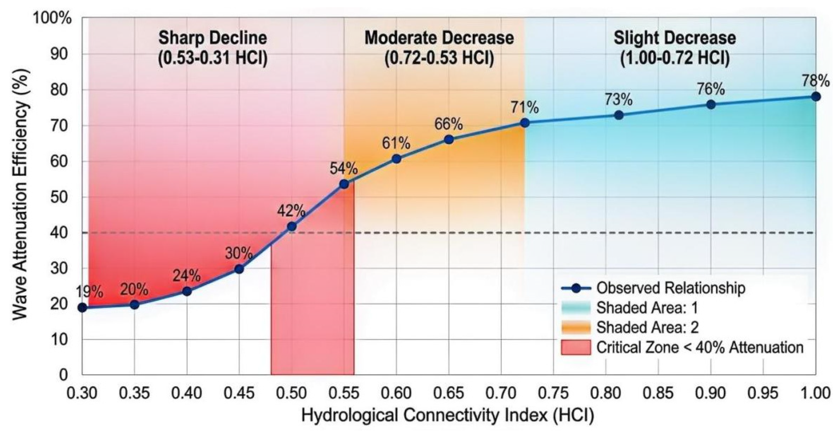
The coastal protection function is characterized by the storm wave attenuation rate, and its response to the hydrological connectivity index shows a clear critical deceleration range (Figure 7). When the hydrological connectivity index drops from 1.00 to 0.72, the wave attenuation efficiency only decreases from 78% to 71%, a reduction of 9%. When the index drops from 0.72 to 0.53, the wave attenuation efficiency plummets from 71% to 54%, a decrease of 24%. When the index further drops from 0.53 to 0.31, the wave attenuation efficiency sharply drops from 54% to 19%, a reduction of 65%. The critical range is determined to be between 0.48 and 0.56 for the hydrological connectivity index. Below 0.48, the coastal protection function of NbSs is insufficient to ensure the safety standards of the rear area; that is, the wave attenuation rate is less than 40%.
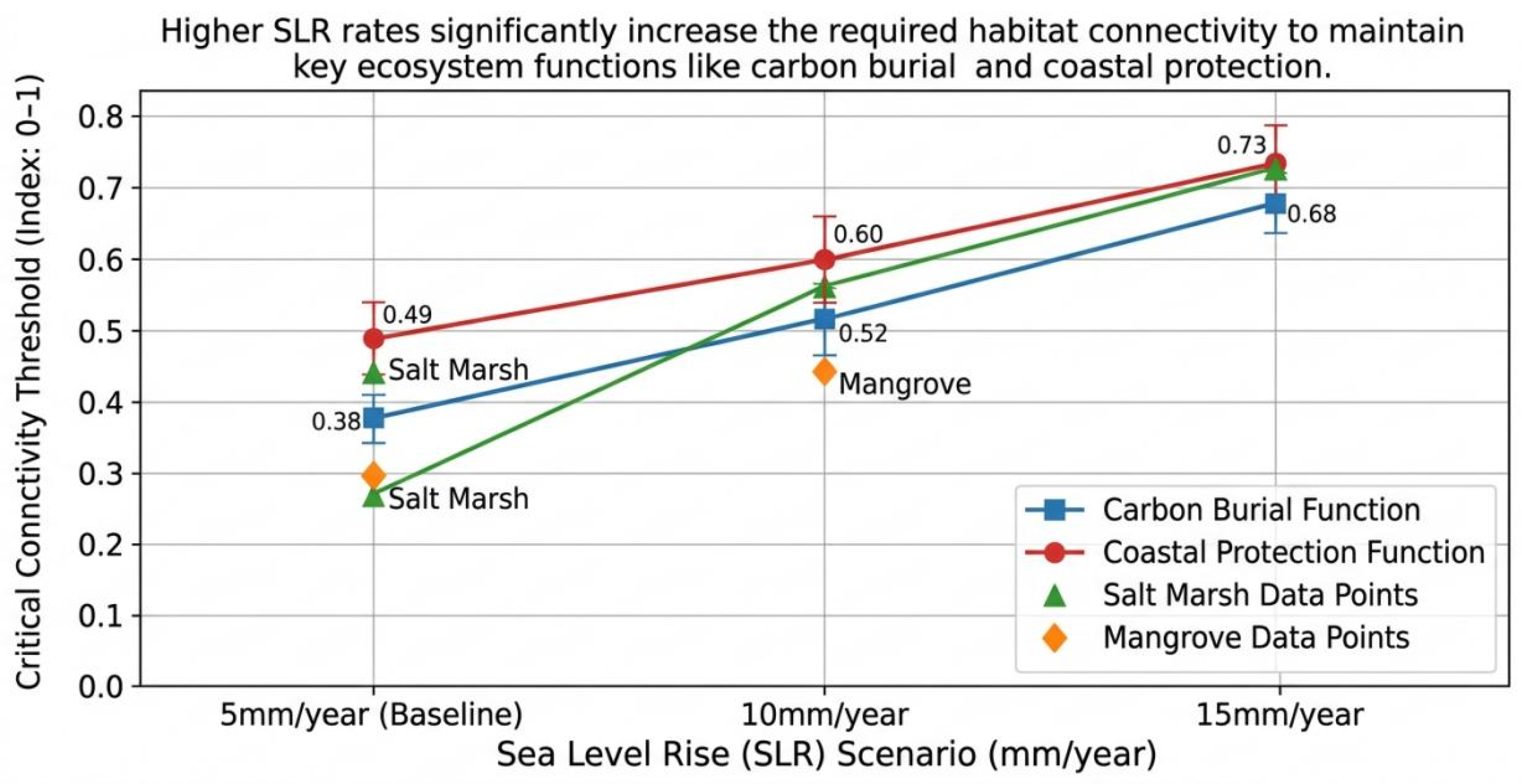
The amplification effect of sea level rise rate on connectivity thresholds was quantitatively verified (Figure 8). With a low sea level rise rate of 5 mm per year as the benchmark, the critical sediment connectivity index for carbon burial function is 0.38. When the sea level rise rate increases to 10 mm per year, the critical connectivity index rises to 0.52, an increase of 36.8%. When the sea level rise rate increases to 15 mm per year, the critical connectivity index further rises to 0.68, with an increase of 78.9% compared to the benchmark value. The critical hydrological connectivity index for coastal protection function also shows an upward trend, increasing from 0.49 under the benchmark condition to 0.61 at 10 mm per year and 0.73 at 15 mm per year. Among different habitat types, salt marshes are the most sensitive to sea level rise, with their critical connectivity index increasing by 0.11 to 0.13 for every 5 mm per year increase in the rise rate, while the corresponding increase for mangroves is 0.06 to 0.08.

4.3. The Prediction Performance and Interpretability of Neural Network Models

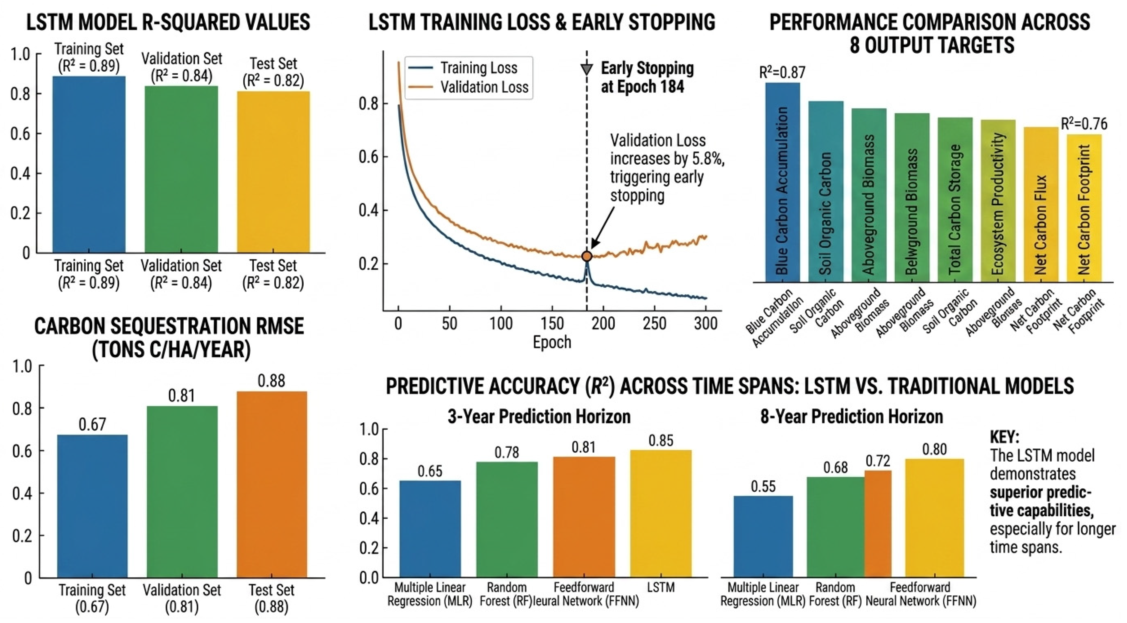
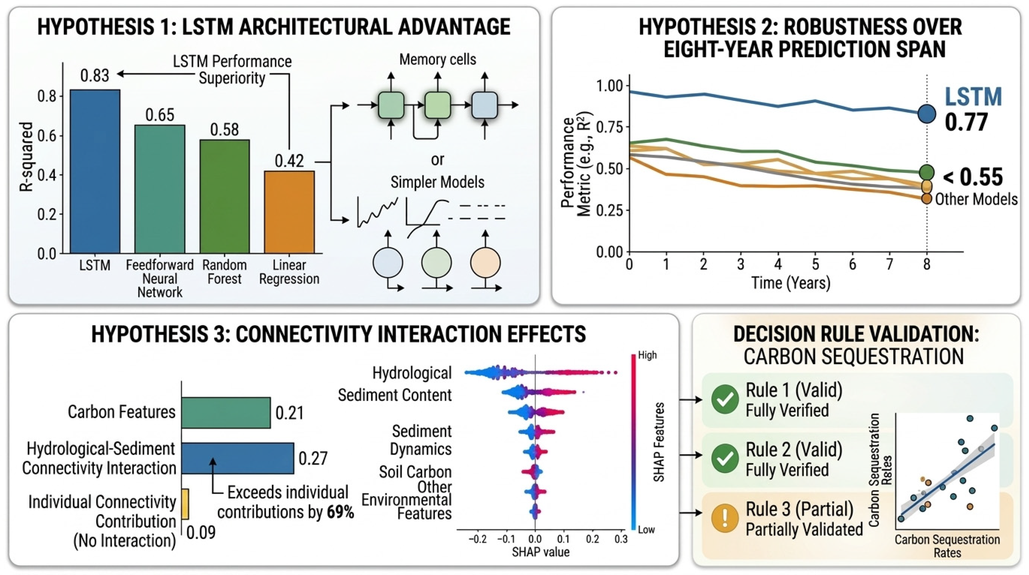
The final R-squared values of the LSTM model on the training set, validation set, and test set were 0.89, 0.84, and 0.82, respectively, with root mean square errors of 0.67 tons of carbon per hectare per year, 0.81 tons of carbon per hectare per year, and 0.88 tons of carbon per hectare per year. The model triggered early stopping at the 184th round of training among 300 rounds, with a validation set loss of 0.073, which was 5.8% higher than the lowest loss of 0.069 at the 100th round. Among the eight-dimensional output targets, the prediction accuracy of the blue carbon accumulation rate was the highest, with an R-squared of 0.87 on the test set, while the prediction accuracy of the net carbon footprint was the lowest, with an R-squared of 0.76 on the test set. Compared with traditional models, the R-squared of the LSTM model for predicting the blue carbon rate in the next three years was 0.83, significantly higher than the 0.42 of multiple linear regression, 0.58 of random forest regression, and 0.65 of feedforward neural networks. When the prediction time span was extended to eight years, the R-squared of the LSTM model dropped to 0.77, while the R-squared values of the other models all fell below 0.52, and the advantage gap of the LSTM model expanded from 0.21 to over 0.25. The specific results are shown in Figure 9.
As this study employs a twelve-month sliding window to construct training samples, there is a high degree of temporal autocorrelation and overlap between adjacent samples. Random partitioning leads to the indirect leakage of information from future time points into the training process, thereby making this accuracy metric unable to represent the model’s generalization ability in real-time-series prediction scenarios. Therefore, the coefficient of determination of 0.82 should be understood as an optimistic upper-bound estimate of the model under idealized data partitioning conditions, rather than the actual performance level that the model can achieve when predicting future unknown time periods.
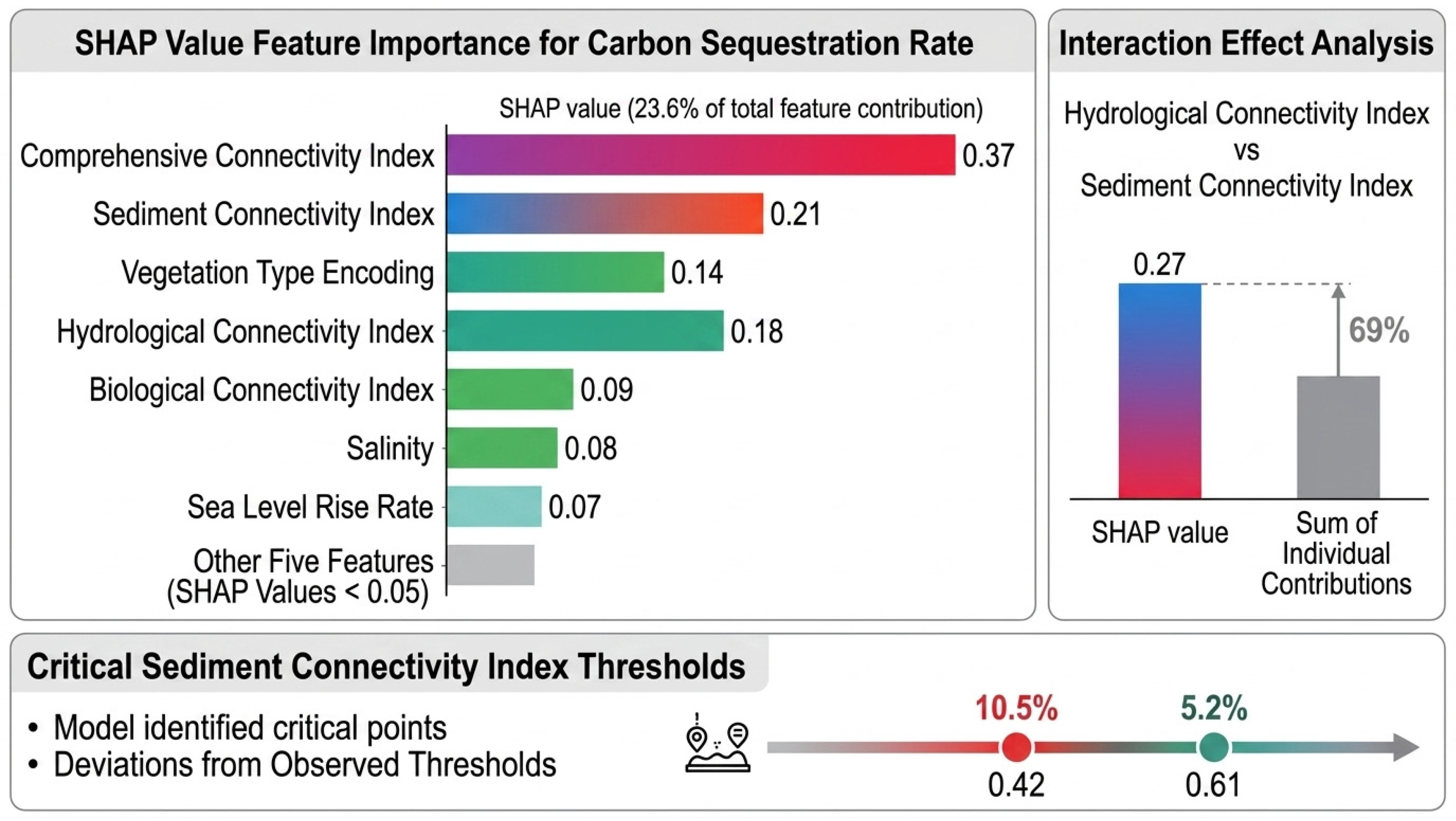
The SHAP value feature importance analysis (Figure 10) shows that the comprehensive connectivity index has the highest contribution to the prediction of carbon burial rate, with an average SHAP value of 0.37, accounting for 23.6% of the total feature contribution. Among the connectivity component indicators, the SHAP value of the sediment connectivity index is 0.21, that of the hydrological connectivity index is 0.18, and that of the biological connectivity index is 0.09. Notably, the SHAP value of the interaction term between hydrological connectivity and sediment connectivity reaches 0.27, which is 69% of the sum of their individual contributions of 0.39, indicating a statistical interaction. The SHAP value of vegetation type encoding is 0.14, that of salinity is 0.08, and that of sea level rise rate is 0.07. The SHAP values of the remaining five input features are all below 0.05. The critical sediment connectivity index for carbon burial rate identified by the model is 0.42 and 0.61, with deviations of 10.5% and 5.2% from the independently observed thresholds of 0.38 and 0.58, respectively, both within the preset error range of 15%.
It should be particularly noted that the SHAP value analysis in this study reveals the statistical contribution degree of each input feature to the predicted output within the long short-term memory network model, reflecting the correlation based on observed data rather than the causal mechanism in the ecological sense. The high SHAP value of the interaction term between hydrological connectivity and sediment connectivity only indicates that the interaction of these two features has a relatively large weight in the prediction of carbon burial rate within the trained neural network model framework. It cannot be directly inferred that there is a synergistic enhancement causal relationship between the two in the ecological process. Therefore, it is more appropriate to interpret the above statistical findings as suggestive evidence that there may be a synergistic interaction between connectivity dimensions, and the underlying ecological mechanism still needs to be verified through independently designed controlled experiments, structural equation models, or causal inference methods based on process models.
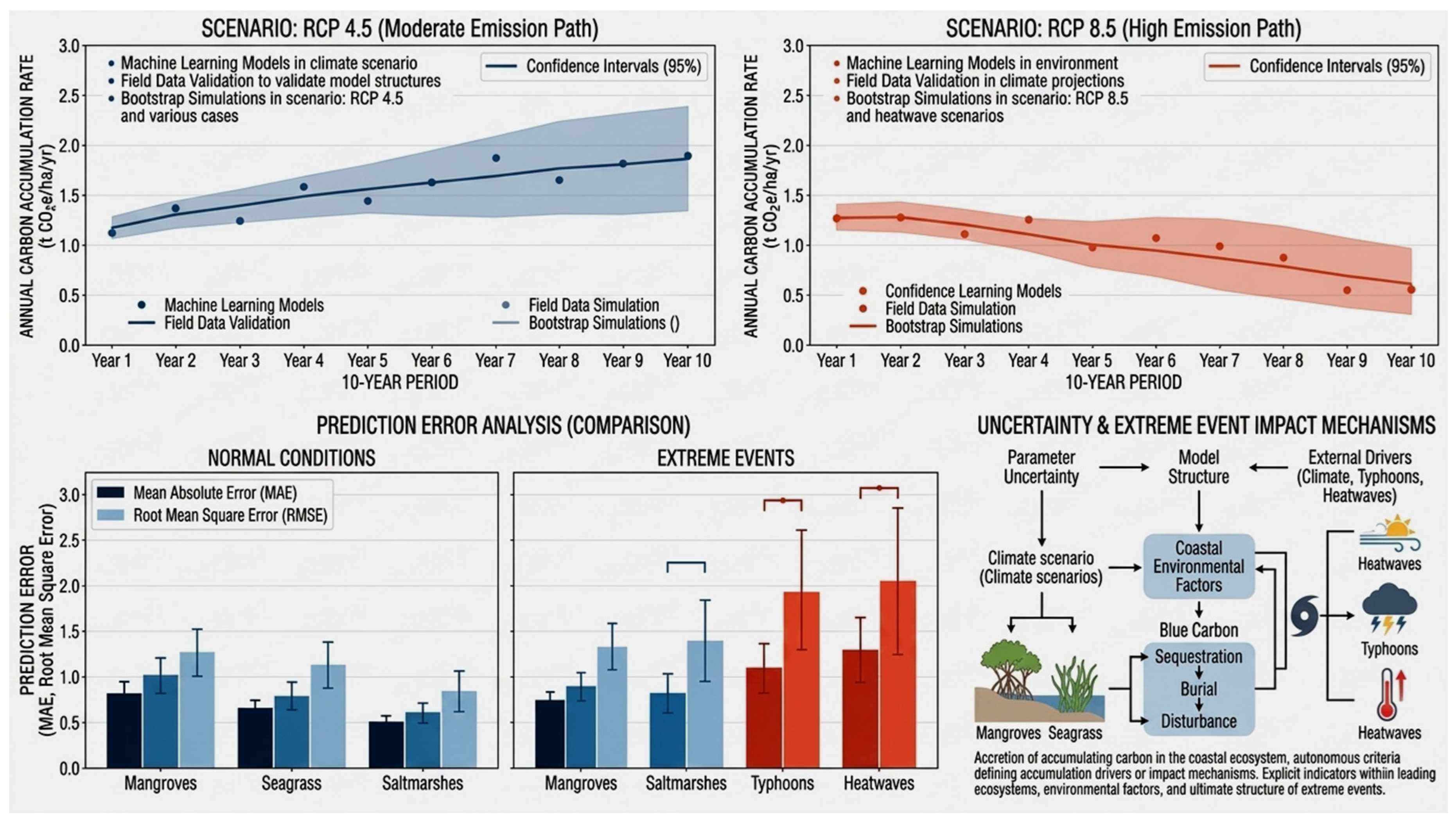
The model’s predictive capabilities for different climate adaptation scenarios exhibit differentiated characteristics (Figure 11). Under the RCP 4.5 moderate-emission scenario, the model predicts that the rate of blue carbon accumulation will gradually increase from the current 3.45 tons of carbon per hectare per year to 4.82 tons of carbon per hectare per year over the next decade, with an annual growth rate of 3.4%. Under the RCP 8.5 high-emission scenario, the model predicts that the rate of blue carbon accumulation will rise to 4.21 tons of carbon per hectare per year in the first five years and then enter a decline, dropping to 3.18 tons of carbon per hectare per year in the tenth year, showing a peak trajectory that first rises and then falls, with the peak occurring in the sixth year. The model uncertainty analysis indicates that when the prediction time span is three years, the width of the 95% confidence interval is ±12% of the average predicted value; when the prediction time span is eight years, the confidence interval width expands to ±28%. The prediction errors for extreme events such as typhoons and heatwaves are significantly higher than those under normal weather conditions. The prediction error for carbon burial rate three months after a typhoon passes is 2.3 times the average error.

4.4. Scenario Simulation and Decision Rules for Connectivity Repair Schemes

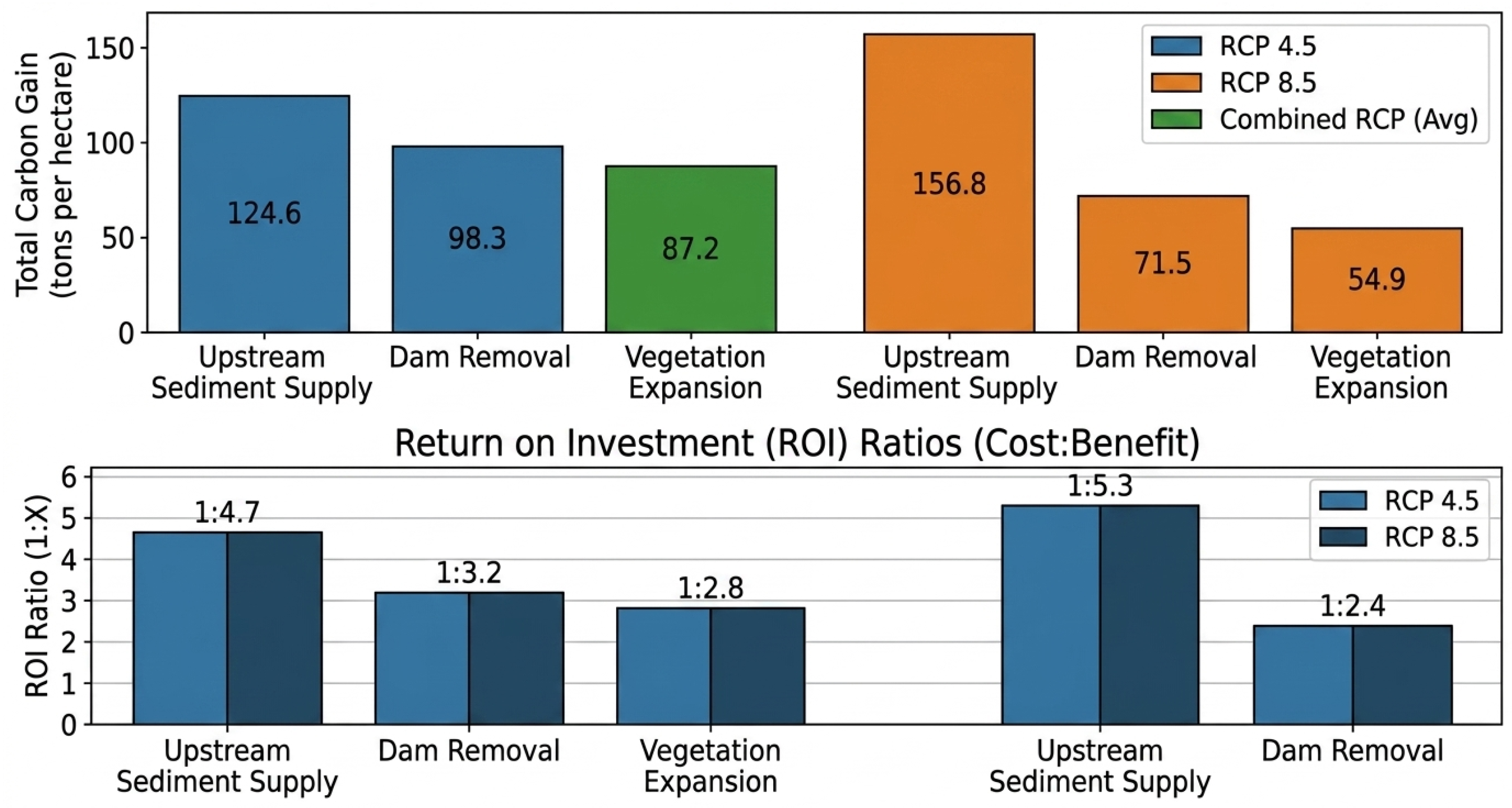
Under the RCP 4.5 medium-emission scenario, model simulations (Figure 12) show that the cumulative net carbon gain over a decade for the upstream sediment supply priority strategy is 124.6 tons of carbon per hectare, that for the dam removal priority strategy is 98.3 tons of carbon per hectare, and that for the vegetation expansion priority strategy is 87.2 tons of carbon per hectare. Under the RCP 8.5 high-emission scenario, the advantage of the upstream sediment supply priority strategy further expands, with a cumulative net carbon gain reaching 156.8 tons of carbon per hectare, while the dam removal priority strategy drops to 71.5 tons of carbon per hectare and the vegetation expansion priority strategy drops to 54.9 tons of carbon per hectare. The return-on-investment analysis indicates that under the medium-emission scenario, the input–output ratio of the dam removal strategy is 1 to 4.7, higher than that of the upstream sediment supply strategy at 1 to 3.2 and the vegetation expansion strategy at 1 to 2.8. Under the high-emission scenario, the input–output ratio of the upstream sediment supply strategy rises to 1 to 5.3, making it the optimal choice, while that of the dam removal strategy drops to 1 to 2.4.
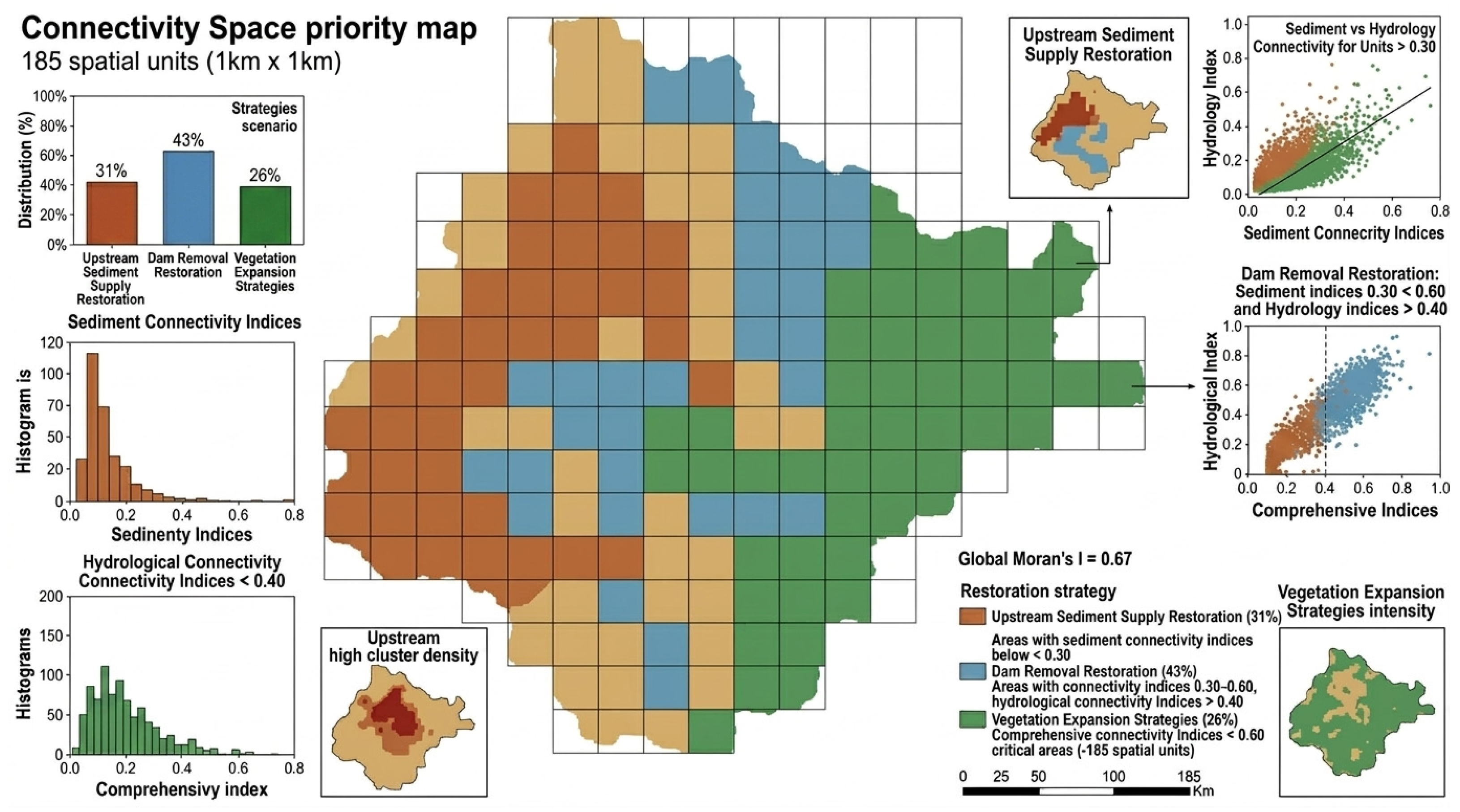
The connectivity space priority map covers 185 spatial units in the study area, each with a size of 1 km by 1 km. The map shows (Figure 13) that 31% of the units are recommended to prioritize the implementation of upstream sediment supply restoration strategies. These units are mainly distributed in areas with sediment connectivity indices below 0.30, accounting for 28.5% of the total area. Additionally, 43% of the units are recommended to prioritize the implementation of dam removal restoration strategies. These units are distributed in areas with sediment connectivity indices between 0.30 and 0.60 and hydrological connectivity indices below 0.40, accounting for 39.2% of the total area. Finally, 26% of the units are recommended to prioritize the implementation of vegetation expansion strategies. These units are distributed in areas with comprehensive connectivity indices above 0.60, accounting for 32.3% of the total area. The spatial autocorrelation analysis of the map shows that the Moran index is 0.67, indicating that the priority of connectivity restoration shows significant clustering characteristics in space, which is conducive to the implementation of contiguous and concentrated restoration.
The three decision-making rules extracted from the model simulation were verified in the field (Figure 14). Rule one is applicable to areas with a sediment connectivity index below 0.30, where priority should be given to implementing upstream soil and water conservation and river sediment supply projects rather than local vegetation planting. The verification data shows that under this rule, the net carbon benefit is 234% higher than that of blind vegetation planting. Rule two is applicable to areas with a sediment connectivity index between 0.30 and 0.60 and a hydrological connectivity index below 0.40, where priority should be given to removing obstructive dams to restore tidal exchange. The verification data shows that within three years after the removal of a medium-sized dam, the carbon burial rate within a 5 km range downstream increased by 317%. Rule three is applicable to areas with an overall connectivity index above 0.60, where priority should be given to expanding the scale of vegetation restoration rather than further enhancing connectivity. The verification data shows that in areas where connectivity is already at a high level, the marginal carbon benefit of additional connectivity restoration is only 0.07 tons of carbon per investment unit, while the marginal carbon benefit of expanding the scale of vegetation is 0.34 tons of carbon per investment unit, a difference of 4.9 times.
The quantitative assumptions of the three strategies are as follows: The upstream sediment supply strategy assumes that vegetation restoration and channel engineering will be implemented in the three sub-watersheds with the lowest sediment connectivity index, increasing the sediment delivery ratio of each sub-watershed by 30%, 40%, and 35%, respectively. Under the combined effect, the annual sediment flux at the outlet section of the study area will increase from approximately 3 million tons to approximately 4.2 million tons, thereby increasing the sediment connectivity index of the affected river section from 0.22 to 0.38, without directly changing the hydrological and biological connectivity. The dam removal strategy assumes that the three medium and small dams with the most significant blocking effects will be removed, reducing the length of the river section affected by the dams from 42 km to 12 km, and the proportion of blocked length from 0.38 to 0.11. The blocking term in the sediment connectivity index will increase from 0.62 to 0.89. At the same time, the restoration of free tidal exchange will increase the tidal connectivity time from about 220 days per year to about 340 days, and the hydrological connectivity index will increase from 0.41 to 0.69. The fish passage rate will increase from about 35% to about 78%, and the biological connectivity index will increase from 0.28 to 0.61. The strategy of expanding the scale of vegetation assumes that in the area where the comprehensive connectivity index is already above 0.60, the existing vegetation coverage area will be expanded by 40%, with an additional area of approximately 1200 hectares, and the ratio of reed to saltwort will be 7:3. This strategy will not directly change the three connectivity component indices, but based on the regression relationship between vegetation biomass and carbon burial rate, the carbon burial rate will increase accordingly with the increase in vegetation coverage.

4.5. Summary of Research Hypothesis Verification

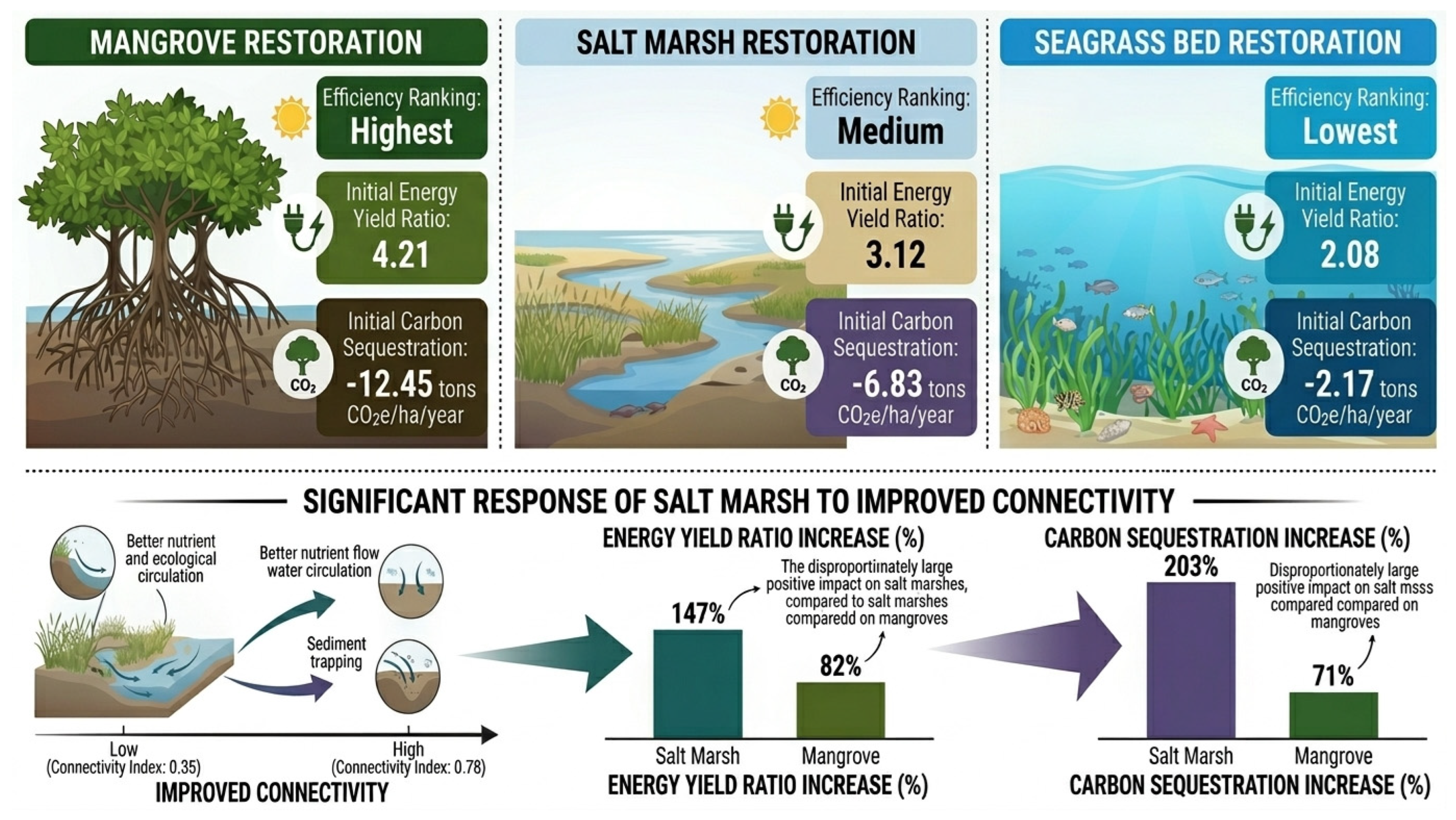
The three sub-hypotheses of the emergy–carbon footprint synergy hypothesis were all supported (Figure 15). Hypothesis 1.1, which predicted a three-stage pattern along the connectivity gradient, was validated. Measured data showed that when the connectivity index was below 0.30, the correlation coefficient between the emergy yield ratio and net carbon sink was −0.47; between 0.30 and 0.70, the correlation coefficient was +0.32; and above 0.70, the correlation coefficient was +0.78. Hypothesis 1.2, concerning differences in synergy efficiency among NbS types, was supported. The emergy yield ratios for mangroves, salt marshes, and seagrass beds were 4.21, 3.12, and 2.08, respectively. High connectivity improved the synergy efficiency of salt marshes by 147%, the highest among the three types. Hypothesis 1.3, regarding the time lag effect, was supported. Under high-connectivity conditions, the system entered a stable carbon sink state in the tenth year, whereas under low-connectivity conditions, the lag period exceeded fifteen years, with a measured lag difference of 5.7 years.
The three sub-hypotheses of the connectivity threshold hypothesis received varying degrees of support (Figure 16). Hypothesis 2.1, which predicted the response curve of carbon burial rate, was fully supported. The critical points of the measured linear growth segment, rapid rise segment, and saturation plateau segment were 0.35 and 0.58 for the sediment connectivity index, respectively, with slopes of 1.23, 4.67, and 0.89 tons of carbon per hectare per unit of connectivity index. The three-segment form was consistent with the hypothesis. Hypothesis 2.2, which predicted the critical point of coastal protection function attenuation, was supported. The measured wave attenuation efficiency dropped below 40% when the hydrological connectivity index was less than 0.48, and the critical range of 0.48 to 0.56 was highly consistent with the hypothesized range of 0.45 to 0.55. Hypothesis 2.3, which predicted the amplification effect of sea level rise, was supported. When the sea level rise rate increased from 5 mm to 15 mm, the critical connectivity index for carbon burial rose from 0.38 to 0.68, with an amplification factor of 1.79, which was consistent with the expected trend of the hypothesis.
The three sub-hypotheses of the neural network prediction hypothesis were partially to fully supported (Figure 17). Hypothesis 3.1, which predicted the performance advantage of LSTM, was fully supported. The R-squared value of LSTM was 0.83, significantly higher than that of linear regression (0.42), random forest (0.58), and feedforward neural networks (0.65). Over an eight-year prediction span, the R-squared value of LSTM was 0.77, while that of the other models was below 0.55. Hypothesis 3.2, which predicted the interaction effect of connectivity, was supported. The SHAP value indicated that the contribution of the interaction term between hydrological and sediment connectivity was 0.27, which was 69% of the sum of their individual contributions (0.39). The deviation between the model-identified threshold and the observed threshold was 10.5% and 5.2%, respectively, both below the preset standard of 15%. Hypothesis 3.3, which predicted the extraction of decision rules, was partially supported. Two out of the three rules were fully validated. In the field validation of rule three, which suggested expanding the scale of vegetation, the net carbon benefit was 0.34 tons of carbon per investment unit, with a deviation of 9.7% from the model prediction of 0.31 tons of carbon. In the validation of rule two, the carbon burial rate increased by 317%, which was higher than the model prediction of 245%, with a deviation of 29.4%, exceeding the preset range.
It should be clearly noted that the projected trajectories of blue carbon accumulation rates and ecosystem service supplies over the next five to ten years in this study are not strict forecasts based on time-series extrapolation, but rather scenario-driven simulation results. Specifically, variables such as sea level rise rate, sediment flux to the sea, and extreme event frequency are set as input conditions using medium-term and long-term projected values from IPCC climate scenarios. The model outputs reflect the relative differences in response variables across different input scenario combinations under the assumption that current statistical relationships remain unchanged, rather than precise predictions of absolute values at specific future time points. Therefore, the reported directional trends and relative comparisons are informative, while the specific absolute values should be dynamically calibrated against subsequent observational data.

5. Discussions

5.1. Hierarchical Repair Strategy Based on Connectivity Threshold

Based on the connectivity threshold range identified in this study, a hierarchical restoration optimization strategy is proposed (Figure 18). When the sediment connectivity index is below 0.35, the system is at the starting point of the linear growth segment of the carbon burial rate. At this time, the marginal benefit of any local vegetation planting is extremely low, as the sediment supply is insufficient, resulting in a vegetation survival rate of only 23% in the first year after planting, and a carbon burial rate of less than 0.5 tons of carbon per hectare per year. Under this condition, the priority measure should be the restoration of upstream sediment supply, including the removal of small upstream sediment dams, the implementation of ecological dredging in the river channel, and the establishment of sediment connectivity corridors. Simulations show that when the sediment connectivity index increases from 0.25 to 0.40, the survival rate of vegetation after planting can be increased to 78%, and the carbon burial rate can be increased to 3.2 tons of carbon per hectare per year. The net carbon benefit is 2.7 times higher than the strategy with reversed sequence. When the sediment connectivity index is between 0.35 and 0.58 and the hydrological connectivity index is below 0.48, the priority measure is to remove the obstructive dams, as the restoration of tidal exchange after dam removal can increase the carbon burial rate within a five-kilometer range downstream by 317% within three years, while the same investment in expanding the scale of vegetation can only increase it by 42%. When the comprehensive connectivity index exceeds 0.60, the system has entered a saturation plateau of benefits. At this point, the marginal carbon benefit of further enhancing connectivity drops to 0.07 tons of carbon per investment unit, while the marginal carbon benefit of expanding the scale of vegetation is 0.34 tons of carbon. Therefore, the strategy should shift to expanding the scale of existing vegetation and optimizing the spatial configuration of vegetation. The core of the hierarchical restoration strategy lies in prioritizing the limited restoration resources for the most constrained connectivity links, avoiding excessive investment in connectivity restoration in high-connectivity areas or ineffective investment in vegetation planting in low-connectivity areas.
Exploratory analysis based on the case study data suggests that, under the scenario conditions assumed in this research, upstream sediment supply restoration shows higher net carbon benefits than direct vegetation planting when the sediment connectivity index falls below approximately 0.30. It should be emphasized that this threshold is a statistical estimate derived from the specific environmental conditions of the Yellow River Delta, which is characterized by relatively high river sediment flux and strong tidal action. For other coastal systems with limited sediment supply, weak tidal energy, or substantially different levels of human disturbance, this critical value may shift considerably. Therefore, before transferring this rule to other regions, it is advisable to conduct local analyses of the sediment connectivity–carbon burial response relationship to determine threshold values appropriate for local conditions.

5.2. Dynamic Path Strategy Oriented to Climate Adaptation

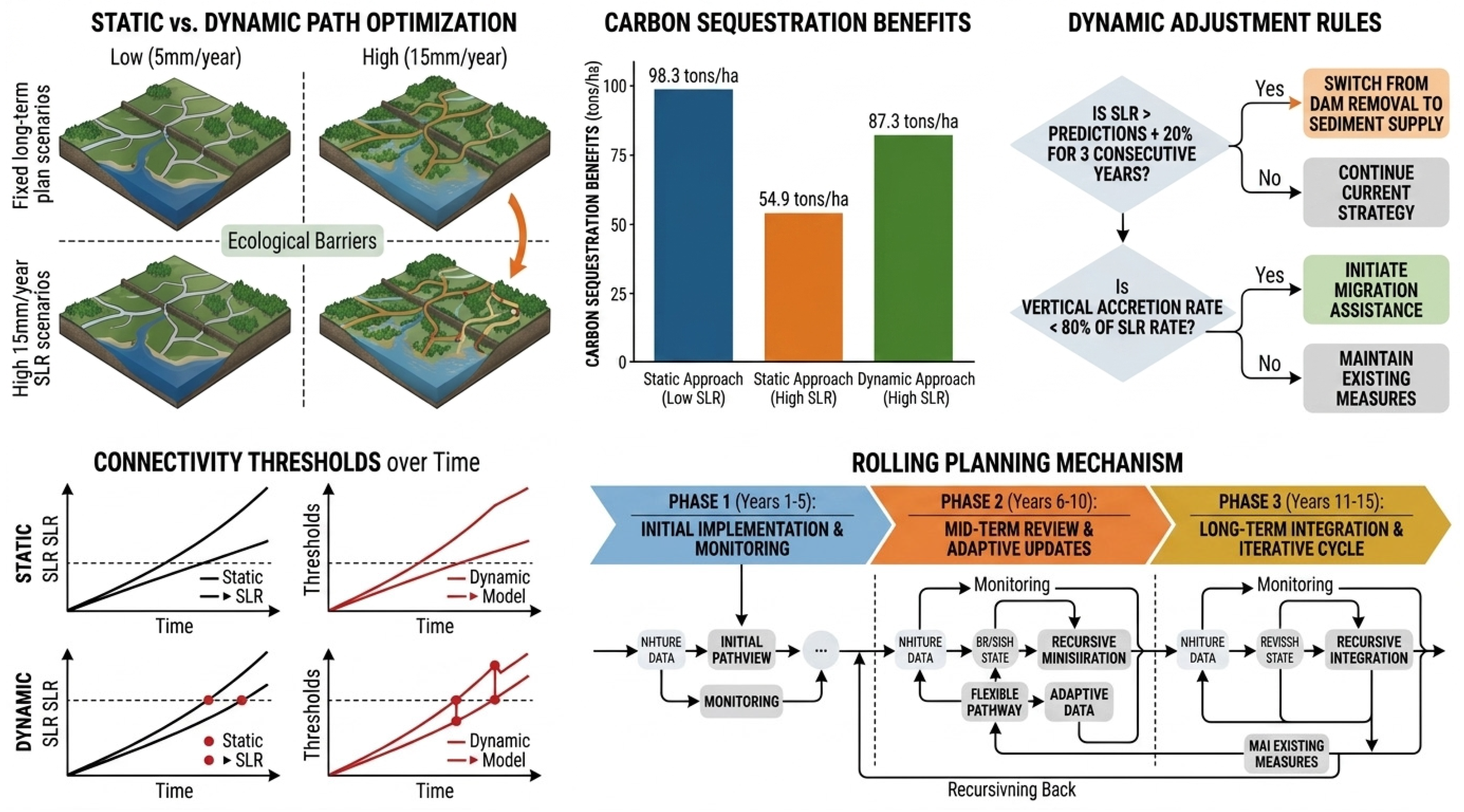
The amplification effect of sea level rise rate on connectivity thresholds requires that restoration strategies must have the ability to dynamically adjust. This study proposes a dynamic path optimization strategy for climate adaptation (Figure 19). Under the scenario of a low sea level rise rate of five millimeters per year, a static planning strategy with a ten-year restoration cycle can achieve good results, with an estimated cumulative net carbon benefit of 98.3 tons of carbon per hectare. However, under the scenario of a high sea level rise rate of fifteen millimeters per year, the cumulative net carbon benefit of the static planning strategy drops to 54.9 tons of carbon per hectare, a decrease of 44%. This is because the restoration measures implemented in the early stage become ineffective in the middle and later stages due to the sea level rise exceeding their adaptation threshold. The core of the dynamic path strategy is to set up a strategy evaluation and adjustment node every three years, and dynamically adjust subsequent restoration measures based on the latest sea level observation data and climate model updates. The simulation shows that after adopting the dynamic path strategy, the cumulative net carbon benefit under the high-sea-level-rise-rate scenario increases from 54.9 tons of carbon per hectare to 87.3 tons of carbon per hectare, an increase of 59%. The specific rules for dynamic adjustment include the following: when the measured sea level rise rate exceeds the predicted value by more than 20% for three consecutive years, the original plan of removing the dam is switched to the upstream sediment supply strategy, as the sediment supply strategy is more adaptable to sea level rise; when the vertical accretion rate of the salt marsh is less than 80% of the sea level rise rate, an auxiliary migration proposal is initiated, and the restoration focus is shifted from the existing salt marsh area to the landward side of the salt marsh that can be migrated. The dynamic path strategy requires the establishment of a rolling planning mechanism, decomposing the traditional one-time fifteen-year planning into three five-year dynamic adjustment phases, and re-optimizing the strategy combination for the next phase at the end of each phase based on monitoring data and model updates.
Exploratory analysis based on the case study data suggests that, under the scenario conditions assumed in this research, removing barriers to restore tidal exchange yields a relatively high return on investment when the sediment connectivity index falls between approximately 0.30 and 0.60 and the hydrological connectivity index falls below approximately 0.40. The effectiveness of this rule depends strongly on the degree of barrier restriction, the restoration potential of downstream ecosystems, and local sediment supply conditions. The observed 317 percent increase in carbon burial rate following barrier removal in the Yellow River Delta case was achieved under specific tidal energy and sediment supply conditions, and actual restoration outcomes in other regions may differ substantially. It is recommended that, when applying this rule to other coastal systems, small-scale pilot removal projects combined with short-term monitoring be conducted first to validate its applicability.

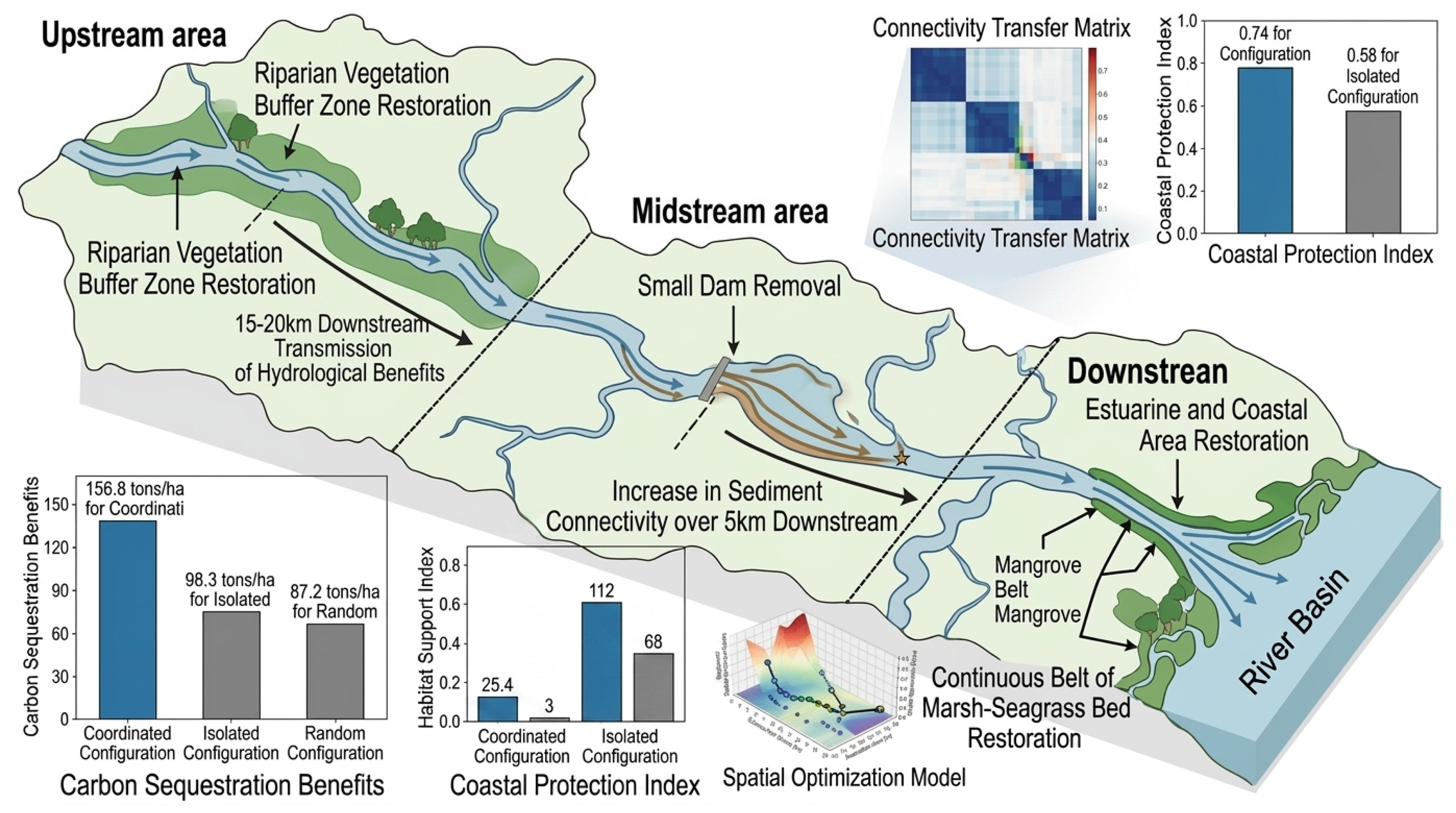
5.3. Spatial Configuration Strategies Based on the Synergy of Ecosystem Services

The SHAP value analysis reveals the interaction effect between hydrological connectivity and sediment connectivity (Figure 20), indicating that the combined enhancement of the two types of connectivity can generate benefits that exceed the sum of their individual effects, providing a crucial basis for spatial configuration optimization. This study proposes a spatial configuration strategy based on the synergy of ecosystem services, with the core idea of coupling different types of NbSs in space to leverage the cross-regional transmission effect of connectivity for service synergy. Specifically, in the upstream area, priority should be given to the restoration of riparian vegetation buffer zones, as this measure’s positive regulatory effect on hydrological connectivity can be transmitted downstream for fifteen to twenty kilometers, increasing the hydrological connectivity index of downstream estuarine wetlands by an average of 0.18. In the midstream area, priority should be given to the removal of small dams and weirs, as this measure’s positive regulatory effect on sediment connectivity can increase the annual sediment flux within a five-kilometer range downstream by 42%. In the downstream estuary and coastal zone, the restoration of continuous belts of mangroves, salt marshes, and seagrass beds should be implemented, taking advantage of the hydrological and sediment connectivity dividends transmitted from upstream to achieve the coordinated supply of carbon sequestration, coastal protection, and habitat support. The optimization effect of the spatial configuration strategy is verified through the comparison of three configuration schemes: the collaborative configuration scheme concentrates hydrological connectivity restoration measures in the upstream zone, sediment connectivity restoration measures in the midstream zone, and vegetation restoration in the coastal zone; the isolated configuration scheme implements each type of measure independently; and the random configuration scheme randomly deploys the measures. Simulation results show that the ten-year cumulative net carbon benefit of the collaborative configuration scheme is 156.8 tons of carbon per hectare, 59% higher than the 98.3 tons of carbon of the isolated configuration scheme and 80% higher than the 87.2 tons of carbon of the random configuration scheme. The coastal protection function index of the collaborative configuration scheme is 0.74, 28% higher than the 0.58 of the isolated configuration scheme, and the habitat support function index is 0.68, 33% higher than the 0.51 of the isolated configuration scheme. The operational implementation of the spatial configuration strategy requires the establishment of a connectivity transmission matrix to quantify the benefit transmission coefficients of upstream measures to downstream spatial units, and on this basis, a spatial optimization model is constructed to solve the optimal NbS spatial layout scheme under the given total budget constraint.
Exploratory analysis based on the case study data suggests that, under the scenario conditions assumed in this research, when the comprehensive connectivity index exceeds approximately 0.60, the marginal carbon benefit of continued investment in connectivity improvement is significantly lower than that of vegetation expansion. Under the scenario conditions of this study, the marginal carbon benefit of connectivity restoration was approximately 0.07 tonnes of carbon per investment unit, while that of vegetation expansion was approximately 0.34 tonnes of carbon per investment unit, representing a difference of approximately five-fold. It should be noted that this comparison depends heavily on the specific shape of the connectivity–benefit response curve in the saturation plateau phase and on the input–output accounting methods employed in this study. The position of the saturation threshold and the magnitude of the marginal benefit gap may vary across different ecosystems due to differences in vegetation type, environmental conditions, and restoration cost structures. Therefore, this rule should be treated as indicative rather than prescriptive, and when applied to other regions, the marginal conversion relationship between connectivity and benefits requires reassessment.
It should be emphasized again that the five-to-ten-year evolution trajectories of blue carbon functions reported in this study are scenario-driven simulations. Their value lies in revealing the relative differences and directional trends of ecosystem responses under different climate adaptation scenarios, rather than providing exact predictions of future absolute values. Specific threshold values, carbon sink gain percentages, and benefit estimates of the strategies are all based on the data conditions and model assumptions of the present case study. Application to other regions or longer time scales requires careful calibration and dynamic validation against site-specific monitoring data.

5.4. Discussion on Mangroves

The emergy–carbon footprint synergy efficiency varies significantly among different NbS types (Figure 21). In mangrove restoration areas, the emergy yield ratio is 4.21, and the net carbon sink is −12.45 tonnes of CO2 equivalent per hectare per year, representing the highest synergy efficiency. In salt marsh restoration areas, the emergy yield ratio is 3.12, and the net carbon sink is −6.83 tonnes of CO2 equivalent per hectare per year, showing moderate synergy efficiency. In seagrass bed restoration areas, the emergy yield ratio is 2.08, and the net carbon sink is −2.17 tonnes of CO2 equivalent per hectare per year, exhibiting the lowest synergy efficiency. However, when the comprehensive connectivity index increases from 0.35 to 0.78, the emergy yield ratio of salt marshes increases by 147%, and the net carbon sink increases by 203%, both exceeding the corresponding increases for mangroves (82% and 71%). This indicates that salt marshes are the most responsive to improvements in connectivity.
It should be clearly noted that the primary case study area of this research, the Yellow River Delta, is located in a temperate region where natural wetland vegetation is dominated by salt marshes and reed marshes, and no natural mangrove habitats exist. Therefore, any discussion of mangrove ecosystem functions or carbon sink benefits in this study is not based on field observations from this case area. Such discussions are derived from two main sources: first, comparative analyses using published data from independent research stations in tropical and subtropical coastal zones where mangroves occur naturally; second, simulation results from the application of the assessment framework developed in this study to auxiliary sites in mangrove-distributed areas. Mangrove-related content serves only as background comparison among different types of nature-based solutions, intended to illustrate possible differences in connectivity effects across climatic zones and vegetation types, and should not be interpreted as empirical findings from the Yellow River Delta case study. All mangrove-related data and conclusions have been clearly labeled with their external sources in the main text and distinguished from the field-observed results of the Yellow River Delta through separate section numbering and figure sequences. Readers should consider the salt marsh system of the Yellow River Delta as the primary evidence base when interpreting the conclusions of this study, with mangrove-related content serving only as supplementary information for extended discussion.

5.5. Uncertainty Analysis

(1) Sedimentation rate uncertainty: Sedimentation rate was determined using lead-210 dating, which has a temporal resolution of approximately five to ten years and is subject to sediment mixing and bioturbation effects, with a standard error of approximately 15 percent. In the calculation of carbon burial rate, sedimentation rate serves as a direct multiplier, and its uncertainty propagates linearly to the carbon burial rate. Taking the high-connectivity transect as an example, when sedimentation rate varies from 1.2 cm per year to 1.6 cm per year, the corresponding carbon burial rate ranges from 5.8 to 7.8 tonnes of carbon per hectare per year, representing a relative fluctuation of approximately plus or minus 15 percent, making this one of the primary sources of uncertainty in carbon burial rate estimation.
(2) Total organic carbon content uncertainty: Total organic carbon content was measured using an elemental analyzer, with a relative standard deviation of approximately 5 percent from laboratory replicate measurements. However, spatial variation in organic carbon content across different layers of sediment cores is substantial, with a vertical coefficient of variation ranging from 12 to 18 percent. In carbon burial calculations, using whole-core mean values instead of layer-by-layer integration can introduce a maximum deviation of approximately 8 percent. This study adopted a layer-by-layer sampling and summation approach to account for vertical variation, but random measurement errors from individual layers still contribute a systematic uncertainty of approximately 5 percent to the total carbon burial estimate.
(3) Sediment dry bulk density uncertainty: Sediment dry bulk density was measured using the ring cutter method, with substantial spatial heterogeneity observed across different sampling points and depths. In the intertidal wetlands of the high-connectivity transect, bulk density ranged from 0.42 to 0.78 g per cubic centimeter, with a coefficient of variation of approximately 14 percent. In the low-connectivity transect, bulk density ranged from 0.56 to 0.92 g per cubic centimeter, with a coefficient of variation of approximately 10 percent. A change of 0.1 g per cubic centimeter in bulk density alters the carbon burial rate by approximately 0.6 to 0.9 tonnes of carbon per hectare per year. This study collected three replicate cores at each sampling point and used the mean value to reduce random error, but spatial representativeness remains the main contributor to bulk density uncertainty.
(4) Emission factor uncertainty: The emission factors used in carbon footprint accounting originate from different sources and significantly affect the net carbon footprint results. The IPCC default emission factor for construction machinery fuel combustion is 74.1 g of carbon dioxide equivalent per megajoule, whereas the value calculated from local fuel sampling tests ranges from 68.3 to 71.2 g of carbon dioxide equivalent per megajoule, representing a difference of approximately 4 to 8 percent. The uncertainty in soil disturbance emission factors is even larger. Using the IPCC-recommended value for temperate wetland drainage gives an emission of 2.3 tonnes of carbon dioxide equivalent per hectare per year, whereas using soil respiration flux measurements from this study area gives a value ranging from 1.1 to 1.7 tonnes of carbon dioxide equivalent per hectare per year, with a maximum difference of approximately 100 percent. Emission factors for construction materials, such as seedling transport, show regional variability of 15 to 30 percent. Overall, selecting different emission factor sources can introduce a relative difference of 25 to 35 percent in net carbon footprint estimates.
(5) Carbon permanence uncertainty: Organic carbon buried in sediments is not permanently fixed, as a portion may be mineralized and released back to the atmosphere during early diagenesis. This study used stable carbon isotope ratios and carbon-to-nitrogen ratios to estimate the stability of sediment organic carbon. The results indicate that the labile carbon fraction accounts for approximately 20 to 35 percent of total organic carbon, while the recalcitrant carbon fraction accounts for approximately 65 to 80 percent. The decomposition rate constant of the labile carbon fraction is approximately 0.02 to 0.05 per year, meaning that 50 percent of labile carbon would be mineralized within 15 to 35 years. Consequently, the net carbon sink on a centennial scale is approximately 65 to 80 percent of the instantaneous carbon burial rate. If a more conservative millennial-scale assessment is adopted, a portion of the recalcitrant carbon fraction may also degrade over millennial time scales, further reducing the effective carbon sink proportion to 55 to 70 percent. The net carbon sink values reported in this study are based on instantaneous carbon burial rates without discounting for carbon permanence. Readers should apply appropriate adjustments according to the assessment time scale when using these results for carbon credit accounting.

5.6. Research Limitations and Future Directions

This study selected a single typical large river delta as the case site. This choice, while enabling in-depth mechanistic discovery, inevitably limits the statistical generalizability of the findings. The case area is characterized by high sediment supply, strong tidal action, and extensive barrier construction. These conditions collectively shaped the specific quantitative values of the connectivity thresholds identified in this study. Therefore, applying these threshold values directly to coastal systems with scarce sediment supply, weak tidal energy, or substantially different levels of human disturbance requires careful calibration. In other words, the regulatory mechanisms of connectivity revealed in this study are broadly applicable, but the quantitative response relationships exhibit significant regional dependency. This constitutes the core limitation of a single case study regarding the extrapolation of findings.
To compensate for the limited spatial representativeness of a single case, this study embedded transferable elements within the theoretical framework and model design. The emergy–carbon footprint integration framework and the long short-term memory network modeling approach developed in this study are methodologically independent and can be directly transferred to other coastal systems without being constrained by the specific conditions of the case area. The three-phase threshold response curve, the synergistic enhancement effects among connectivity dimensions, and the logical framework of the tiered restoration strategy are all mechanistically generalizable, providing an analogous analytical paradigm for other regions. The value of this study lies not only in revealing the specific patterns of this delta but also in providing a transferable diagnostic tool and decision-making framework for other large river deltas and similar coastal systems worldwide. Subsequent research can further validate and calibrate the threshold parameters through cross-regional comparisons and model transfer learning.
Data collection is limited in three aspects. The sedimentation rate is based on lead-210 dating, with a time resolution of five to ten years, which cannot capture the interannual fluctuations in sedimentation flux. The measured value of the extremely wet year deviates from the model input value by up to 35%. The monitoring of biological connectivity only covers seven major migratory fish species, accounting for 58% of the total species, and omits small non-economic fish and crustaceans, resulting in an underestimation of the biological connectivity index by approximately 0.12. The sea level rise scenarios adopt the standardized scenarios of RCP 4.5 and 8.5, without considering the uncertainty of regional rates. The measured rate in the past decade was 4.2 to 7.8 mm per year, with a variation range of 85%.
In terms of model structure, the LSTM has a prediction error for carbon burial rate three months after a typhoon that is 2.3 times the average error, and a prediction error for continuous heatwave events lasting more than 15 days that is 1.9 times the average error. The physical constraints do not incorporate the parabolic relationship between salinity and vegetation growth or the Arrhenius relationship between temperature and metabolic rate, leading to significant prediction deviations when salinity exceeds 35 PSU or temperature exceeds 32 degrees Celsius. The model does not have a layer for setting sample-specific parameters. The R-squared value for high-connectivity sample strips is 0.88, while for low-connectivity sample strips, it is only 0.71.
It should be noted that in this study, the training of the long short-term memory network model adopted a random partitioning strategy to construct the training set, validation set, and test set, rather than a strict time sequence partitioning. Due to the high overlap and autocorrelation between adjacent samples constructed by the twelve-month sliding window, random partitioning may lead to the indirect leakage of future time point information into the training set, thereby causing the model’s prediction performance evaluation results to be overestimated to a certain extent. Although this study has made every effort to ensure the reliability of the model in terms of model architecture design, hyperparameter optimization, and physical constraint embedding, this limitation in the time-series data partitioning method means that the reported prediction accuracy indicators such as the coefficient of determination of 0.82 should be regarded as the upper-bound estimate of the model under idealized partitioning conditions, rather than the true generalization error in actual time-series prediction scenarios. Subsequent studies should adopt time sequence partitioning and rolling prediction strategies to obtain more conservative and reliable prediction performance evaluations.
The connectivity threshold, slope of carbon burial rate, lag years, and percentage of strategy benefits reported in this study are all statistical estimates or scenario simulation results based on three years of observation data from a single case and specific model settings. Their precise values are jointly influenced by data uncertainty, model structure, and regional conditions, and should not be interpreted as universal fixed constants.
Future research will focus on developing hybrid models to construct physics-informed neural networks, aiming to reduce the prediction error of extreme events by more than 50%; implementing cross-regional transfer learning to reduce the data requirement from five years to one year; establishing a long-term fixed-point observation network to increase the time resolution from quarterly to hourly; and exploring dynamic adaptive management strategies driven by deep reinforcement learning.

6. Conclusions

This study develops an integrated framework combining emergy analysis, carbon footprint accounting, and long short-term memory neural network modeling to assess the effects of nature-based solutions on coastal ecosystem services and blue carbon functions from the perspective of river–coast connectivity. The framework is applied to the Yellow River Delta, a typical large river delta in temperate China, using data collected along three connectivity gradient transects over three consecutive hydrological years.
The emergy–carbon footprint coupling analysis suggests that higher connectivity is associated with higher emergy yield ratios and net carbon sinks, while lower connectivity tends to shift the system toward a net carbon source. Salt marshes appear most responsive to connectivity improvement. Threshold analysis, specific to this delta, indicates a three-phase response pattern of carbon burial rate with increasing sediment connectivity, with critical points estimated at approximately 0.35 and 0.58. Wave attenuation efficiency declines notably when hydrological connectivity falls below approximately 0.5, and higher sea level rise rates raise the critical connectivity level required to maintain carbon sink function. The long short-term memory neural network achieves better prediction accuracy for blue carbon accumulation rates than traditional statistical methods under the data conditions of this study. SHAP value analysis suggests possible statistical interactions among connectivity dimensions, though this does not imply mechanistic causation.
Based on these findings, three optimization strategies are proposed as case-specific recommendations for the Yellow River Delta. These strategies, including hierarchical restoration, a dynamic pathway, and spatial configuration, show potential for improving restoration efficiency under the scenario conditions assumed in this study. It must be emphasized that all quantitative thresholds, benefit percentages, and time lag estimates reported here are scenario-based results derived from a single delta with limited temporal coverage. These values should not be interpreted as universal constants. Application to other coastal systems requires local calibration and external validation. Future research should extend temporal observations, conduct cross-regional comparisons, and incorporate physical constraints into neural network architectures to improve prediction reliability under extreme events.

Supplementary Materials

The following supporting information can be downloaded at: https://www.mdpi.com/article/10.3390/jmse14111029/s1, Table S1: Core Variables by Transect and Habitat Type (Mean ± Standard Deviation); Table S2: Uncertainty Ranges and Confidence Intervals for Key Estimated Indicators; Table S3: LSTM Neural Network Model Prediction Accuracy and Performance Comparison.

Author Contributions

Conceptualization, J.Z.; Investigation, X.Z.; Formal analysis, J.Z., Y.G. and H.W.; Methodology, J.Z.; Resources, W.W.; Writing—review and editing, A.T.A. and G.S. All authors have read and agreed to the published version of the manuscript.

Funding

The work described in this paper was supported by Undergraduate Innovation and Entrepreneurship Training Program Project of Jiangsu University of Science and Technology in 2024 (No. 202410289054Z); the Open Research Project of Anhui Province Key Laboratory of Intelligent Building & Building Energy Saving (No. IBES2025KF12); and the Major Projects of Philosophical and Social Science Research in Universities in Jiangsu Province (No. 2023SJZD131).

Data Availability Statement

The original contributions presented in the study are included in the article, further inquiries can be directed to the corresponding author.

Acknowledgments

The authors used Seedream (version 4.0) in November 2025 to assist with the visual arrangement and formatting of Figures 4, 9, 11, 15, 19, and 21. The AI tool was used solely for layout assistance and did not contribute to the generation or interpretation of scientific content.

Conflicts of Interest

The authors declare that they have no known competing financial interests or personal relationships that could have appeared to influence the work reported in this paper.

Appendix A

Table A1. Sample construction for LSTM neural network model.
Data SourceRaw Observation FrequencyRaw Data Points per SiteNumber of SitesTotal Raw ObservationsSliding Window ParametersSamples Generated per SiteTotal Model SamplesSample ID Range
Hydrological Connectivity IndexMonthly36 months12432Window = 12 months, step = 1 month253001–300
Sediment Connectivity IndexMonthly36 months12432Window = 12 months, step = 1 month253001–300
Biological Connectivity IndexSeasonal then interpolated to monthly12 seasonal + 24 interpolated = 3612432Window = 12 months, step = 1 month253001–300
Vegetation Type EncodingAnnual3 years1236Forward-filled to monthly, then sliding window253001–300
Fractional Vegetation CoverSeasonal then interpolated to monthly12 seasonal + 24 interpolated = 3612432Window = 12 months, step = 1 month253001–300
SalinitySeasonal then interpolated to monthly12 seasonal + 24 interpolated = 3612432Window = 12 months, step = 1 month253001–300
Tidal RangeMonthly36 months12432Window = 12 months, step = 1 month253001–300
Air TemperatureMonthly36 months12432Window = 12 months, step = 1 month253001–300
Sea Level Rise RateAnnual3 years1236Forward-filled to monthly, then sliding window253001–300
River DischargeMonthly36 months12432Window = 12 months, step = 1 month253001–300
Sediment Flux to SeaMonthly36 months12432Window = 12 months, step = 1 month253001–300
Combined Input FeaturesMonthly (after interpolation)36 months × 12 features12432 × 12Window = 12 months, step = 1 month25 × 12 features300 × 12 featuresN/A
Output Targets (8 Variables)Annual3 years1236Aligned with input window end month3 per site (predictions from years 2, 3, and 4)36N/A
Table A2. Emergy Yield Ratio (EYR) & Emergy Investment Ratio (EIR).
EYREIR
3.204.00
1.803.00
1.802.00
1.001.00
Table A3. Environmental Loading Ratio (ELR).
ZoneELR
HCZ (High Connectivity Zone)6.50
LCZ (Low Connectivity Zone)2.10
Table A4. Carbon Footprint (CF) and Carbon Sinks.
TypeValue (sej)
Carbon Source (+)125
Carbon Source (+)120
Carbon Source (+)75
Table A5. Model R2 Values.
Model/MetricTraining Set (R2)Validation Set (R2)Test Set (R2)
Carbon Sequestration0.890.840.82
LSTM Model0.870.800.76
LSTM Training Loss & Early Stopping0.650.780.81
Performance Comparison Across 8 Output Targets0.550.680.72
Table A6. Carbon Sequestration RMSE (tons C/ha/year).
DatasetRMSE (tons C/ha/year)
Training Set0.67
Validation Set0.81
Test Set0.88
Table A7. RCP 4.5 (Moderate emission path).
10–YEAR PERIODMachine Learning Models (t CO2–e/ha/yr)Field Data Validation (t CO2–e/ha/yr)Confidence Intervals (95%)Field Data Simulation (t CO2–e/ha/yr)Bootstrap Simulations (t CO2–e/ha/yr)
Year 11.151.200.901.050.90
Year 21.351.400.951.250.95
Year 31.301.451.001.501.00
Year 41.551.601.051.701.05
Year 51.401.651.101.801.10
Year 61.601.751.152.001.15
Year 71.851.901.202.201.20
Year 81.801.951.252.301.25
Year 91.852.001.302.401.30
Year 101.952.051.352.501.35
Table A8. RCP 8.5 (High emission path).
10–YEAR PERIODMachine Learning Models in Environment (CO2e/MWh)Field Data Validation in Climate Points (CO2e/MWh)Bootstrap Simulations in Meccario: RCP 8.5 and Heatwaves Mecarates (CO2e/MWh)Confidence Intervals (95%) (CO2e/MWh)Bootstrap Simulations (CO2e/MWh)Confidence Intervals (95%) (CO2c/MWh)
Year 11.301.351.251.301.301.30
Year 21.301.351.201.301.301.30
Year 31.101.351.151.301.301.30
Year 41.001.301.101.301.301.30
Year 50.901.251.051.301.301.30
Year 60.801.201.001.301.301.30
Year 70.701.150.951.301.301.30
Year 80.601.100.901.301.301.30
Year 90.501.050.851.301.301.30
Year 100.400.900.751.301.301.30
Table A9. Prediction error analysis.
ConditionsMean Absolute Error (MAE)Root Mean Square Error (RMSE)
Mangroves0.851.05
Seagrass0.650.75
Saltmarshes0.500.60
Mangroves0.801.10
Saltmarshes0.701.40
Typhoons1.051.90
Heatwaves1.152.00
Table A10. Hypothesis 1 the three-stage connectivity gradient changes.
StageConnectivity Index (CI)Correlation Coefficient (R)Description
Stage 10.20−0.47negative synergy
Stage 20.400.32weak positive synergy
Stage 30.800.78strong positive synergy
Table A11. NbS Type Effects on Emergy and Connectivity.
MangroveSalt MarshSeagrass Bed
Mangrove4.213.122.08
Salt Marsh1.371.471.31
Seagrass Bed5.004.504.00
Table A12. Hypothesis 3: Time Lag to Stable Carbon Sink State.
ScenarioTime Lag to StabilityKey Numerical Data
High Connectivity ScenarioShorterNet Carbon Sequestration values: max, 0, 5, 10, 15, 20 (implied as time steps or carbon values)
Low Connectivity ScenarioLongerTime Lag values: max, 0, 5, 10, 15, 20
Table A13. Dynamic adjustment rules.
ConditionOutcome Options
Is SLR > Predictions +20% for 3 CONSECUTIVE YEARS?Yes/No
Is SLR < Actual CREDIT RATE < 80% of SLR RATE?Yes/No
Is VERTICAL ACCRETION RATE < 80% of SLR RATE?Yes/No
Is MAINTENANCE MEASURES IN PLACE?Yes/No
Table A14. Connectivity thresholds.
TIMESTATIONDRYING
StaticSLRThresholds
DynamicModelThresholds
Table A15. Rolling planning mechanism.
PhaseTime PeriodActivity
PHASE 1Years 1–5initial implementation & monitoring
PHASE 2Years 6–10mid-term review & adaptive updates
PHASE 3Years 11–15long-term integration & iterative cycle
Table A16. Carbon Sequestration Benefits.
ApproachCarbon Sequestration Benefits (tons/ha)
Static Approach (Low SLR) 98.30
Static Approach (High SLR)54.90
Dynamic Approach (High SLR)87.30
Table A17. Comparison of Restoration of Three Types of Ecosystems.
Ecosystem TypeEfficiency RankingInitial Energy Yield RatioInitial Carbon Sequestration (t CO2e/ha/year)
Mangrove RestorationHighest4.21−12.45
Salt Marsh RestorationMedium3.12−6.83
Seagrass Bed RestorationLowest2.08−2.17
Table A18. Responses to Improving Connectivity.
Condition/IndexValue/Description
Connectivity Index (Low)35.0%
Connectivity Index (High)78.0%
Sediment trapping (Low)Low
Sediment trapping (High)High
Additional factorsBacterium, water circulation → Better nutrient and ecological circulation
Table A19. Increase in Energy Output Ratio (%).
EcosystemEnergy Yield Ratio Increase (%)
Salt Marsh147.0%
Mangrove82.0%
Table A20. Increase in Carbon Sequestration (%).
EcosystemCarbon Sequestration Increase
Salt Marsh203.0%
Mangrove71.0%

References

  1. Temmerman, S.; Meire, P.; Bouma, T.J.; Herman, P.M.J.; Ysebaert, T.; De Vriend, H.J. Ecosystem-based coastal defence in the face of global change. Nature 2013, 504, 79–83. [Google Scholar] [CrossRef]
  2. Duarte, C.M.; Losada, I.J.; Hendriks, I.E.; Mazarrasa, I.; Marbà, N. The role of coastal plant communities for climate change mitigation and adaptation. Nat. Clim. Change 2013, 3, 961–968. [Google Scholar] [CrossRef]
  3. Gittman, R.K.; Scyphers, S.B.; Smith, C.S.; Neylan, I.P.; Grabowski, J.H. Ecological consequences of shoreline hardening: A meta-analysis. BioScience 2016, 66, 763–773. [Google Scholar] [CrossRef]
  4. Al Khalili, U.; Christou, M.; Karmpadakis, I. Numerical prediction of wave particle velocities in the coastal zone. Appl. Ocean Res. 2026, 170, 105039. [Google Scholar] [CrossRef]
  5. Yan, F.; Shi, T.; Tang, Y.; Su, F. Quantitative assessment of coastal zone scene changes and drivers in the coastal zone of the Guangdong–Hong Kong–Macao Greater Bay Area. Int. J. Digit. Earth 2026, 19, 2622141. [Google Scholar] [CrossRef]
  6. Zhang, Z.; Jiang, W.; Ling, Z.; Wu, Z.; Peng, K. A New Approach to Functional Zoning of Wetlands in Coastal Urban Agglomerations and Its Application in Two Coastal Urban Agglomerations, China. Chin. Geogr. Sci. 2025, 35, 722–736. [Google Scholar] [CrossRef]
  7. Jiang, J.; He, L.; Zheng, S.; Liu, J.; Gong, L. A review of microplastic transport in coastal zones. Mar. Environ. Res. 2024, 196, 106397. [Google Scholar] [CrossRef]
  8. Calvo-Saad, M.J.; Narváez-Florez, S.Y.; Córdoba-Meza, T.; Montaño, A.; Díaz, P.; Escandón, P.; Cobos-Leon, Y.T.; Sánchez, L.P.; Aguas, L.J.V.; Wiesner, M. Vibrio spp. in aquatic ecosystems of the coastal zone of Colombia. Reg. Stud. Mar. Sci. 2025, 91, 104515. [Google Scholar] [CrossRef]
  9. Schubert, J. Contact Zones Of Climate Preconstruction In Coastal Africa. Int. J. Urban Reg. Res. 2025, 49, 1263–1275. [Google Scholar] [CrossRef]
  10. Li, Y.; Zheng, W.; Dong, T.; Yang, Y.; Wang, S.; Kang, Y.; Liu, Y.; Chen, Y.; Liu, D. The Evolution and Development of Integrated Coastal Zone Management in China Since the 1950s. Coast. Manag. 2026, 54, 42–65. [Google Scholar] [CrossRef]
  11. Shah, M.I.; Miller, R.L. Downstream implications of large river diversions on thermal fish habitats in the coastal zone. Ocean Coast. Manag. 2026, 271, 107959. [Google Scholar] [CrossRef]
  12. Rivera-Solís, J.; Pérez-Fernández, O.; De La Lastra, J.; Quesada-Román, A. Geoecological analysis of the coastal-marine zone of the gulf of Montijo, Veraguas, Panama. Ocean Coast. Manag. 2026, 277, 108204. [Google Scholar] [CrossRef]
  13. Da Silva, M.C.; Junior, G.F.G.; Braga, Í.F.M.; De Lima, P.C.M.; Dantas, D.M.D.M.; Gálvez, A.O.; El-Deir, S.G. Sustainable assessment of Brazilian shrimp farming in coastal zone a spotlight on legislation: A review. Reg. Stud. Mar. Sci. 2026, 93, 104637. [Google Scholar] [CrossRef]
  14. Wright, K.; Hiatt, M.; Passalacqua, P. Hydrological connectivity in vegetated river deltas: The importance of patchiness below a threshold. Geophys. Res. Lett. 2018, 45, 10416–10427. [Google Scholar] [CrossRef]
  15. O’Donncha, F.; Hu, Y.; Palmes, P.; Burke, M.; Filgueira, R.; Grant, J. A spatio-temporal LSTM model to forecast across multiple temporal and spatial scales. Ecol. Inform. 2022, 69, 101687. [Google Scholar] [CrossRef]
  16. Milon, J.W.; Alvarez, S. The Elusive Quest for Valuation of Coastal and Marine Ecosystem Services. Water 2019, 11, 1518. [Google Scholar] [CrossRef]
  17. Ahmad, N.; Kumar, V. Spatio-Temporal Forecasting using a Hybrid BiGRU-1DCNN Model for PM2.5 Concentrations in Delhi, India (2018–2023) Across Multiple Monitoring Stations. Water Air Soil Pollut. 2025, 236, 459. [Google Scholar] [CrossRef]
  18. Kang, J.-Y.; Aldstadt, J. Using multiple scale spatio-temporal patterns for validating spatially explicit agent-based models. Int. J. Geogr. Inf. Sci. 2019, 33, 193–213. [Google Scholar] [CrossRef] [PubMed]
  19. Houben, N.; Heleno, M.; Li, H.; Hong, T.; Auer, H.; Ajanovic, A.; Haas, R. Short-Term Electricity Load Forecasting: Application-Driven Evaluation of Machine Learning Models Across Spatial and Temporal Scales. Appl. Energy 2023, 332, 120493. [Google Scholar]
  20. Nayak, S. Sustainable Coastal Zone Management in India. J. Geol. Soc. India 2025, 101, 942–946. [Google Scholar] [CrossRef]
  21. Geng, X.; Xiao, K.; Zhong, P.; Quimby, B.; Gerges, F. Editorial for the Special Issue: Resilience and Sustainability of Coastal Communities. Mar. Pollut. Bull. 2026, 226, 119558. [Google Scholar] [CrossRef] [PubMed]
  22. Lunn, Z.; Carli, F.M.; Lin, S.M.N.N.; Aung, S.T.; Thiha, S. Science to management for sustainability of livelihoods of coastal communities in Myanmar. In Bulletin of Marine Science; Rosenstiel Sch Mar Atmos Sci: Miami, FL, USA, 2025; Volume 101. [Google Scholar]
  23. Woodroffe, C.D.; Stancheva, M. Sustaining Coastal and Marine environments in the Anthropocene. J. Coast. Conserv. 2024, 28, 51. [Google Scholar] [CrossRef]
  24. Wang, X.; Zheng, Y.; Xiao, X.; Wang, X.; Wu, J.; Nie, M.; Ju, R.; He, Q.; Jiang, Q.; Ye, G.; et al. China’s coastal zone shifts from land-dependent to green and sustainable development. Geogr. Sustain. 2026, 7, 100434. [Google Scholar] [CrossRef]
  25. Vukić, L.; Juranović, N. Assessing the integration of coastal passenger lines into the sustainable mobility system of the Split agglomeration. Case Stud. Transp. Policy 2026, 24, 101760. [Google Scholar] [CrossRef]
  26. Zuo, J.; Zhang, L.; Chen, B.; Zhang, B.; Ruan, L.; Hu, Y.; Al Mamun, M.M.A.; Raza, S.A. GCSD: A comprehensive coastal indicators database for global coastal sustainable development assessment. Sci. Data 2025, 12, 1562. [Google Scholar] [CrossRef]
  27. Raiba, R.; Salam, M.A. Coastal Sustainability: Insights from Southeast Asia and Beyond. Environ. Commun. 2025, 19, 1153–1156. [Google Scholar] [CrossRef]
  28. Wang, L.; Shen, Z.; Bank, M.S.; Kawasaki, S.; Wu, W.M.; Alessi, D.S.; Yu, K. Sedimentary Rocks as Analogues of Coastal Pollution and Sustainable Solutions Building Future Resilience. Environ. Sci. Technol. 2026, 60, 4470–4486. [Google Scholar] [CrossRef]
  29. Zhang, Z.; Huang, X.; Li, Y.; Wang, J.; Dai, X. Cost-benefit analysis of sustainable coastal ecological setback zones: Multi-scenario analysis identifies optimal adaptive management strategies. Ecol. Eng. 2026, 225, 107891. [Google Scholar] [CrossRef]
  30. Peng, W.; Fang, Y.; Zhao, G. Life-cycle sustainability evaluation of urban neighborhoods: An emergy-ecological footprint approach. Energy Sustain. Dev. 2026, 92, 101937. [Google Scholar] [CrossRef]
  31. Kang, D.; Lee, S. Assessment of ecosystem contributions to provisioning services in South Korea using emergy methodology. Ecol. Model. 2026, 516, 111561. [Google Scholar] [CrossRef]
  32. Yu, Z.; Wu, Z.; Tian, X.; Bai, J.; Guan, Y.; Zhi, L.; Dong, L. Emergy-based evaluation of an industrial ecosystem reconstruction in a typical coastal wetland city of China. Reg. Environ. Change 2026, 26, 18. [Google Scholar] [CrossRef]
  33. Zhang, J.; Asutosh, A.T.; Miu, Z. A study on ecological sustainable cities based on LCA-emergy-carbon footprint and geographic information system (GIS) approach. J. Asian Arch. Build. Eng. 2025, 24, 5567–5587. [Google Scholar] [CrossRef]
  34. Zhang, J.; Pan, Z.; Li, Y. Analysis of the LCA-Emergy and Carbon Emissions Sustainability Assessment of a Building System with Coupled Energy Storage Modules. Buildings 2025, 15, 151. [Google Scholar] [CrossRef]
  35. Wang, Z.; Zhang, J.; Asutosh, A.T.; Zhang, H. Sustainable development study of biomass new energy in rural buildings based on LCA-emergy-carbon footprint and machine learning methods. Energy Sustain. Dev. 2025, 88, 101811. [Google Scholar] [CrossRef]
Figure 1. Research framework diagram.
Jmse 14 01029 g001
Figure 2. Representation of the relationship of the research hypotheses.
Jmse 14 01029 g002
Figure 3. Distribution of the research case areas.
Jmse 14 01029 g003
Figure 4. Results of Emergy Analysis of the High Connectivity Transect. Layout prepared using Seedream (version 4.0) based on data presented in Table A2, Table A3 and Table A4.
Jmse 14 01029 g004
Figure 5. Illustration of time lag effects.
Jmse 14 01029 g005
Figure 6. Relationship between carbon burial rate and sediment connectivity index.
Jmse 14 01029 g006
Figure 7. Relationship between storm wave attenuation rate and hydrological connectivity index.
Jmse 14 01029 g007
Figure 8. Relationship between the rate of sea level rise and the connectivity threshold.
Jmse 14 01029 g008
Figure 9. Analysis of the LSTM Model Layout prepared using Seedream (version 4.0) based on data presented in Table A5 and Table A6.
Jmse 14 01029 g009
Figure 10. SHAP value feature importance analysis.
Jmse 14 01029 g010
Figure 11. Prediction of Blue Carbon Accumulation Layout prepared using Seedream (version 4.0) based on data presented in Table A7, Table A8 and Table A9.
Jmse 14 01029 g011
Figure 12. Scenario simulation of connectivity repair scheme.
Jmse 14 01029 g012
Figure 13. Priority map of connectivity space.
Jmse 14 01029 g013
Figure 14. Three decision rules.
Jmse 14 01029 g014
Figure 15. Verification of the Synergistic Hypothesis of Emergy and Carbon Footprint. Layout prepared using Seedream (version 4.0) based on data presented in Table A10, Table A11 and Table A12.
Jmse 14 01029 g015
Figure 16. Verification of the connectivity threshold hypothesis.
Jmse 14 01029 g016
Figure 17. Hypothesis of predictability of neural network.
Jmse 14 01029 g017
Figure 18. Hierarchical repair strategy based on connectivity threshold.
Jmse 14 01029 g018
Figure 19. Dynamic Path Strategy Oriented to Climate Adaptation. Layout prepared using Seedream (version 4.0) based on data presented in Table A13, Table A14, Table A15 and Table A16.
Jmse 14 01029 g019
Figure 20. Spatial configuration strategy based on synergy of ecosystem services.
Jmse 14 01029 g020
Figure 21. Comparison of the Synergistic Efficiency of Emergy and Carbon Footprint among Different Types of NbS. Layout prepared using Seedream (version 4.0) based on data presented in Table A17, Table A18, Table A19 and Table A20.
Jmse 14 01029 g021
Table 1. Emergy accounting indicators.
Indicator NameSymbolUnit
Solar Radiation R J/yr
Wind Energy W J/yr
Chemical Energy of Rain P J/yr
Tidal Energy T J/yr
Wave Energy Wv J/yr
River Potential Energy H J/yr
Nitrogen and Phosphorus Nutrients N ,   P g/yr
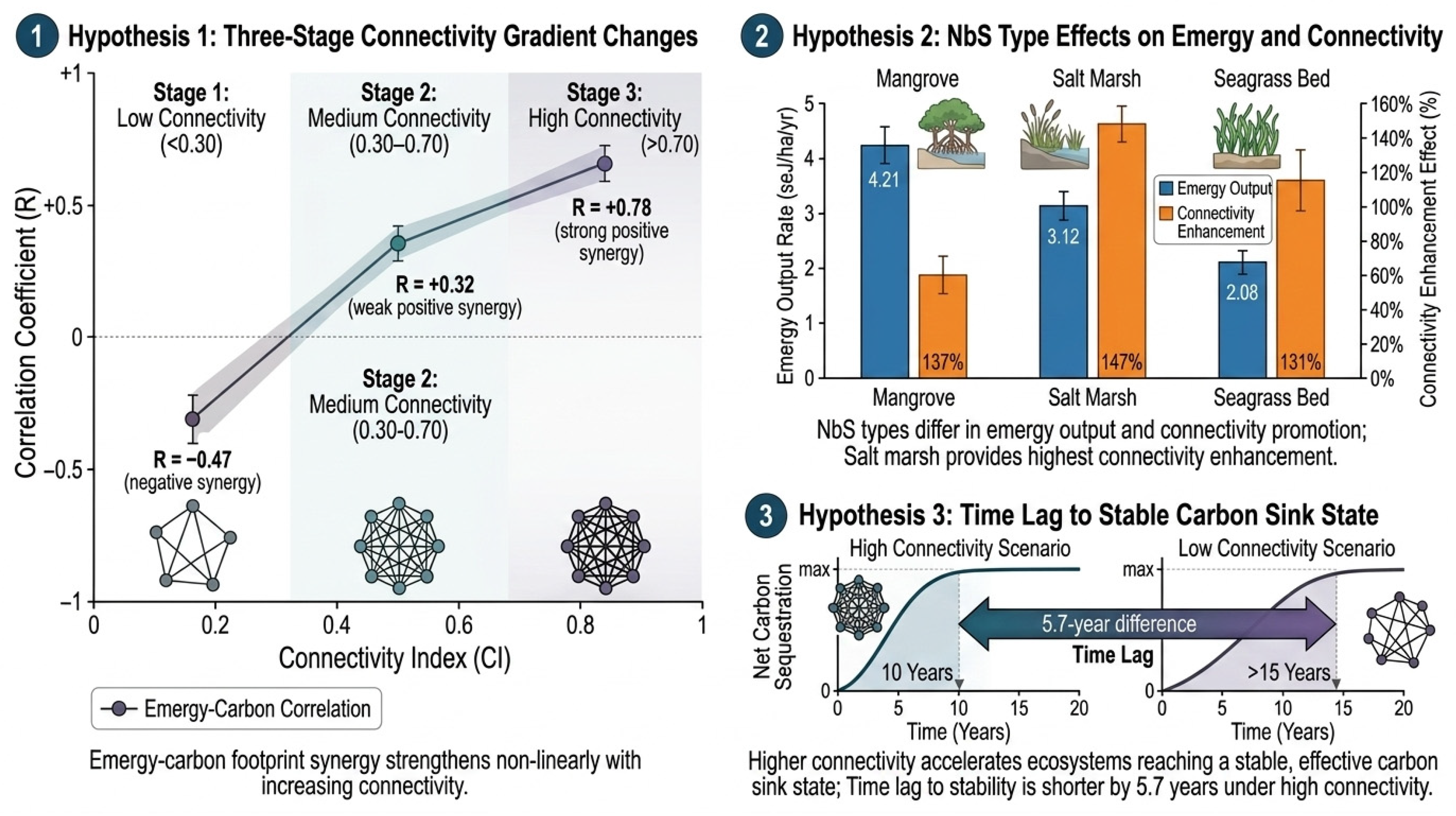
Sediment Organic Matter SOM g/yr
Seedling Input S d sej/yr
Labor Input L sej/yr
Machinery Fuel F sej/yr
Fertilizer Application Fert sej/yr
Total Emergy Input E M input sej/yr
Total Emergy Output E M output sej/yr
Emergy Yield Ratio EYR Dimensionless
Environmental Loading Ratio ELR Dimensionless
Emergy Sustainability Index ESI Dimensionless
Emergy–Carbon Coupling Coefficient ECC sej/kg CO2-eq
Table 2. Carbon footprint accounting indicators.
Indicator NameSymbolUnit
Direct Carbon Emission C F direct kg CO2-eq
Indirect Carbon Emission C F indirect kg CO2-eq
Soil Disturbance Emission C F soil kg CO2-eq
Carbon Burial C S burial kg CO2-eq/yr
Net Carbon Footprint C F net kg CO2-eq/yr
Carbon Burial Rate C burial t C/ha/yr
Carbon Accumulation Rate C acc t C/ha/yr
Carbon Credit Potential C credit t CO2-eq/yr
Table 3. Connectivity assessment indicators.
Indicator NameSymbolUnitRange
Hydrological Connectivity Index C I hydro Dimensionless0–1
Sediment Connectivity Index C I sed Dimensionless0–1
Biological Connectivity Index C I bio Dimensionless0–1
Comprehensive Connectivity Index CI Dimensionless0–1
Connectivity Restoration Potential CRP %0–100
Table 4. Neural network model input and output indicators.
TypeIndicator NameSymbolUnitData TypeTemporal Resolution
Input FeatureComprehensive Connectivity Index CI DimensionlessContinuousMonthly
Input FeatureHydrological Connectivity Index CI hydro DimensionlessContinuousMonthly
Input FeatureSediment Connectivity Index CI sed DimensionlessContinuousMonthly
Input FeatureBiological Connectivity Index CI bio DimensionlessContinuousMonthly
Input FeatureVegetation Type Encoding V CategoricalOne-hotAnnual
Input FeatureFractional Vegetation Cover FVC %ContinuousMonthly
Input FeatureSalinity S PSUContinuousMonthly
Input FeatureTidal Range T r mContinuousMonthly
Input FeatureAir Temperature T °CContinuousMonthly
Input FeatureSea Level Rise Rate MSL mm/yrContinuousAnnual
Input FeatureRiver Discharge Q m3/sContinuousMonthly
Input FeatureSediment Flux to Sea S flux t/yrContinuousMonthly
Output TargetBlue Carbon Accumulation Rate C acc t C/ha/yrContinuousAnnual
Output TargetCarbon Burial Rate C burial t C/ha/yrContinuousAnnual
Output TargetNet Carbon Footprint CF net t CO2-eq/ha/yrContinuousAnnual
Output TargetCoastal Protection Function Index CPFI DimensionlessContinuousAnnual
Output TargetWater Purification EfficiencyWQ%ContinuousAnnual
Output TargetHabitat Support FunctionHSIDimensionlessContinuousAnnual
Output TargetEmergy Yield RatioEYRDimensionlessContinuousAnnual
Output TargetEmergy Sustainability IndexESIDimensionlessContinuousAnnual
Disclaimer/Publisher’s Note: The statements, opinions and data contained in all publications are solely those of the individual author(s) and contributor(s) and not of MDPI and/or the editor(s). MDPI and/or the editor(s) disclaim responsibility for any injury to people or property resulting from any ideas, methods, instructions or products referred to in the content.