Article

Three-Dimensional Numerical Simulation of Near-Field Hydrodynamic Response and Suspended Sediment Transport Characteristics Around the Caofeidian Port Breakwaters

1
First Institute of Oceanography, Ministry of Natural Resources, Qingdao 266061, China
2
CCCC Water Transportation Consultants Co., Ltd., Beijing 100007, China
*
Author to whom correspondence should be addressed.
J. Mar. Sci. Eng. 2026, 14(11), 1018; https://doi.org/10.3390/jmse14111018
Submission received: 30 March 2026 / Revised: 17 April 2026 / Accepted: 22 April 2026 / Published: 29 May 2026
(This article belongs to the Section Ocean Engineering)

Abstract

Breakwater construction at meso-tidal ports fundamentally alters near-field hydrodynamics and drives harbor sedimentation, yet the three-dimensional mechanisms linking entrance geometry to sediment flux remain poorly quantified. Here, we apply a validated Delft3D tidal–sediment coupled model to Caofeidian Port, Bohai Bay, comparing pre-construction baseline conditions against four entrance width scenarios (400, 300, 250, and 200 m). Breakwater enclosure reduces depth-averaged harbor velocities by 61.9–63.2% during spring tides, while generating tip-jet velocities of 1.41–1.53 m s−1 at the eastern breakwater head—exceeding pre-construction maxima by 14–18%. The eastern tip produces an ebb vortex (radius ~230 m; peak vorticity 0.034 s−1) approximately 34% larger and 62% more intense than its flood counterpart, driving vortex-assisted sediment recirculation toward the harbor interior despite ebb-dominant background velocities. Reynolds flux decomposition confirms that the eastern tip-vortex sector contributes ~39% of net sediment import (advective component: −0.7%), directly quantifying vortex-assisted recirculation as an independent transport mechanism. Bed shear stress falls below the critical erosion threshold ( τ c e = 0.22 Pa) across 76.8% of the harbor area during spring tides (robust lower bound ~60% under wave-coupling correction), creating a structurally stable depositional interior, while the near-entrance zone sustains persistent tidal-cycle resuspension. Asymmetric tidal pumping—flood-phase open-sea SSC of 0.088 kg m−3 versus ebb-phase harbor SSC of 0.032–0.041 kg m−3—drives net spring-tide sediment import of 14.8 × 10⁶ kg per cycle (wave-coupled upper bound: 17.8–19.2 × 10⁶ kg per cycle). Entrance width reduction from 400 to 300 m achieves a favorable sedimentation-to-water exchange trade-off (marginal efficiency ratio 1.23), whereas further reduction to 200 m indicates onset of hydraulic choking. The marginal efficiency ratio declines sharply from 1.23 (400 → 300 m) to 1.03 (300 → 250 m) to 1.01 (250 → 200 m), indicating a hydraulic transition within the 250–300 m range that warrants targeted refinement in future studies.

1. Introduction

Bohai Bay has undergone one of the most intensive coastal reclamation programs in China over the past three decades. Since 2000, the cumulative reclaimed area has exceeded 1500 km2, fundamentally altering the tidal prism geometry, residual circulation patterns, and long-term sediment budget of the bay. Three-dimensional numerical studies of this transformation consistently document reductions in tidal prism of several percent alongside weakened water exchange capacity and modified suspended sediment flux pathways—consequences that scale with the spatial extent of reclamation rather than responding linearly to individual projects [1,2,3,4]. As a semi-enclosed basin operating near tidal resonance, the Bohai Sea is particularly sensitive to coastline modifications, with even modest changes in basin geometry producing nonlinear amplification or damping of tidal energy [5,6].
Caofeidian, projecting approximately 18 km into Bohai Bay from the Hebei coast, sits at the convergence of these bay-scale dynamics and port-scale engineering. Assessment using Lagrangian flow networks and information entropy theory shows that reclamation at Caofeidian increased input entropy near the port by approximately 160%, indicating that the modified coastline actively concentrates suspended material rather than merely rerouting it [7]. Bathymetric surveys spanning 2004–2021 document concurrent deepening of the natural channel adjacent to the headland—maximum water depth reached 42.3 m by 2021, with localized erosion rates up to −65 cm/a in the trough axis—reflecting the intensification of tidal energy concentration around the modified headland [8]. Morphodynamic modeling with Delft3D across five sequential reclamation phases showed that channel–shoal interactions responded non-uniformly to each construction stage, with net channel deepening in the main trough and shoaling on adjacent flats [9]—a pattern consistent with the geomorphic regime documented during early harbor construction [10].
The construction of enclosing breakwaters creates a near-field hydrodynamic environment qualitatively different from the open headland that previous bay-scale studies have characterized. Flow separation at breakwater tips generates persistent vortex structures whose properties depend on tidal phase, approach velocity, and structural geometry. Physical experiments and numerical simulations of seabed scouring around breakwaters at comparable meso-tidal port installations demonstrate that ebb-phase headland jets accelerate through the entrance aperture to velocities locally exceeding the pre-construction background, while the harbor interior simultaneously transitions to low-energy depositional conditions [11]. Wave–current interaction at the structure toe and the permeability of the breakwater itself further modulate the near-field regime [12,13], but these effects are secondary to the tidal-driven flow separation and vortex dynamics that are the focus of the present study.
Harbor sedimentation at meso-tidal ports involves several interacting mechanisms that observational data alone cannot readily disentangle. Port siltation studies at downdrift sites adjacent to river-influenced navigation channels document sediment input driven primarily by the phase relationship between tidal velocity and near-bed suspended sediment concentration rather than by mean residual transport [14,15]. The concentration–velocity phase lag—high suspended sediment concentrations coinciding with flood rather than ebb at partially enclosed harbor entrances despite ebb-dominant velocities—is the tidal pumping import mechanism, and in energetic semi-enclosed systems it can account for the majority of total cross-entrance sediment flux [16,17]. ADCP mooring data from meso-tidal bays confirm that tidal pumping explains up to 88% of total flux at individual cross-sections, with residual circulation contributing the remainder [18]. Caofeidian combines strong tidal currents, an ebb-dominant velocity asymmetry, and elevated open-sea suspended sediment concentrations in a harbor geometry whose entrance width has not been quantitatively optimized against sedimentation control criteria. However, the existing literature has not provided the three-dimensional, vortex-resolved diagnostics necessary to identify the specific physical mechanisms responsible for this net import or to evaluate entrance geometry as a control variable—a methodological gap examined in the following paragraph.
Existing bay-scale studies of Bohai Bay reclamation impacts [1,2,3,4] have predominantly relied on depth-averaged or coarse-resolution three-dimensional formulations, which cannot resolve the 18–31% surface-to-bed velocity shear or the upper water column concentration of vortex vorticity—with bed-layer values attenuated to 41–48% of surface values—that the present results (Section 3.1 and Section 3.2) identify as essential to diagnosing tip-vortex sediment recirculation. Existing entrance width optimization studies, in turn, have largely been based on two-dimensional or tidal-prism formulations [19,20] that do not quantify lateral vortex-driven sediment exchange. These methodological limitations directly constrain their diagnostic capacity for near-field harbor entrance processes—a gap that the present three-dimensional vortex-resolved simulation is designed to address.
The present study addresses the three-dimensional near-field hydrodynamic and sediment transport response to breakwater construction at Caofeidian Port using a validated Delft3D model, comparing pre-construction baseline conditions against four entrance width scenarios (400, 300, 250, and 200 m). The specific objectives are as follows: (i) to quantify the spatial and vertical structure of velocity reduction and headland-jet intensification under breakwater enclosure, (ii) to characterize the asymmetric tip-vortex system, its tidal-phase dependence, and its role as an independent sediment transport mechanism, (iii) to map the redistribution of bed shear stress relative to the critical erosion threshold and its sensitivity to parameter uncertainty, and (iv) to determine the net entrance sediment flux and its sensitivity to entrance width within a hydraulic transition framework. Beyond the case-specific findings, the diagnostic approach—combining vortex-resolved 3D simulation with Reynolds flux decomposition and parameter sensitivity analysis—provides a transferable framework for assessing harbor entrance sediment dynamics in meso-tidal ebb-dominant reclamation harbors along the western Pacific margin.

2. Materials and Methods

2.1. Study Area

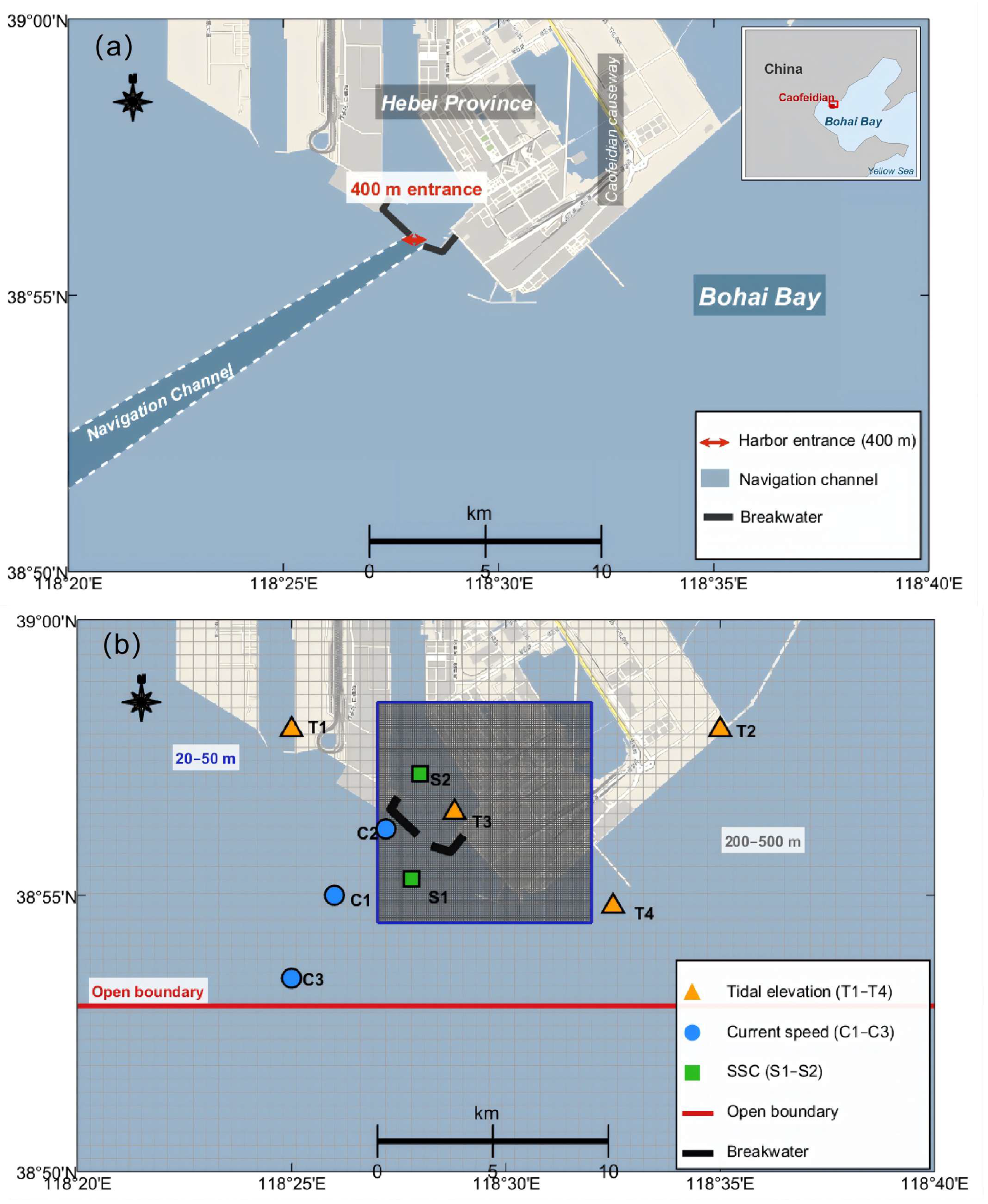
Caofeidian Port is located on the northern coast of Bohai Bay (38°50′–39°00′ N, 118°20′–118°40′ E), approximately 80 km south of Tangshan City, Hebei Province. The headland extends approximately 18 km seaward from the original coastline, with a natural deep channel maintained by tidal currents along its southern flank at depths of 20–25 m—anomalously deep for a bay averaging 18 m. The tidal regime is semi-diurnal with a mean spring tidal range of 2.4 m and neap range of 1.2 m. Tidal currents are strongly rectilinear along the main channel, with depth-averaged velocities reaching 0.76–0.84 m s−1 in the navigation channel during spring tides and peaking at 1.24 m s−1 at the headland tip based on field observations [8,10]. The system exhibits pronounced ebb dominance: ebb velocities exceed flood by approximately 10%, attributable to the asymmetric coastal geometry and the phase relationship between the M2 and M4 tidal constituents [9].
The outer harbor is enclosed by rubble-mound breakwaters approximately 6.5 km in total length, with a current entrance opening of 400 m oriented roughly perpendicular to the dominant tidal current axis, enclosing a basin area of approximately 12 km2. Bed sediment throughout the study domain is predominantly fine silt with median grain size d50 ≈ 0.063 mm, consistent with the fine-grained cohesive sediment environment documented across Bohai Bay. This grain size (d50 ≈ 0.063 mm) places the seabed sediment at the transition between non-cohesive and cohesive erosion regimes. Annular flume experiments on natural sand–silt mixtures from comparable Chinese silty coasts report critical erosion shear stresses of 0.21–0.42 Pa for silt contents ranging from 30% to 60% [21], consistent with the τ c e = 0.22 Pa adopted in this study (Section 2.2) and with the range 0.05–0.30 Pa reported for freshly deposited cohesive sediments [22,23]. The fine silt fraction is prone to flocculation, resulting in effective settling velocities substantially below single-grain Stokes estimates—a behavior that directly governs the residence time of suspended material within a partially enclosed harbor basin and thus the trap efficiency for tidally imported sediment.
The wave climate in Bohai Bay is governed by the East Asian monsoon system. A 40-year TOMAWAC hindcast (1979–2018) documents a mean annual significant wave height of less than 1.0 m across the Bohai Sea, with mean wave periods of 3–4 s in the central basin decreasing to less than 3 s near the coast. Seasonal variation is pronounced, with maximum Hs exceeding 1.5 m during winter cold-front events and minimum values below 0.5 m in summer [24]. Suspended sediment concentration exhibits corresponding seasonality: multi-year MODIS remote sensing (2003–2014) reveals that sea-surface SSC in the Bohai Sea is highest during winter–spring—when monsoon-driven wind-wave resuspension is strongest—and lowest during summer–autumn, with a seasonal amplitude averaging approximately 8 mg L−1 [25]. The August 2022 validation campaign (Section 2.3) thus corresponds to the lower end of the annual SSC range, and the offshore boundary SSC values adopted in this study (0.088 kg m−3 spring tide and 0.051 kg m−3 neap tide) represent summer conditions rather than annual maxima. Wave effects on bed shear stress are not coupled in the present tidal-only simulation—the consequences of this omission are quantified in Section 4.
Bathymetric data were digitized from the most recent nautical chart issued by the Maritime Safety Administration of China and supplemented by multibeam swath bathymetry surveys conducted in August 2022 within approximately 5 km of the breakwaters. All depth data were referenced to Chart Datum and converted to the WGS-84 coordinate system prior to model implementation. Sedimentation is a recognized operational concern at Caofeidian and comparable Bohai Bay deep-water ports. Converting the modeled net sediment import (Section 3.4) to an annual sedimentation volume—using a typical loose cohesive deposit dry density of ~1300 kg m−3—yields ~5.5 × 10⁶ m3 yr−1, which falls within the 3–8 × 10⁶ m3 yr−1 range reported in publicly available maintenance dredging records for comparable northern Chinese cohesive sediment deep-water ports [9,10]. This order-of-magnitude consistency confirms that harbor siltation constitutes a quantitatively significant engineering issue at this site. Site-specific dredging records for Caofeidian were not available for direct comparison and are identified as a priority for future validation. The geographic setting and computational grid are presented in Figure 1.

2.2. Hydrodynamic and Sediment Transport Model

Three-dimensional flow was simulated using Delft3D-FLOW (Delft3D 4 Suite, version 4.04.02; Deltares, Delft, The Netherlands; available at https://oss.deltares.nl/web/delft3d, accessed on 15 March 2026), which solves the Reynolds-averaged Navier–Stokes equations under the hydrostatic pressure and Boussinesq approximations [26]. The standard governing equations (free-surface continuity, horizontal momentum, and variable definitions) are provided in Appendix A.
A fully three-dimensional formulation is adopted because depth-averaged models cannot resolve the 18–31% surface-to-bed velocity shear or the vertical concentration of vortex vorticity—with bed-layer values attenuated to 41–48% of surface values—that the present results (Section 3.1 and Section 3.2) identify as essential to diagnosing tip-vortex sediment recirculation and vertical SSC stratification within the harbor basin. The vertical coordinate employs ten σ-layers with three layers concentrated near the bed to resolve the turbulent bottom boundary layer. Horizontal grid resolution ranges from 20 to 50 m in the near-field breakwater zone to 200–500 m in the far field. Manning roughness coefficient n = 0.018 m−1/3 s, and the computational time step is 60 s.
Vertical turbulent closure uses the standard k–ε scheme [27] with closure constants c1ε = 1.44, c2ε = 1.92, σk = 1.0, and σε = 1.3 (equations and variable definitions in Appendix A). This barotropic configuration resolves vertical velocity shear through the turbulent bottom boundary layer structure but does not include temperature or salinity transport. All vertical flow structures described in this study arise from bed friction and tidal forcing alone.
Suspended sediment transport is governed by the standard three-dimensional advection–diffusion equation implemented in Delft3D (equations and variable definitions in Appendix A).
Bed–water exchange follows the Partheniades–Krone formulation [28,29] (equations in Appendix A). Following standard Delft3D practice for fine cohesive sediments of this grain size class and the calibration against August 2022 field data, τ c e = 0.22 Pa and τ c d = 0.10 Pa were adopted.
Bed sediment in the study area is dominated by fine silt (d50 ≈ 0.063 mm). The near-bed suspended fraction is enriched in clay minerals and the finest silt fraction (<0.03 mm) relative to the bulk substrate, and this population is prone to flocculation. Following calibration, an effective settling velocity of w s = 0.3 mm s−1 was adopted—substantially below the Stokes velocity for bulk d50 grains (~0.9 mm s−1), consistent with the retardation associated with loose floc structures [30,31].
Open boundary tidal forcing comprises four major astronomical constituents (M2, S2, O1, and K1) with harmonic constants extracted from the TPXO 9.0 global tidal inversion model [32]. Offshore background SSC at the open boundary was specified as 0.088 kg m−3 during spring tides and 0.051 kg m−3 during neap tides, derived from field observations in the outer Bohai Bay.
Harbor water exchange was quantified using a conservative passive tracer module. Initial tracer concentration inside the harbor was set to 1.0 with 0.0 in the open sea. The daily water exchange rate was defined by the fractional tracer concentration decay within the harbor basin averaged over successive tidal cycles. This approach avoids ambiguities inherent in kinematic flushing time estimates and enables direct cross-scenario comparison at identical forcing conditions. A complete summary of model configuration parameters is provided in Table 1.

2.3. Model Validation

Model performance was evaluated against a 15-day continuous hydrographic survey conducted in August 2022, spanning one complete spring–neap tidal cycle. Tidal elevation was validated at four pressure-gauge stations (RBR virtuoso, RBR Ltd., Ottawa, ON, Canada; T1–T4), current speed and direction at three moored ADCP stations (Teledyne RDI Workhorse Sentinel 600 kHz, Teledyne RD Instruments, Poway, CA, USA; C1–C3) providing multi-layer velocity profiles, and SSC at two Van Dorn sampler stations (Beta™ 1920-H65, Wildlife Supply Company [Wildco], Yulee, FL, USA; S1–S2).
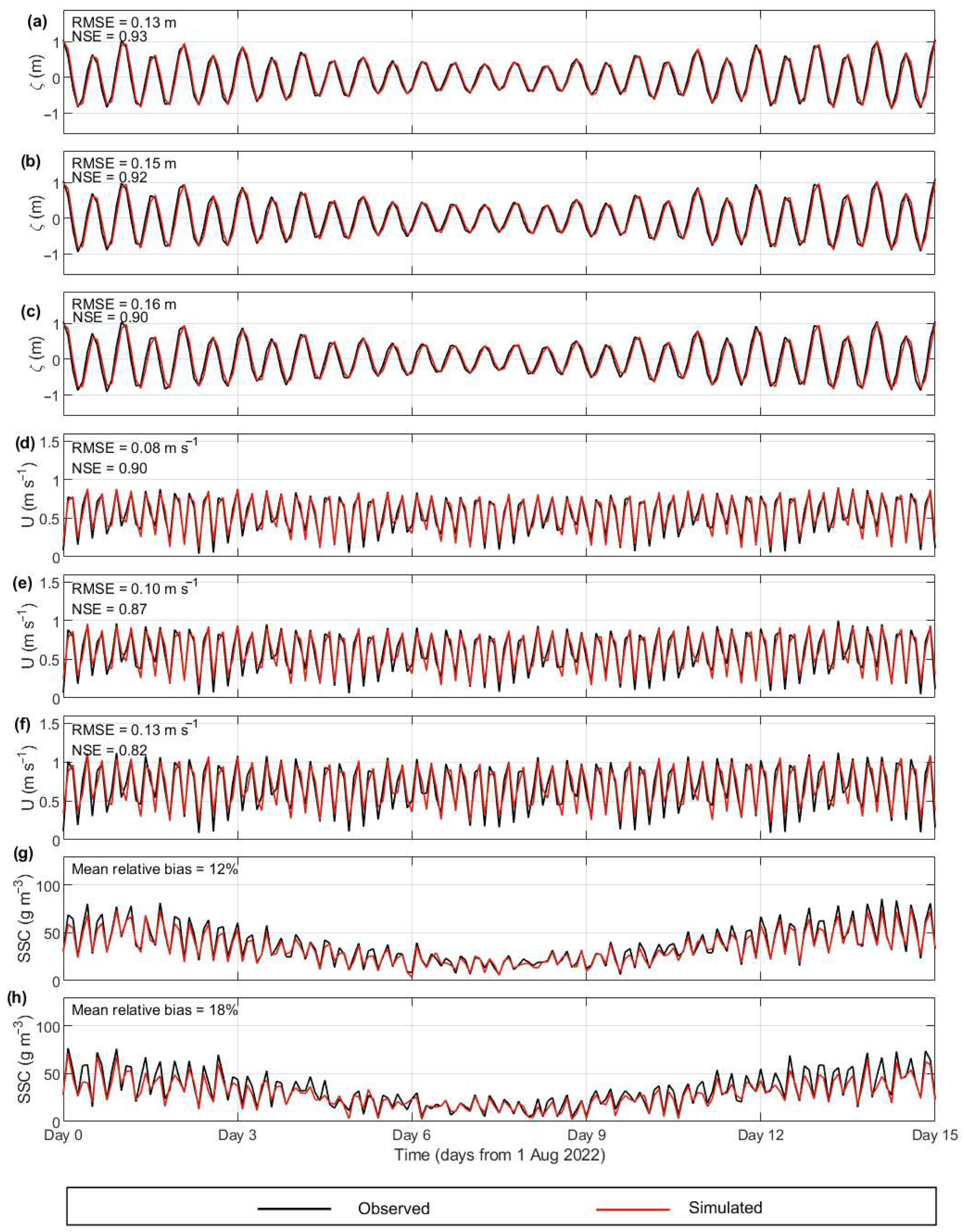
Tidal elevation predictions at T1–T4 yield RMSE values of 0.13–0.16 m with Nash–Sutcliffe efficiency (NSE) coefficients of 0.90–0.93, confirming accurate reproduction of tidal phase and amplitude across both spring and neap conditions. Depth-averaged current speed at C1–C3 yields RMSE = 0.08–0.13 m s−1 and NSE = 0.82–0.90. Flow direction accuracy is assessed by decomposing velocity into u and v components separately—a more robust approach than applying NSE directly to circular directional data—giving component NSE of 0.83–0.89 (u) and 0.79–0.86 (v) with directional RMSE of 23–36°. Larger errors occur near slack water, where small residual velocities make direction sensitive to minor speed errors. Surface SSC at S1 shows a mean relative bias of approximately 12%; at S2, approximately 18%. Both stations show a systematic low bias in bottom-layer SSC during high-velocity periods, attributable to the absence of wave orbital velocity contributions to composite bed shear stress in this tidal-only simulation—a limitation addressed in Section 4.
Validation results are shown in Figure 2. Overall agreement between observations and simulations is sufficient to resolve the tidal-scale hydrodynamic and sediment processes that are the focus of this study, and the bias characteristics are consistent with those reported for comparable Delft3D coastal applications [33].
The August 2022 validation campaign was deliberately selected as a stringent test of model performance: the boreal summer in Bohai Bay coincides with elevated suspended sediment concentrations, the active East Asian summer monsoon, and the seasonal peak in mean wave climate [24,25], representing the most demanding period for a tidal-only configuration. The 15-day campaign captures one complete spring–neap cycle, ensuring representativeness of the dominant tidal forcing structure. Multi-season validation—particularly under winter cold-front conditions and energetic wave events—would further constrain model robustness and is identified as a priority for follow-up work.
The systematic underestimation of bottom-layer SSC (~18% at S2) during high-velocity periods warrants specific attention because near-bed processes control erosion, deposition, and net sediment flux. This bias is attributed to the absence of wave-enhanced bed shear stress in the present tidal-only simulation. Wave orbital velocities augment the composite bed shear stress above the tidal-only value, an effect that is most consequential in the near-entrance zone where τ_b hovers near the critical erosion threshold (Section 3.3). The implications of this bias for net sediment flux estimation are quantified through a correction analysis in Section 3.4, and the resulting uncertainty bounds are incorporated into the Discussion (Section 4).

2.4. Scenario Design

Five scenarios were constructed to isolate the effects of breakwater presence and entrance geometry (Table 2). Scenario ① (no breakwater) provides the pre-construction hydrodynamic baseline. Scenario ② (Plan A, 400 m entrance) represents the current operational configuration. Scenarios ③ (Plan B, 300 m), ④ (Plan D, 250 m), and ⑤ (Plan C, 200 m) test entrance width sensitivity with breakwater alignment and total enclosed area held constant. Plan D was added during revision to refine the hydraulic transition interval initially identified between Plans B and C. All simulations ran for 30 days. The first 15 days served as spin-up and analyses were conducted on the stabilized Days 15–30. Spring and neap tidal cycle results were extracted from representative cycles centered on Days 21–22 and Days 27–28, respectively. Water exchange rates were computed from the full 30-day tracer simulation.

3. Results

3.1. Breakwater Effects on Near-Field Velocity Structure

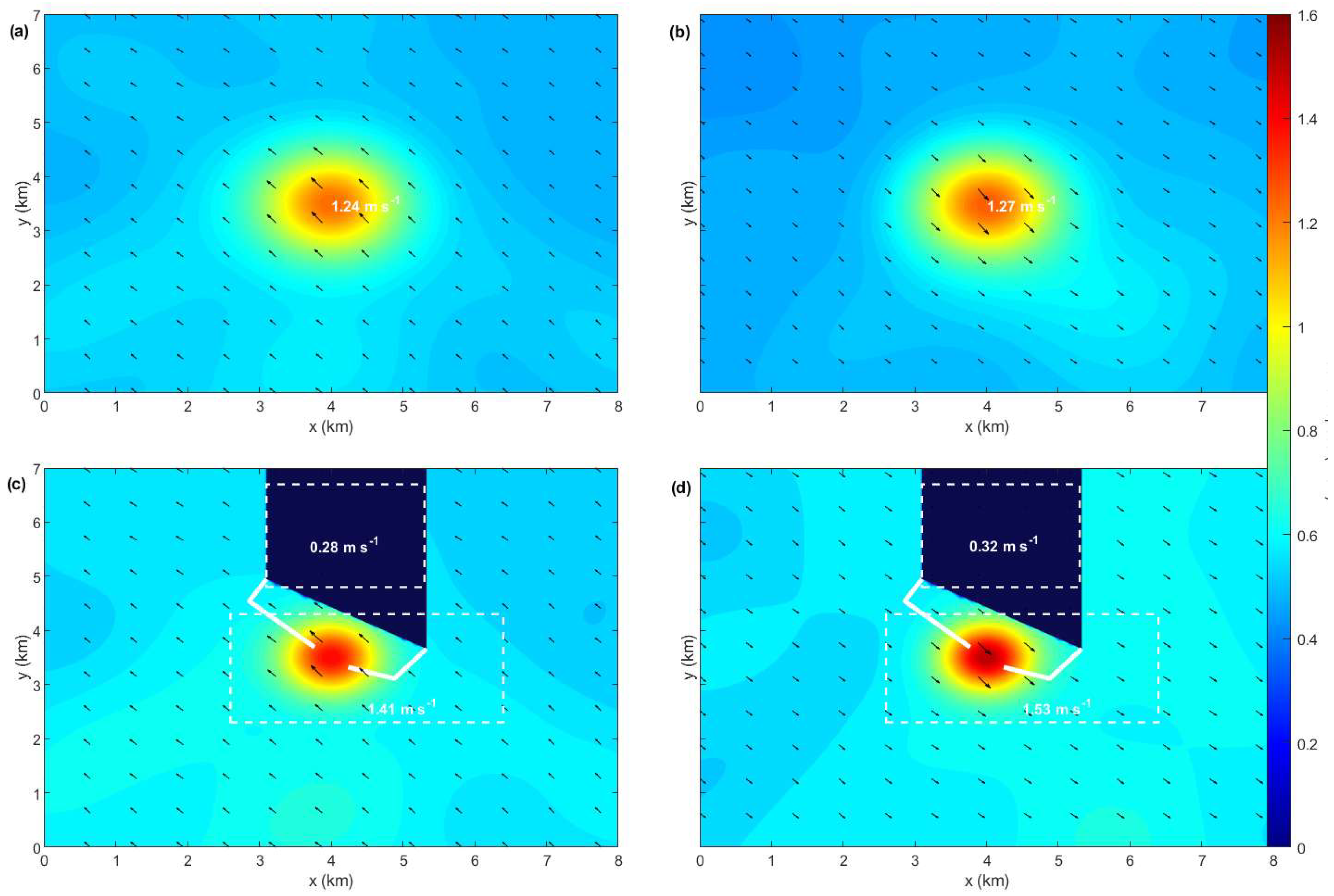
Under pre-breakwater conditions (Scenario ①), the main navigational channel sustains depth-averaged velocities of 0.76 m s−1 during flood and 0.84 m s−1 during ebb at spring tide—an ebb-to-flood ratio of approximately 1.1, confirming the ebb-dominant character of the Caofeidian headland flow. The simulated headland tip velocity reaches 1.27 m s−1 during peak ebb, in close agreement with the field-observed maximum of 1.24 m s−1, and the small residual difference is within the expected range of grid interpolation and timing window averaging effects.
The enclosing breakwaters (Scenario ②) fundamentally restructure this pattern. Inside the harbor basin, depth-averaged velocity during spring tides is reduced to 0.28 m s−1 (flood) and 0.32 m s−1 (ebb), representing decreases of 63.2% and 61.9% from Scenario ①, respectively. This reduction is not spatially uniform. Within approximately 500 m of the entrance opening, the velocity reduction is only about 38%—the tidal jet penetrates well into the harbor interior, sustaining a residual dynamic zone where bed shear stresses remain above the critical erosion threshold (Section 3.3). Moving toward the harbor interior, the reduction reaches approximately 71%, creating a pronounced energy gradient along the harbor axis that directly determines the sedimentation pattern described in Section 3.4.
At the breakwater tips, the velocity field reverses this trend entirely. Flow constriction through the 400 m entrance generates a jet that exceeds pre-construction background velocities: the eastern tip reaches 1.41 m s−1 during flood and 1.53 m s−1 during ebb—increases of 14% and 18% above Scenario ① values. Both values exceed the pre-construction headland maximum of 1.27 m s−1, indicating that the breakwater introduces a new scour intensity zone that does not exist in the pre-construction velocity record. The larger ebb-phase enhancement (18% vs. 14% for flood) reflects the favorable geometry of the seaward breakwater face for ebb approach flow alignment combined with the ebb-dominant background forcing.
Vertical structure adds a third dimension to this differentiation. Surface-layer velocities (σ = 0.1) exceed near-bed values (σ = 0.9) by 18–31% throughout the tidal cycle, a gradient produced by the no-slip bottom boundary condition and the logarithmic turbulent boundary layer profile resolved by the near-bed σ-layer refinement. The surface–bottom velocity differential is larger during flood (31%) than during ebb (18%). During flood, tidal acceleration is concentrated in the surface layers as the boundary layer adjusts to the accelerating flow, producing steeper vertical shear; during ebb, the decelerating flow allows turbulent mixing to redistribute momentum more uniformly across the water column, reducing the vertical gradient. This tidal-phase modulation of vertical shear is a consequence of the boundary layer development cycle and has direct implications for interpreting depth-averaged model outputs: the surface-intensified structure of the flood entrance jet governs the vertical distribution of suspended sediment import, as discussed in Section 3.4.
These three dynamically distinct sub-environments—accelerated headland jet zone, transitional near-entrance zone, and quiescent depositional interior—are clearly expressed in both flood and ebb phases, as shown in Figure 3. The gradient between the near-entrance and interior zones is steeper during ebb than flood, consistent with the stronger ebb jet organizing the transition zone over a shorter spatial length scale.
The velocity reduction from 71% in the harbor interior to 38% near the entrance represents a gradient that governs both the spatial extent of active bed erosion and the trap efficiency of the harbor for suspended fine sediment. A harbor entrance that creates a sharp rather than gradual velocity transition would allow a larger proportion of flood-imported sediment to penetrate the depositional interior before ebb reversal—the spatial form of this gradient is, therefore, as important as the magnitude of the mean reduction.

3.2. Vorticity Structure and Three-Dimensional Flow Features

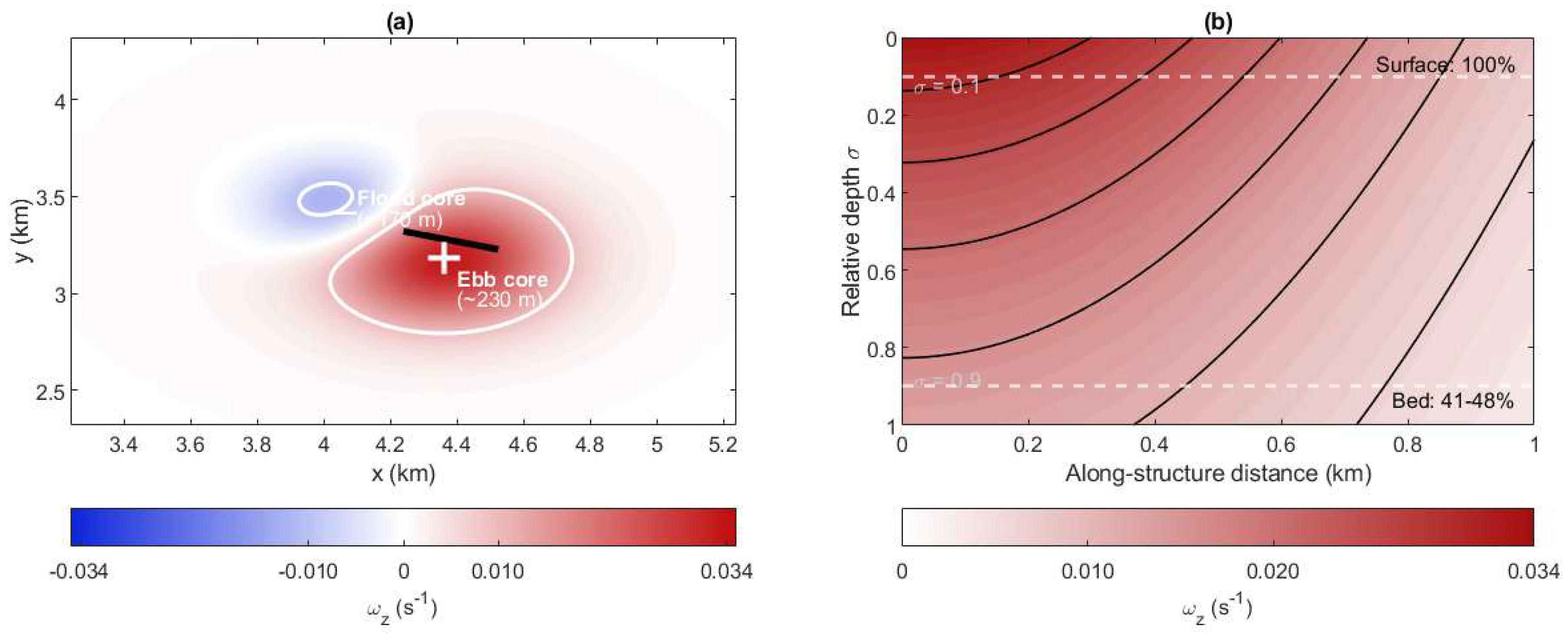
Flow separation at the eastern breakwater head generates a persistent tip-vortex system with markedly different properties between flood and ebb. During flood, a clockwise vortex forms on the lee side of the eastern tip with a core radius of approximately 170 m, peak vertical vorticity of 0.021 s−1, and persistence of approximately 3.4 h. During ebb, the counterclockwise ebb vortex attains a core radius of approximately 230 m, peak vorticity of 0.034 s−1, and persists for approximately 4.6 h. The ebb vortex is approximately 34% larger in radius and 62% more intense than its flood counterpart.
This asymmetry exceeds what the modest ebb–flood velocity ratio (~1.1) would predict from simple kinematic scaling. Three factors cooperate: the longer ebb duration in this semi-diurnal ebb-dominant system, the more favorable alignment of the ebb approach flow with the breakwater axis over a longer separation length on the seaward face, and the greater effective vortex development distance on the seaward side compared with harbor-side separation during flood. The persistence difference—4.6 h ebb versus 3.4 h flood—is consequential for sediment transport because it determines how long each vortex entrains and recirculates near-bed material before destruction by the subsequent tidal-phase reversal.
Vertically, the vortex is concentrated in the upper and middle water columns. Bottom-layer vorticity (σ = 0.9) is only 41–48% of the surface-layer value, with the steepest attenuation within the lowest two σ-layers where bed friction suppresses rotational motion. The vortex-driven lateral transport of suspended sediment is thus surface intensified, which partly explains why bottom-mounted instruments at the eastern tip systematically underestimate the full sediment recirculation flux.
The western breakwater head behaves differently. During flood, returning harbor recirculation interferes with the external approach flow, preventing stable vortex attachment; during ebb, a coherent vortex forms with radius ~180 m and intensity ~0.019 s−1, but persistence of only ~2.8 h—substantially less than the eastern counterpart. This east–west asymmetry is a product of the non-symmetric harbor plan geometry rather than any structural difference between the breakwaters, and it means that the eastern tip is the dominant site of vortex-driven scour and sediment recirculation.
The vorticity structure and its vertical decay are illustrated in Figure 4. The surface-to-bed attenuation factor of approximately two to three means that assessment of near-field scour based solely on depth-averaged velocity or bed shear stress will miss the upper water column vortex dynamics that govern sediment recirculation.

3.3. Bed Shear Stress Distribution and Critical Threshold Analysis

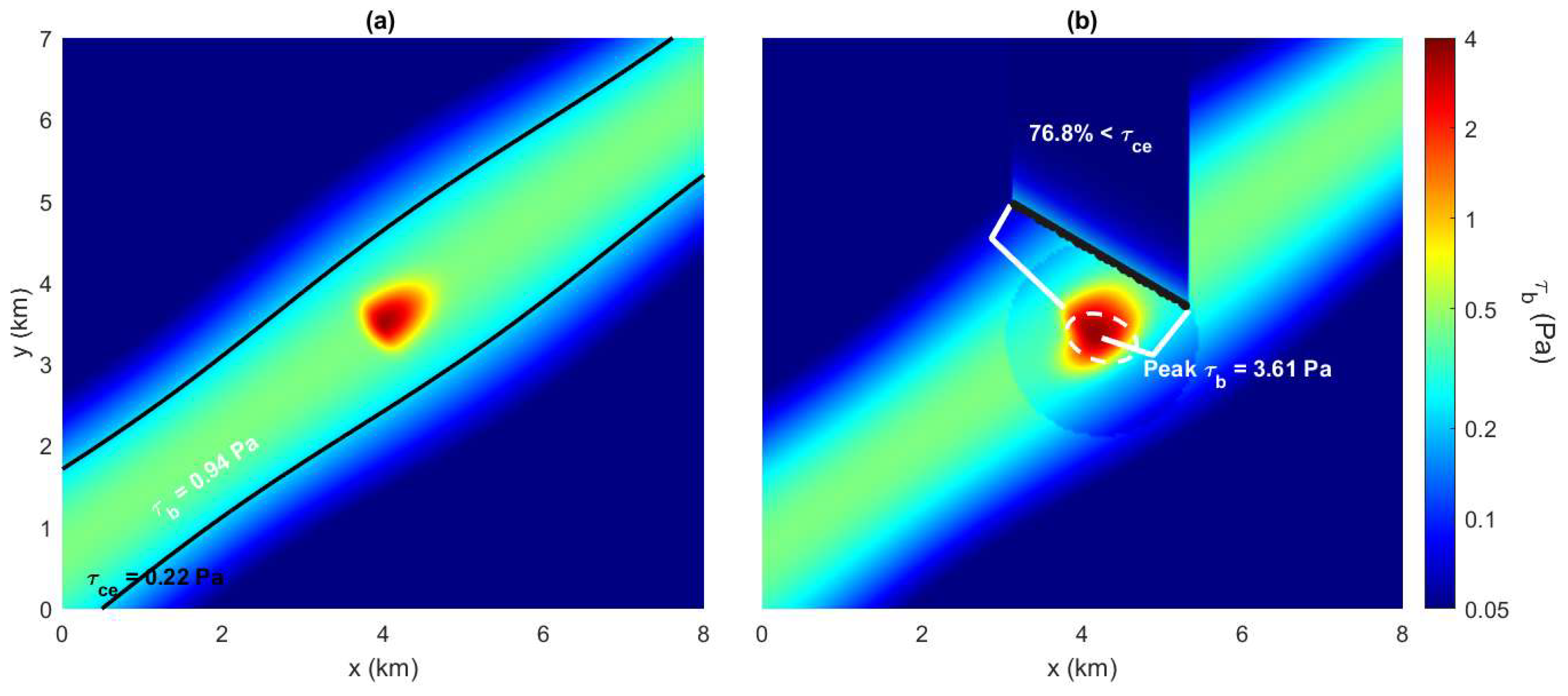
Before breakwater construction, the spring-tide tidal-mean bed shear stress in the main channel is τ b = 0.94 Pa, with instantaneous peak values at the headland tip reaching 3.38 Pa. Both values substantially exceed τ c e = 0.22 Pa, confirming that the pre-construction seabed in the main channel was in persistent active resuspension throughout most of the tidal cycle.
The breakwater’s most consequential effect on harbor sedimentation potential is the collapse of bed shear stress below τ c e across most of the basin. Under Scenario ②, the spring-tide tidal-mean τ b averaged over the harbor area falls to 0.17 Pa—a decrease of 81.9%. Applying τ c e = 0.22 Pa as the criterion separating depositional from erosional bed states, 76.8% of the harbor area falls below this threshold during spring tides, rising to 91.3% during neap tides. The sub-threshold depositional zone dominates the harbor interior, while the supra-threshold zone is confined to within approximately 500 m of the entrance, where the tidal jet maintains τ b of 0.25–0.45 Pa.
At the breakwater tips, the local bed shear stress is intensified. The eastern tip reaches a peak ebb-phase τ b of 3.61 Pa—exceeding the pre-construction headland maximum of 3.38 Pa—because flow concentration through the constricted aperture generates higher local velocities than the unconstricted headland flow. The pre-construction velocity record is, therefore, not a conservative design bound for armor stone stability at the breakwater toe. Even at slack water, residual near-bed turbulence maintains τ b above approximately 0.10 Pa in the near-entrance throat, preventing the complete settling quiescence that characterizes the harbor interior, where slack-water τ b falls to 0.03–0.06 Pa.
This spatial bifurcation is illustrated in Figure 5. The τ c e = 0.22 Pa contour line maps the boundary within which maintenance dredging is most likely to be cost-effective: sediment deposited in the interior accumulates without self-cleaning, while near-entrance deposits cycle repeatedly without net export.
The boundary between the two regimes shifts between spring and neap tides—from approximately 500 m to approximately 300 m penetration of the supra-threshold zone—but the qualitative bifurcation persists throughout the spring–neap cycle, making it a reliable structural feature of the harbor sedimentation regime under the current 400 m entrance configuration.
Because the spatial extent of the depositional zone depends directly on the adopted critical erosion threshold, a parameter sensitivity analysis was conducted by perturbing the three most influential sediment transport parameters independently while holding the simulated velocity and shear stress fields unchanged (Table 3). The critical erosion shear stress τ c e was varied by ±20% (0.176–0.264 Pa), spanning the experimental range reported for natural sand–silt mixtures with d50 in the 0.05–0.08 mm class [21,22]. The effective settling velocity w_s was varied by ±20% (0.24–0.36 mm s−1), reflecting the uncertainty associated with flocculation-dependent settling in fine cohesive environments. The Manning roughness coefficient n was varied by ±10% (0.016–0.020), propagated to the shear stress field via the τ b ∝ n2 relationship. Results show that the depositional area fraction is most sensitive to τ c e (70.2–82.4%), followed by n (73.1–80.2%), with w_s exerting only an indirect influence through deposition flux (±1.5 percentage points). The root-sum-square composite uncertainty yields a robust range of 68–83% for the depositional area fraction and 8.8–11.0 × 10⁶ kg per cycle for the spring–neap weighted-mean net sediment flux. These parameter sensitivity bounds do not include the additional effect of wave-enhanced bed shear stress, which is assessed separately in Section 4.

3.4. SSC Distribution and Net Sediment Flux

The bed shear stress regime described above maps directly onto the SSC field. Under Scenario ②, the spring-tide tidal-mean SSC in the harbor basin decreases from 0.078 kg m−3 (Scenario ①) to 0.037 kg m−3—a reduction of 52.6%. During neap tides, the corresponding decrease is from 0.039 to 0.024 kg m−3, a reduction of 39.1%. The smaller percentage reduction during neap tides is physically interpretable: lower offshore SSC (0.051 vs. 0.088 kg m−3) weakens the concentration gradient across the entrance, reducing the diffusive component of sediment import, while the lower tidal energy simultaneously reduces internal resuspension in both scenarios.
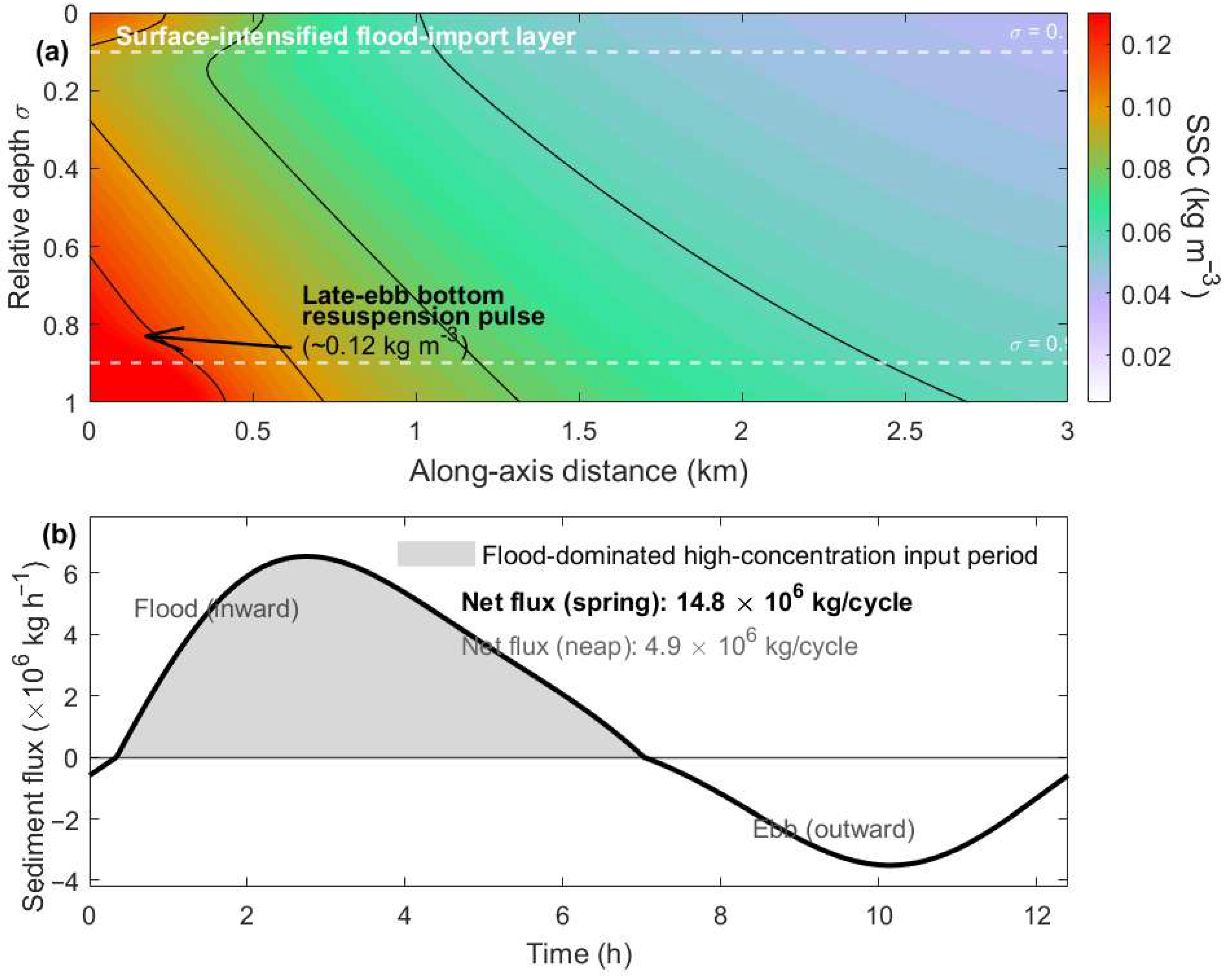
Vertical SSC stratification within the harbor is pronounced. Bottom-layer concentrations (σ = 0.9) exceed surface values by 37–64% when averaged over the tidal cycle, driven by gravitational settling of suspended material toward the bed between periods of active resuspension. The flood–ebb asymmetry in this ratio—smallest during flood, largest during ebb—reflects the surface-intensified structure of the flood entrance jet, which carries high-SSC open-sea water into the upper water column before it settles and mixes downward. The most dynamically distinct feature is the late-ebb near-bed resuspension pulse: as ebb velocities decelerate in the near-entrance zone, the bed shear stress passes through τ c e and previously deposited near-bed material is briefly mobilized, creating a concentrated pulse of approximately 0.12 kg m−3—roughly three times the depth-averaged harbor mean—that persists for approximately 1.2 h before re-settling as velocities approach slack. This feature corresponds precisely to the supra-critical shear stress area identified in Section 3.3 and is visible in the upper panel of Figure 6.
Net sediment flux through the 400 m entrance is directed into the harbor throughout the simulation—the harbor is in continuous net accretion. The driving mechanism is asymmetric tidal pumping. During flood, the incoming current carries open-sea water at a spring-tide boundary SSC of 0.088 kg m−3; during ebb, although ebb velocities are slightly higher, the harbor SSC has been reduced by settling during the preceding slack water to approximately 0.032–0.041 kg m−3, so the outgoing sediment flux is smaller than the incoming flood flux despite the ebb velocity advantage. The velocity–concentration phase relationship biases net transport toward the harbor interior regardless of the system’s ebb-dominant velocity character. Spring-tide net import amounts to 14.8 × 10⁶ kg per tidal cycle (near-bed-corrected upper bound: 16.4–16.5 × 10⁶ kg per cycle; wave-coupled upper bound: 17.8–19.2 × 10⁶ kg per cycle), and neap-tide net import is 4.9 × 10⁶ kg per cycle (near-bed-corrected: 5.4–5.5 × 10⁶ kg per cycle). A spring–neap weighted mean gives approximately 9.9 × 10⁶ kg per tidal cycle (parameter sensitivity range: 8.8–11.0 × 10⁶ kg per cycle; upper bound including near-bed SSC bias correction and literature-informed wave-coupling estimate: 13–14 × 106 kg per cycle)—a magnitude consistent with the severe siltation conditions known to affect fine-sediment harbor basins in Bohai Bay. The derivation of these uncertainty bounds is detailed in Section 3.5 and Section 4.
Entrance width sensitivity reveals a nonlinear trade-off summarized in Table 4. Reducing the entrance from 400 m (Plan A) to 300 m (Plan B) decreases spring-tide net sediment flux by 21.0% while reducing the harbor daily water exchange rate by only 17.1%: the marginal efficiency ratio (flux reduction per unit exchange loss) is approximately 1.23, meaning sedimentation control outpaces water quality degradation. The further reduction to 200 m (Plan C) delivers an additional 20.9 percentage points of flux reduction (total −41.9% from Plan A) at the cost of an additional 20.6 percentage point drop in water exchange rate (total −37.7%), giving a marginal efficiency ratio of approximately 1.01. This step change in efficiency between the A → B and B → C transitions indicates the onset of hydraulic choking behavior below ~300 m, with the harbor becoming increasingly decoupled from external tidal forcing. To refine the transition interval, an intermediate 250 m scenario (Plan D; detailed results in Appendix B) was conducted. Plan D yields a step marginal efficiency ratio of 1.03 for the B → D transition, declining to 1.01 for D → C (Table 4). The monotonic decline across Plans A → B → D → C (1.23 → 1.03 → 1.01) localizes the onset of hydraulic choking to the 250–300 m range, narrowing the previously identified 200–300 m interval by half. Precise identification of a point optimum within this 50 m range requires further scenario refinement and explicit water quality transport modeling, which are identified as follow-up priorities.

3.5. Reynolds Flux Decomposition at the Harbor Entrance

To isolate the physical mechanisms responsible for net sediment import, a Reynolds flux decomposition was applied to the entrance cross-section of Scenario ② during the representative spring-tide cycle (Days 21–22). At each grid point across the 400 m opening and through the 10 σ-layers, the instantaneous normal velocity u and suspended sediment concentration c were decomposed into tidal-cycle means (ū, c ¯ ) and fluctuations (u’, c’), and the net flux integrated over the cross-section and tidal period was partitioned as:
F n e t = u ¯ c ¯   d A   d T F a d v + u c ¯   d A   d T F p u m p
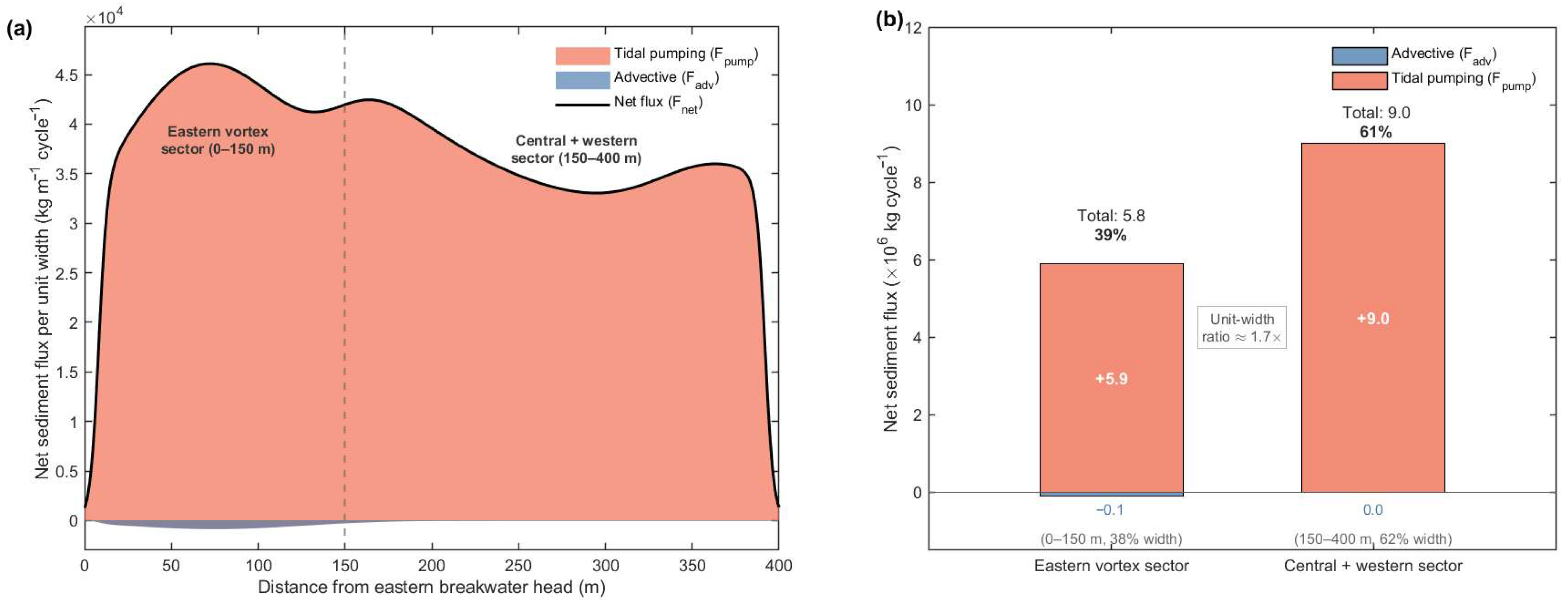
The advective component (Fadv) contributes only −0.1 × 10⁶ kg per cycle (−0.7% of net flux), representing a weak net export consistent with the system’s ebb-dominant velocity character. The tidal pumping component (Fpump) contributes +14.9 × 10⁶ kg per cycle (100.7%), confirming that net sediment import is driven entirely by the phase relationship between tidal velocity and SSC rather than by mean residual transport.
Lateral partitioning of the entrance cross-section further reveals the role of the eastern tip vortex. The entrance was divided into an eastern tip-vortex influence sector (0–150 m from the eastern breakwater head, corresponding to ~38% of the total opening width) and a central + western sector (150–400 m). The eastern vortex sector contributes 5.8 × 10⁶ kg per cycle—39% of the total net import—despite occupying only 38% of the entrance width. The unit-width flux through the vortex sector is approximately 1.7 times that of the central + western sector (Figure 7). This disproportionate contribution provides direct quantitative evidence that vortex-assisted recirculation constitutes an independent sediment transport mechanism that enhances tidal pumping import beyond what the cross-sectionally uniform flow field would produce. The advective component within the vortex sector is −0.1 × 10⁶ kg per cycle, confirming that even locally, the net import is attributable to pumping rather than mean-flow advection.
As documented in Section 2.3, the model systematically underestimates bottom-layer SSC by approximately 18% during high-velocity periods owing to the absence of wave-enhanced bed shear stress. Because the bottom three σ-layers (σ = 0.7–0.9) contribute approximately 55–65% of total cross-sectional sediment flux—reflecting the 37–64% bottom-layer SSC enrichment over surface values reported in Section 3.4—a bias correction was applied by scaling near-bed SSC upward by 18% in the bottom three layers, with a linear taper to 9% in the middle layers and no correction in the upper layers. This correction yields a spring-tide net flux of 16.4–16.5 × 10⁶ kg per cycle and a spring–neap weighted mean of 10.9–11.1 × 10⁶ kg per cycle—an increase of 10–12% over the uncorrected baseline. This near-bed correction represents the minimum upward adjustment attributable to the identified model bias. The additional effect of wave-enhanced resuspension, which would further increase both bed shear stress and near-bed SSC, is assessed using literature-informed bounds in Section 4.

4. Discussion

The results establish a coherent mechanistic chain from breakwater geometry to harbor sedimentation: flow constriction at the entrance → asymmetric tip-vortex formation → redistribution of bed shear stress below the critical threshold across 76.8% of the harbor area (sensitivity range 68–83%; wave-coupled lower bound ~60%) → spatially bifurcated deposition and resuspension regimes → net tidal pumping import at ~9.9 × 10⁶ kg per cycle (sensitivity range 8.8–11.0; wave-coupled upper bound ~13–14; spring–neap weighted mean). Each link connects to the broader literature on tidal inlet and harbor dynamics, and several aspects of the Caofeidian result depart from behavior expected in simpler systems.
The 34% larger radius and 62% greater intensity of the ebb vortex relative to the flood vortex exceed what the modest ebb–flood velocity ratio (~1.1) would predict from isotropic vortex scaling. Research on headland-associated vortex systems confirms that vortex asymmetry in ebb-dominant settings arises primarily from the longer approach length and greater effective separation distance on the lee side during ebb, independent of velocity magnitude per se [34,35]. At Caofeidian, the additional geometric asymmetry between the seaward (ebb-facing) and harbor-side (flood-facing) surfaces of the breakwater amplifies this tendency beyond what headland geometry alone would produce. The consequence for sediment transport is not simply that the ebb vortex is larger—it is that the ebb vortex persists long enough (4.6 h) to entrain sediment from the near-bed resuspension layer seaward of the entrance and recirculate it toward the harbor before the subsequent flood. Flux decomposition (Section 3.5, Figure 7) demonstrates that the eastern tip-vortex sector contributes ~39% of net entrance flux at a unit-width rate ~1.7 times that of the central sector, while the advective component is effectively zero (−0.7%). This quantitatively isolates vortex-assisted recirculation from passive tidal pumping and resolves the causal ambiguity inherent in earlier flux-magnitude-only diagnostics. This vortex-assisted recirculation adds to the purely advective tidal pumping flux and explains why the harbor accumulates sediment net despite ebb-dominant velocities. Analogous vortex-enhanced import has been documented in groyne field studies, where gyre structures trap fine sediment at rates that depth-averaged velocity fields substantially underpredict [36].
The spatial structure of bed shear stress—resuspension-active near-entrance zone versus permanently depositional interior—has direct maintenance implications beyond simple dredging volume estimates. The near-entrance zone undergoes cycling of resuspension and re-deposition at each tidal cycle without net export: ebb-phase mobilization releases material to the water column, but the declining concentration gradient during ebb prevents efficient outward transport before the subsequent flood re-imports open-sea sediment. This differs fundamentally from the harbor interior, where deposited sediment accumulates with negligible self-cleaning. Measurements of critical erosion shear stress in comparable cohesive tidal environments show that fine silt aggregates exhibit substantially lower τ c e when recently deposited and unconsolidated compared to aged, consolidated deposits [22,23]. The near-entrance sediment, being repeatedly disturbed and re-deposited, likely maintains lower bulk density and lower effective τ c e than consolidated interior deposits—which means the actual resuspension zone may be somewhat larger than our model estimates based on a fixed τ c e = 0.22 Pa. Field measurements using inertial dissipation methods in cohesive tidal environments further demonstrate that both τ b and settling velocity vary significantly with tidal phase and position at sub-kilometer scales [37], a spatial variability that time-averaged sedimentation assessments will systematically misrepresent.
The trade-off between sedimentation control and water exchange quality in the entrance width sensitivity analysis is consistent with hydraulic choking operative below approximately 300 m for this harbor geometry. Research on tidal-induced circulation in semi-enclosed harbor basins consistently finds that the water exchange rate responds disproportionately to entrance constriction below a critical width-to-basin-length ratio, with residence times increasing nonlinearly beyond this threshold [19,20]. The near-linear sedimentation response in the 300–400 m range versus the accelerating water quality cost in the 200–300 m range is consistent with this hydraulic transition. Analogous decoupling between sedimentation reduction and water renewal cost has been quantitatively characterized for harbor basin configurations enclosed by seawalls in wind-driven systems [38]. The marginal efficiency response declines monotonically across Plans B, D, and C (1.23 → 1.03 → 1.01), localizing the hydraulic transition to the 250–300 m entrance width range. Further refinement at 25 m increments within this 50 m interval would enable precise identification of a point optimum and explicit water quality transport modeling, since the acceptable residence time threshold depends on harbor use and regulatory context. This is identified as a priority for follow-up work.
The net sediment import of ~9.9 × 10⁶ kg per cycle (sensitivity range 8.8–11.0; wave-coupled upper bound ~13–14) implies substantial annual accretion, broadly consistent with maintenance dredging cycles reported for comparable meso-tidal fine-sediment harbor basins [39,40,41]. Converting this flux to an annual sedimentation volume yields ~5.5 × 10⁶ m3 yr−1 (assuming a loose cohesive deposit dry density of ~1300 kg m−3), consistent within an order of magnitude with publicly reported maintenance dredging volumes for comparable northern Chinese deep-water ports (3–8 × 10⁶ m3 yr−1 [9,10]). The flood-dominant concentration pumping mechanism driving this accretion is well-documented in tidal inlet literature: analysis of tidal channels with lateral bathymetric variation demonstrates that the concentration–velocity phase lag generates net landward flux in ebb-dominant systems whose velocity skewness alone would predict export [42], and the Caofeidian harbor represents this physics in a confined geometry, amplified by vortex recirculation.
The connection between these near-field results and bay-scale material transport deserves attention. Lagrangian flow network analysis showed that reclamation increased input entropy near the port by ~160%, interpreted as enhanced material aggregation capacity [7]. The near-field dynamics quantified here provide a specific mechanism: the breakwater-induced tip-vortex system converts the headland’s strong tidal energy from a dispersal agent into an aggregation driver, creating a concentrated material-capture zone at the harbor entrance. Bay-scale numerical studies confirm the nonlinear sensitivity of the Bohai Sea to coastal geometry changes [5], and reclamation-driven transitions from export-dominated to import-dominated sediment transport regimes have been documented in comparable embayments along the Chinese coast [43]. The bay-scale entropy measure integrates the cumulative consequence, and the near-field 3D simulation identifies the responsible physical processes.
Comparative assessment against other harbor siltation studies provides useful context. Delft3D modeling of harbor layout changes in the North Sea tidal environment showed that jetty reorientation reduces entrance area sedimentation by modifying approach flow alignment relative to the vortex separation angle [44]—implying that the fixed breakwater orientation at Caofeidian may not be geometrically optimal relative to the dominant ebb current direction. Simulation of a comparable Chinese port documented entrance velocity reductions of 40–60% and typhoon-induced deposition of 0.5–1.0 m at the harbor entrance [45]—magnitudes broadly consistent with the current findings, though the 3D vertical structure revealed here indicates that depth-averaged predictions would substantially misrepresent the near-bed deposit distribution. Delft3D-based suspended sediment budget analyses for fluvial-tidal systems confirm the robustness of Partheniades–Krone cohesive formulations over tidal timescales when effective settling velocity is calibrated against field data rather than single-grain Stokes estimates [46], validating the calibration approach adopted here.
Seven limitations constrain the scope of these findings. The most consequential is the absence of wave coupling. Surface wave orbital velocities augment the bed shear stress through nonlinear wave–current interaction, an effect that the present tidal-only configuration does not resolve. Based on published SWAN+Delft3D coupling studies in comparable shallow cohesive environments, near-bed bed shear stress under average Bohai Bay weather conditions (Hs ~ 0.8–1.2 m [24]) is enhanced by approximately 30–60% relative to tidal-only values [47]. Applying this literature-informed correction to the present results yields a robust lower bound of ~60% for the depositional area fraction (versus 76.8% in the tidal-only baseline) and a corresponding upper bound of 13–14 × 106 kg per tidal cycle for the spring–neap weighted-mean net sediment import (versus 9.9 × 10⁶ kg per cycle). These are literature-informed bounds rather than direct simulation outputs. Explicit wave–current coupled simulation is identified as the highest-priority methodological extension. Critically, even at these wave-corrected bounds, the qualitative conclusions of this study—predominantly depositional harbor interior, asymmetric tidal pumping import, vortex-assisted recirculation, and the 250–300 m hydraulic transition—remain robust. Second, the parameter sensitivity analysis (Section 3.3, Table 3) demonstrates that the depositional area fraction and net sediment flux are most sensitive to the adopted critical erosion threshold ( τ c e ± 20% shifts the depositional fraction by ±6 percentage points), followed by Manning roughness (±4 percentage points). Even the root-sum-square composite uncertainty (68–83% for area; 8.8–11.0 × 10⁶ kg per cycle for flux) does not alter the qualitative sedimentation pattern, but underscores the importance of site-specific erosion testing for future quantitative refinement. Third, although the addition of Plan D (250 m) narrows the hydraulic transition to the 250–300 m range, four entrance widths remain insufficient to identify a point optimum within this interval. Further refinement at 25 m increments (e.g., 260, 270, 280, and 290 m) would be needed to resolve the precise trade-off curve, and this is identified as a follow-up priority. Fourth, the standard k–ε turbulence closure may overestimate vertical mixing during neap tides when tidal stirring is weaker, potentially contributing to the ~18% SSC bias at S2 during neap periods. Finally, the predicted instability of the western breakwater tip vortex requires targeted field verification, as idealized bathymetry near the western root in this model may not capture the full complexity of the actual geometry. The single cohesive sediment class adopted here is supported by the narrow grain size distribution of the study area (d50 ≈ 0.063 mm, dominated by fine silt), under which a multi-fraction representation would yield only marginal refinement at the cost of additional poorly constrained parameters. Explicit multi-fraction modeling is contingent on site-specific grain size spectrum data and is identified as a refinement target for future work. Similarly, morphodynamic bed-level updating was deliberately not enabled because the 30-day simulation duration is well within the timescale over which morphological feedback on the hydrodynamic field is negligible for this harbor configuration. The present study targets diagnostic characterization of the transport mechanisms under the as-built geometry rather than long-term morphological evolution, the latter being identified as an independent follow-up investigation.

5. Conclusions

A three-dimensional tidal–sediment coupled Delft3D model applied at Caofeidian Port demonstrates that breakwater construction imposes a spatially differentiated velocity reduction of 61.9–63.2% in the harbor basin, with the near-entrance zone (within ~500 m of the opening) experiencing a velocity reduction of only approximately 38%—sufficient to maintain bed shear stress above the erosion threshold—while the deep interior reaches 71% reduction under predominantly depositional conditions. The eastern breakwater tip generates an ebb vortex (radius ~230 m; vorticity 0.034 s−1) approximately 34% larger and 62% more intense than the flood vortex (radius ~170 m; vorticity 0.021 s−1), an asymmetry that drives vortex-assisted sediment recirculation toward the harbor and sustains net sediment import despite the system’s ebb-dominant velocity character. Reynolds flux decomposition confirms that the eastern tip-vortex sector contributes ~39% of net sediment import (advective component: −0.7%), directly quantifying vortex-assisted recirculation as an independent transport mechanism. All vertical flow structures in this barotropic model arise from the turbulent bottom boundary layer rather than density-driven effects, with surface velocities exceeding near-bed values by 18–31% depending on the tidal phase of boundary layer adjustment.
Bed shear stress analysis shows that 76.8% of the harbor area (sensitivity range 68–83%; wave-coupled lower bound ~60%) falls below τ c e = 0.22 Pa during spring tides, creating a structurally stable depositional interior, while the near-entrance zone sustains persistent resuspension at each tidal cycle without net export. This spatial bifurcation, combined with the asymmetric tidal pumping mechanism, drives spring-tide net sediment import of 14.8 × 10⁶ kg per tidal cycle and a spring–neap weighted mean of ~9.9 × 10⁶ kg per cycle (sensitivity range 8.8–11.0; wave-coupled upper bound ~13–14). Entrance width reduction from 400 to 300 m achieves a 21% decrease in net sediment flux for only a 17% reduction in water exchange rate (marginal efficiency ratio 1.23)—a favorable engineering balance—whereas reduction to 200 m delivers a diminishing sedimentation benefit at a disproportionate water quality cost, with the exchange rate dropping 37.7% (marginal efficiency ratio 1.01). The marginal efficiency ratio declines monotonically from 1.23 (400 → 300 m) through 1.03 (300 → 250 m) to 1.01 (250 → 200 m), localizing the onset of hydraulic choking to the 250–300 m entrance width range. Precise optimization within this 50 m range requires further scenario refinement and explicit water quality transport modeling. These near-field three-dimensional results link the macro-scale material aggregation enhancement documented by bay-scale entropy analysis at Caofeidian to the specific vortex-trapping and tidal pumping processes operating at the harbor entrance scale, providing quantitative physical grounding for harbor design optimization.
Several limitations should be noted when interpreting these results. The absence of wave coupling constrains the 76.8% depositional fraction and 9.9 × 10⁶ kg per cycle import as tidal-only bounds, with literature-informed wave-coupled estimates of ~60% and ~13–14 × 106 kg per cycle, respectively. Even at these corrected bounds, the qualitative sedimentation pattern and mechanistic chain remain robust. Other limitations include single-season validation (August 2022), the four-scenario entrance width design, which localizes the transition to a 50 m range but does not identify a point optimum, a single cohesive sediment class, and the absence of morphodynamic bed-level updating over the 30-day simulation period. Multi-season field validation, entrance width refinement at 25 m increments within the 250–300 m transition range, and explicit SWAN wave–current coupling are identified as the three highest-priority extensions of this work.


Author Contributions

Conceptualization, Y.-Q.Z. and Z.F.; methodology, Y.-Q.Z. and C.-B.X.; software, Y.-Q.Z.; validation, Y.-Q.Z. and W.-J.Z.; formal analysis, W.-J.Z.; investigation, C.-B.X. and W.-Q.C.; resources, W.-Q.C.; data curation, C.-B.X. and W.-J.Z.; writing—original draft preparation, Y.-Q.Z.; writing—review and editing, Z.F. and W.-Q.C.; visualization, W.-J.Z.; supervision, Z.F. and W.-Q.C.; project administration, Z.F.; funding acquisition, W.-Q.C. All authors have read and agreed to the published version of the manuscript.

Funding

This research was funded by the National Key R&D Program of China (Grant No. 2022YFC2803800), the Shandong Provincial Natural Science Foundation (Grant No. ZR2022QD042), and the Shandong Provincial Key Laboratory of Marine Environment and Geological Engineering (Grant No. MEGE2024011). The APC was funded by the National Key R&D Program of China (Grant No. 2022YFC2803800).

Data Availability Statement

The tidal harmonic constants used for open boundary forcing were extracted from the TPXO 9.0 global tidal inversion model, which is publicly available at: https://www.tpxo.net. Bathymetric data were digitized from nautical charts issued by the Maritime Safety Administration of China and supplemented by multibeam swath bathymetry surveys conducted in August 2022. Chart data are available through the Maritime Safety Administration of China (https://www.msa.gov.cn), while the survey bathymetry data are available from the corresponding author upon reasonable request. The 15-day hydrographic validation dataset, including tidal elevation records at stations T1–T4, depth-averaged current velocity profiles at C1–C3, and suspended sediment concentration measurements at S1–S2, were collected during the August 2022 field campaign and are available from the corresponding author upon reasonable request. The Delft3D-FLOW model used in this study is open-source software maintained by Deltares and freely available at: https://oss.deltares.nl/web/delft3d. Model configuration files and post-processing scripts are available from the corresponding author upon reasonable request.

Conflicts of Interest

Author Zhe Feng was employed by the company CCCC Water Transportation Consultants Co., Ltd. The remaining authors declare that the research was conducted in the absence of any commercial or financial relationships that could be construed as a potential conflict of interest. The funders had no role in the design of the study; in the collection, analyses, or interpretation of data; in the writing of the manuscript; or in the decision to publish the results.

Appendix A. Standard Governing Equations

The hydrodynamic module of Delft3D-FLOW solves the following free-surface continuity and horizontal momentum equations in σ-coordinate form [26]:
ζ t + [ ( d + ζ ) U ] x + [ ( d + ζ ) V ] y = 0 ,
U t + U U x + V U y + ω d + ζ U σ f V = g ζ x + 1 ( d + ζ ) 2 σ ν V U σ + F x ,
where ζ is the free surface elevation (m), d is the still water depth (m), U and V are horizontal velocity components (m s−1), ω is the vertical velocity in σ-coordinates, f is the Coriolis parameter (s−1), g is gravitational acceleration (m s−2), ν V is the vertical eddy viscosity (m2 s−1), and F x represents horizontal diffusion.
Vertical turbulent closure employs the standard k–ε scheme [27]:
k t + U k x + V k y = σ ν t σ k k σ + P k ε ,
ε t + U ε x + V ε y = σ ν t σ ε ε σ + ε k ( c 1 ε P k c 2 ε ε ) ,
where k is turbulent kinetic energy (m2 s−2), ε is its dissipation rate (m2 s−3), P k is the shear production term, and standard closure constants c 1 ε = 1.44 , c 2 ε = 1.92 , σ k = 1.0 , and σ ε = 1.3 are adopted.
Suspended sediment transport is governed by the three-dimensional advection–diffusion equation:
c t + U c x + V c y + ω w s d + ζ c σ = σ ε s ( d + ζ ) 2 c σ + H ( D H H c ) ,
where c is the suspended sediment concentration (kg m−3), w s is the effective settling velocity (m s−1), and ε s is the vertical sediment diffusivity (m2 s−1).
Bed–water exchange follows the Partheniades–Krone formulation [28,29]:
E = M τ b τ c e 1 ,   τ b > τ c e ,
D = w s c b 1 τ b τ c d ,   τ b τ c d ,
where E and D are erosion and deposition fluxes (kg m−2 s−1), M is the erodibility coefficient (kg m−2 s−1), τ b is the instantaneous bed shear stress (Pa), τ c e is the critical erosion shear stress (Pa), τ c d is the critical deposition shear stress (Pa), and c b is the near-bed suspended sediment concentration (kg m−3).

Appendix B. Intermediate Entrance Width Scenario (Plan D, 250 m)

To refine the hydraulic transition initially identified between Plans B (300 m) and C (200 m), an intermediate scenario with a 250 m entrance width (Plan D, Scenario ④) was simulated under identical forcing, boundary conditions, and analysis protocol (Table 1). The breakwater alignment and total enclosed area were held constant—only the entrance opening was modified.
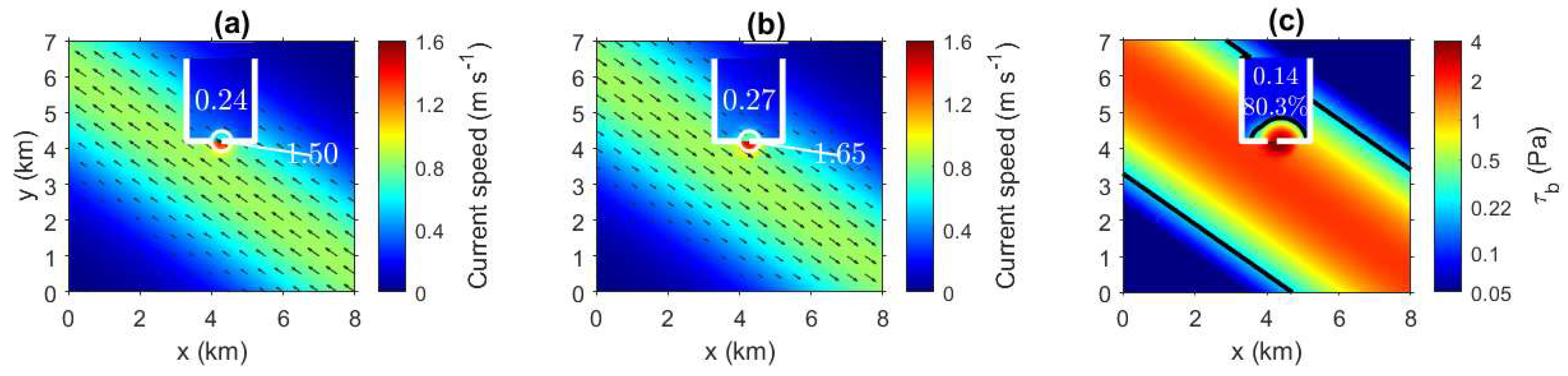
Key results are summarized in Table 4 (main text). Under Plan D, depth-averaged harbor velocity during spring tides is reduced to 0.24 m s−1 (flood) and 0.27 m s−1 (ebb), representing decreases of 68.4% and 67.9% from Scenario ①, respectively—a stronger reduction than under Plan B (300 m), reflecting the additional energy attenuation from the narrower aperture. The eastern tip peak ebb velocity reaches 1.65 m s−1, exceeding the Plan A value (1.53 m s−1) by 7.8% and reflecting the enhanced flow constriction through the narrower opening. The spring-tide tidal-mean bed shear stress averaged over the harbor area is 0.14 Pa, with 80.3% of the harbor area falling below τ c e = 0.22 Pa—slightly higher than the 76.8% reported for Plan A, consistent with the further suppression of internal circulation. Spring-tide net sediment import is 10.2 × 10⁶ kg per cycle, and the corresponding spring–neap weighted mean is approximately 6.8 × 10⁶ kg per cycle. The daily water exchange rate is 61.2%/day.
The step marginal efficiency ratio for the B → D transition (300 → 250 m) is 1.03, compared with 1.23 for the A → B transition (400 → 300 m) and 1.01 for the D → C transition (250 → 200 m). The monotonic decline of these ratios (1.23 → 1.03 → 1.01) confirms that the sedimentation–exchange trade-off deteriorates sharply between 250 and 300 m, localizing the onset of hydraulic choking to this 50 m interval and narrowing the previously identified 200–300 m transition range by half. The depth-averaged velocity field during peak flood and peak ebb, together with the tidal-mean bed shear stress distribution under Plan D, are shown in Figure A1.
Figure A1. Plan D (250 m entrance) hydrodynamic and bed shear stress fields. (a) Depth-averaged velocity at peak flood. (b) Depth-averaged velocity at peak ebb. (c) Spring-tide tidal-mean bed shear stress distribution. Note: In (a) and (b), color fill: current speed (m s−1); vectors: current direction; white solid lines: breakwaters. In (c), color scale is logarithmic (Pa); black contour: τ c e   = 0.22 Pa; white solid lines: breakwaters.
Jmse 14 01018 g0a1

References

  1. Huang, Z.; Xu, H.; Bai, Y.; Shi, F.; Wen, Z. Coastline changes and tidal current responses due to the large-scale reclamations in the Bohai Bay. J. Oceanol. Limnol. 2023, 41, 2045–2059. [Google Scholar] [CrossRef]
  2. Zhang, H.X.; Shen, Y.M.; Tang, J. Numerical investigation of successive land reclamation effects on hydrodynamics and water quality in Bohai Bay. Ocean Eng. 2023, 268, 113483. [Google Scholar] [CrossRef]
  3. Liu, S.; Li, G.; Liu, S.; Xing, L.; Pan, Y.; Yu, D. Impacts of reclamation on hydrodynamic and suspended sediment transport in the Bohai Sea. J. Geophys. Res. Ocean. 2024, 129, e2023JC020570. [Google Scholar] [CrossRef]
  4. Wu, Z.; Zhou, C.; Wang, P.; Fei, Z. Responses of tidal dynamic and water exchange capacity to coastline change in the Bohai Sea, China. Front. Mar. Sci. 2023, 10, 1118795. [Google Scholar] [CrossRef]
  5. Sun, J.; Zhang, M.; Zhou, J. Tidal responses of the semi-enclosed Bohai Sea to the long-term expansion of the Yellow River Delta. Front. Mar. Sci. 2025, 12, 1644888. [Google Scholar] [CrossRef]
  6. Zhu, L.; Hu, R.; Zhu, H.; Jiang, S.; Xu, Y.; Wang, N. Modeling studies of tidal dynamics and the associated responses to coastline changes in the Bohai Sea, China. Ocean Dyn. 2018, 68, 1625–1648. [Google Scholar] [CrossRef]
  7. Zhang, B.; Xiang, X.; Chen, Z.; Zhang, X.; Guo, J. Assessment of land reclamation effects on material transport in the Bohai Bay based on information entropy theory. Estuar. Coast. Shelf Sci. 2025, 326, 109544. [Google Scholar] [CrossRef]
  8. Chu, H.; Feng, Y.; Bai, D.; Wu, S.; Yuan, J.; Li, J.; Feng, B.; Jiang, W. Study on the geomorphological changes of deep troughs under the influence of reclamation in the Caofeidian. Estuar. Coast. Shelf Sci. 2024, 298, 108624. [Google Scholar] [CrossRef]
  9. Liang, H.; Kuang, C.; Olabarrieta, M.; Song, H.; Ma, Y.; Dong, Z.; Han, X.; Zuo, L.; Liu, Y. Morphodynamic responses of Caofeidian channel-shoal system to sequential large-scale land reclamation. Cont. Shelf Res. 2018, 165, 12–25. [Google Scholar] [CrossRef]
  10. Lu, Y.; Ji, R.; Zuo, L. Morphodynamic responses to the deep water harbor development in the Caofeidian sea area, China’s Bohai Bay. Coast. Eng. 2009, 56, 831–843. [Google Scholar] [CrossRef]
  11. Tseng, I.; Hsu, C.; Yeh, P.; Lin, T. Physical mechanism for seabed scouring around a breakwater—A case study in Mailiao Port. J. Mar. Sci. Eng. 2022, 10, 1386. [Google Scholar] [CrossRef]
  12. Yeganeh-Bakhtiary, A.; Houshangi, H.; Abolfathi, S. Lagrangian two-phase flow modeling of scour in front of vertical breakwater. Coast. Eng. J. 2020, 62, 252–266. [Google Scholar] [CrossRef]
  13. Xiao, Z.; Li, Z.; Zhang, J.; Zhang, W.; Yuan, M. Hydrodynamic analysis of a novel prefabricated permeable eco-friendly wharf with multi-compartment suction buckets and perforated circular caissons serving as breakwater. Ocean Eng. 2025, 341, 122549. [Google Scholar] [CrossRef]
  14. Romdani, A.; Chen, J.L.; Chien, H.; Lin, J.H.; Hung, C.K.; Huang, Y.Q. Downdrift port siltation adjacent to a river mouth: Mechanisms and effects of littoral sediment transport to the navigation channel. J. Waterw. Port Coast. Ocean Eng. 2022, 148, 05022001. [Google Scholar] [CrossRef]
  15. Elnabwy, M.T.; Elbeltagi, E.; El Banna, M.M.; Alshahri, A.H.; Kaloop, M.R. Harbor sedimentation management using numerical modeling and exploratory data analysis. Adv. Civ. Eng. 2024, 2024, 1209460. [Google Scholar] [CrossRef]
  16. Zhou, Z.; Ge, J.; Van Maren, D.S.; Wang, Z.B.; Kuai, Y.; Ding, P. Study of sediment transport in a tidal channel-shoal system: Lateral effects and slack-water dynamics. J. Geophys. Res. Ocean. 2021, 126, e2020JC016334. [Google Scholar] [CrossRef]
  17. Zhou, Z.; Stacey, M.T. Residual sediment transport in tidally energetic estuarine channels with lateral bathymetric variation. J. Geophys. Res. Ocean. 2020, 125, e2020JC016140. [Google Scholar] [CrossRef]
  18. Kim, S.I.; Seo, J.Y.; Park, J.-H.; Kim, P.J.; Kim, I.G.; Kim, K.M.; Ha, H.K. Imbalance of sediment transport in a meso-tidal bay: Effect of tidal pumping and residual circulation. Front. Mar. Sci. 2024, 11, 1362583. [Google Scholar] [CrossRef]
  19. Sharaan, M.; Lebleb, A.A.; ElZahar, M.M.H.; Iskander, M. Studying the tidal-induced water circulation pattern within EL-Burullus fishing harbor, Egypt, using CMS-PTM numerical modeling. Mar. Environ. Res. 2022, 180, 105726. [Google Scholar] [CrossRef]
  20. Alkhalidi, M.; Alsulaili, A. Enhancing marina sustainability: Water quality and flushing efficiency in marinas. J. Mar. Sci. Eng. 2024, 12, 649. [Google Scholar] [CrossRef]
  21. Yao, P.; Su, M.; Wang, Z.; van Rijn, L.C.; Stive, M.J.F.; Xu, C.; Chen, Y. Erosion behavior of sand–silt mixtures: Revisiting the erosion threshold. Water Resour. Res. 2022, 58, e2021WR031788. [Google Scholar] [CrossRef]
  22. Chen, D.; Zheng, J.; Zhang, C.; Guan, D.; Li, Y.; Huang, H. Threshold of surface erosion of cohesive sediments. Front. Mar. Sci. 2022, 9, 847985. [Google Scholar] [CrossRef]
  23. Chen, D.; Wang, Y.; Melville, B.; Huang, H.; Zhang, W. Critical shear stress for erosion of sand-mud mixtures and pure mud. Front. Mar. Sci. 2021, 8, 713039. [Google Scholar] [CrossRef]
  24. Dong, J.; Shi, J.; Zhao, J.; Zhang, C.; Xu, H. Wave energy assessment in the Bohai Sea and the Yellow Sea based on a 40-year hindcast. Water 2020, 12, 2087. [Google Scholar] [CrossRef]
  25. Zhou, Z.; Bian, C.; Wang, C.; Jiang, W.; Bi, R. Quantitative assessment on multiple timescale features and dynamics of sea surface suspended sediment concentration using remote sensing data. J. Geophys. Res. Ocean. 2017, 122, 8739–8752. [Google Scholar] [CrossRef]
  26. Lesser, G.R.; Roelvink, J.A.; van Kester, J.A.T.M.; Stelling, G.S. Development and validation of a three-dimensional morphological model. Coast. Eng. 2004, 51, 883–915. [Google Scholar] [CrossRef]
  27. Launder, B.E.; Spalding, D.B. The numerical computation of turbulent flows. In Numerical Prediction of Flow, Heat Transfer, Turbulence and Combustion; Pergamon: Oxford, UK, 1983; pp. 96–116. [Google Scholar] [CrossRef]
  28. Partheniades, E. Erosion and deposition of cohesive soils. J. Hydraul. Div. 1965, 91, 105–139. [Google Scholar] [CrossRef]
  29. Krone, R.B. Flume Studies of the Transport of Sediment in Estuarial Shoaling Processes: Final Report; Hydraulic Engineering Laboratory, University of California: Berkeley, CA, USA, 1962. [Google Scholar]
  30. Rijn, L.C. Sediment transport, part II: Suspended load transport. J. Hydraul. Eng. 1984, 110, 1613–1641. [Google Scholar] [CrossRef]
  31. van Rijn, L.C. Principles of Sediment Transport in Rivers, Estuaries and Coastal Seas; Aqua Publications: Amsterdam, The Netherlands, 1993. [Google Scholar]
  32. Egbert, G.D.; Erofeeva, S.Y. Efficient inverse modeling of barotropic ocean tides. J. Atmos. Ocean. Technol. 2002, 19, 183–204. [Google Scholar] [CrossRef]
  33. Ramakrishnan, B.; Gavali, M.; Jeyaraj, S. Comprehensive analysis of siltation behavior in the navigation channel of Deendayal Port (India): Field observations, numerical modeling, and engineering solutions. J. Coast. Res. 2024, 40, 138–149. [Google Scholar] [CrossRef]
  34. McCarroll, R.J.; Masselink, G.; Valiente, N.G.; Wiggins, M.; Scott, T.; Conley, D.C.; King, E.V. Impact of a headland-associated sandbank on shoreline dynamics. Geomorphology 2020, 355, 107065. [Google Scholar] [CrossRef]
  35. Jenkins, R.L.; Passeri, D.L.; Smith, C.G.; Thompson, D.M.; Smith, K.E.L. Modeling the effects of interior headland restoration on estuarine sediment transport processes in a marine-dominant estuary. Front. Mar. Sci. 2023, 10, 1217830. [Google Scholar] [CrossRef]
  36. Wu, T.; Qin, J. Influence of flow and sediment transport processes on sedimentation in groyne fields. J. Coast. Res. 2020, 95, 304–308. [Google Scholar] [CrossRef]
  37. Chang, J.; Lee, G.-H.; Ajama, O.D.; Li, W. Estimation of bed shear stress and settling velocity with inertial dissipation method of suspended sediment concentration in cohesive sediment environments. Front. Mar. Sci. 2024, 11, 1475565. [Google Scholar] [CrossRef]
  38. Savvidis, Y.; Keramaris, E. Study of water renewal and sedimentation of a square harbor encapsulated in a coastal front with seawalls due to wind-induced hydrodynamic circulation. Int. J. Sediment Res. 2021, 36, 373–383. [Google Scholar] [CrossRef]
  39. Hanegan, K.C.; FitzGerald, D.M.; Georgiou, I.Y.; Hughes, Z.J. Long-term sea level rise modeling of a basin-tidal inlet system reveals sediment sinks. Nat. Commun. 2023, 14, 7117. [Google Scholar] [CrossRef] [PubMed]
  40. Yang, Q.; Hu, S.; Fu, L.; Zhang, P.; Chu, N.; Liu, F.; Cai, H. Responses of tidal duration asymmetry to morphological changes in Lingding Bay of the Pearl River Estuary. Front. Mar. Sci. 2022, 9, 983182. [Google Scholar] [CrossRef]
  41. Romdani, A.; Chen, J.L.; Chien, H.; Lin, J.H.; Liao, C.Y.; Hou, C.C. Downdrift port siltation adjacent to a river mouth: Effects of mesotidal conditions and typhoon. J. Waterw. Port Coast. Ocean Eng. 2023, 149, 05022007. [Google Scholar] [CrossRef]
  42. Yuan, X.; Feng, X.; Hu, R.; Jiang, S.; Zhong, W. Study on the sediment transport flux and mechanism in the Bohai Strait at the tidal and monthly scales in summer. J. Ocean Univ. China 2023, 22, 75–87. [Google Scholar] [CrossRef]
  43. Shi, P.; Yang, W.; Xu, X.; Zhang, F. Response of hydrodynamic environment to land reclamation in Sanmen Bay, China over the last half-century. Front. Mar. Sci. 2024, 11, 1448565. [Google Scholar] [CrossRef]
  44. Lojek, O.; Goseberg, N.; Schlurmann, T. Projecting hydro-morphodynamic impacts of planned layout changes for a coastal harbor. J. Waterw. Port Coast. Ocean Eng. 2021, 147, 05021013. [Google Scholar] [CrossRef]
  45. Deng, X.; Wang, Z.; Ma, X. Impact of silted coastal port engineering construction on marine dynamic environment: A case study of Binhai Port. J. Mar. Sci. Eng. 2025, 13, 494. [Google Scholar] [CrossRef]
  46. Wang, J.; Chu, A.; Dai, Z.; Nienhuis, J. Delft3D model-based estuarine suspended sediment budget with morphodynamic changes of the channel-shoal complex in a mega fluvial-tidal delta. Eng. Appl. Comput. Fluid Mech. 2024, 18, 2300763. [Google Scholar] [CrossRef]
  47. Xu, T.; You, X. Numerical simulation of suspended sediment concentration by 3D coupled wave-current model in the Oujiang River Estuary, China. Cont. Shelf Res. 2017, 137, 13–24. [Google Scholar] [CrossRef]
Figure 1. Study area and computational grid. (a) Geographic setting. (b) Computational grid. Note: Near-field resolution 20–50 m; far-field 200–500 m. Triangles: tidal elevation stations T1–T4; circles: current speed stations C1–C3; squares: SSC stations S1–S2; red line: open boundary.
Jmse 14 01018 g001
Figure 2. Model validation results. (a) T1. (b) T2. (c) T4. (d) C1. (e) C2. (f) C3. (g) S1. (h) S2. Note: Black: observed; red: simulated. RMSE and NSE are annotated in panels (af) and mean relative bias is annotated in panels (g,h). Systematic underestimation during high-velocity periods in (g,h) reflects the absence of wave-enhanced bed shear stress in the model.
Jmse 14 01018 g002
Figure 3. Depth-averaged velocity fields during peak flood and peak ebb. (a) Scenario 1—no breakwater, peak flood. (b) Scenario 1—no breakwater, peak ebb. (c) Scenario 2—400 m entrance, peak flood. (d) Scenario 2—400 m entrance, peak ebb. Note: Color fill: current speed (m s−1; scale 0–1.6 m s−1); vectors: current direction; white solid lines: breakwaters; outer dashed box: headland jet acceleration zone; inner dashed box: harbor basin velocity gradient zone.
Jmse 14 01018 g003
Figure 4. Vorticity structure at the eastern breakwater head during peak ebb. (a) Surface vorticity (σ = 0.1)—peak ebb. (b) Vertical cross-section along the east breakwater axis. Note: Positive values (warm colors): counterclockwise rotation; negative values (cool colors): clockwise rotation. White contour: |ω| = 0.01 s−1. Dashed lines in (b): σ = 0.1 and σ = 0.9 reference levels.
Jmse 14 01018 g004
Figure 5. Spring-tide tidal-mean bed shear stress distribution. (a) Scenario 1—no breakwater. (b) Scenario 2—400 m entrance. Note: Color scale is logarithmic (Pa). Black contour in (a): τ c e = 0.22 Pa. White solid lines: breakwaters; white dashed ellipse: eastern tip peak stress zone.
Jmse 14 01018 g005
Figure 6. Spring-tide SSC distribution and net sediment flux under Scenario ②. (a) SSC vertical cross-section along harbor centerline. (b) Net sediment flux through harbor entrance (spring tide, Scenario 2). Note: In (a), late-ebb bottom resuspension pulse (~0.12 kg m−3) labeled. In (b), positive: into harbor; negative: outward; gray shading: flood-dominated high-concentration input period; net flux values for spring (14.8 × 10⁶ kg/cycle) and neap (4.9 × 10⁶ kg/cycle) are annotated.
Jmse 14 01018 g006
Figure 7. Reynolds flux decomposition at the harbor entrance under Scenario ② during spring tide (Days 21–22). (a) Lateral distribution of tidally integrated net sediment flux per unit width across the 400 m entrance. (b) Stacked contributions of advective (Fadv) and tidal pumping (Fpump) components for the eastern vortex sector and central + western sector. Note: In (a), horizontal axis: distance from the eastern breakwater head (0–400 m); vertical axis: net sediment flux per unit width (kg m−1 cycle−1); vertical dashed line at 150 m marks the vortex sector boundary; shaded area under the curve decomposed into advective (blue) and tidal pumping (orange) components. In (b), stacked bars show absolute flux contributions (×106 kg cycle−1) for the eastern vortex sector (0–150 m, ~38% of entrance width) and central + western sector (150–400 m, ~62% of entrance width); percentages above bars indicate each sector’s share of total net import (39% vs. 61%); advective component labeled within bars (−0.1 and 0.0 × 10⁶ kg cycle−1, respectively). Unit-width flux ratio (vortex sector/central sector ≈ 1.7) is annotated.
Jmse 14 01018 g007
Table 1. Summary of model configuration and key parameter settings.
CategoryParameterValue/Setting
GridHorizontal resolution20–50 m (near field); 200–500 m (far field)
Vertical layers10 σ-layers; 3 layers concentrated near bed
Time step60 s
SimulationTotal duration30 days
Spin-up periodDays 1–15
Analysis periodDays 15–30
Initial conditionsWater level0.0 m (cold start)
Velocity0.0 m s−1 (cold start)
SSC0.0 kg m−3 (cold start; 15-day spin-up allows equilibration)
Hydrodynamic boundaryTidal forcingM2, S2, O1, K1 from TPXO 9.0 [32]
Temperature/salinityNot included (barotropic configuration)
Wave–current couplingNot included (see Section 4)
Sediment boundaryOffshore SSC (spring tide)0.088 kg m−3
Offshore SSC (neap tide)0.051 kg m−3
Bed sedimentSediment classSingle cohesive fraction (fine silt)
Median grain size d500.063 mm
Sediment parametersCritical erosion stress τ c e 0.22 Pa
Critical deposition stress τ_cd0.10 Pa
Effective settling velocity w_s0.3 mm s−1
TurbulenceClosure schemeStandard k–ε (c1ε = 1.44, c2ε = 1.92, σ_k = 1.0, σ_ε = 1.3)
Bed roughnessManning coefficient n0.018 m−1/3 s
Table 2. Summary of numerical simulation scenarios.
ScenarioBreakwaterEntrance Width (m)Analysis PeriodPrimary Purpose
AbsentDays 15–30Background baseline
② (Plan A)Present400Days 15–30Current configuration
③ (Plan B)Present300Days 15–30Width sensitivity
④ (Plan D)Present250Days 15–30Width sensitivity
⑤ (Plan C)Present200Days 15–30Width sensitivity
Note: Plan D (250 m, Scenario ④) was added during revision to refine the hydraulic transition interval initially identified between Plans B and C.
Table 3. Parameter sensitivity analysis of key sediment transport metrics (Scenario ②, spring tide).
ParameterBaselineRangeDepositional Area (%)Net Flux (×106 kg/Cycle)
τ c e 0.22 Pa±20%70.2–82.4±2% (indirect)
w_s0.30 mm s−1±20%±1.5 pp (indirect)9.1–10.7
n (Manning)0.018±10%73.1–80.29.4–10.5
RSS composite68–838.8–11.0
Note: Depositional area = fraction of harbor area with tidal-mean τ b < τ c e during spring tide. Net flux = spring–neap weighted-mean entrance sediment import. RSS = root-sum-square composite of independent perturbations. Wave-coupling correction assessed separately in Section 4.
Table 4. Key hydrodynamic and sediment transport metrics across entrance width scenarios during spring tide.
PlanOpening (m)Net Sediment Flux (×106 kg/cycle)Change vs. Plan A (%)Water Exchange Rate (%/day)Change vs. Plan A (%)
A (current)40014.883.7
B30011.7−21.069.4−17.1
D25010.2−31.161.2−26.9
C2008.6−41.952.1−37.7
Note: Marginal efficiency ratio (% flux reduction per % exchange loss) declines monotonically: 1.23 (A → B), 1.03 (B → D), 1.01 (D → C), confirming onset of hydraulic choking behavior between 250 and 300 m.
Disclaimer/Publisher’s Note: The statements, opinions and data contained in all publications are solely those of the individual author(s) and contributor(s) and not of MDPI and/or the editor(s). MDPI and/or the editor(s) disclaim responsibility for any injury to people or property resulting from any ideas, methods, instructions or products referred to in the content.