A Study on the MSC-BiLSTM Ship Track Prediction Model Incorporating an Adaptive Attention Mechanism

Abstract

Accurate ship trajectory prediction is vital for intelligent maritime traffic management, yet conventional hybrid models often fail to balance local feature extraction, long-term dependency capture, and flexible feature weighting when processing AIS data. This paper proposes an MSC-BiLSTM-ATTENTION model that integrates trajectory clustering and an adaptive attention mechanism into a unified framework. Its fundamental advance over existing incremental hybrid architectures is twofold. First, a K-means clustering step groups trajectories with similar motion patterns before model training, effectively reducing the impact of data heterogeneity on prediction accuracy. Second, the deep learning backbone synergizes multi-scale convolution (MSC)—which captures local features at multiple temporal granularities via parallel kernels—with a bidirectional LSTM (BiLSTM) for forward–backward dependency learning, and an adaptive self-attention mechanism that dynamically optimizes feature weights to amplify critical navigation information. Extensive experiments on AIS data from the Gulf of Mexico and the U.S. Atlantic Coast, covering four seasons, benchmark the model against attention-enhanced architectures including Transformer, CNN-BiLSTM-ATTENTION, and DenseNet-BiGRU-ATTENTION across two distinct regions. The proposed model achieves significant improvements in predicting longitude, latitude, speed over ground, and course over ground, reducing MAE by over 76.9% and RMSE by over 65.3% compared with the strongest baseline. Ablation studies confirm that the synergy of all three modules is essential. The results demonstrate the model’s effectiveness and its practical value for intelligent maritime supervision, navigation risk warning, and waterborne traffic management.

1. Introduction

As global economic integration advances, the shipping industry develops rapidly as the core carrier of international trade. Global port throughput rises year by year. Vessels exhibit clear trends toward larger size and higher intelligence. Projections indicate a 2–3% average annual growth in container trade volume from 2024 to 2030. Geopolitical factors and route adjustments cause a 6% increase in tonne-miles from detours in 2024 [1]. These factors lead to continuously rising maritime traffic density and increasingly complex navigation scenarios. Against this background, the shipping industry faces severe safety challenges. Accidents occur frequently in congested navigation areas such as coastal waters and narrow channels. Global maritime safety levels have generally improved. In congested navigation areas, this proportion can exceed 75% [2]. These accidents cause huge losses of life and property and damage marine ecosystems. They also seriously disrupt the stable operation of global shipping supply chains. Therefore, real-time awareness of vessel dynamics and accurate trajectory prediction constitute key measures. These measures enhance the intelligence level of maritime control. They also effectively prevent maritime accidents.

To address maritime vessel monitoring challenges, the International Maritime Organization (IMO) amended the SOLAS convention. The amendment mandates the installation of Automatic Identification Systems (AISs) on ocean-going vessels of 300 gross tonnage and above, near-shore vessels of 500 gross tonnage and above, and all passenger vessels. This regulation achieved full implementation by the end of 2004 [3,4]. An AIS relies on VHF technology. It broadcasts and receives vessel core parameters such as longitude, latitude, and speed over ground in real time. The update frequency ranges from 2 to 10 s per transmission [5]. This provides continuous and reliable data support for trajectory prediction. AIS data offers advantages over traditional radar monitoring and human visual observation. These include wide coverage, high accuracy, strong real-time performance, and rich dimensionality. These advantages make data-driven trajectory prediction a research hotspot in the maritime field.

Ship trajectory prediction methods fall into two main categories: traditional methods and deep learning methods [6]. These two categories differ significantly in applicable scenarios and prediction performance. Traditional methods include Kalman filters and particle filters [7]. These methods perform deduction based on fixed vessel kinematic models. They offer the advantages of mature theory and high computational efficiency. Under ideal conditions with accurate models and a Gaussian noise distribution, they provide stable short-term prediction performance. However, these model-driven approaches heavily rely on predefined motion assumptions, which limit their ability to adapt to complex and highly dynamic maritime environments. For example, Tong et al. [8] proposed a Kalman filtering strategy. This strategy filters vessel node position data to improve trajectory prediction accuracy in curved inland waterways. Wang et al. [9] proposed a Transformer-based trajectory prediction model (TPTrans) that combines convolutional layers with a Transformer encoder–decoder to capture both local spatiotemporal features and global dependencies. Qiang et al. [10] developed a Motion-Inspired Spatial–Temporal Transformer (MSTFormer) that integrates motion modeling with a Transformer network to enhance trajectory prediction accuracy. Fossen et al. [11] applied an extended Kalman filter to real-time AIS data. This application optimizes short-term prediction in dynamic sea areas. Zhang et al. [12] proposed a Gated Spatio-Temporal Graph Aggregation Network (G-STGAN) for ship trajectory prediction in dynamic traffic scenarios. However, these models rely on pre-defined and often simplified kinematic or dynamic models. They fail to adapt to dynamic changes caused by natural factors such as wind, waves, and ocean currents, as well as human factors such as vessel collision avoidance and route adjustments. Their prediction accuracy and generalization capability remain limited [13]. Therefore, they cannot meet the control requirements of complex maritime scenarios.

Temporal models such as LSTM are widely applied in ship trajectory prediction; however, the cited works differ in their focus: one approach extracts cross-variable correlations without inter-vessel interaction, while the other learns multi-vessel interaction graphs, though the latter depends on the quality of the initial distribution [14,15]. The CNN-MTABiGRU model captures temporal dependencies through a bidirectional GRU and temporal attention, but its evaluation on a single vessel in a single waterway limits its generalisability [16]. Yang et al. [17] improved short-term accuracy by combining data denoising with Bi-LSTM; however, their model considers only single-vessel motion and neglects environmental factors and multi-ship interactions, which reduces its reliability in complex maritime traffic. Jiang et al. [18] integrated Transformer with LSTM to capture long-range spatiotemporal dependencies, but their model fails to account for external factors such as weather conditions or multi-vessel encounters. Chen et al. [19] addressed insufficient local feature extraction and equal temporal weighting by introducing a trajectory direction vector (TDV) and an attention mechanism that adaptively emphasises course and speed variations; yet their method still relies solely on AIS data and does not incorporate radar or environmental information. Despite the gating mechanisms in LSTM and GRU networks that are designed to alleviate the vanishing gradient problem inherent in traditional RNNs, these networks still struggle to learn dependencies over extremely long sequences, which can lead to a decline in prediction accuracy for complex trajectory patterns [20].

Zhang et al. [21] proposed a memory-enhanced network with goal-driven decoding for long-term prediction; however, it still models only single-vessel trajectories and fails to account for multi-vessel interactions or environmental factors. While CNN–RNN hybrids are widely adopted for trajectory prediction, their designs differ notably in feature extraction and temporal modelling. Bi et al. [22] fuse AIS data with marine environmental variables via CNN-GRU and multi-head attention, yet this fusion introduces additional data complexity. Liu et al. [23] incorporate residual connections into a CNN-GRU-attention structure to improve feature reuse, but this improvement incurs increased computational cost. Lin et al. [24] replace the standard TCN with a tiered-TCN for multi-scale temporal capture, although their relatively deep network may cause a heavier parameter load. Zaman et al. [25] applied CNN and DNN to learn trajectory patterns from preprocessed AIS data; CNN achieved notably lower errors, but their models were tested on a small set of vessels and lacked attention mechanisms that adaptively weight input features.

Table 1. Summary of related methods and their limitations.

Method Category	Key References	Main Limitations	How the Proposed Model Differs
Traditional model-based	[7,8,9,10,11,12,13]	Rely on predefined kinematic assumptions; fail in complex dynamic environments	Fully data-driven; requires no motion model assumptions
Recurrent networks (LSTM/GRU/BiLSTM)	[14,15,16,17,18,19,20]	Lacks local feature extraction; struggles with very long sequences	MSC supplies multi-scale local features; BiLSTM retained for sequence modeling
CNN-RNN hybrids	[21,22,23,24,25]	Use single-scale convolutions; miss multi-granularity patterns	MSC captures features at multiple temporal scales via parallel kernels
Attention-enhanced models	[5,19,21]	Attention operates on single-scale features; few integrate clustering	Self-attention weights multi-scale features; K-means preprocessing included
Clustering and segmentation	[26,28,30,31]	Applied mainly for analysis, not for end-to-end prediction	K-means clustering embedded as a preprocessing step in the prediction pipeline

presents a systematic summary of the core methodologies, advantages, and limitations of representative studies across five method categories. Traditional model-based methods [7,8,9,10,11,12,13] depend on predefined kinematic assumptions that restrict adaptability in complex maritime environments. Recurrent architectures [14,15,16,17,18,19,20] capture temporal dependencies effectively but lack dedicated modules for local feature extraction. CNN-RNN hybrids [21,22,23,24,25] enhance local feature learning but employ predominantly single-scale convolutions and often overlook multi-granularity temporal patterns. Attention-enhanced models [5,19,21] weight features dynamically; however, they seldom integrate multi-scale extraction or trajectory clustering into a unified framework. Clustering-based methods [26,27,28,29] serve primarily traffic pattern analysis rather than end-to-end prediction. The proposed MSC-BiLSTM-ATTENTION model addresses these gaps through two integrated innovations. First, a K-means clustering step partitions trajectories into homogeneous groups before model training, which reduces the impact of data heterogeneity on prediction accuracy. Second, a synergistic architecture combines multi-scale convolution, bidirectional LSTM, and adaptive self-attention to jointly handle local feature extraction, long-term dependency capture, and dynamic feature weighting within a single framework.

In summary, existing trajectory prediction models suffer from insufficient feature extraction and inflexible weight allocation. To address these problems, this paper proposes an MSC-BiLSTM trajectory prediction method that integrates an adaptive attention mechanism. The method incorporates clustering characteristics of trajectory data and features of AIS data. First, we preprocess the raw AIS data by removing outliers and filling missing values. We then apply the K-means algorithm to cluster the data. This reduces the impact of data heterogeneity. Next, we construct a hybrid model. The model uses MSC to extract deep local features. It uses BiLSTM to capture temporal dependencies bidirectionally. It also introduces an adaptive attention mechanism to dynamically allocate weights. This strengthens key features. The method provides a high-accuracy, highly adaptable solution for ship trajectory prediction. The contributions of this paper are as follows:

(1)

Existing hybrid models frequently fail to integrate local feature extraction, bidirectional temporal modeling, and dynamic weight allocation within a single framework, which leads to inadequate capture of complex trajectory patterns. This paper addresses this limitation by proposing an MSC-BiLSTM model equipped with an adaptive attention mechanism that unifies these three capabilities.

(2)

The heterogeneity of AIS data across different vessels and navigation scenarios significantly degrades prediction accuracy in conventional approaches. This paper introduces a K-means clustering preprocessing strategy that groups trajectories with similar motion patterns before model training, which effectively reduces the adverse impact of data heterogeneity on prediction performance.

(3)

Many existing studies evaluate their models on limited datasets or against a narrow set of baselines, which makes performance claims difficult to generalise. This paper conducts multiple comparative experiments across four seasons and two distinct navigation regions (Gulf of Mexico open waters and Atlantic Coast confined waterways), benchmarking the proposed model against mainstream methods and systematically verifying its superiority and robustness across diverse maritime scenarios.

The remainder of this paper is organized as follows. Section 2 describes the data preprocessing, trajectory clustering, and the hybrid model architecture. Section 3 defines the evaluation metrics and presents the comparative experiments and ablation study results. Section 4 summarizes the findings, discusses limitations, and suggests future research directions. For the reader’s convenience, the abbreviations used throughout this paper are listed in

Table 2. List of abbreviations.

Abbreviation	Full Name
AIS	Automatic Identification System
BiGRU	Bidirectional Gated Recurrent Unit
BiLSTM	Bidirectional Long Short-Term Memory
CNN	Convolutional Neural Network
COG	Course Over Ground
GRU	Gated Recurrent Unit
K-Means	K-Means Clustering
LSTM	Long Short-Term Memory
MAE	Mean Absolute Error
MMSI	Maritime Mobile Service Identity
MSC	Multi-Scale Convolution
MSE	Mean Squared Error
RMSE	Root Mean Square Error
SOG	Speed Over Ground

.

2. A Ship Trajectory Prediction Framework and Method Integrating an Adaptive Attention Mechanism

2.1. Ship Trajectory Prediction Framework Integrating an Adaptive Attention Mechanism

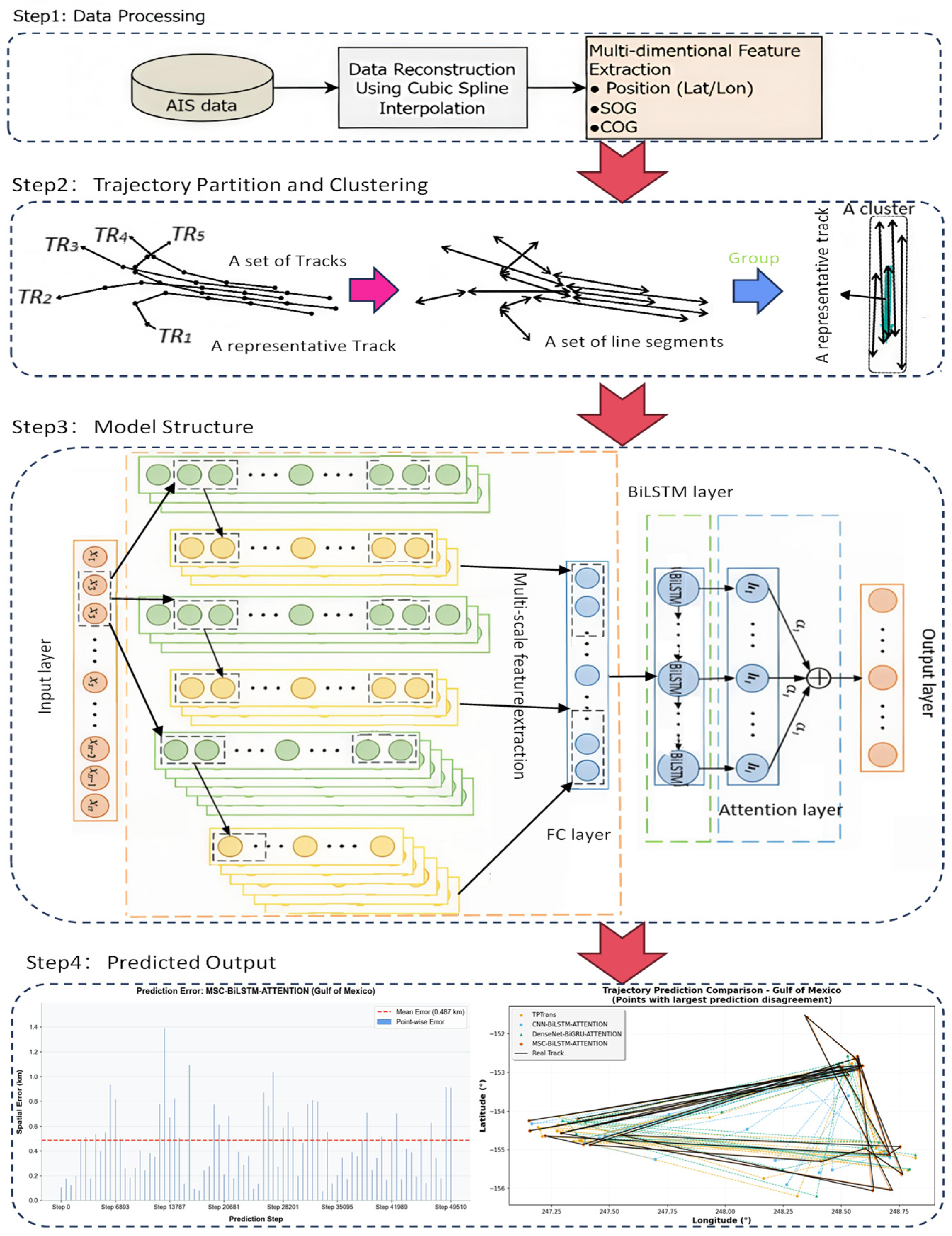
To achieve high-accuracy and strong-generalization ship trajectory prediction in complex maritime scenarios, this paper proposes an MSC-BiLSTM prediction model that integrates trajectory clustering and an adaptive attention mechanism. The model takes raw AIS data as input. It processes the data through four core modules: preprocessing, trajectory clustering, feature extraction, and prediction output. The model finally outputs the future longitude, latitude, course, and speed of the vessel. Figure 1 shows the overall framework of the model.

• AIS data preprocessing

The model acquires raw AIS data from public data sources. It filters and sorts the data by vessel MMSI and time period. It removes outliers such as abrupt position changes and speed limit violations. It then interpolates missing values. Finally, it applies min-max normalization to scale features including longitude, latitude, course, and speed over ground to the [0,1] interval. This provides high-quality data input for subsequent clustering and prediction.

• Trajectory segmentation and clustering

Based on the preprocessed AIS data, the model extracts feature points using rates of change in course and speed. It segments trajectories at these points. It measures similarity using a fused distance metric. It then clusters the trajectory segments using an improved K-means algorithm. The clustering groups trajectories with high similarity into the same cluster and maintains large differentiation between different clusters. This effectively reduces the impact of vessel navigation behavior heterogeneity on the prediction model.

• Multi-module feature extraction

The model feeds the trajectory sequences within each cluster into the hybrid model. First, it uses a multi-scale convolutional neural network (MSC) to extract deep local features such as sudden speed changes and course turns. It then feeds these local features into a bidirectional long short-term memory network (BiLSTM). The BiLSTM captures forward and backward temporal dependencies through its forward and reverse units, integrating contextual information. Finally, the model passes the BiLSTM-output temporal features into a self-attention mechanism. The self-attention mechanism dynamically computes weights for each feature, highlighting the key information that plays a critical role in trajectory prediction.

• Trajectory prediction and result analysis

The model feeds the feature vectors enhanced by the adaptive attention mechanism into a fully connected layer. This layer outputs the predicted future longitude, latitude, course, and speed over ground of the vessel. The paper conducts comparative experiments using real AIS data. It compares the proposed model with baseline models such as MSC and BiLSTM. It evaluates prediction performance using mean absolute error (MAE) and root mean square error (RMSE). These metrics validate the effectiveness and superiority of the proposed model. Finally, the paper analyzes the prediction results using trajectory fitting plots and error statistics tables.

2.2. Method

2.2.1. Ship Trajectory Segmentation and Clustering Method

(i)

Segmentation method

A vessel’s complete trajectory often contains multiple motion states, such as port entry/exit, cruising, and turning. If we directly use the entire trajectory as a sample, behavioral features from different stages interfere with each other. This makes it difficult to train an accurate prediction model. Moreover, trajectory segmentation increases the number of effective samples. It enables the model to learn richer local motion patterns. It also facilitates the subsequent clustering of sub-segments with similar navigation features into the same category, allowing cluster-specific modeling. Therefore, we need to segment the original long trajectory to extract sub-segments with consistent motion patterns.

Given that vessel navigation patterns in the two study areas exhibit distinct characteristics (open-sea traffic in the Gulf of Mexico versus confined port approaches on the Atlantic Coast), the feature-point segmentation method based on rates of change in course or speed fails to generate a sufficient number of effective sub-segments. In contrast, fixed-window sliding segmentation ensures uniform sub-segment length and sufficient sample size, which facilitates subsequent clustering and model training. Based on this consideration, this paper adopts the fixed-window sliding segmentation method.

Let the original trajectory sequence be $T=\{p_1, p_2,\dots , p_N\}$, where $p_t=[{\mathit{lon}}_t,{\mathit{lat}}_t,{\mathit{sog}}_t,{\mathit{cog}}_t]$. Here, ${\mathit{lon}}_t$ and ${\mathit{lat}}_t$ represent the vessel’s longitude and latitude at time t, respectively, while ${\mathit{sog}}_t$ and ${\mathit{cog}}_t$ denote the vessel’s speed over ground and course over ground at time t, respectively. The window length L = 60 min and step size S = 120 min were chosen to ensure each sub-segment captures a complete maneuvering cycle while maintaining sample diversity through partial overlap. Tests with alternative window lengths confirmed that this configuration provides the best trade-off between trajectory granularity and prediction accuracy. Following the sliding-window trajectory segmentation framework established in [26] for AIS data, the representation of each sub-segment is calculated by Equation (1):

$$s_k=\{p_{k\cdot S},p_{k\cdot S+1},\cdots ,p_{k\cdot S+L-1}\},k=0,1,\cdots ,\left[{\displaystyle \frac{N-L}{S}}\right]$$

(1)

where $\lfloor {\displaystyle \frac{N-L}{S}}\rfloor$ denotes the floor function, ensuring uniform sub-segment length and eliminating redundancy. The window length L = 60 (min) guarantees that each sub-segment contains sufficient vessel motion information. The step size S = 120 (min) introduces partial overlap between consecutive sub-segments, maintaining sample diversity while controlling the total number of sub-segments.

(ii)

Clustering method

After completing trajectory segmentation, each sub-segment exhibits relatively consistent motion states. However, significant navigation pattern differences may still exist among different sub-segments. If we treat all sub-segments as homogeneous samples and input them into a single prediction model, features from different patterns interfere with each other. This limits the model’s fitting ability and generalization performance. It should be noted that such pattern differences arise not only from operational decisions but also from the environmental conditions under which vessels navigate—for instance, the presence of sea ice fundamentally alters vessel dynamics through complex ice–structure–water interactions [30]. Therefore, we need to cluster the sub-segments. We group sub-segments with similar navigation features into the same cluster. Subsequently, we either build separate models for different clusters or use unified parameters within each cluster. This reduces the impact of data heterogeneity on prediction accuracy.

To effectively identify different navigation patterns, this paper adopts a “feature extraction–feature fusion–K-Means clustering” strategy. The rationale for this strategy is as follows. A single type of feature (e.g., only temporal features) cannot fully characterize navigation patterns. Fusing temporal features (such as speed and course) with statistical features (such as mean and standard deviation of course) provides a more complete representation of the motion law of each sub-segment. Standardizing both types of features before fusion eliminates dimensional differences and preserves multi-dimensional information. The K-Means algorithm offers high computational efficiency and ease of implementation, making it suitable for the tens of thousands of sub-segments in this study. In summary, this paper adopts this feature-fusion clustering method. The specific steps are as follows:

• Temporal feature extraction

Each sub-segment contains four basic motion parameters: longitude, latitude, speed over ground, and course over ground. To preserve the complete temporal information of each sub-segment, all sub-segments are first resampled to a fixed length M = 50 (points) and then flattened into a one-dimensional vector. The temporal feature extraction follows the multi-dimensional trajectory parameter flattening approach proposed in [27], as expressed by Equation (2):

$$f_{ts}=[p_1,p_2,\dots ,p_M]\in R^{4M}$$

(2)

Since the 4M-dimensional feature vector has excessively high dimensionality, Principal Component Analysis (PCA) is applied to reduce it, following the PCA-based trajectory feature decomposition method established in [31]. The reduced dimension was set to 20, which retained 99.16% of the total variance in the flattened temporal features, ensuring minimal information loss while significantly reducing computational complexity. The resulting 20-dimensional temporal feature vector is calculated by Equation (3). In Equations (2) and (3), $M=50$ denotes the fixed number of resampled points per sub-segment, $f_{\mathrm{temp}}\in R^{4M}$ is the flattened one-dimensional feature vector, and $f_{\mathrm{pca}}\in R^{20}$ is the reduced 20-dimensional feature vector obtained by PCA.

$$f_{ts}^{pca}=\mathrm{PCA}(f_{ts})\in R^{20}$$

(3)

2.

Statistical feature extraction

At the same time, the model extracts global statistical features from each sub-segment to fully capture its overall motion characteristics. These features include: the longitude and latitude of the start and end points; the mean and standard deviation of longitude, latitude, speed, and course; the cumulative changes in course and speed; the sub-segment length; and the duration. These features together form a 22-dimensional statistical feature vector $f_{\mathit{stat}}\in R^{22}$.

3.

Feature fusion and clustering

The concatenation of heterogeneous trajectory features follows the multi-feature fusion paradigm for ship trajectory data processing [28]. The reduced-dimensional temporal features and the statistical features are concatenated to obtain a 42-dimensional fused feature vector, as expressed by Equation (4):

$$f_{fusion}=[f^{pca},f_{stat}]\in R^{42}$$

(4)

After standardizing the fused feature vectors to eliminate dimensional effects, the K-Means algorithm is applied for clustering. The K-Means objective function that minimises the within-cluster sum of squares follows the trajectory clustering method in [29], as expressed by Equation (5):

$$min{{\displaystyle \sum _{i=1}^K{\displaystyle \sum _{x\in C_i}‖x-{\mu }_i‖}}}^2$$

(5)

The number of clusters K = 3 was determined through the elbow method and validated by clustering quality metrics; a detailed quantitative evaluation is presented in Section 3.2. where ${\mu }_i$ denotes the centroid of the i-th cluster, $C_i$ represents the set of sub-segments belonging to the i-th cluster, and $\parallel x-{\mu }_i{\parallel }^2$ is the squared Euclidean distance between the sub-segment feature vector x and the centroid ${\mu }_i$.

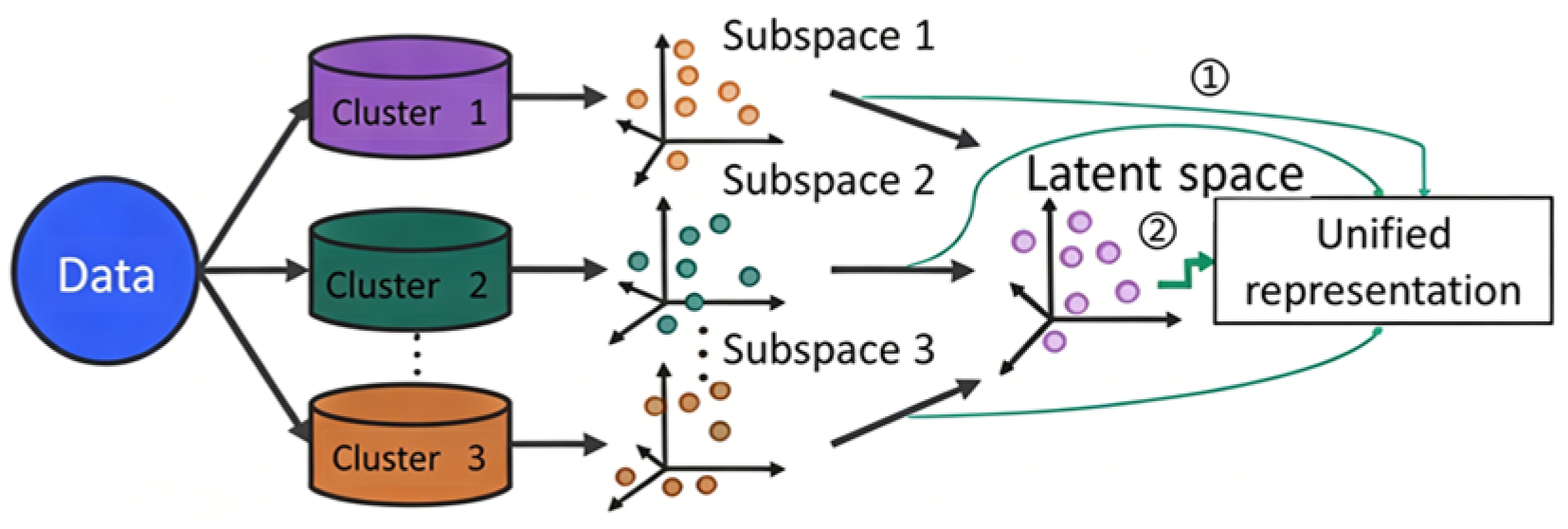
Figure 2 illustrates the feature fusion clustering process. This method first clusters the raw data into multiple clusters. It then constructs a dedicated feature subspace for each cluster to extract local features. Next, it maps the multi-subspace features to a shared latent space. Finally, it fuses them to generate a global unified feature representation. This achieves effective integration of local and global features.

2.2.2. MSC-BiLSTM Ship Trajectory Prediction Model Integrating an Adaptive Attention Mechanism

(i)

Multi-scale feature extraction model

Multi-scale convolution (MSC) is an important extension of CNN. MSC is specifically designed for one-dimensional time-series data. Its core advantage lies in using multiple parallel convolutional kernels of different scales. These kernels extract multi-level local features from time-series sequences. MSC balances local details with a global receptive field. This enhances the model’s ability to capture features across different time spans, such as sudden speed changes and course turns [32]. At the same time, weight sharing controls the parameter size. This makes MSC suitable for mining features from one-dimensional time-series data like AIS trajectories. Researchers have widely applied MSC in time-series signal analysis and prediction [33].

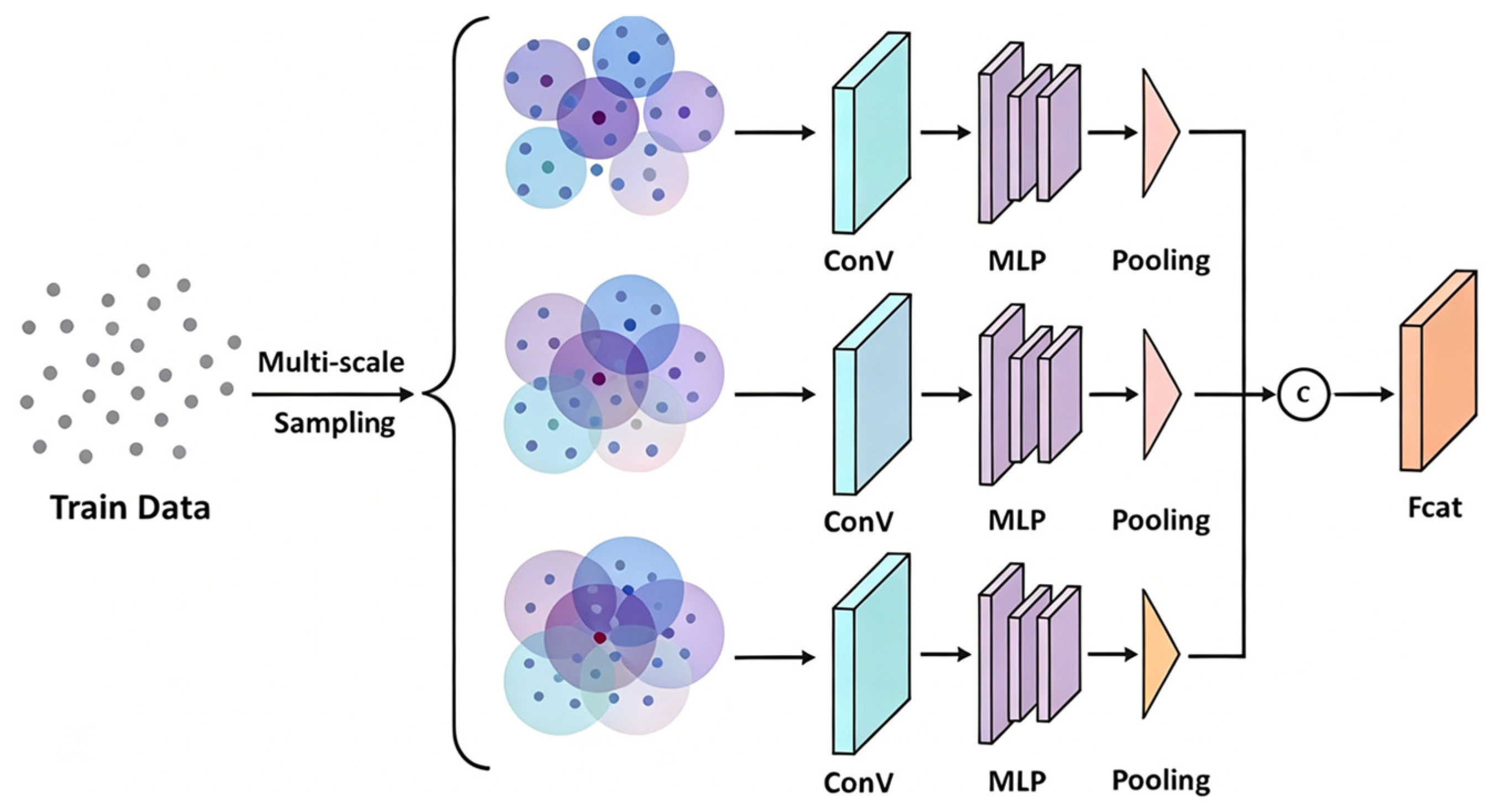
Figure 3 illustrates the core architecture of MSC. The architecture includes an input layer, a multi-scale convolutional layer, a pooling layer, and a fully connected layer. The input layer receives the preprocessed AIS time-series tensor. The multi-scale convolutional layer employs multiple one-dimensional convolutional kernels of different sizes. These kernels perform parallel sliding operations. They capture local features of AIS data at different temporal granularities. The outputs of all convolutional kernels concatenate along the channel dimension. This forms a rich multi-scale feature sequence [34]. The mathematical expression for a single-scale convolution can be expressed by Equation (6).

$$y_i^{\left(s\right)}=\sigma \left({\displaystyle \sum _{k=0}^{K_s-1}{w}_k^{\left(s\right)}\cdot x_{i+k}+b^{\left(s\right)}}\right)$$

(6)

where $K_s$ denotes the length of the $s$-th convolutional kernel ($s=1,2,3$ corresponding to the three parallel branches), $w_k^{\left(s\right)}$ represents the corresponding weight, $b^{\left(s\right)}$ is the bias term, and $\sigma$ denotes the ReLU activation function.

After concatenation, the outputs from different scales enter the pooling layer. The pooling layer downsamples the multi-scale feature sequence, typically using max pooling. It preserves the key peak features at each scale. This reduces parameters and mitigates overfitting. The fully connected layer maps the high-dimensional features to a one-dimensional vector. It integrates multi-scale local features into global features. This provides a suitable input for integration with the BiLSTM layer and the attention mechanism. Compared with single-scale CNNs and traditional temporal models, MSC directly processes one-dimensional AIS time-series data. It achieves high training efficiency. It simultaneously captures short-term abrupt changes and long-term trends [35]. In the hybrid model of this paper, MSC serves as the multi-scale local feature extraction module. It lays a richer foundation for subsequent temporal dependency capture and key feature enhancement.

To fully mine diversified spatial and temporal characteristics of vessel AIS trajectories, convolution operations with diverse receptive fields are deployed in the feature extraction stage. Such a multi-kernel design enables the model to perceive feature differences at different perception ranges, thereby enhancing the comprehensive feature extraction capability for complex and changeable navigation motion patterns.

(ii)

BiLSTM model

Long Short-Term Memory (LSTM) is a recurrent neural network variant. It solves the long-term dependency problem of traditional RNNs. LSTM introduces a gating mechanism (forget gate, input gate, output gate) and a cell state. It effectively mitigates the vanishing and exploding gradient problems. Compared with GRU, LSTM has stronger memory and expression capabilities. It controls information flow more precisely. LSTM is suitable for modeling complex time-series data.

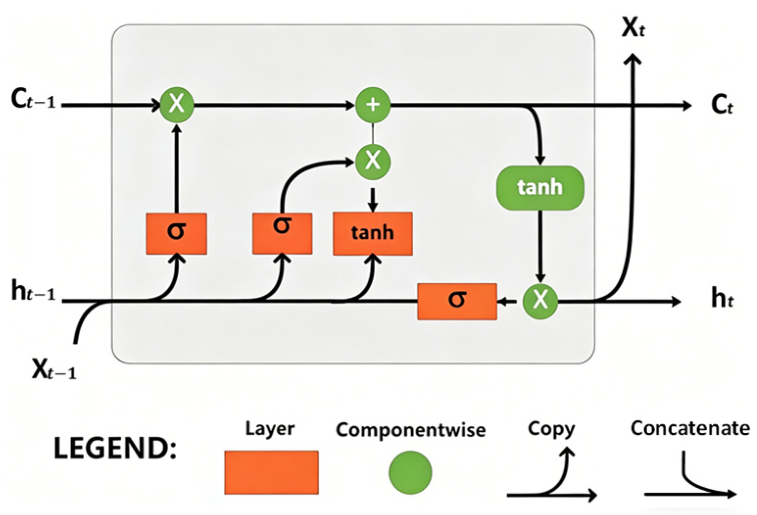
Figure 4 shows the core structure of LSTM. BiLSTM consists of two LSTM layers with opposite directions. It controls information transmission through the forget gate, input gate, and output gate [36]. The core formulas of the LSTM unit are as follows:

$$f_t=\sigma (W_f\cdot [h_{t-1},x_t]+b_f)$$

(7)

$$i_t=\sigma (W_i\cdot [h_{t-1},x_t]+b_i)$$

(8)

$${\tilde{C}}_t=tanh(W_C\cdot [h_{t-1},x_t]+b_C)$$

(9)

$$C_t=f_t\odot C_{t-1}+i_t\odot {\tilde{C}}_t$$

(10)

$$o_t=\sigma (W_o\cdot [h_{t-1},x_t]+b_o)$$

(11)

$$h_t=o_t\odot tanh(C_t)$$

(12)

In Equations (7)–(12), $f_t$, $i_t$, and $o_t$ denote the forget gate, input gate, and output gate activations at time step $t$, respectively; $C_t$ represents the cell state, and $h_t$ represents the hidden state. $x_t$ is the input vector at time $t$, and $h_{t-1}$ is the hidden state from the previous time step. $\sigma$ denotes the sigmoid activation function and $\odot$ denotes element-wise (Hadamard) multiplication. $W_f,W_i,W_c,W_o$ and $U_f,U_i,U_c,U_o$ are the weight matrices for the input $x_t$ and the recurrent hidden state $h_{t-1}$, respectively, and $b_f,b_i,b_c,b_o$ are the corresponding bias vectors.

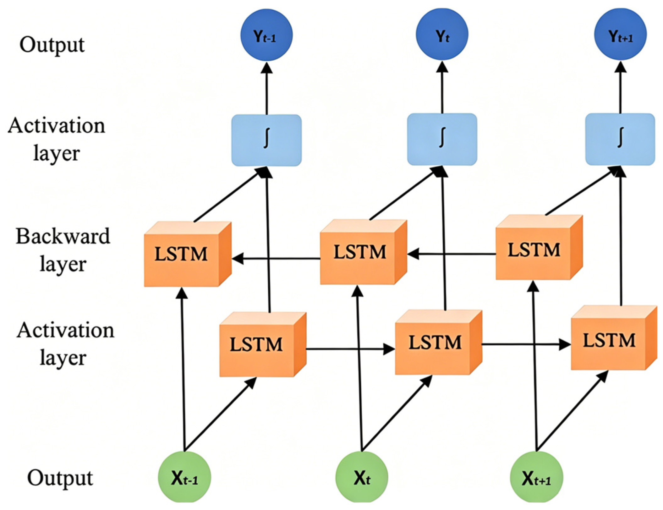
Figure 5 presents a schematic diagram of the BiLSTM. The forward LSTM captures forward dependencies in the AIS data from the beginning of the time series, such as continuous changes in speed and course. The backward LSTM captures backward dependencies from the end of the time series, such as the influence of future trajectory segments on the current state. The hidden layer outputs of the two LSTMs are concatenated with weights to form the final BiLSTM feature vector. The relevant definitions and formulas for the BiLSTM network are as follows:

$${\overrightarrow{h}}_t=\mathrm{LSTM}(x_t,{\overrightarrow{h}}_{t-1})$$

(13)

$$\overleftarrow{h_t}=\mathrm{LSTM}(x_t,{\overleftarrow{h}}_{t-1})$$

(14)

$$h_t=w_t\overrightarrow{h_t}+v_t\overleftarrow{h_t}+b_t$$

(15)

In Equations (13)–(15), ${\mathbf{x}}_t$ denotes the input at time step $t$; ${\overrightarrow{h}}_{t-1}$ and ${\overleftarrow{h}}_{t-1}$ represent the forward and backward hidden states from the previous time step, respectively; $\mathrm{L}\mathrm{S}\mathrm{T}\mathrm{M}(\cdot )$ denotes the nonlinear transformation performed by the LSTM cell. $w_t$ and $v_t$ are the weight matrices applied to the forward and backward hidden states, respectively, and $b_t$ is the bias term. The final BiLSTM output is obtained by concatenating the forward and backward hidden states.

Ship trajectory prediction often depends on both historical sequences and future states. A unidirectional LSTM relies only on past information and thus cannot fully model this bidirectional dependency. BiLSTM effectively solves this problem through bidirectional temporal modeling [37]. In the hybrid model of this paper, BiLSTM receives local features extracted by the multi-scale convolution (MSC). It bidirectionally captures the temporal dependencies in trajectory data. It integrates local features with contextual information. This provides high-quality temporal feature support for the subsequent adaptive attention mechanism, further improving trajectory prediction accuracy [38]. Compared with unidirectional LSTM, BiLSTM more completely mines the bidirectional temporal dependencies in trajectory data. Its parameter count increases slightly, but its prediction accuracy improves significantly.

To fully explore the complex time-series correlation of sailing movement, a bidirectional learning framework is adopted in this study. It can deeply mine the inherent connection between continuous navigation frames, overcoming the defect of single-path feature learning in conventional recurrent networks.

(iii)

Self-attention mechanism

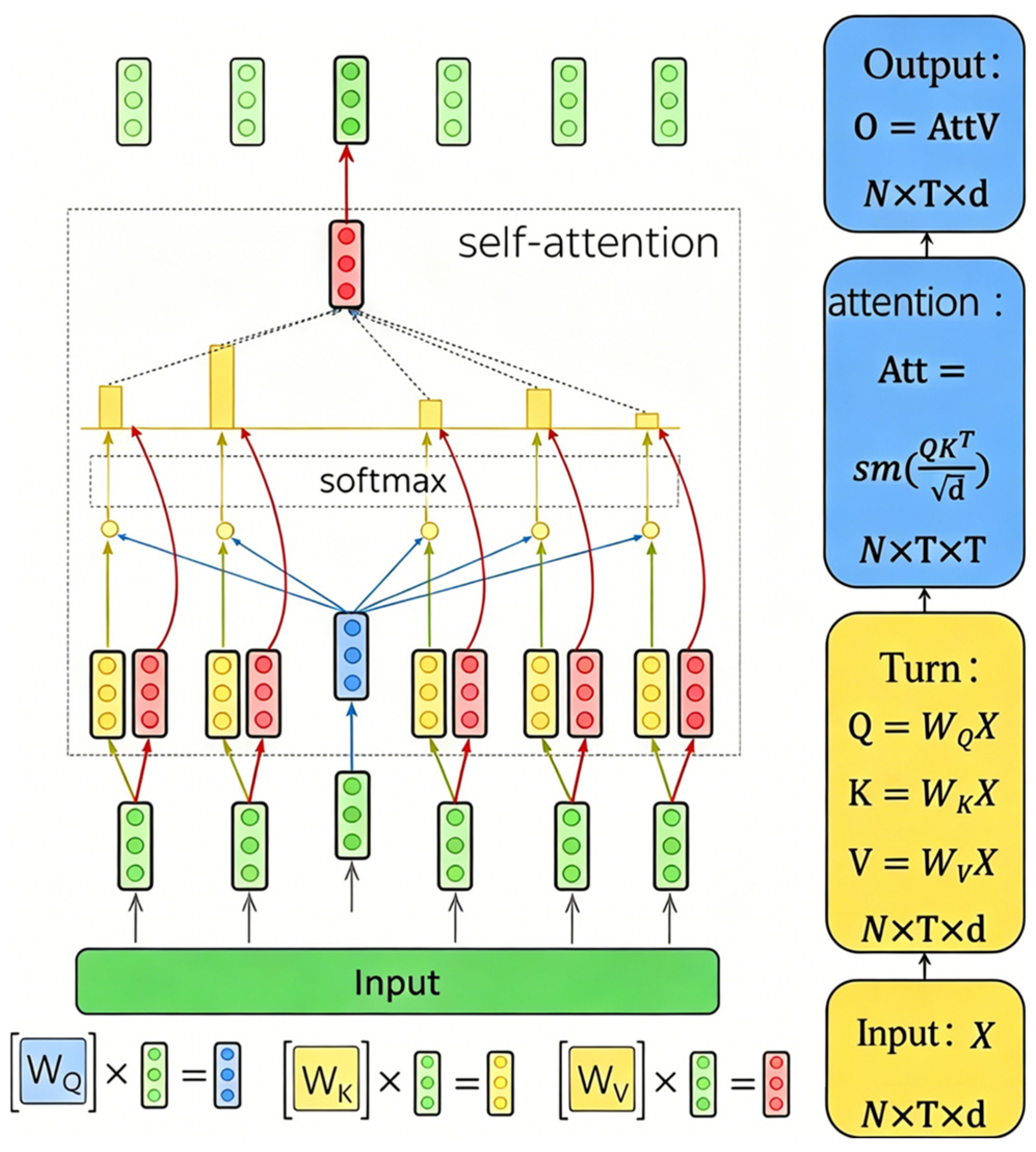
Figure 6 illustrates the self-attention mechanism. Self-attention is a feature enhancement mechanism that adaptively captures dependencies among elements within a sequence. Its core advantage lies in dynamically computing the association weight between each element and all other elements in the sequence. It does not rely on a fixed window. This enables it to effectively mine global dependencies in long time-series data while highlighting key features. This mechanism meets the dynamic weight allocation requirements of trajectory prediction in this paper [5].

The core of self-attention is the scaled dot-product attention. Its main procedure is as follows. The input feature vectors map to a query vector (Q), a key vector (K), and a value vector (V). The model computes the dot product of Q and K and scales it. It then applies the softmax function to obtain attention weights [39]. Finally, it computes a weighted sum with V to output the features. The core formula can be expressed by Equation (16).

$$\mathrm{Attention}(Q,K,V)=\mathrm{softmax}\left({\displaystyle \frac{Q{K}^T}{\sqrt{d_k}}}\right)V$$

(16)

where $Q$ (Query), $K$ (Key), and $V$ (Value) are matrices obtained by linearly projecting the input features, as described earlier. $d_k$ denotes the dimensionality of the key vectors $K$. The scaling factor $1/\sqrt{d_k}$ prevents the dot-product values from becoming excessively large, which would push the Softmax function into regions with extremely small gradients. The Softmax operation converts the scaled dot-product scores into a probability distribution, which is then used to compute a weighted sum of the Value vectors $V$, allowing the model to selectively focus on the most relevant trajectory features.

Compared with traditional attention mechanisms, self-attention requires no pre-set weights. It dynamically allocates attention weights based on real-time features of AIS trajectory data, such as sudden speed changes and course adjustments [40]. This strengthens the influence of key temporal segments and local features while suppressing irrelevant redundant information. In the hybrid model of this paper, self-attention receives the temporal features output by BiLSTM. It dynamically enhances the feature information critical to trajectory prediction, further improving the model’s adaptability to complex navigation scenarios.

To capture long-range temporal dependencies within sequential vessel data, the self-attention mechanism is embedded in the network. It can autonomously establish correlation relationships among different moments, thereby highlighting effective feature representations for accurate trajectory forecasting.

2.2.3. Ship Trajectory Prediction Method Based on Trajectory Clustering and MSC-BiLSTM-ATTENTION Model

To fully mine the multi-scale local features and bidirectional temporal dependencies in AIS trajectory data, this paper constructs an MSC-BiLSTM-ATTENTION trajectory prediction model. Based on the clustered trajectory sub-segments, the model first builds feature vectors suitable for model input through feature engineering. It then uses a multi-scale convolutional neural network (MSC) to extract deep local features from trajectories, such as sudden speed changes and course turns, using parallel convolutional kernels of different sizes. Subsequently, it employs a bidirectional long short-term memory network (BiLSTM) to capture temporal dependencies in trajectory data from both forward and backward directions, integrating contextual information. Finally, it combines an adaptive self-attention mechanism to dynamically enhance key features. Through cluster-specific training, the model improves its adaptability to different navigation patterns and achieves high-accuracy ship trajectory prediction. Algorithm 1 presents the model procedure.

Algorithm 1: Procedure of the proposed MSC-BiLSTM-ATTENTION trajectory prediction model

Input: Raw AIS data D0; segmentation parameters L and S; number of clusters K; prediction window length W; training, validation, and test split ratios; maximum number of epochs E; early stopping patience P. Output: Trained cluster-specific models; prediction results; MAE and RMSE values for longitude, latitude, COG, and SOG. Function Main() 1   Preprocess the raw AIS data D0: 2     sort AIS records by MMSI and timestamp; 3     remove invalid and abnormal records; 4     resample each vessel trajectory at 1-min intervals; 5     fill missing values by linear interpolation; 6     normalize the selected trajectory features. 7   Segment the preprocessed trajectories using a fixed-time sliding window: 8     Segments ← FixedWindowSegmentation(D, L, S). 9   Extract clustering features for each trajectory segment: 10    for each segment seg in Segments do 11      resample seg to a fixed length M; 12      Flatten the temporal trajectory features; 13      extract statistical features of seg; 14    end for 15  Apply PCA to the temporal features and concatenate them with statistical features. 16  Standardize the fused feature vectors. 17  Cluster the trajectory segments using K-Means with K clusters. 18  Assign each segment to its corresponding cluster. 19  for each cluster c = 1, 2, …, K do 20    Select all segments belonging to cluster c. 21    Construct the 14-dimensional feature vector at each time step. 22    Generate prediction samples using a sliding window of length W: 23      X consists of the flattened window features and their statistical features. 24      y is the 14-dimensional feature vector at the next time step. 25    Split the samples into training, validation, and test sets. 26    Build the MSC-BiLSTM-ATTENTION model: 27      set inputdim = 266 and outputdim = 14; 28      use multi-scale convolution to extract local temporal features; 29      use BiLSTM to capture bidirectional temporal dependencies; 30      use self-attention to enhance key temporal features. 31    Train the model using the Adam optimizer and MSE loss: 32      for epoch = 1 to E do 33       update model parameters on the training set; 34       evaluate the validation loss; 35       Adjust the learning rate if the validation loss stops improving. 36       stop training if early stopping is triggered. 37      end for 38    Load the model parameters with the best validation performance. 39    Predict the test samples of cluster C. 40    Apply inverse normalization to obtain the original physical scale. 41    Calculate MAE and RMSE for longitude, latitude, COG, and SOG. 42    Save the trained model, prediction results, and error metrics. 43  end for 44  Return all cluster-specific models, prediction results, and evaluation metrics. 80 End Function

Algorithm 1 presents the complete workflow of the proposed ship trajectory prediction method. First, the method preprocesses the raw AIS data. It merges multi-day data, selects the study area, and extracts commercial vessel types. It then obtains uniformly sampled time-series data through temporal resampling and linear interpolation. Next, the method segments vessel trajectories using a fixed-time sliding window. For each trajectory sub-segment, it extracts temporal features and statistical features. It fuses and standardizes these two types of features. It then applies the K-Means algorithm to partition the sub-segments into several trajectory clusters, each representing a distinct navigation pattern.

Based on these clusters, the method enhances the features at each time point to construct a basic feature vector. It then generates temporal features and window-based statistical features through a sliding window. It concatenates these features to form the input feature vector. It then splits the data into training, validation, and test sets according to the clusters.

In the model training stage, the method employs a deep learning architecture that includes multi-scale convolutional neural network (MSC) feature extraction, bidirectional long short-term memory network (BiLSTM) temporal modeling, and an adaptive attention mechanism. It uses a regression loss function and selects an adaptive optimizer. It also adopts a learning rate scheduler and an early stopping strategy.

Finally, the method performs predictions on the test set. It inverse-normalizes the output to restore physical quantities such as longitude, latitude, speed, and course. It quantitatively evaluates the prediction results for each cluster using multiple error metrics. It also visually compares the predictions with the true trajectories. This completes the full workflow from data processing and feature engineering to model training and prediction evaluation.

3. Results

3.1. Data Source and Evaluation Metrics

3.1.1. Data Source and Preprocessing

The raw AIS data used in this paper are obtained from the U.S. Bureau of Ocean Energy Management (MarineCadastre.gov, https://marinecadastre.gov/, accessed on 28 March 2026). To ensure seasonal diversity and temporal robustness, vessel dynamic records were collected for one representative week in each quarter of 2019: 22–28 February (winter), 22–28 May (spring), 22–28 August (summer), and 22–28 November (autumn). To further evaluate spatial generalisability, data were acquired for two distinct geographical regions: the Gulf of Mexico, a high-density open-water traffic area, and the Atlantic Coast (Norfolk port vicinity), a narrow estuarine waterway with complex manoeuvring patterns. The detailed preprocessing procedure is as follows:

Data merging and preliminary filtering: For each region, all daily AIS files within the four selected weeks were merged. An automatic grid-search method was applied to identify the most densely trafficked sub-region. The target waters were partitioned into 0.05° × 0.05° grids, and the number of AIS records was counted in each grid. The grid centre with the highest record count was taken as the reference point, and a rectangular study area was defined by extending 0.2° in each direction from that centre.

For the Gulf of Mexico, the resulting study area was bounded by longitude [−95.3032°, −94.9032°] and latitude [29.6041°, 30.0041°]. For the Atlantic Coast, the selected rectangle was bounded by longitude [−80.3466°, −79.9466°] and latitude [25.9213°, 26.3213°].

Vessel type filtering: The method filters the data based on the VesselType field in the AIS data. It retains commercial vessels of types 30–99. It removes adversarial vessels, non-powered vessels, and other irrelevant types.

Field extraction and data storage: Core fields MMSI, BaseDateTime, LAT, LON, SOG, and COG were retained. The two datasets were stored separately as filtered_ais_region1.csv (Gulf of Mexico) and filtered_ais_region2.csv (Atlantic Coast). After this stage, Region 1 contained approximately 6.25 million records from 1340 unique vessels, while Region 2 contained about 3.85 million records from 1999 unique vessels.

Temporal resampling and missing value handling: The raw AIS data have irregular time intervals, which prevent direct use for temporal model training. Therefore, the method first sorts the AIS data of each vessel in ascending order by the BaseDateTime field and removes duplicate time points to avoid redundancy. Each vessel’s trajectory is then resampled to a uniform 1-min interval, and missing values introduced by resampling are filled using linear interpolation. Let the vessel trajectory sequence be ${\left\{(t_i,x_i)\right\}}_{i=1}^N$, where $t_i$ is the timestamp at the $i$-th moment and $x_i$ represents a motion feature (longitude, latitude, speed, or course). The linear interpolation formula can be expressed by Equation (17). After interpolation, Region 1 yielded approximately 162.7 million records, and Region 2 yielded approximately 232.9 million records (before NaN removal).

$$x(t)=x_i+{\displaystyle \frac{x_{i+1}-x_i}{t_{i+1}-t_i}}(t-t_i),t\in [t_i,t_{i+1}]$$

(17)

where $t$ is the interpolation time and $x\left(t\right)$ is the feature value at that time.

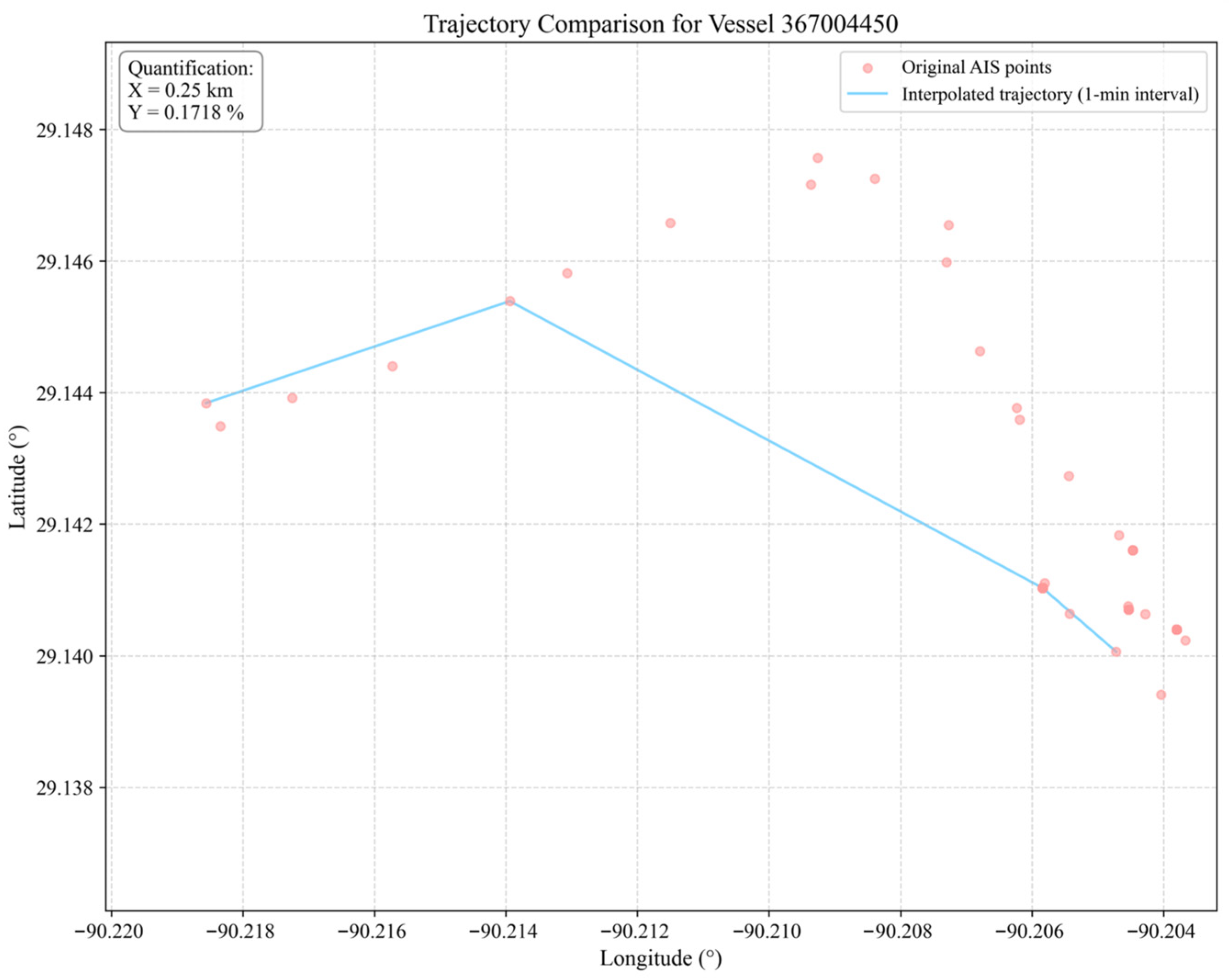
After completing the interpolation, invalid data points at the beginning and end of each vessel’s trajectory that could not be filled by interpolation were removed. The resulting time-series datasets, with uniform 1-min intervals, were stored separately as interpolated_ais_1min_region1.csv (Gulf of Mexico) and interpolated_ais_1min_region2.csv (Atlantic Coast). After NaN removal, Region 1 contained 106,110,280 valid records covering 1321 vessels, while Region 2 contained 116,465,520 records covering 1999 vessels. Figure 7 presents a comparison of trajectories before and after interpolation, using vessel MMSI 367004450 in Region 1 as an example. The average point-to-point displacement of the original AIS trajectory was approximately 0.25 km due to irregular sampling intervals. After linear interpolation to a uniform 1-min interval, the trajectory became temporally continuous and suitable for model input. The mean positional deviation introduced by the interpolation process was less than 0.1718% of the total trajectory length, confirming that the interpolation preserves the vessel’s original motion pattern while ensuring the data regularity required for model training.

3.1.2. Evaluation Metrics

To quantitatively evaluate the trajectory prediction performance of the proposed hybrid model, we select three core evaluation metrics based on the characteristics of ship trajectory data (longitude and latitude as spatial coordinates, speed as a scalar variable, and course as a periodic angular variable). These metrics are mean absolute error (MAE), root mean square error (RMSE), and the circular smallest angle difference. They assess the prediction accuracy of the model for different trajectory parameters. Smaller values of all metrics indicate better prediction performance.

$$\mathrm{MAE}={\displaystyle \frac{1}{n}}{\displaystyle \sum _{i=1}^n|\widehat{y}i-yi|}$$

(18)

$$\mathrm{RMSE}=\sqrt{{\displaystyle \frac{1}{n}}{\displaystyle \sum _{i=1}^n{({\widehat{\mathrm{y}}}_{\mathrm{i}}-{\mathrm{y}}_{\mathrm{i}})}^2}}$$

(19)

$$\mathrm{Angle} \mathrm{Error}={\displaystyle \frac{1}{n}}{\displaystyle \sum _{i=1}^{n}min(\left|\widehat{{\theta }_i}-{\theta }_i\right|,{360}^{\circ }-\left|\widehat{{\theta }_i}-{\theta }_i\right|)}$$

(20)

where $n$ is the number of samples in the test set; ${\widehat{y}}_i$ and $y_i$ are the predicted and true values of the i-th sample, respectively; ${\widehat{\theta }}_i$ and ${\theta }_i$ are the predicted and true courses of the i-th sample, respectively.

3.2. Prediction Results and Analysis

Comparison with existing methods. The baseline models selected for comparison—Transformer, CNN-BiLSTM-ATTENTION, and DenseNet-BiGRU-ATTENTION—were chosen because they represent the current mainstream of attention-enhanced hybrid architectures for ship trajectory prediction. These models share a similar design philosophy with the proposed MSC-BiLSTM-ATTENTION model, thereby ensuring a fair comparison under a unified experimental framework. All baseline models were re-implemented and trained on the same preprocessed AIS dataset under identical experimental conditions. Direct quantitative comparison with results reported in other published studies is complicated by inevitable differences in datasets, geographical regions, prediction horizons, and evaluation protocols. Nevertheless, the error reduction rates achieved by the proposed model align with the improvements reported in recent literature on attention-enhanced hybrid models, and on comparable baselines the MSC-BiLSTM-ATTENTION model consistently exhibits lower prediction errors.

After preprocessing, the segmentation method (L = 60 min, S = 120 min) produced 1,356,005 sub-segments for Region 1 (Gulf of Mexico) and 1,941,092 sub-segments for Region 2 (Atlantic Coast). Each sub-segment contains 60 consecutive time points.

Table 3. Clustering results.

Cluster ID	Region 1 (Gulf of Mexico)		Region 2 (Atlantic Coast)
	Sub-Segments	Vessels	Sub-Segments	Vessels
0	342,449	589	581,537	650
1	550,136	738	558,523	570
2	344,766	717	213,729	289

summarizes the number of sub-segments and distinct vessels assigned to each cluster after K-Means clustering, where Cluster 0 corresponds to low-density peripheral trajectories, Cluster 1 represents the dominant navigation pattern, and Cluster 2 contains trajectories with moderate density and distinct motion characteristics.

The number of clusters $K$ for Region 1 was determined through quantitative evaluation. As shown in

Table 4. Quantitative evaluation of clustering quality for different K values in Region 1.

K	WCSS	Silhouette Score	Davies Bouldin Index
3	18,386.14	0.3675	1.3621
4	15,528.64	0.2196	1.3167
5	14,056.42	0.2286	1.3999
6	12,994.34	0.2393	1.3447

, $K=3$ achieved the highest mean Silhouette Score (0.3675), indicating the best intra-cluster cohesion and inter-cluster separation. Although the Davies–Bouldin Index (DBI) reached its minimum at $K=4$ (1.3167), the value at $K=3$ (1.3621) was nearly identical and substantially lower than those for $K\ge 5$. Considering that the Silhouette Score drops sharply for $K\ge 4$ and that larger $K$ values risk fragmenting coherent trajectory patterns with insufficient training data per cluster, $K=3$ was selected as the optimal number of clusters, adequately representing the distinct navigation patterns in Region 1 without over-partitioning.

To evaluate the prediction performance of the proposed MSC-BiLSTM-ATTENTION model, we train and test the model on the three navigation pattern clusters (Cluster 0, Cluster 1, Cluster 2) for both regions independently, based on the preprocessing, segmentation, and clustering results described earlier. For each cluster, we construct input samples using a sliding window. We set the window length to 15 consecutive time steps.

Table 5. Features used for model input at each time step.

No.	Feature	Category
1	Longitude	Basic kinematic
2	Latitude	Basic kinematic
3	Speed Over Ground	Basic kinematic
4	Sin course	Angular encoding
5	Cos course	Angular encoding
6	Delta longitude	Motion change
7	Delta latitude	Motion change
8	Delta speed	Motion change
9	Delta course	Motion change
10	acceleration	Motion derivative
11	Turn rate	Motion derivative
12	Cumulative distance	Context
13	Elapsed time	Context
14	Moving average speed	Temporal context

lists the 14 features used at each time step. The 14 × 15 feature matrix is flattened into a 210-dimensional vector, which is then concatenated with the mean, standard deviation, maximum, and minimum of each feature computed across the 15 time steps, forming a final 266-dimensional input vector. The corresponding output is a 14-dimensional vector comprising the same features at the next time step. We split the dataset chronologically into training and test sets (80%/20%). We train the model using the Adam optimizer with a learning rate of 0.001 and a batch size of 128. The loss function is mean squared error (MSE). We also employ a learning rate scheduler and early stopping.

Table 6. Parameter settings for the MSC-BiLSTM-ATTENTION model.

Layer Name	Parameter Setting
Multi-Scale Convolution	3 branches, kernel sizes = 2/3/4, filters = 64, padding = 1 (kernel 2, 3)/2 (kernel 4)
Activation (MSC)	ReLU
Pooling (MSC)	AdaptiveMaxPool1d (output size = 1)
BiLSTM	hidden size = 256, layers = 1, bidirectional
Attention	self-attention, input dim = 512
Dropout	dropout rate = 0.3
Num epochs	150
Batch size	128
Learning rate	0.001
Optimizer	Adam
Loss function	MSE
Gradient clipping	1.0
Early stopping patience	15

summarizes the detailed parameter settings of the proposed model. The MSC module consists of three parallel one-dimensional convolutional branches. Their kernel sizes are 2, 3, and 4, with 64 filters each. This design captures local trajectory features at multiple temporal scales. The BiLSTM module uses a single-layer bidirectional structure with a hidden size of 256. The self-attention mechanism receives the concatenated BiLSTM outputs (dimension 512) and adaptively assigns weights to key features. The model is trained for up to 150 epochs with a batch size of 128. The Adam optimizer is adopted with a learning rate of 0.001. Early stopping with a patience of 15 epochs and gradient clipping (max norm 1.0) are applied to ensure training stability.

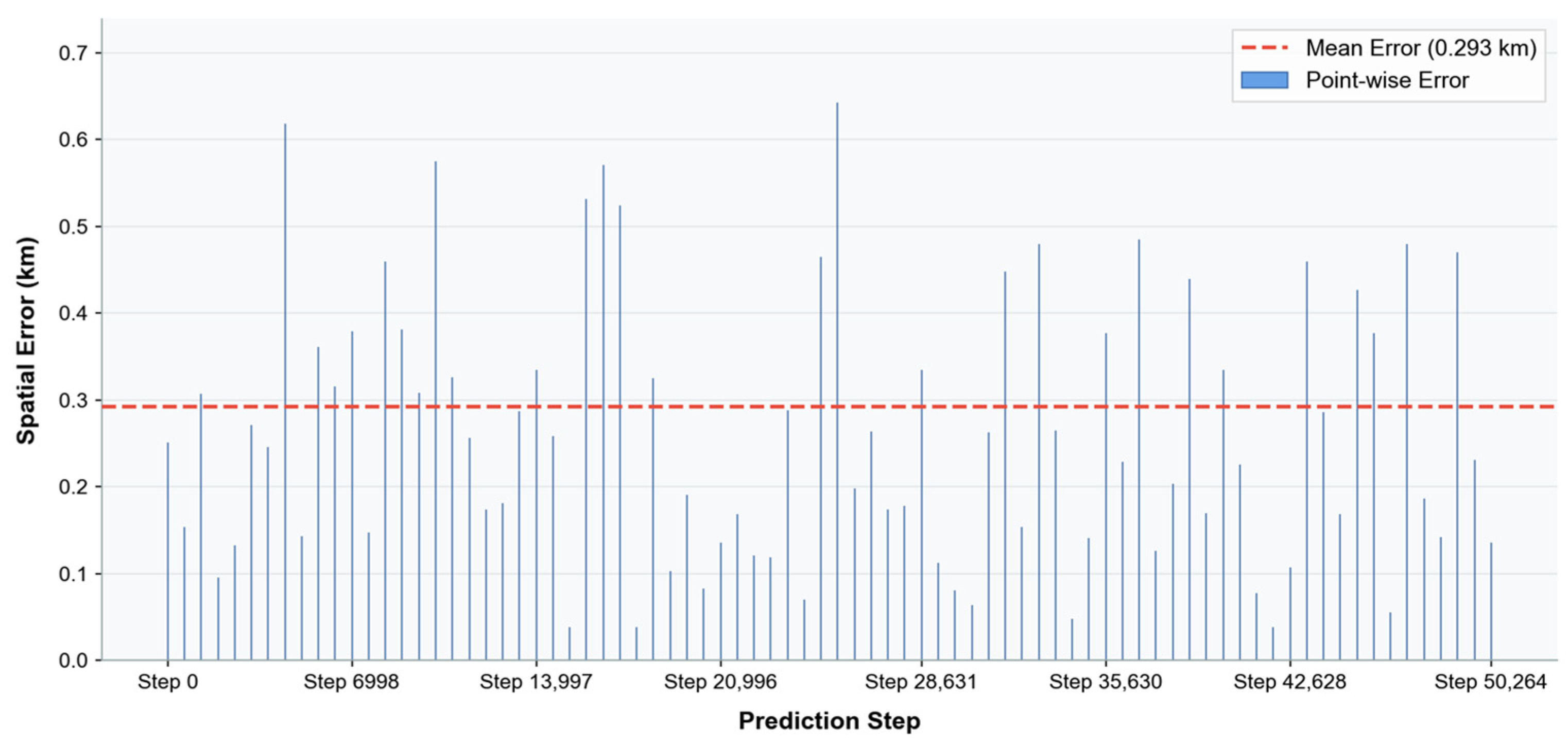
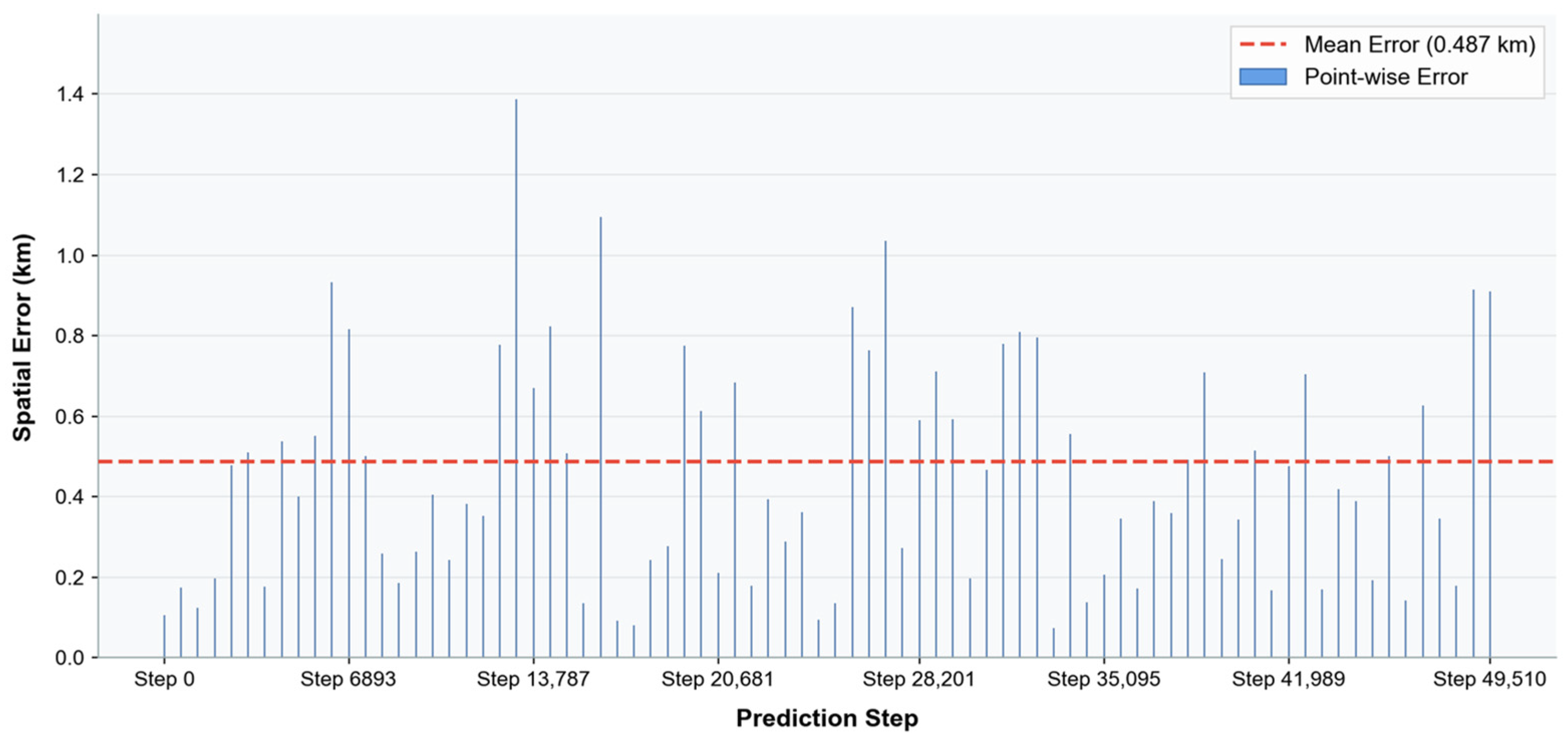
Figure 8 and Figure 9 present the spatial prediction error of the MSC-BiLSTM-ATTENTION model on representative test samples from the Gulf of Mexico and the Atlantic Coast, respectively. In each figure, the point-wise Haversine distance between the predicted and true positions is evaluated at 80 uniformly sampled prediction steps spanning the entire trajectory, with the mean error indicated by a dashed reference line. In the Gulf of Mexico (Figure 8), the point-wise error fluctuates between approximately 0.15 km and 0.50 km, with the majority of steps exhibiting errors below 0.25 km and no clear long-term drift. On the Atlantic Coast (Figure 9), the error remains within a narrow band of 0.10–0.25 km across the displayed steps, and no significant spikes are observed. The overall mean prediction error is approximately 0.27 km and 0.24 km for the two regions, respectively. These values are substantially smaller than the standard ship domain in open waters. According to Hörteborn et al., the ship domain in open waters forms an ellipse with half-axis radii of 0.9 and 0.45 nautical miles (approximately 1650 m and 830 m, respectively) [41]. The observed errors are therefore an order of magnitude smaller than the established safety area that vessels maintain around themselves. This level of accuracy can provide reliable decision support for vessel traffic service (VTS) operators, reduce false collision alarms, and improve traffic flow efficiency in busy waterways. Although occasional larger deviations occur during abrupt maneuvers (especially in the Gulf of Mexico dataset), the model quickly recovers to a low error level, demonstrating good adaptability. Furthermore, these errors are consistently lower than those of the Transformer-based TPTrans model proposed by Wang et al. [9], which relies solely on self-attention mechanisms without the multi-scale convolutional feature extraction and bidirectional temporal modeling that enable the proposed MSC-BiLSTM-ATTENTION model to capture finer spatial details across diverse waterway conditions.

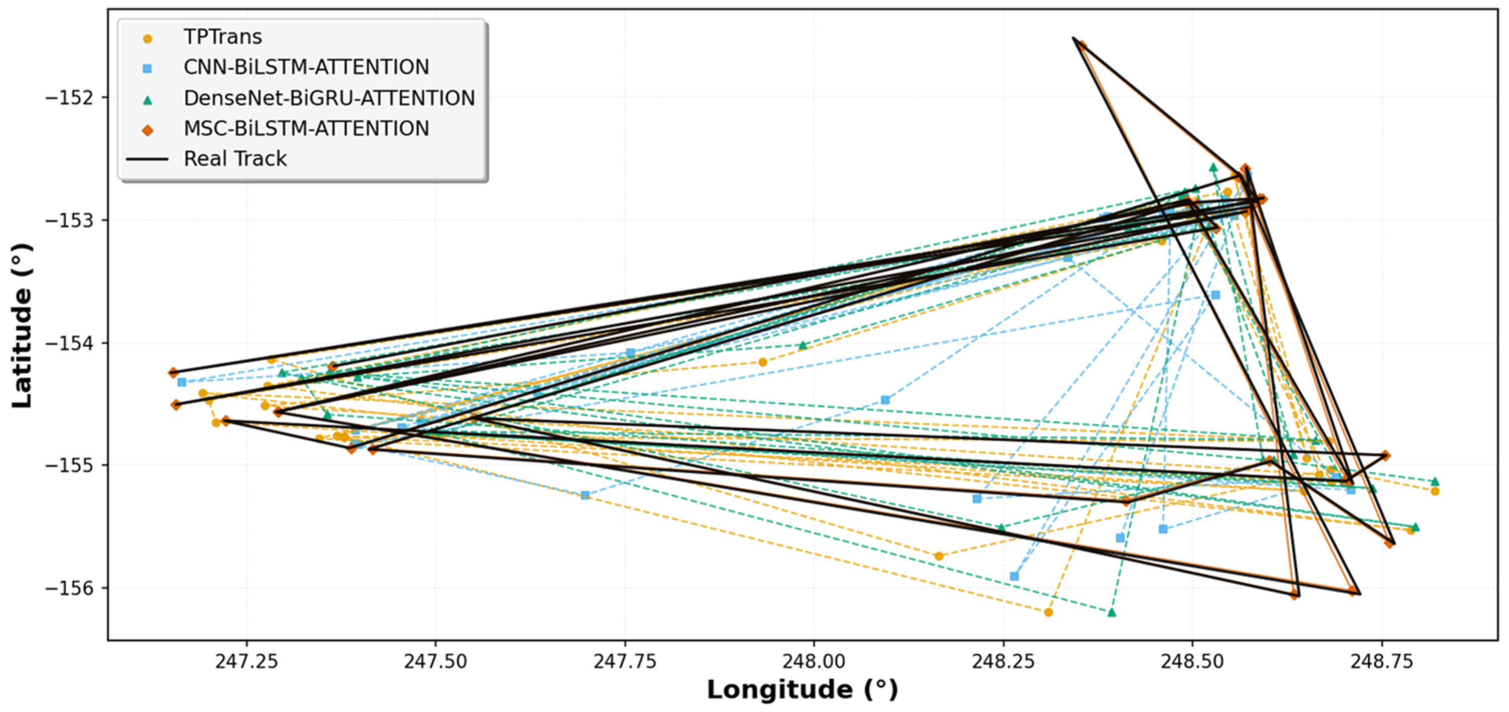
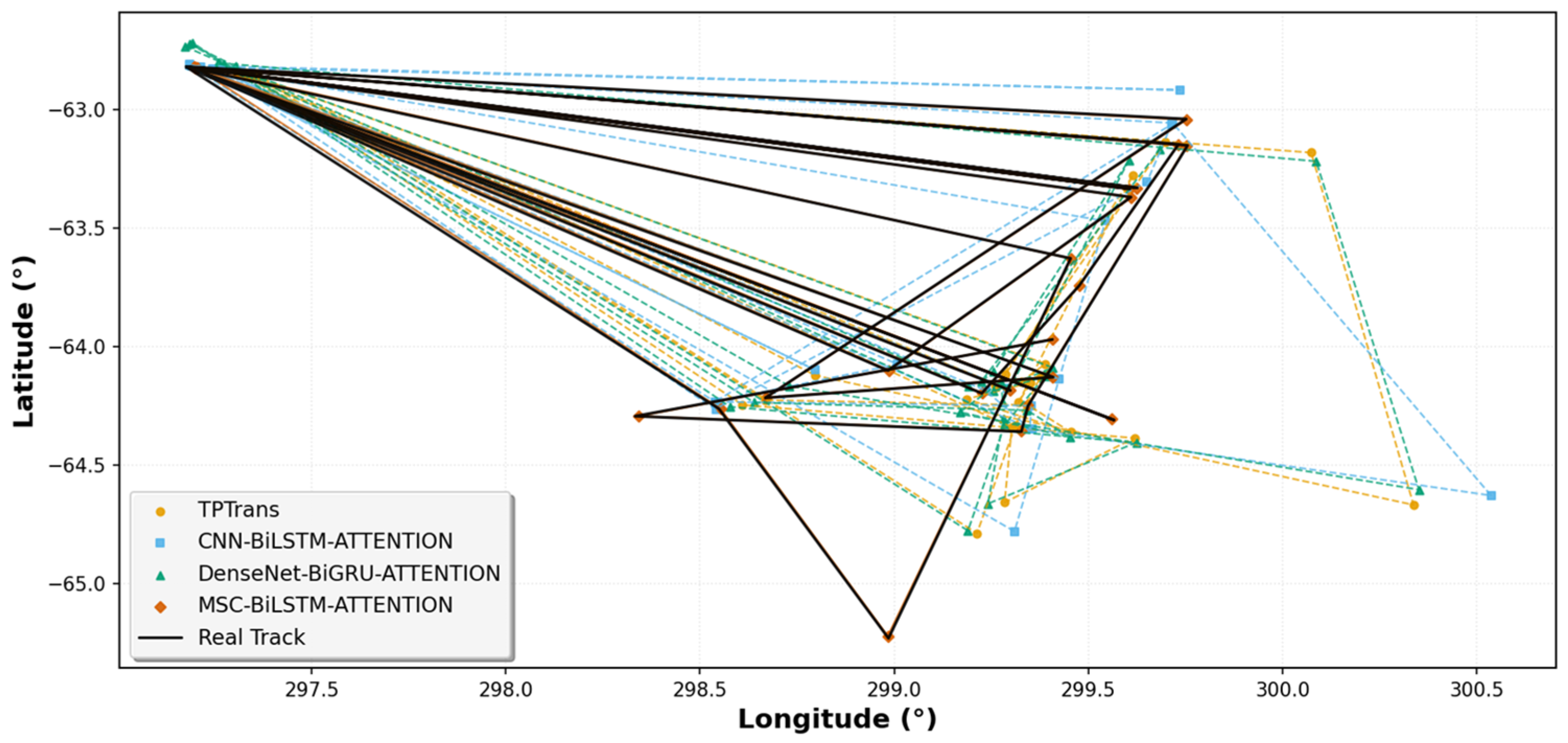
Figure 10 and Figure 11 present the trajectory prediction results of the four compared models on the Gulf of Mexico and Atlantic Coast test sets, respectively. In each figure, 30 time steps with the largest prediction disagreement among all models are selected for visualization, and the predicted trajectories are plotted against the true trajectory. In both regions, the predicted trajectory of the proposed MSC-BiLSTM-ATTENTION model consistently exhibits the closest agreement with the true trajectory, with only slight deviations visible at local turning points, confirming its robust spatial accuracy across both open-water and confined estuarine environments. The Transformer and CNN-BiLSTM-ATTENTION models show systematic parallel offsets, while the DenseNet-BiGRU-ATTENTION model shows the largest deviations. These differences can be attributed to the synergistic design of the proposed model: the MSC module captures multi-scale local features, the BiLSTM preserves bidirectional temporal context, and the self-attention mechanism dynamically emphasizes critical information for trajectory prediction.

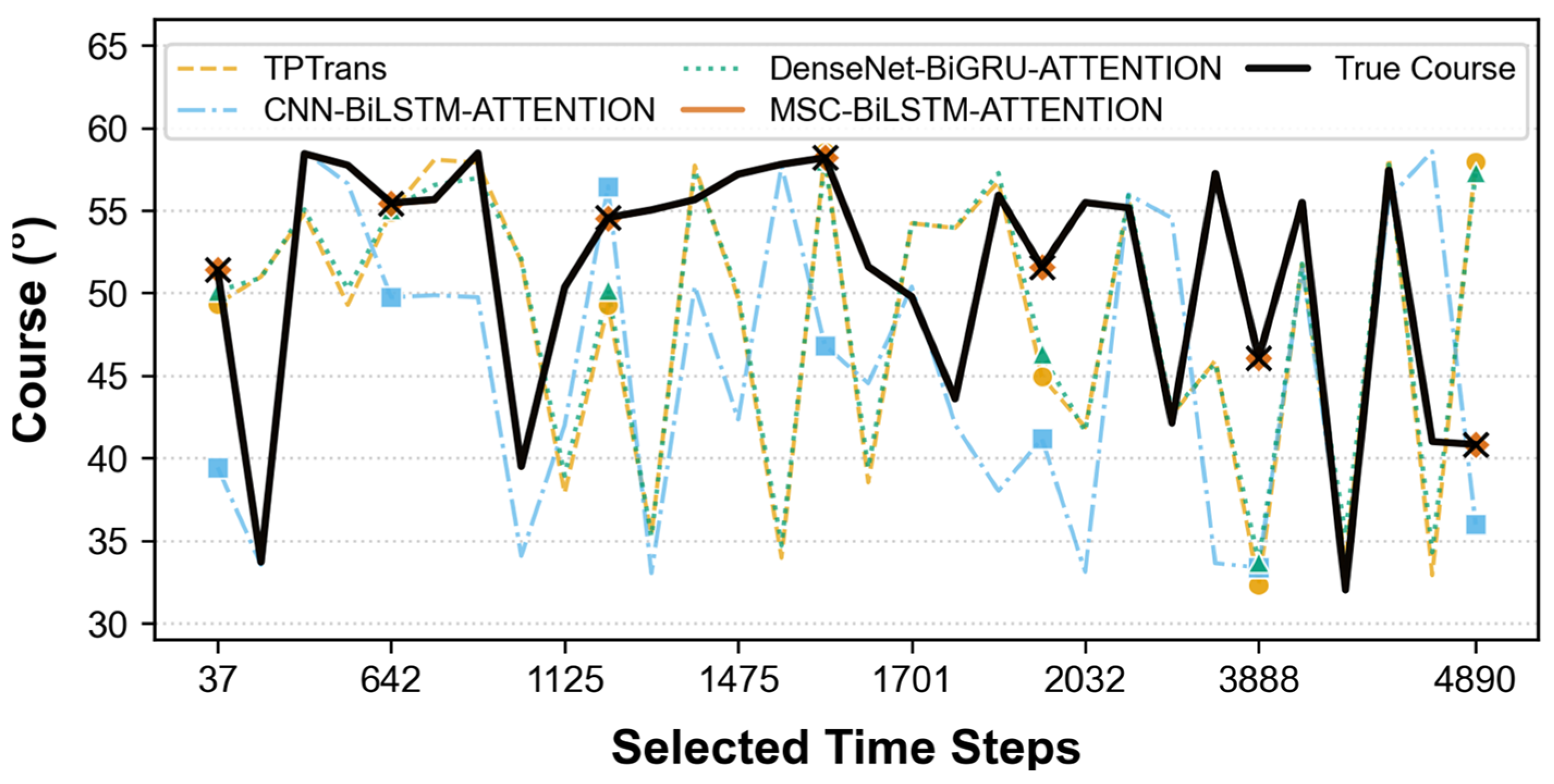
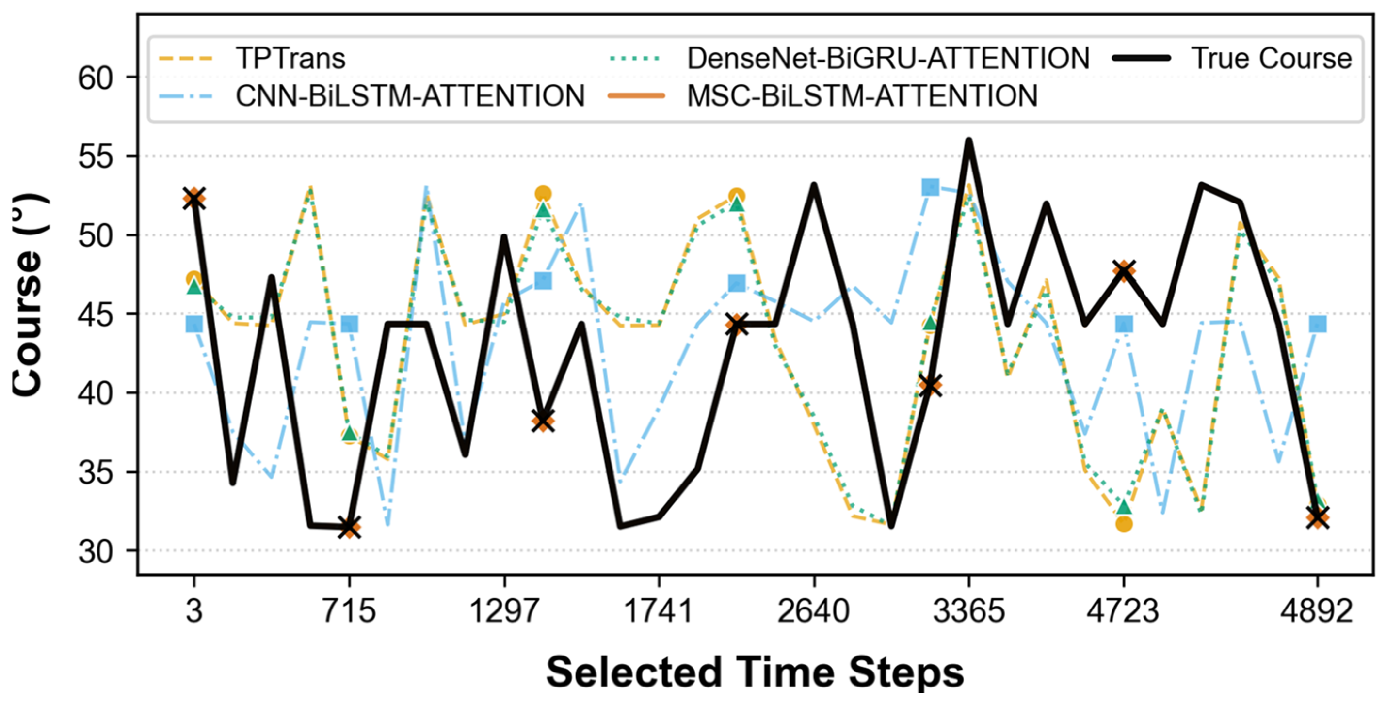
Figure 12 and Figure 13 present the course prediction results on the same set of 30 high-disagreement time steps selected for the trajectory comparison. In both regions, the proposed MSC-BiLSTM-ATTENTION model achieves the best overall consistency with the true course, maintaining closer alignment and recovering more quickly from deviations during rapid heading changes. The DenseNet-BiGRU-ATTENTION and CNN-BiLSTM-ATTENTION models exhibit larger and more persistent deviations, and their predictions often conflate gradual course adjustments with abrupt turns. This superior course tracking capability stems from the same combination of MSC, BiLSTM, and self-attention, which together provide multi-granularity temporal features, bidirectional context integration, and adaptive weighting of recent maneuvering information.

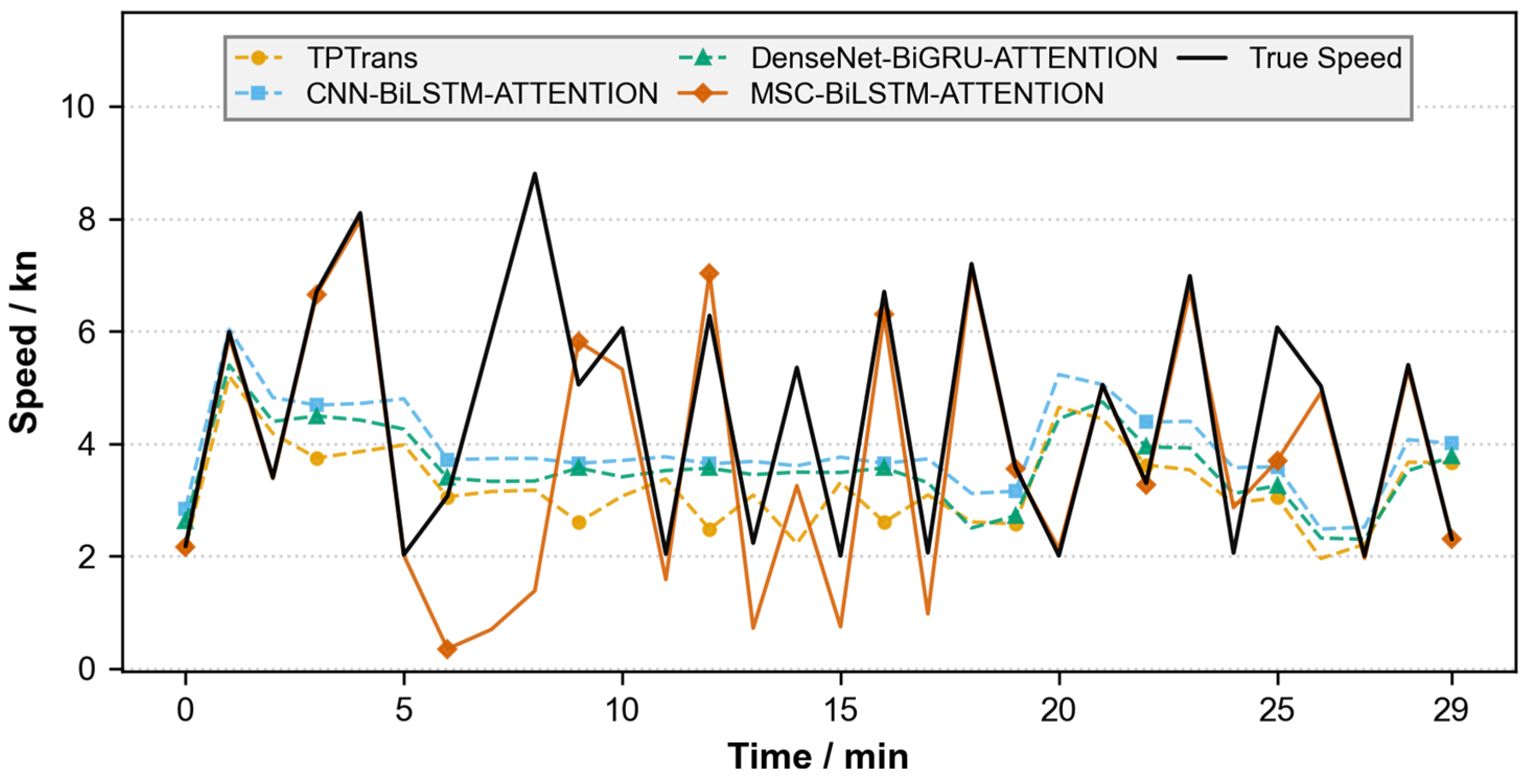
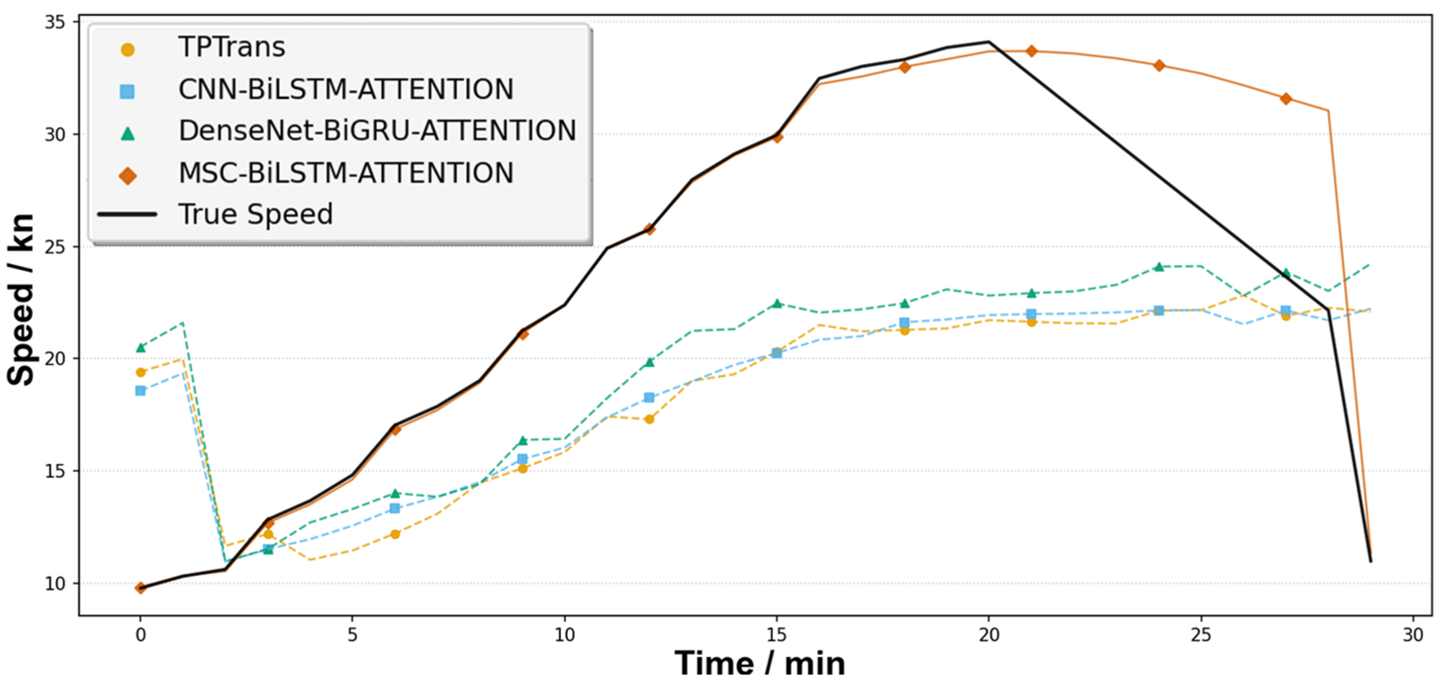
Figure 14 and Figure 15 present the speed prediction results, also using the 30 time steps with the largest prediction disagreement among all models (the same selection strategy as for trajectory and course). In both regions, the proposed MSC-BiLSTM-ATTENTION model consistently achieves the closest agreement with the true speed, accurately capturing the overall trend as well as local variations without noticeable lag or systematic overshoot. The CNN-BiLSTM-ATTENTION model tends to underestimate speed during rapid changes, while the DenseNet-BiGRU-ATTENTION model frequently overestimates the true values, and the Transformer model yields intermediate accuracy but lacks fine-grained responsiveness. This superior speed tracking capability can be attributed to the combined effect of the MSC module, the BiLSTM, and the self-attention mechanism, which together enable the model to extract multi-temporal features, integrate full temporal context, and rapidly adapt to acceleration or deceleration events.

To further quantify the model advantages, we calculate the mean absolute error (MAE) and root mean square error (RMSE) for longitude, latitude, course, and speed on the test set for each model.

Table 7. Error statistics of compared models for the Gulf of Mexico dataset.

Model	MSC-BiLSTM-ATTENTION		Transformer		CNN-BiLSTM-ATTENTION		DenseNet-BiGRU-ATTENTION
Indicator	MAE	RMSE	MAE	RMSE	MAE	RMSE	MAE	RMSE
Longitude	0.001955	0.003111	0.026751	0.035283	0.005179	0.008466	0.042673	0.054862
Latitude	0.003748	0.007356	0.053389	0.068230	0.012753	0.020571	0.076569	0.096096
Course	0.027009	0.164246	0.357424	0.489895	0.115492	0.384930	0.548571	0.693452
Speed of the ship	0.000021	0.000042	0.000333	0.000428	0.000091	0.000121	0.000218	0.000307

and

Table 8. Error statistics of compared models for the Atlantic Coast dataset.

Model	MSC-BiLSTM-ATTENTION		Transformer		CNN-BiLSTM-ATTENTION		DenseNet-BiGRU-ATTENTION
Indicator	MAE	RMSE	MAE	RMSE	MAE	RMSE	MAE	RMSE
Longitude	0.002450	0.005402	0.030643	0.041781	0.020919	0.025799	0.030402	0.038677
Latitude	0.002172	0.003329	0.022686	0.029228	0.015156	0.019178	0.019925	0.028456
Course	0.025211	0.133512	0.191404	0.356881	0.099862	0.249279	0.383973	0.488384
Speed of the ship	0.000032	0.000051	0.000439	0.000554	0.000110	0.000151	0.000260	0.000341

present the error results.

The quantitative error statistics in Table 7 and Table 8 confirm that the proposed MSC-BiLSTM-ATTENTION model consistently achieves the lowest MAE and RMSE across all four core features on both datasets. In the Gulf of Mexico, the model reduces speed MAE by 76.9% and speed RMSE by 65.3% compared with the strongest baseline; on the Atlantic Coast, corresponding reductions of 70.9% and 66.2% are achieved. Similar substantial improvements are observed in longitude, latitude, and course prediction across both regions. Together with the qualitative visual comparisons, these results demonstrate the superior accuracy and robust generalisation capability of the proposed model across different waterway types.

3.3. Ablation Study

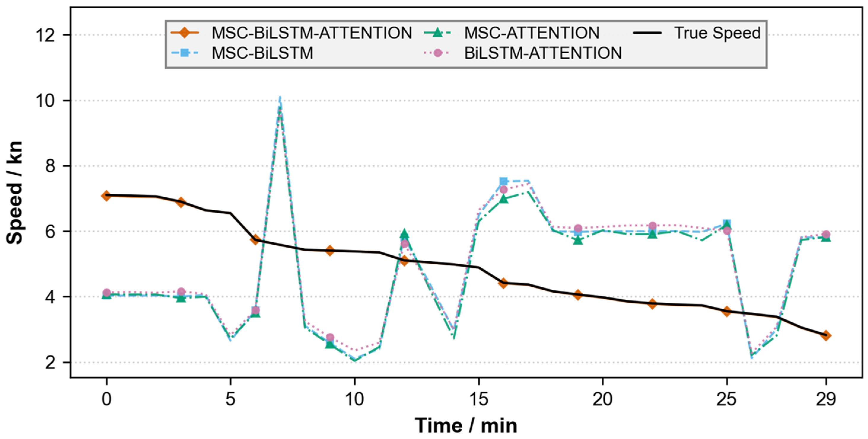
To further validate the effectiveness of each module in the proposed MSC-BiLSTM-ATTENTION model, which integrates multi-scale convolution and an adaptive attention mechanism, we design an ablation study. We compare the full model with three variants: the MSC-BiLSTM model (without the attention mechanism), the BiLSTM-ATTENTION model (without the multi-scale convolution module), and the MSC-ATTENTION model (without the BiLSTM temporal modeling module). This comparison systematically verifies the contribution of the three core components—multi-scale convolution, bidirectional LSTM temporal modeling, and the attention mechanism—to the model’s prediction performance. We keep the experimental environment, dataset, and evaluation metrics consistent with those described in previous sections to ensure comparability and reliability of the results.

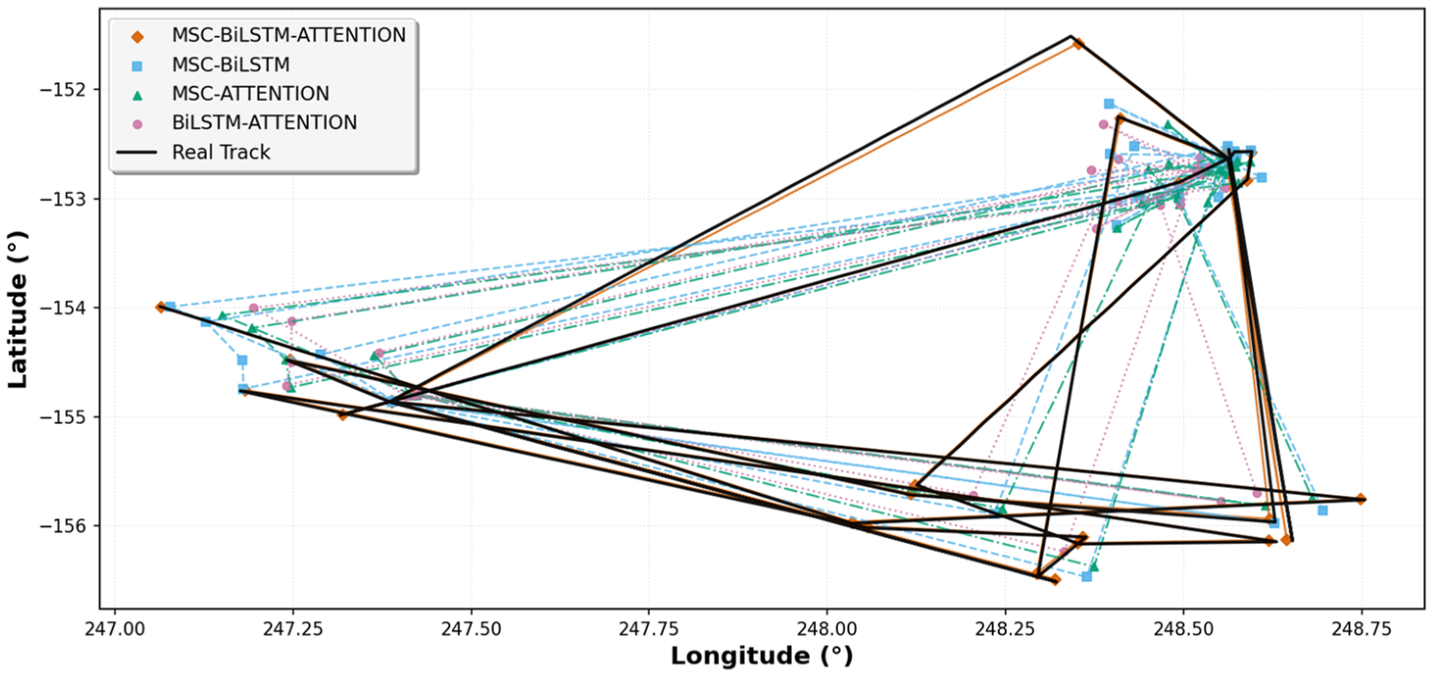
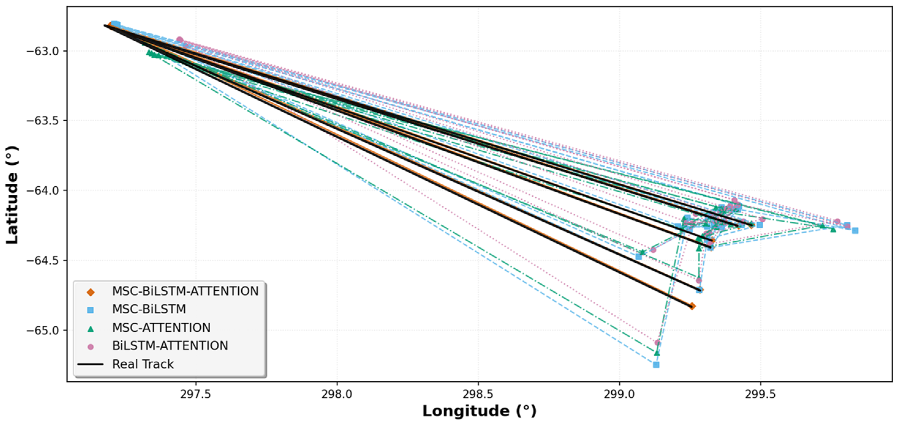
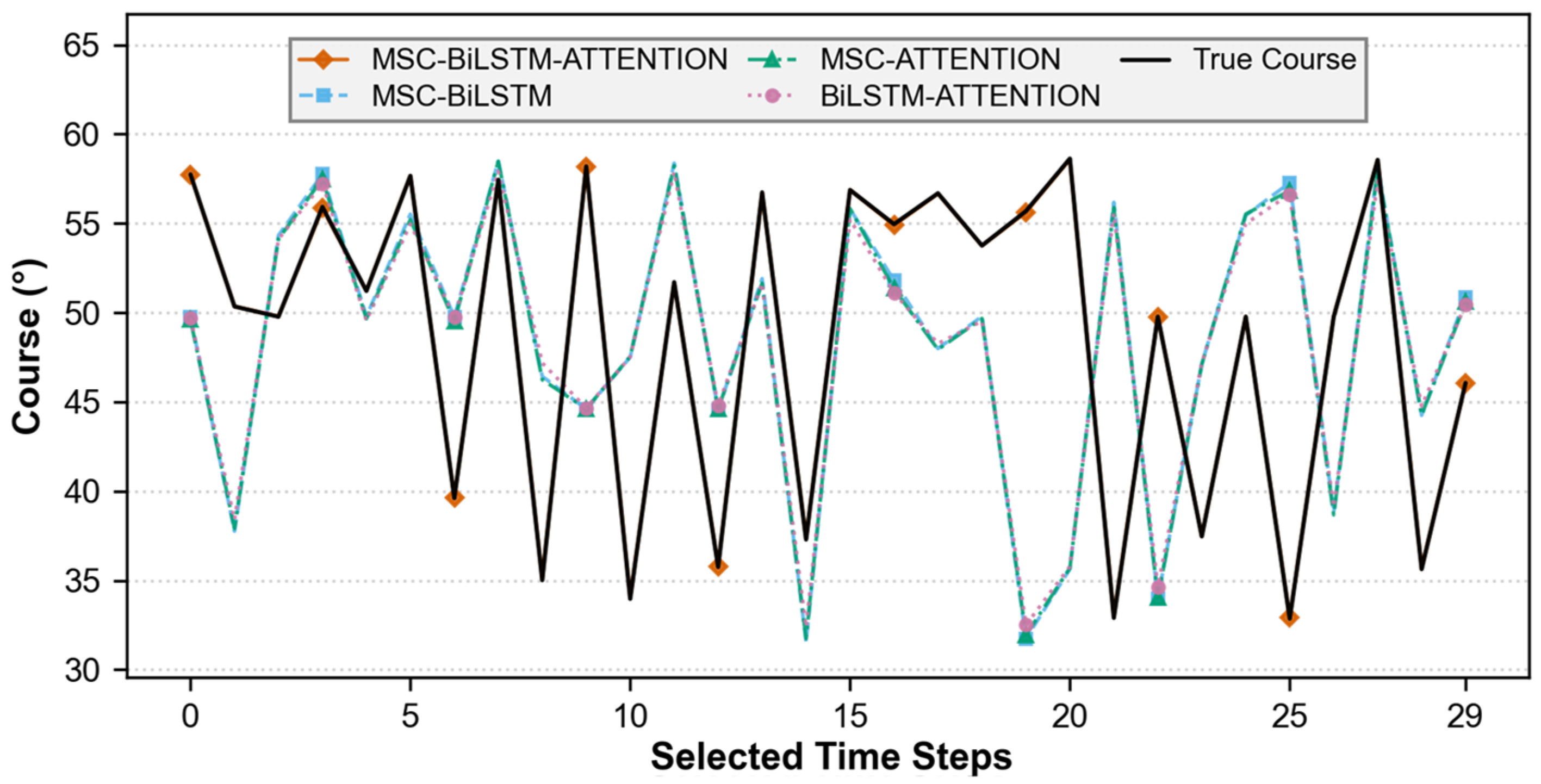
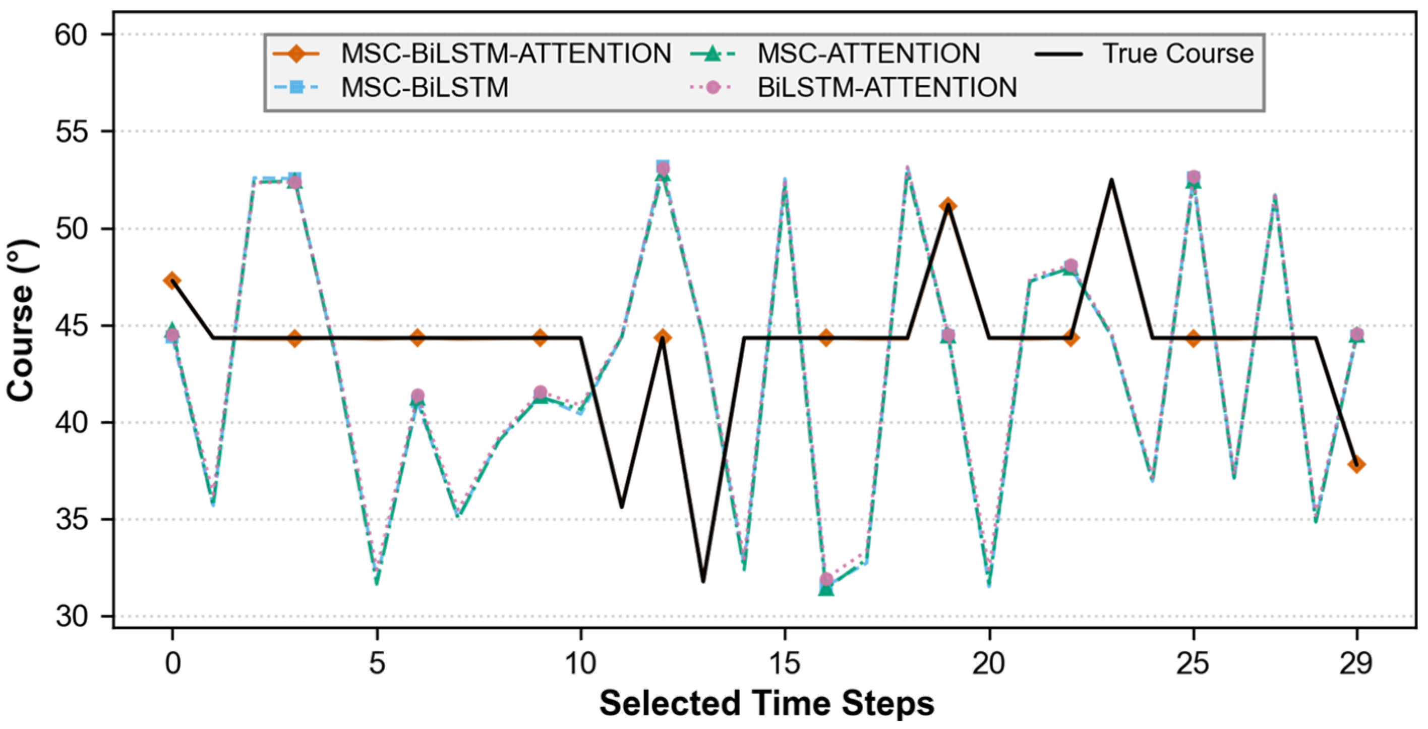
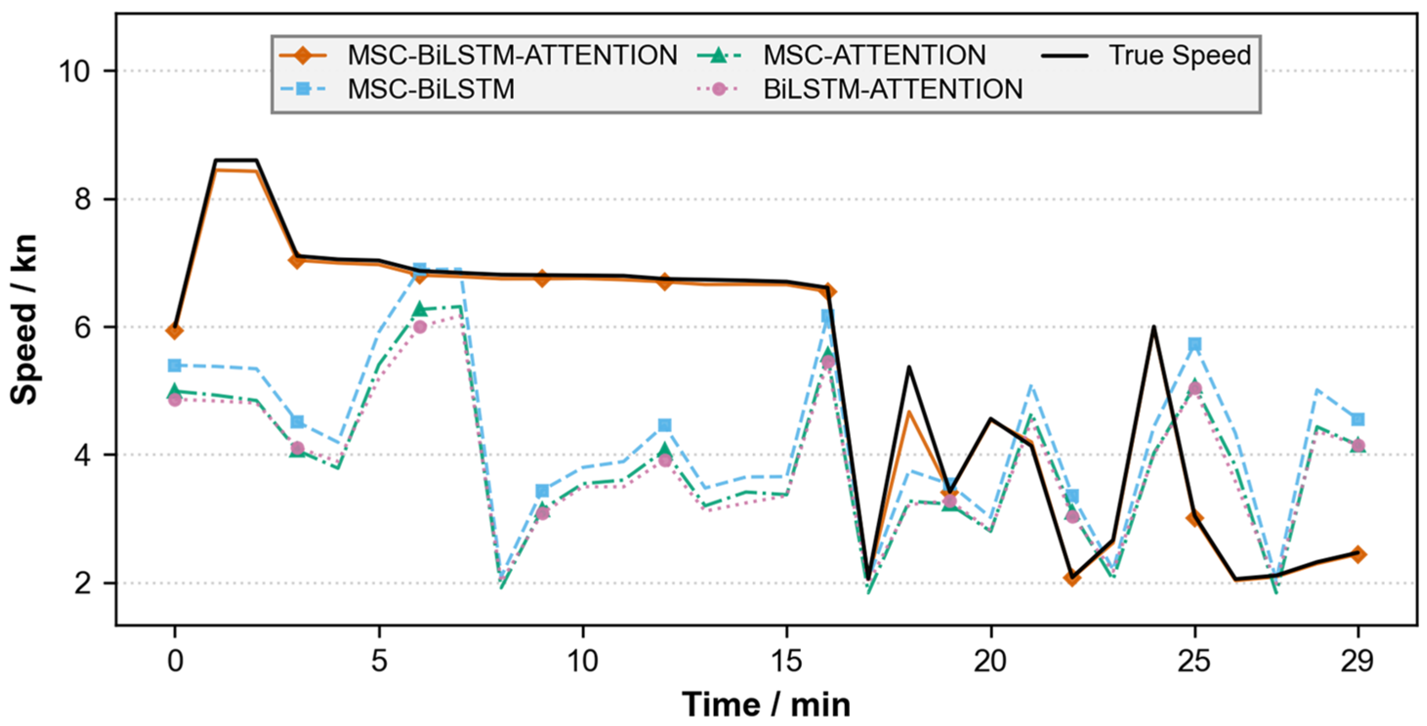
We conduct a systematic comparison from three dimensions: spatial trajectory shape, time-series course over ground (COG), and speed over ground (SOG). Figure 16, Figure 17, Figure 18, Figure 19, Figure 20 and Figure 21 and

Table 9. Feature error statistics of ablation study models in the Gulf of Mexico.

Model	MSC-BiLSTM		MSC-ATTENTION		BiLSTM-ATTENTION
Indicator	MAE	RMSE	MAE	RMSE	MAE	RMSE
Longitude	0.002983	0.004752	0.019966	0.026293	0.037250	0.044439
Latitude	0.006584	0.010161	0.042853	0.052328	0.044933	0.057729
Course	0.043842	0.166711	0.216854	0.328008	0.294230	0.447276
Speed of the ship	0.000023	0.000054	0.000220	0.000261	0.000266	0.000320

and

Table 10. Feature error statistics of ablation study models on the Atlantic Coast.

Model	MSC-BiLSTM		MSC-ATTENTION		BiLSTM-ATTENTION
Indicator	MAE	RMSE	MAE	RMSE	MAE	RMSE
Longitude	0.004115	0.006503	0.030510	0.043672	0.032153	0.051364
Latitude	0.002899	0.004141	0.026466	0.034271	0.029936	0.038587
Course	0.048056	0.237945	0.219102	0.380815	0.361175	0.493571
Speed of the ship	0.000058	0.000092	0.000390	0.000458	0.000535	0.000594

present the results.

Figure 16 and Figure 17 present the trajectory prediction results of the ablation models on the Gulf of Mexico and Atlantic Coast, respectively. In both regions, the full MSC-BiLSTM-ATTENTION model produces predicted trajectories that most closely match the true tracks in overall direction, turning points, and local details. The MSC-BiLSTM variant (without attention) exhibits only minor deviations, whereas the MSC-ATTENTION and BiLSTM-ATTENTION variants show significantly larger spatial errors and trajectory divergence, especially in complex segments.

Figure 18 and Figure 19 show the corresponding course prediction results. The full model accurately tracks rapid heading changes and quickly recovers from transient deviations. The MSC-BiLSTM model shows only slight oscillations, while the MSC-ATTENTION and BiLSTM-ATTENTION variants exhibit persistent overshoot and lag, indicating that neither multi-scale convolution nor bidirectional temporal modeling alone is sufficient for capturing fine-grained heading dynamics.

Figure 20 and Figure 21 display the speed prediction comparisons. The full model closely follows the true speed variations, including rapid acceleration and deceleration phases. The MSC-BiLSTM model maintains reasonable tracking, whereas the MSC-ATTENTION and BiLSTM-ATTENTION variants show conspicuous delay and systematic bias, respectively, during sharp speed changes.

The quantitative error statistics in Table 9 and Table 10 strongly corroborate these visual observations. On the Gulf of Mexico dataset (Table 9), removing the attention mechanism (MSC-BiLSTM) increases speed MAE by approximately 10% and speed RMSE by roughly 29%, representing only moderate degradation. However, further removing the MSC module (BiLSTM-ATTENTION) causes speed errors to surge by more than an order of magnitude, confirming that multi-scale feature extraction is the most critical component for speed prediction. A similar pattern is observed on the Atlantic Coast dataset (Table 10), where the same architectural dependencies are consistently reproduced.

More broadly, the ablation results reveal a clear hierarchical structure among the three modules. Multi-scale convolution and bidirectional LSTM together form the foundational backbone of the model: when either is removed, performance collapses across all four output features. The self-attention mechanism acts as a refinement layer: it provides additional but comparatively smaller gains, particularly for course and trajectory prediction. This asymmetry confirms that robust local feature extraction at multiple temporal granularities and bidirectional context integration are indispensable for modeling complex vessel dynamics, while the attention module further enhances accuracy by adaptively emphasizing critical temporal segments.

In summary, both the visual and quantitative ablation results confirm that the synergistic combination of MSC, BiLSTM, and self-attention contributes significantly to the model’s state-of-the-art performance across two distinct waterway types.

4. Conclusions

To improve the accuracy and adaptability of ship trajectory prediction in complex maritime scenarios, this paper addresses the limitations of traditional prediction models in processing AIS data, including insufficient local feature extraction, limited long-term dependency capture, and inflexible feature weight allocation. We propose an MSC-BiLSTM prediction model that integrates trajectory clustering and an adaptive attention mechanism. The main research work and conclusions are as follows:

• To reduce the interference of data heterogeneity on prediction, the method removes outliers, applies linear interpolation for missing values, and normalizes the raw AIS data. It then uses a fixed-time sliding window to generate uniform sub-segments. It fuses temporal and statistical features into a combined vector. Finally, it applies K-Means clustering to group sub-segments with similar navigation characteristics into the same cluster. This provides high-quality input data for the subsequent prediction model.
• To address insufficient feature extraction and inflexible weight allocation in existing models, this paper designs an MSC BiLSTM network architecture that integrates an adaptive attention mechanism. The MSC uses parallel convolutional kernels of different sizes to extract multi scale local deep features from AIS data, such as sudden speed changes and course turns. The BiLSTM captures temporal dependencies in the trajectory data from both forward and backward directions. The self attention mechanism then dynamically allocates feature weights to strengthen the contribution of key features to trajectory prediction.
• Experimental results based on AIS data from both the Gulf of Mexico and the U.S. Atlantic Coast, covering four distinct seasons, demonstrate that the proposed MSC-BiLSTM-ATTENTION model consistently outperforms three comparison models (Transformer, CNN-BiLSTM-ATTENTION, and DenseNet-BiGRU-ATTENTION) across all four core features (longitude, latitude, speed, course) in terms of MAE and RMSE. On the Gulf of Mexico dataset, the proposed model reduces speed MAE by 76.9% and speed RMSE by 65.3% relative to the strongest baseline; on the Atlantic Coast dataset, corresponding reductions of 70.9% and 66.2% are achieved. Substantial improvements are also observed in longitude, latitude, and course prediction across both regions. Ablation studies further confirm that removing any single module (multi-scale convolution, BiLSTM, or self-attention) leads to significant error increases, with the MSC and BiLSTM modules forming the foundational backbone and the attention mechanism serving as an effective refinement layer. These results, obtained from two geographically distinct waterways with different traffic patterns, fully validate the effectiveness, superiority, and cross-region generalisation capability of the proposed hybrid architecture.

Although the proposed model achieves strong performance, two main limitations should be noted. First, the current results are reported as single-point estimates without statistical validation (e.g., standard deviations, confidence intervals, or significance tests), and the computational cost of the model has not been systematically compared with baselines in terms of parameters, training time, and inference latency. Second, the model relies solely on AIS kinematic data and does not incorporate environmental factors such as wind, waves, and currents, which could further improve prediction robustness in adverse conditions. Addressing these issues will strengthen the empirical foundation of the proposed approach and facilitate its practical deployment.

References

1. UNCTAD. Review of Maritime Transport 2025: Staying the Course in Turbulent Waters; United Nations Conference on Trade and Development: Geneva, Switzerland, 2025. [Google Scholar]
2. Transportation Safety Board of Canada. Marine Transportation Occurrences in 2024. Marine Safety Statistical Summary; Transportation Safety Board of Canada: Gatineau, QC, Canada, 2025.
3. Jiao, H.; Li, H.; Lam, J.S.L.; Gao, X.; Yang, Z. Multi-factor influence-based ship trajectory prediction analysis via deep learning. J. Mar. Eng. Technol. 2025, 24, 123–135. [Google Scholar] [CrossRef] [Scilit]
4. Evmides, N.; Michaelides, M.P.; Herodotou, H. Vessel Trajectory Prediction with Deep Learning: Temporal Modeling and Operational Implications. J. Mar. Sci. Eng. 2025, 13, 1439. [Google Scholar] [CrossRef] [Scilit]
5. Huang, F.; Liu, Z.; Li, X.; Mou, F.; Li, P.; Fan, Z. Vessel trajectory prediction based on AIS data: Dual-path spatial–temporal attention network with multi-attribute information. J. Mar. Sci. Eng. 2024, 12, 2031. [Google Scholar] [CrossRef] [Scilit]
6. Chen, X.; Wei, C.; Zhou, G.; Wu, H.; Wang, Z.; Biancardo, S.A. Automatic Identification System (AIS) Data Supported Ship Trajectory Prediction and Analysis via a Deep Learning Model. J. Mar. Sci. Eng. 2022, 10, 1314. [Google Scholar] [CrossRef] [Scilit]
7. Cen, J.; Li, J.; Liu, X.; Chen, J.; Li, H.; Huang, W.; Zeng, L.; Kang, J.-X.; Ke, S. A Hybrid Prediction Model of Vessel Trajectory Based on Attention Mechanism and CNN-GRU. Proc. Inst. Mech. Eng. Part M J. Eng. Marit. Environ. 2024, 238, 809–823. [Google Scholar] [CrossRef] [Scilit]
8. Tong, X.; Chen, X.; Sang, L.; Yan, A.; Wu, Q. Vessel trajectory prediction in curving channel of inland river. In Proceedings of the 2015 3rd International Conference on Transportation Information and Safety, Wuhan, China, 25–28 June 2015; pp. 706–714. [Google Scholar] [CrossRef] [Scilit]
9. Wang, W.; Xiong, W.; Ouyang, X.; Chen, L. TPTrans: Vessel trajectory prediction model based on Transformer using AIS data. ISPRS Int. J. Geo-Inf. 2024, 13, 400. [Google Scholar] [CrossRef] [Scilit]
10. Qiang, H.; Guo, Z.; Chu, Z.; Xie, S.; Peng, X. Motion-Inspired Spatial–Temporal Transformer for accurate vessel trajectory prediction. Eng. Appl. Artif. Intell. 2025, 148, 110391. [Google Scholar] [CrossRef] [Scilit]
11. Fossen, S.; Fossen, T.I. Extended Kalman Filter Design and Motion Prediction of Ships Using Live Automatic Identification System (AIS) Data. In Proceedings of the 2018 2nd European Conference on Electrical Engineering and Computer Science (EECS), Bern, Switzerland, 20–22 December 2018; pp. 464–470. [Google Scholar] [CrossRef] [Scilit]
12. Zhang, X.; Liu, J.; Gong, P.; Chen, C.; Han, B.; Wu, Z. Trajectory prediction of seagoing ships in dynamic traffic scenes via a gated spatio-temporal graph aggregation network. Ocean Eng. 2023, 287, 115886. [Google Scholar] [CrossRef] [Scilit]
13. Bao, K.; Bi, J.; Gao, M.; Sun, Y.; Zhang, X.; Zhang, W. An Improved Ship Trajectory Prediction Based on AIS Data Using MHA-BiGRU. J. Mar. Sci. Eng. 2022, 10, 804. [Google Scholar] [CrossRef] [Scilit]
14. Wang, X.; Xiao, Y. A Deep Learning Model for Ship Trajectory Prediction Using Automatic Identification System (AIS) Data. Information 2023, 14, 212. [Google Scholar] [CrossRef] [Scilit]
15. Wu, Y.; Yv, W.; Zeng, G.; Shang, Y.; Liao, W. GL-STGCNN: Enhancing Multi-Ship Trajectory Prediction with MPC Correction. J. Mar. Sci. Eng. 2024, 12, 882. [Google Scholar] [CrossRef] [Scilit]
16. Dong, X.; Raja, S.S.; Zhang, J.; Wang, L. Ship Trajectory Prediction Based on CNN-MTABiGRU Model. IEEE Access 2024, 12, 115306–115318. [Google Scholar] [CrossRef] [Scilit]
17. Yang, C.H.; Wu, C.H.; Shao, J.C.; Wang, Y.C.; Hsieh, C.M. AIS-Based Intelligent Vessel Trajectory Prediction Using Bi-LSTM. IEEE Access 2022, 10, 24302–24315. [Google Scholar] [CrossRef] [Scilit]
18. Jiang, D.; Shi, G.; Li, N.; Ma, L.; Li, W.; Shi, J. TRFM-LS: Transformer-Based Deep Learning Method for Vessel Trajectory Prediction. J. Mar. Sci. Eng. 2023, 11, 880. [Google Scholar] [CrossRef] [Scilit]
19. Chen, J.; Zhang, J.; Chen, H.; Zhao, Y.; Wang, H. A TDV Attention-Based BiGRU Network for AIS-Based Vessel Trajectory Prediction. iScience 2023, 26, 106383. [Google Scholar] [CrossRef] [Scilit]
20. Liu, W.; Cao, Y. Research on Offshore Vessel Trajectory Prediction Based on PSO-CNN-RGRU-Attention. Appl. Sci. 2025, 15, 3625. [Google Scholar] [CrossRef] [Scilit]
21. Zhang, X.; Liu, J.; Chen, C.; Wei, L.; Wu, Z.; Dai, W. Goal-Driven Long-Term Marine Vessel Trajectory Prediction with a Memory-Enhanced Network. Expert Syst. Appl. 2025, 263, 125715. [Google Scholar] [CrossRef] [Scilit]
22. Bi, J.; Gao, M.; Bao, K.; Zhang, W.; Zhang, X.; Cheng, H. A CNNGRU-MHA method for ship trajectory prediction based on marine fusion data. Ocean Eng. 2024, 310, 118701. [Google Scholar] [CrossRef] [Scilit]
23. Liu, W.; Cao, Y.; Guan, M.; Liu, L. Research on Ship Trajectory Prediction Method Based on CNN-RGRU-Attention Fusion Model. IEEE Access 2024, 12, 63950–63957. [Google Scholar] [CrossRef] [Scilit]
24. Lin, Z.; Yue, W.; Huang, J.; Wan, J. Ship Trajectory Prediction Based on the TTCN-Attention-GRU Model. Electronics 2023, 12, 2556. [Google Scholar] [CrossRef] [Scilit]
25. Zaman, U.; Khan, J.; Lee, E.; Balobaid, A.S.; Aburasain, R.Y.; Kim, K. Deep Learning Innovations in South Korean Maritime Navigation: Enhancing Vessel Trajectories Prediction with AIS Data. PLoS ONE 2024, 19, e0310385. [Google Scholar] [CrossRef] [Scilit] [PubMed]
26. Zhang, X.; Chen, N.; Chen, L.; Pan, Y. A Spatio-Temporal Trajectory Segmentation Framework Considering Vessel Anomaly Behaviors. In Proceedings of the 2024 10th International Conference on Computer and Communications (ICCC), Chengdu, China, 13–16 December 2024; pp. 562–568. [Google Scholar] [CrossRef] [Scilit]
27. Ma, H.; Zuo, Y.; Li, T. Vessel Navigation Behavior Analysis and Multiple-Trajectory Prediction Model Based on AIS Data. J. Adv. Transp. 2022, 2022, 6622862. [Google Scholar] [CrossRef] [Scilit]
28. Jiao, H.; Gong, J.; Li, H.; Lam, J.S.L.; Shu, Y.; Wang, J.; Yang, Z. LLM4STP: A Large Language Model-Driven Multi-Feature Fusion Method for Ship Trajectory Prediction. Transp. Res. Part E Logist. Transp. Rev. 2026, 207, 104599. [Google Scholar] [CrossRef] [Scilit]
29. Liu, L.; Zhang, Y.; Hu, Y.; Wang, Y.; Sun, J.; Dong, X. A Hybrid-Clustering Model of Ship Trajectories for Maritime Traffic Patterns Analysis in Port Area. J. Mar. Sci. Eng. 2022, 10, 342. [Google Scholar] [CrossRef] [Scilit]
30. Mohapatra, S.C.; Amouzadrad, P.; Guedes Soares, C. Recent Developments in the Nonlinear Hydroelastic Modeling of Sea Ice Interaction with Marine Structures. J. Mar. Sci. Eng. 2025, 13, 1410. [Google Scholar] [CrossRef] [Scilit]
31. Li, H.; Liu, J.; Liu, R.W.; Xiong, N.; Wu, K.; Kim, T.-H. A Dimensionality Reduction-Based Multi-Step Clustering Method for Robust Vessel Trajectory Analysis. Sensors 2017, 17, 1792. [Google Scholar] [CrossRef] [Scilit]
32. Zhou, X.; Zheng, F.; Yang, H.; Guo, N.; Yu, A.; Wang, J. ST-FEiTNet: A Trajectory Prediction Model for Complex Sea States via Multiscale Spatiotemporal Feature Extraction and Cross-Modal Frequency Enhancement. Ocean Eng. 2025, 342, 122922. [Google Scholar] [CrossRef] [Scilit]
33. Chen, J.; Wang, Y.; Liu, D. HierFormer: A Multi-scale Attention Model for Ship Trajectory Prediction. In Neural Information Processing. ICONIP 2024; Lecture Notes in Computer Science; Mahmud, M., Doborjeh, M., Wong, K., Leung, A.C.S., Doborjeh, Z., Tanveer, M., Eds.; Springer: Singapore, 2026; Volume 15295, pp. 371–385. [Google Scholar] [CrossRef]
34. Yin, J.; Yu, Z.; Wu, H. Ship trajectory prediction based on LSTM model with multi-scale convolution and attention mechanism. Ocean Eng. 2025, 338, 122055. [Google Scholar] [CrossRef] [Scilit]
35. Xiao, F.; Xu, T.; Zhang, X.; Li, W. Ship Trajectory Prediction Model Based on CovTE-BiLSTM with Spatiotemporal Feature Coupling. Ocean Eng. 2026, 348, 124111. [Google Scholar] [CrossRef] [Scilit]
36. Zhou, Y.; Dong, Z.; Bao, X. A Ship Trajectory Prediction Method Based on an Optuna-BILSTM Model. Appl. Sci. 2024, 14, 3719. [Google Scholar] [CrossRef] [Scilit]
37. Liu, Z.; Wang, B.; Gong, Z.; He, Y.; Zhang, M. A Data-Driven Model for Ship Trajectory Prediction with Integrated Hydrometeorological Conditions: A Case Study in Complex Waters. Ocean Eng. 2026, 354, 124935. [Google Scholar] [CrossRef] [Scilit]
38. Du, Y.; Cui, M.; Xu, J.; Hong, Z.; Gong, J. Optimized Bi-LSTM Model for Short-Term Predicting of Ship State with Definitions of Surf-Riding and Broaching. J. Mar. Sci. Eng. 2025, 13, 185. [Google Scholar] [CrossRef] [Scilit]
39. Zhang, Y.; Zhou, L. A Novel Approach Based on LSTM and Self-Attention Mechanism for Vessel Trajectory Prediction. In Proceedings of the Fourth International Conference on Computer Science and Communication Technology (ICCSCT 2023), Nanning, China, 10–12 November 2023; pp. 1291819-1–1291819-7. [Google Scholar] [CrossRef] [Scilit]
40. Sinni, M.; Kyriazanos, D.M. Vessel Trajectory Prediction Using Robust AIS Preprocessing and Dual-Self-Attention GRU. In Proceedings of the Workshop on AI-driven Data Engineering and Reusability for Earth and Space Sciences (DARES’25), co-located with the 28th European Conference on Artificial Intelligence (ECAI 2025), Bologna, Italy, 25 October 2025; pp. 1–10. [Google Scholar] [CrossRef]
41. Hörteborn, A.; Ringsberg, J.W.; Svanberg, M.; Holm, H. A Revisit of the Definition of the Ship Domain based on AIS Analysis. J. Navig. 2019, 72, 670–686. [Google Scholar] [CrossRef] [Scilit]
Figure 1. Ship trajectory prediction framework.
Jmse 14 00924 g001
Figure 2. Schematic diagram of feature fusion clustering.
Jmse 14 00924 g002
Figure 3. MSC model architecture.
Jmse 14 00924 g003
Figure 4. LSTM architecture.
Jmse 14 00924 g004
Figure 5. Schematic diagram of BiLSTM.
Jmse 14 00924 g005
Figure 6. Self-attention mechanism architecture.
Jmse 14 00924 g006
Figure 7. Schematic diagram of trajectory comparison before and after interpolation.
Jmse 14 00924 g007
Figure 8. Prediction error comparison of the MSC-BiLSTM-ATTENTION model in the Gulf of Mexico.
Jmse 14 00924 g008
Figure 9. Prediction error comparison of the MSC-BiLSTM-ATTENTION model on the Atlantic Coast.
Jmse 14 00924 g009
Figure 10. Trajectory prediction comparison of MSC-BiLSTM-ATTENTION and mainstream models in the Gulf of Mexico.
Jmse 14 00924 g010
Figure 11. Trajectory prediction comparison of MSC-BiLSTM-ATTENTION and mainstream models on the Atlantic Coast.
Jmse 14 00924 g011
Figure 12. Course prediction comparison of MSC-BiLSTM-ATTENTION and other models in the Gulf of Mexico.
Jmse 14 00924 g012
Figure 13. Trajectory prediction comparison of MSC-BiLSTM-ATTENTION and other models on the Atlantic Coast.
Jmse 14 00924 g013
Figure 14. Speed prediction comparison of MSC-BiLSTM-ATTENTION and other models in the Gulf of Mexico.
Jmse 14 00924 g014
Figure 15. Speed prediction comparison of MSC-BiLSTM-ATTENTION and other models on the Atlantic Coast.
Jmse 14 00924 g015
Figure 16. Comparison of predicted trajectories in the MSC-BiLSTM-ATTENTION ablation study for the Gulf of Mexico dataset.
Jmse 14 00924 g016
Figure 17. Comparison of predicted trajectories in the MSC-BiLSTM-ATTENTION ablation study on the Atlantic Coast.
Jmse 14 00924 g017
Figure 18. Comparison of predicted course in the MSC-BiLSTM-ATTENTION ablation study for the Gulf of Mexico dataset.
Jmse 14 00924 g018
Figure 19. Comparison of predicted course in the MSC-BiLSTM-ATTENTION ablation study on the Atlantic Coast.
Jmse 14 00924 g019
Figure 20. Comparison of predicted speed in the MSC-BiLSTM-ATTENTION ablation study for the Gulf of Mexico dataset.
Jmse 14 00924 g020
Figure 21. Comparison of predicted speed in the MSC-BiLSTM-ATTENTION ablation study on the Atlantic Coast.
Jmse 14 00924 g021