Article

ISPH Simulation of Non-Equilibrium Suspended Sediment Transport Using a Generalized Sediment Transport Equation


by
Sai Ge
1,
Shaowu Li
1,*,
Ye Liu
1,
Yang Shi
1,2,3,*,
Dong Wang
1,4 and
Tinghao Yang
1
1
State Key Laboratory of Hydraulic Engineering Intelligent Construction and Operation, Tianjin University, Tianjin 300072, China
2
State Key Laboratory of Hydroscience and Engineering, Tsinghua University, Beijing 100084, China
3
Department of Civil and Environmental Engineering, National University of Singapore, Singapore 117576, Singapore
4
College of Environmental Sciences and Engineering, Dalian Maritime University, Dalian 116026, China
*
Authors to whom correspondence should be addressed.
J. Mar. Sci. Eng. 2026, 14(10), 900; https://doi.org/10.3390/jmse14100900
Submission received: 13 March 2026 / Revised: 5 May 2026 / Accepted: 7 May 2026 / Published: 12 May 2026

Abstract

Non-equilibrium suspended sediment transport is the most general state in engineering practice. Earlier analytical and numerical models for non-equilibrium suspended sediment transport were primarily designed for specific case studies and lack universal applicability. This work aims to develop a generalized two-dimensional (2D) numerical model based on the incompressible smoothed particle hydrodynamics (ISPH) approach for simulating non-equilibrium suspended sediment transport. The model integrates a generalized bottom boundary condition that accounts for both deposition velocity and equilibrium concentration. The impact of turbulence, as well as the hindered settling effect, is also included in the model. The efficacy of the model was assessed using results from analytical or semi-analytical models under 1D unsteady and 2D steady sediment transport modes, as well as from laboratory experiments for 2D unsteady sediment transport. This model reveals the physical mechanism of the hindered settling effect. The effect is most significant in the main suspension zone, where particles interact frequently. In the near-bottom zone, it is limited by physical constraints, and the settling velocity reaches its minimum. In the top zone, the effect is limited by the very low particle concentration, where particle interactions are negligible. The model also captures the different responses caused by different distributions of the turbulent viscosity coefficient and the bottom reference concentration.

1. Introduction

Non-equilibrium sediment transport remains one of the key topics in coastal, marine, and river engineering that has significant research value both in academic and practical applications. This is because accurately predicting non-equilibrium transport is still a big challenge due to the complex nature of sediment transport mechanisms and the influence of flow turbulence. By definition, non-equilibrium sediment transport refers to a condition that the actual sediment concentration in a sediment-laden flow deviates from the equilibrium vertical profile of sediment concentration, leading to either sediment removal from or deposition on the bed. Typically, this phenomenon is a comprehensive representation of sediment transport (Figure 1), as illustrated in a classic diagram [1].
A typical non-equilibrium sediment transport process in turbulent flow generally involves the processes of both advection and diffusion, which can be described by the advection–diffusion equation. For the case of 1D equilibrium sediment transport under steady flow, however, this equation can be reduced to an ordinary differential equation, which can be solved analytically by assuming a simple profile for the eddy viscosity. Pioneering work in this field was conducted by Rouse [2], who derived the classical Rouse equation for the vertical distribution of suspended sediment concentration. Since then, numerous studies [3,4,5,6,7,8,9] have been carried out to improve the 1D steady sediment transport model in terms of physical mechanisms.
For more realistic sediment transport scenarios, such as 1D non-equilibrium sediment transport under unsteady flow, or 2D non-equilibrium sediment transport under steady or unsteady flow, obtaining an analytical solution becomes difficult. For example, the 1D unsteady sediment transport mode involves temporal variation of sediment concentration, while the 2D steady mode involves spatial variation of sediment concentration in both the vertical and mainstream directions. In these cases, the advection–diffusion equation must be solved in its full form.
On the other hand, the bottom boundary condition imposes additional difficulties in solving the advection–diffusion equation analytically. The fixed bottom concentration boundary condition is widely used in non-equilibrium sediment transport. Early studies [10,11] and more recent work on ice-covered channels [12,13] adopted it because it is mathematically simple and directly matches experimental measurements at a reference level. However, as it essentially neglects the net effects of deposition or entrainment flux at the bottom, credit is given to Cheng [14] as the pioneer who introduced a generalized boundary condition (GBBC) to account for the bottom sediment flux. He demonstrated that the various existing types of bottom boundary conditions could be derived as special cases of a so-called generalized bottom boundary condition (GBBC). He also provided a solution to the 1D unsteady sediment transport equation using a Laplace transformation and offered graphical and theoretical illustrations of the impact of deposition velocity and equilibrium concentration on non-equilibrium sediment transport. Under the assumptions of an arbitrary viscosity profile and GBBC, both Liu and Nayamatullah [15] and Liu [1] successfully resolved the 1D unsteady and 2D steady sediment transport equations by applying the generalized integral transform technique. Notably, recent analytical, semi-analytical, and numerical solutions [16,17,18,19] based on the GBBC have further enhanced the understanding of non-equilibrium sediment transport.
Furthermore, the settling velocity of sediment plays a crucial role in the advection–diffusion process of sediment transport. Traditionally, the settling velocity is assumed to be constant. However, it may be hindered and consequently decreased [20,21] in the situation of relatively high sediment concentration. The consideration of this hindered settling effect in 1D unsteady and 2D steady non-equilibrium sediment transport apparently increases the complexity of the partial differential equation (PDE). In the scenarios involving flows with relatively high sediment concentration, the actual settling velocity varies with changes in sediment concentration, which feeds back onto the suspended sediment transport process to reach its equilibrium state both temporally and spatially. For more complex 2D unsteady non-equilibrium cases, directly solving the PDEs analytically is even more tedious. Consequently, numerical methods are becoming increasingly promising as an alternative approach, as in Hossain et al. [22], who developed a 2D unsteady sediment transport numerical model that considers the GBBC in the Eulerian frame.
The smoothed particle hydrodynamics (SPH) method, on the other hand, as a Lagrangian mesh-free approach, offers distinct advantages over Eulerian mesh-based methods in terms of free surface tracking and simulating moving boundaries without the need for additional treatment [23,24,25]. Moreover, by adopting a Lagrangian framework, the SPH method avoids the numerical dissipation associated with the discretization of the advection term. Notably, the SPH method has made significant contributions to solving the suspended sediment transport equation, as in Krištof et al. [26], Ghasemi et al. [27], and Tran-Duc et al. [28]. Ikari and Gotoh [29] developed a sediment transport model based on the incompressible smoothed particle hydrodynamics (ISPH) method with a focus on a lock-exchange flow, and clearly demonstrated the necessity of considering the falling velocity in the advection term. The above research further confirms the ability of the SPH model to simulate suspended sediment transport. However, the bottom boundary conditions implemented in SPH models require proper treatment. In the model of Krištof et al. [26], sediment deposition flux at the bottom boundary operates by having the SPH particles that are sufficiently close to the bed released on the bed, yet such a method for determining the deposition rate at the bottom boundary solely by particles’ proximity to the bed lacks physical justification. Ikari and Gotoh [29] applied the concentration flux to calculate the deposition rate. However, their boundary condition is applicable only to deposition-dominated scenarios. Although the model of Tran-Duc et al. [28] fully incorporates net sediment flux from erosion and deposition processes, it is limited to cohesive sediment applications. Additionally, most of the current models available lack dynamic capture of the spatiotemporal evolution characteristics of non-equilibrium transport, which limits their application in complex scenarios. Moreover, most SPH models have not yet taken into consideration the hindered settling effect of high sediment concentrations on settling velocity.
Tsunamis can cause severe sediment transport and scour around coastal structures. Over the past two decades, physical experiments and mesh-based numerical methods [30,31,32,33] have dominated this field, while particle methods have been rarely explored. Based on the ISPH numerical model developed by Khayyer et al. [34], Wang et al. [35] proposed a model for simulating scour behind seawalls induced by continuous tsunami overtopping flows. In their model, the concepts of turbid water particles and clear water particles were introduced to address the newly generated particles eroded from the bottom boundary. A specific value was prespecified for the density of the turbid water particles at their initial stage of occurrence. The calculated and experimental scour depths showed good agreement with the flume experiment of Arikawa et al. [36] for scour induced by tsunami overtopping flow on a vertical structure. However, the model was confined to the scour process and could not simulate the deposition of suspended load. To address the deposition process, the settling velocity needs to be incorporated into the ISPH-based suspended sediment transport equation. The main objective of the present work is to develop a generalized 2D numerical model for non-equilibrium suspended sediment transport based on the ISPH approach. Specifically, we extend the model of Wang et al. [35] by incorporating a suspended sediment transport module that uses the generalized non-equilibrium transport concept. This module adopts a generalized bottom boundary condition that considers net sediment flux and solves the advection–diffusion equation for suspended sediment concentration. In this way, we predict the concentration of each turbid water particle. When deposition conditions are met, the particle turns into a bed particle and settles down. Thus, the extended model overcomes the limitation of Wang et al.’s original model, which only simulated scour (erosion) and not deposition. Both erosion and deposition are now simulated simultaneously under non-equilibrium conditions. The modeled results will be validated against analytical or semi-analytical solutions and observed results from experimental tests for the processes of suspended sediment transport.
This paper is organized as follows. Section 2 provides a concise introduction to the equations of suspended sediment transport. Subsequently, the ISPH discrete formulations of these equations are presented, and the generalized non-equilibrium sediment transport model is introduced. In Section 3, the generalized suspended sediment transport ISPH model is validated against the results from analytical, semi-analytical, and experimental observations, respectively. Section 4 discusses the influence of hindered settling effects, turbulent eddy viscosities, and bottom reference concentrations on the temporal evolution of the vertical concentration distribution. In Section 5, the main conclusions are presented.

2. Numerical Methodology

2.1. Governing Equations for Suspended Sediment Transport

Based on the ISPH model adopted in Wang et al. [35], the present study developed a sediment transport model to address the process of non-equilibrium suspended sediment transport in turbulent flows. The sediment advection–diffusion equation is solved in the ISPH framework coupled with the ISPH model. The governing equation for sediment transport is presented below.
D C D t = ω s C z + v s 2 C
where C represents the sediment concentration; ω s denotes the vertical settling velocity of sediment; and v s denotes the sediment diffusion coefficient. The right-hand side of Equation (1) comprises two processes: an advective flux due to settling (first term) and a turbulent diffusive flux (second term).
To account for the hindered settling effect of high sediment concentration, the settling velocity of sediment particles proposed by Richardson [37] is used, which is expressed as follows.
ω s = ω 0 1 C η
where ω 0 represents the vertical settling velocity of sediment particles in clear water; η is the reduction exponent of the settling velocity; and η = 4 is selected as the average value in the present study. According to van Rijn [38], the settling velocity ω 0 of non-cohesive sediment is expressed as:
ω 0 = s 1 g D 2 18 ν 0 , 65   μ m < D 100   μ m 10 ν 0 D ( 1 + 0.01 s 1 g D 3 ν 0 2 1 ) , 100   μ m < D 1000   μ m 1.1 s 1 g D , 1000   μ m < D
in which s = ρ s / ρ w represents the specific density of sediment, and D denotes the sediment diameter.
The sediment diffusion coefficient v s can be associated with the turbulence mixing coefficient v t as follows:
ξ = v s v t
where the value of ξ (inverse of the turbulent Schmidt number) is taken as 1, which is a standard simplification in SPH sediment transport studies. While the turbulent Schmidt number is case-dependent and remains a subject of ongoing debate [39,40,41], the choice of ξ = 1 is consistent with the validation cases considered herein and does not compromise the main conclusions of this study. There are many empirical models available for determining v t , among which the following three formulas suggested by van Rijn [42] may be the most representative.
ν t ( z ) = κ α 1 u h
ν t ( z ) = κ α 2 u z
ν t ( z ) = κ u z ( 1 z h )
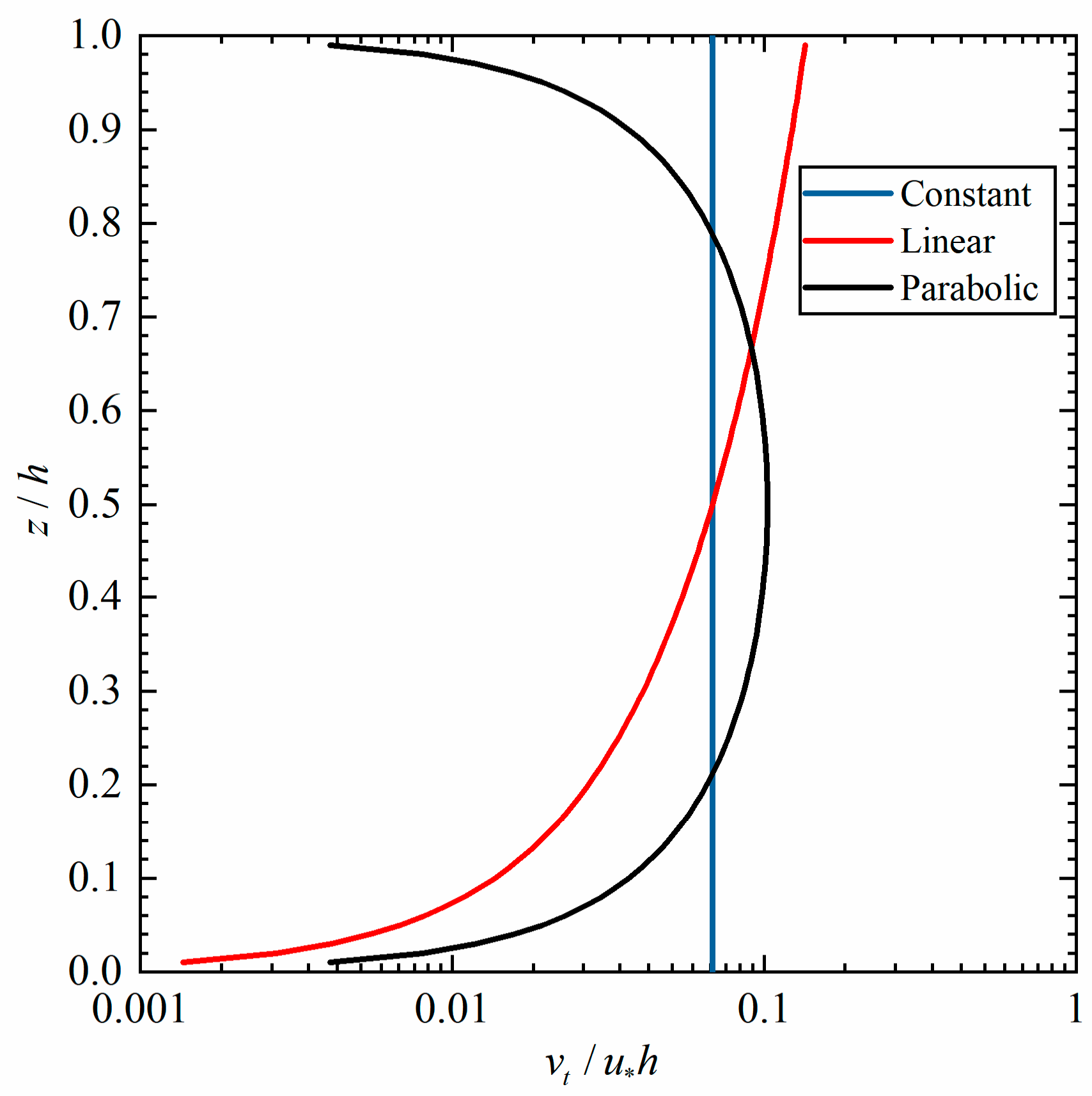
where z denotes the vertical coordinate from the bottom; κ denotes the von Karman constant with a value of 0.41; the values of α 1 and α 2 are 6 and 3, respectively; u denotes the shear velocity; and h represents the water depth. Equations (5)–(7) represent the constant, linear, and parabolic profiles, respectively (Figure 2).
Substituting Equations (2) and (4) into Equation (1) yields the expression below for the sediment transport equation.
D C D t = ω 0 1 C η C z + ξ v t 2 C

2.2. Numerical Algorithm and Discretization

The advection–diffusion equation for suspended sediment concentration is solved explicitly using the values from the previous time step. An adaptive scheme is used to determine the time step size. The time step ranges between t min = 10 5 s and t max = 10 2 s. The Courant number is fixed at 0.1. The solution to the governing equation of sediment transport shall be obtained using the ISPH approach, as used by Ikari and Gotoh [29]. For the convenience of discretization, the first term on the right-hand side of Equation (8) is rewritten as:
ω 0 1 C η C z = ω 0 1 C η C z + C 1 C η z
Its corresponding discretization form is represented as:
ω 0 1 C η C z + C 1 C η z i = ω 0 1 C i η j = 1 N V j C j W i j z + C i j = 1 N V j 1 C j η W i j z
W i j = 7 4 π l 2 1 Q 2 4 2 Q + 1 Q 2 0 Q > 2 ,   Q = r i j l
where W i j denotes the Wendland kernel function; i denotes the target particle and j denotes the neighboring particle; r i j denotes the relative position vector between the target particle i and the neighboring particle j; l denotes the smoothing length.
The second term on the right-hand side of Equation (8) is written in the following discrete form.
ξ v t 2 C i = j = 1 N 8 μ c , i j m j ρ i + ρ j 2 C j C i r i j W i j r i j 2 μ c , i j = 1 2 ξ v t , i ρ i + v t , j ρ j

2.3. Boundary and Initial Conditions

This study follows the solution framework of Hossain et al. [22] for the 2D unsteady sediment transport model by implementing appropriate boundary and initial conditions for the governing equation. Hossain et al. [22] developed a generalized 2D unsteady suspended sediment transport model based on the advection–diffusion equation and solved it numerically using the finite volume method in OpenFOAM. Unlike the Eulerian-based method, which requires specifying a zero sediment flux condition at the free surface, the ISPH model does not. The bottom boundary condition follows Cheng’s [14] generalized formulation, reformulated within the ISPH framework as:
D C D t b o t t o m = z λ C C b o t t o m
where C represents an equilibrium concentration, and when the equilibrium state is reached, the bottom sediment concentration C b o t t o m is equal to the equilibrium concentration C ; λ is the deposition velocity, and is defined as the ratio of deposition flux to bottom sediment concentration, with its value ranging from 0 to ∞. He linked λ to the probability of a bed-level particle that is neither entering suspension nor ceasing its motion. Large values of λ are obtained for particles with large settling velocity, corresponding to a perfectly absorbing bottom bed, whereas a small value of λ corresponds to a reflecting surface, and implies that the sediment particles are prone to be in suspension. In this regard, λ can also be regarded as a reflectivity coefficient of the bottom bed. The subscript ‘bottom’ is positioned at z = a, where a represents the reference height.
At the inlet boundary, an arbitrary concentration profile can be specified as follows:
C x = 0 , z = C x 0 z
where x = 0 denotes the location of the inlet boundary. For the outlet boundary, a zero-gradient condition is adopted.
The initial sediment concentration can be specified as a reasonable value, such as a zero-concentration scenario, denoted as
C t = 0 , x , z = C t 0 x , z
For the convenience of discussion, the governing equation and boundary conditions for suspended sediment transport are normalized by introducing the following dimensionless quantities.
C ^ = C C a ,   t ^ = t u h ,   ω ^ 0 = ω 0 u ,   ν ^ t = ν t u h ,   λ ^ = λ u , x ^ = x h ,   z ^ = z h ,   C ^ = C C a ,   C ^ x 0 = C x 0 C a ,   C ^ t 0 = C t 0 C a ,
where Ca denotes the reference sediment concentration at a given height a, and h denotes the depth of water.
The dimensionless forms of Equations (8) and (13)–(15) can be obtained as follows.
Suspended sediment transport equation:
D C ^ D t ^ = ω ^ 0 1 C a C ^ η C ^ z ^ + ξ v ^ t 2 C ^
Boundary and initial conditions:
D C ^ D t ^ b o t t o m = z ^ λ ^ C ^ C ^ b o t t o m
C ^ x ^ = 0 , z ^ = C ^ x 0 z ^
C ^ t ^ = 0 , x ^ , z ^ = C ^ t 0 x ^ , z ^
Moreover, the dimensionless turbulent eddy viscosity v ^ t in Equation (17) can be calculated according to Equations (5)–(7) and written in a dimensionless form as follows.
ν ^ t ( z ^ ) = κ α 1
ν ^ t ( z ^ ) = κ α 2 z ^
ν ^ t ( z ^ ) = κ z ^ ( 1 z ^ )

3. Model Verification

The generalized non-equilibrium suspended sediment transport model in the present study incorporates Equations (17)–(20). The model will be validated using analytical and semi-analytical solutions for 1D unsteady and 2D steady cases, and using experimental data for 2D unsteady cases.

3.1. Verification of the ISPH Model Against Analytical and Semi-Analytical Solutions

3.1.1. Two-Dimensional Sediment Transport Under Steady Flow with Clear Water Inflow at the Inlet

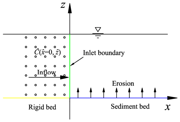
The first example is a 2D sediment transport case under a steady current and is equivalent to the process of suspended sediment transport under a 2D uniform flow, in which clear water flow comes from the upstream inlet and gradually obtains a fully developed boundary layer due to the bottom shear after reaching a flow state. Then, the fully developed clear water flow enters a reach of flume covered with movable sediment particles and starts entraining sediment from the bottom until equilibrium. A schematic of the test case is given in Figure 3. Because the inflow is clear water, the inlet sediment concentration is set to zero ( C ^ x ^ = 0 , z ^ = 0 ). Hjelmfelt and Lenau [11] proposed an analytical model for this scenario by assuming a parabolic distribution of turbulent eddy viscosity. The process involves the development of sediment concentration profiles from the upstream clear water flow towards the downstream equilibrium state and can be described by the following equation, which is derived from Equations (17)–(20).
D C ^ D t ^ = ω ^ 0 C ^ z ^ + z ^ κ z ^ 1 z ^ C ^ z ^
Boundary and initial conditions:
C ^ = 1 z ^ = a ^
C ^ x ^ = 0 , z ^ = 0
Equation (25) is a bottom boundary condition representing the perfect absorption status, which can be derived from Equation (18) by assuming λ ^ = .
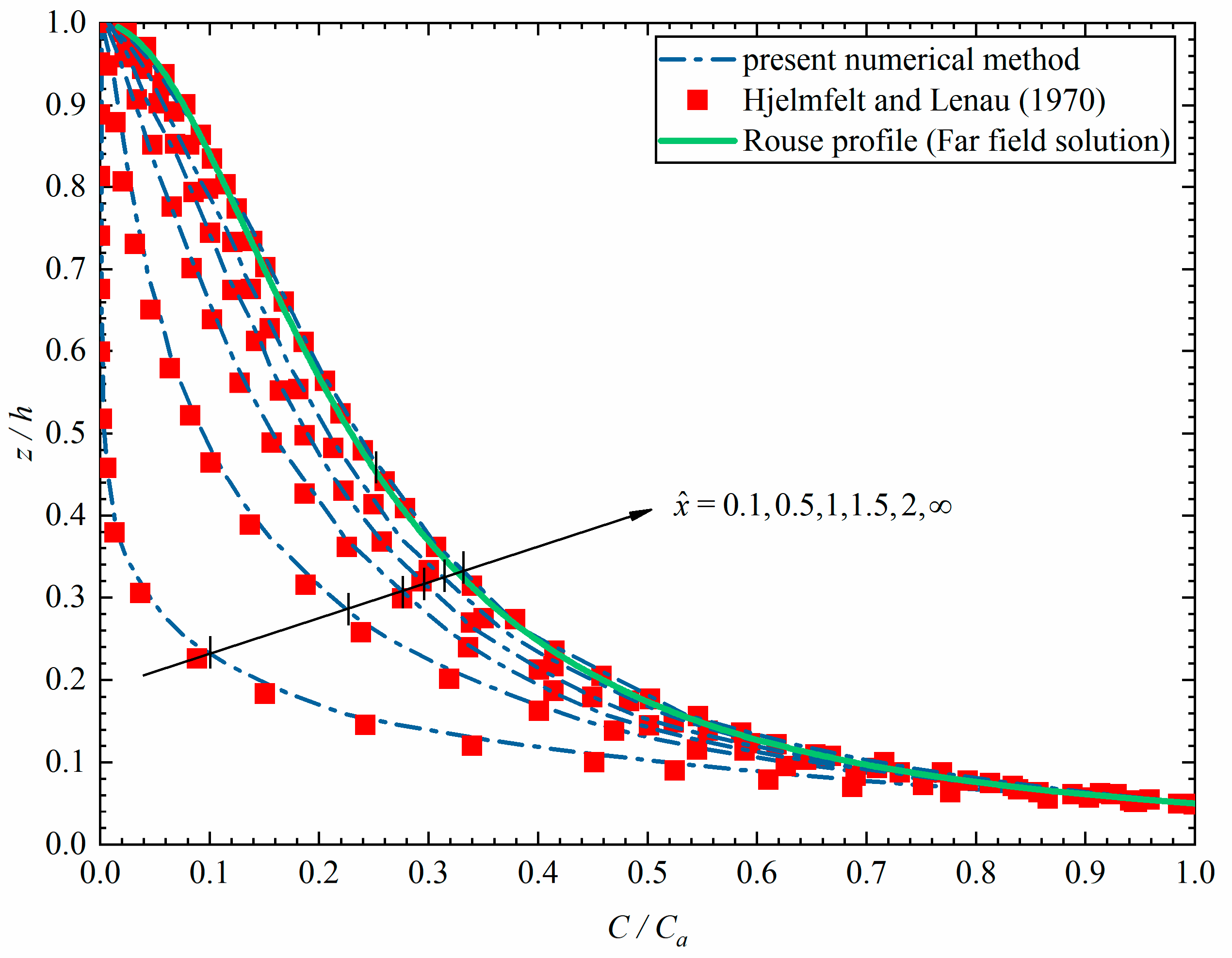
The particle diameter is set as 0.0035 m. The simulation was performed on a 52-core server and took approximately 544 h. The vertical profiles of sediment concentration were acquired at locations x ^ = 0.1 , 0.5 , 1 , 1.5 , 2 , along the flow direction (Figure 4), where the value at x ^ = was actually truncated at x ^ = 100 . From the figure, it can be seen that there is a gradual development of the sediment concentration from a lower level at x ^ = 0.1 all the way down to the Rouse equilibrium solution at x ^ = . Notably, from Figure 4, the results of the numerical simulation agree well with the analytical solution.

3.1.2. One-Dimensional Sediment Transport Under Unsteady Flow with Initial Uniform Sediment Concentration

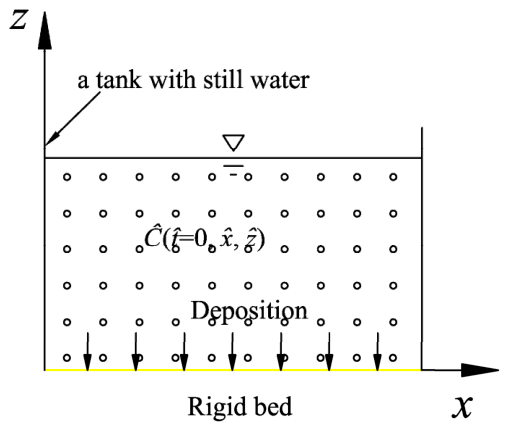
This example describes the settling of sediment in a tank under hydrostatic conditions (mean flow nearly zero), while a vertically constant turbulence is ideally assumed to balance settling and diffusion, following the concept of Cheng [14]. This hydrostatic condition is achieved when a sediment-laden jet enters a tank with standing water and its velocity drops sharply due to the expanded cross-sectional area, forming an initial state close to still water. An equilibrium state is then reached between sediment settling and diffusion. The present study starts the simulation with an initially uniform suspended load concentration C ^ of 1 in a hydrostatic tank and a constant diffusion coefficient for the water. The dimensionless settling velocity ω ^ 0 is set as 1, and the hindered settling effect is tentatively closed. Figure 5 shows a schematic of the test case, in which the initial sediment concentration C ^ t ^ = 0 , x ^ , z ^ is uniformly distributed. Based on Equations (17)–(20), the framework can be readily constructed, as detailed below.
Suspended sediment transport equation:
D C ^ D t ^ = ω ^ 0 C ^ z ^ + α ^ z ^ C ^ z ^
Boundary and initial conditions:
D C ^ D t ^ b o t t o m = z ^ λ ^ C ^ C ^ b o t t o m  
C ^ t ^ = 0 , x ^ , z ^ = 1
where α ^ = ξ κ / α 1 .
The model parameters are listed in Table 1.
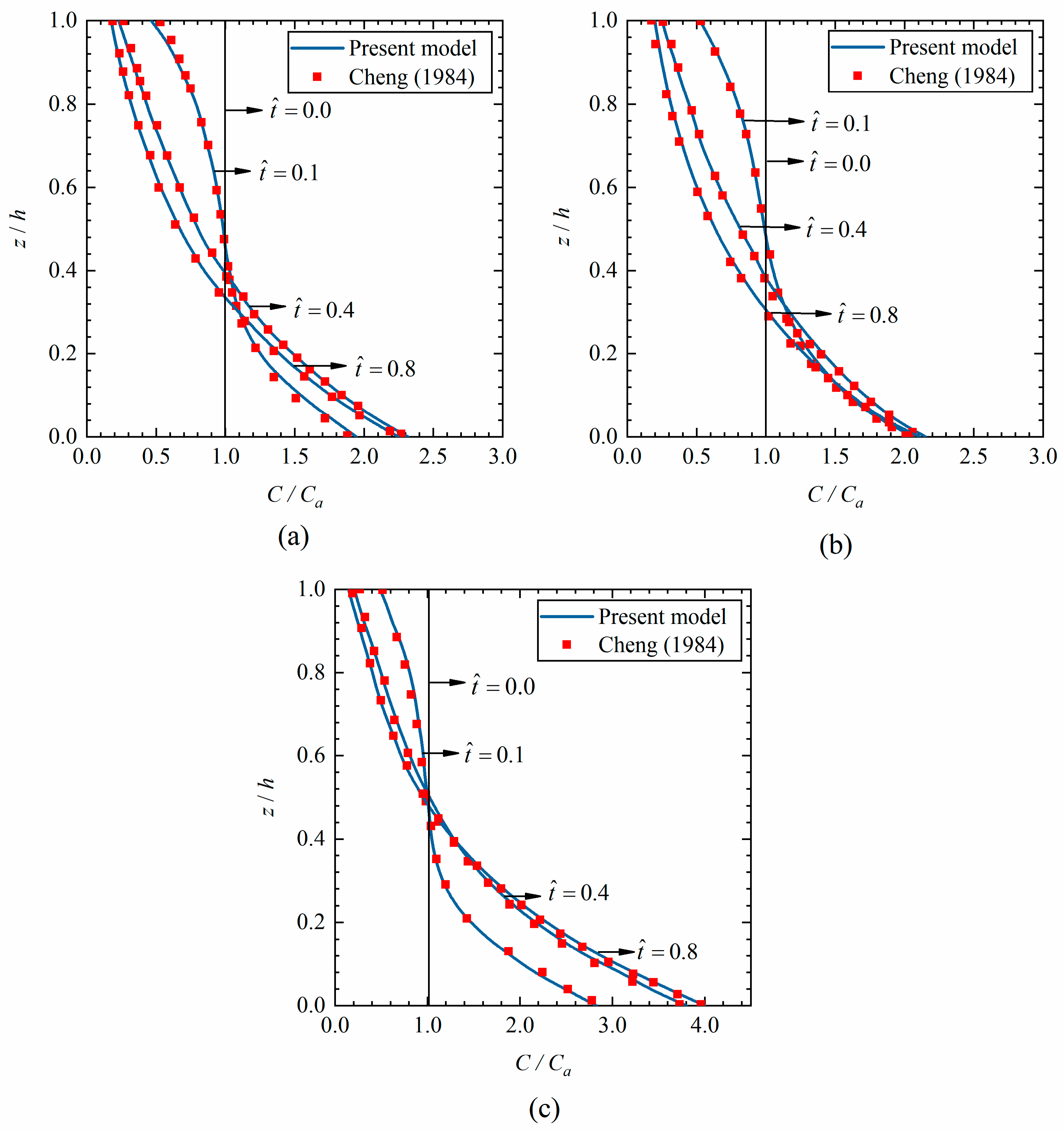
The particle diameter is set as 0.0025 m. The simulation runs for 0.8 s and requires a computational time of about 1 h on a 52-core server. The numerical results of the sediment concentration profiles are provided in Figure 6 for different instants of t ^ = 0.0 , 0.1 , 0.4 ,   and   0.8 . It is seen that the concentration profiles start from a relatively even vertical distribution and gradually evolve to a more uneven profile due to the settling effect. An interesting phenomenon observed in Figure 6a,b is that an overshooting of the sediment concentration occurs at time t ^ = 0.4 , which is signified by the exceedance of the bottom concentration over the equilibrium value C ^ = 2 and then shrinking towards the equilibrium value. In contrast, for Case 3 with a higher equilibrium concentration ( C ^ = 4 ), the overshooting behavior is markedly less pronounced. This overshooting behavior is consistent with the findings of Cheng [14], where the overshoot becomes more pronounced when the deposition coefficient becomes smaller or when the equilibrium concentration is lower. The model results for vertical sediment concentration profiles closely match the analytical solution.

3.1.3. One-Dimensional Sediment Transport Under Unsteady Flow with Initial Arbitrary Sediment Concentration

This case is similar to the case in Section 3.1.2 in that it also describes the deposition process of sediment in a tank with still water, but with an arbitrarily distributed initial sediment concentration and with different eddy viscosity profiles, as in the study by Liu and Nayamatullah [15]. The same schematic shown in Figure 5 is used for this test case. The corresponding expression of the governing equation is as follows.
D C ^ D t ^ = ω ^ 0 C ^ z ^ + z ^ v ^ t C ^ z ^
The boundary and initial conditions are
D C ^ D t ^ b o t t o m = z ^ λ ^ C ^ C ^ b o t t o m
C ^ t ^ = 0 , x ^ , z ^ = C ^ t 0 x ^ , z ^
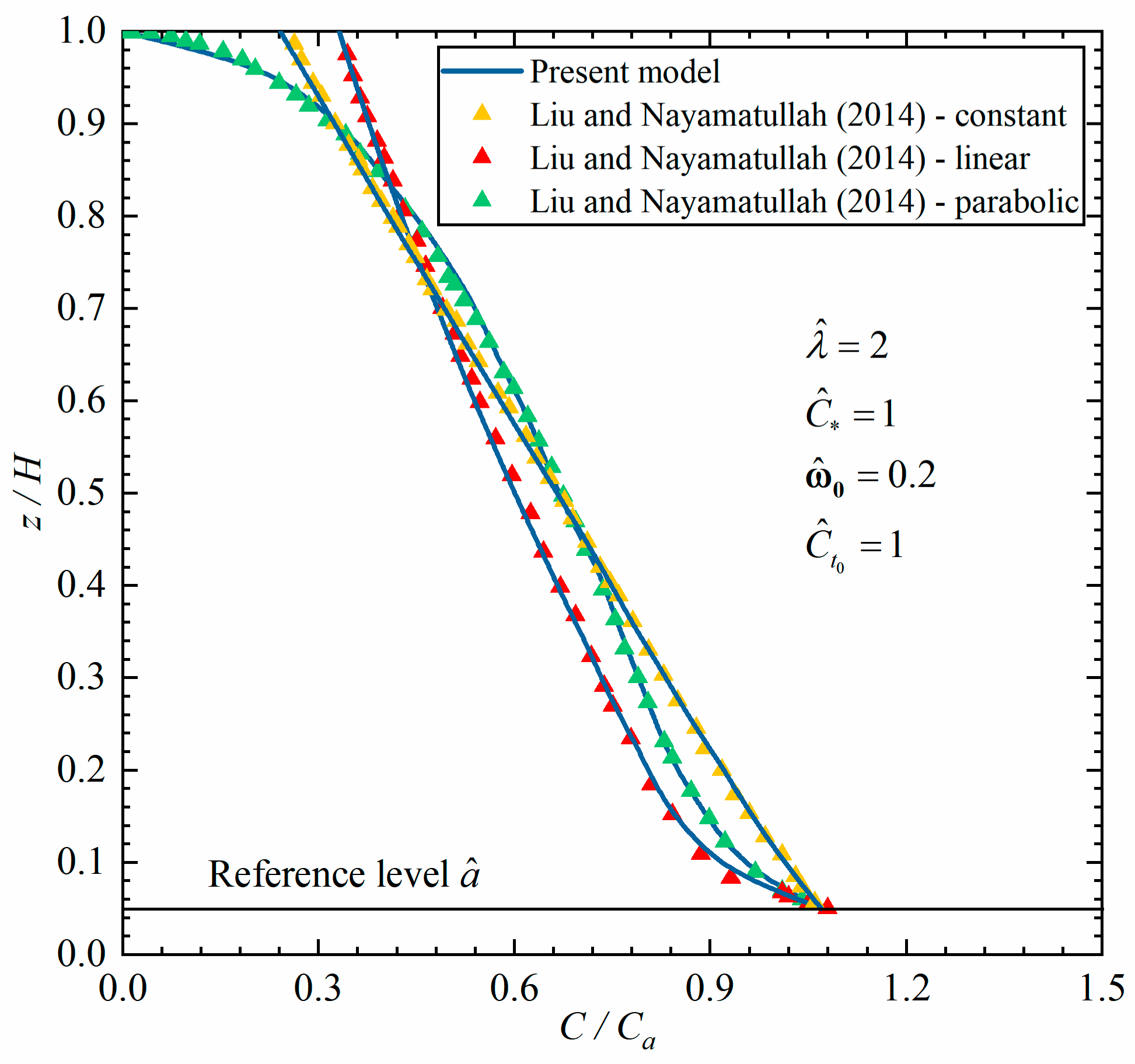
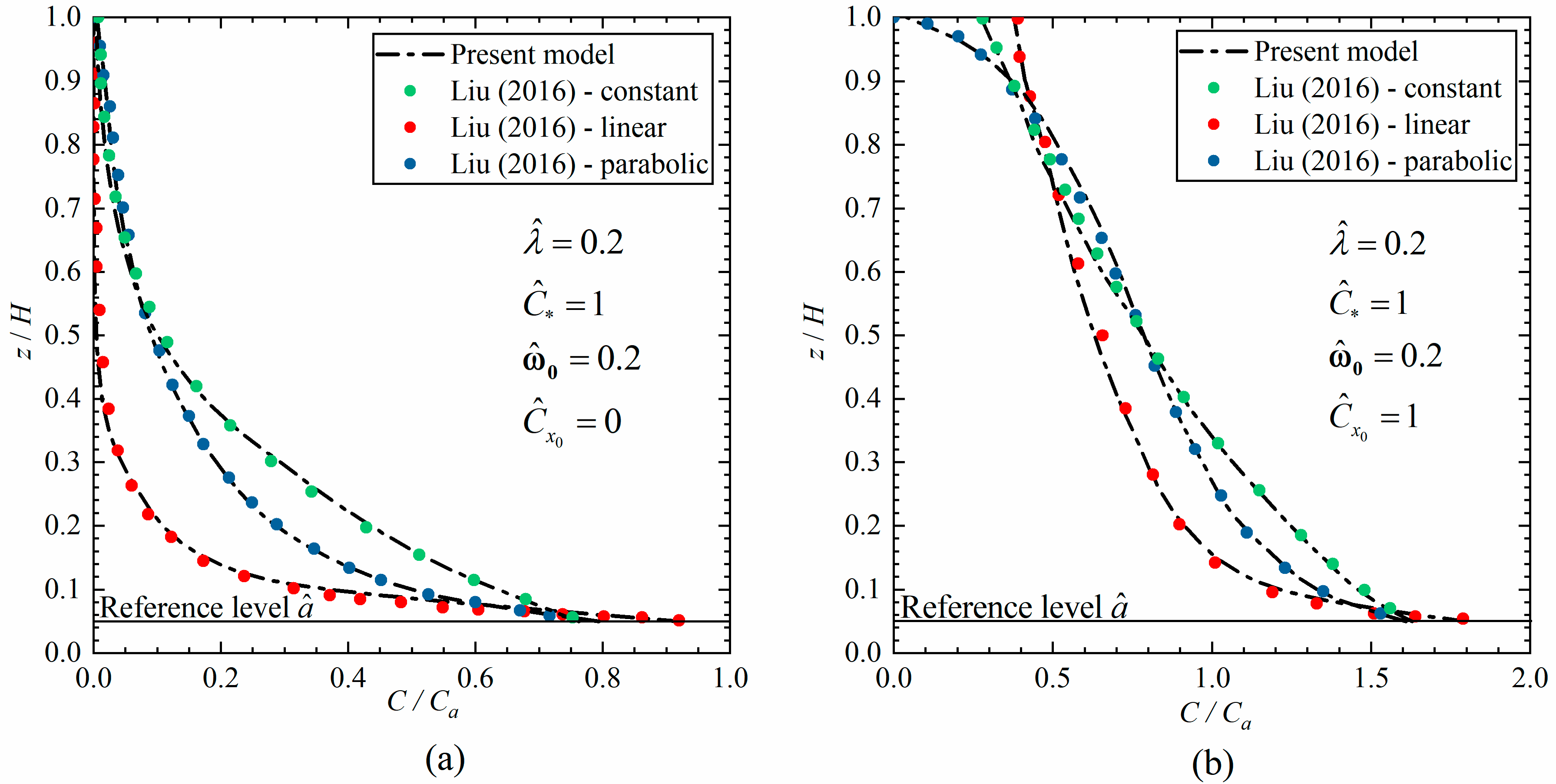
The particle diameter was set as 0.0025 m. The simulation was performed on a 52-core server and took approximately 5 h. Three profiles of eddy viscosity were used in the computation, namely the constant, linear, and parabolic profiles, respectively. Figure 7 shows the results of sediment concentration profiles corresponding to the three eddy viscosity profiles at time t ^ = 2 . It can be seen that the profile of sediment concentration using a constant diffusion coefficient follows a linear vertical profile throughout the water column, whereas the profile of sediment concentration follows a linear variation over most of the water column, except for a small part that deviates from linear around the bottom if using a linearly varying diffusion coefficient profile. The sediment concentration profile deviates almost completely from linear variation if a parabolic profile is used for the diffusion coefficient, especially as it approaches zero at the free surface. Notably, as shown in Figure 7, the numerical results obtained from the generalized sediment transport model are in close agreement with the semi-analytical solution.

3.1.4. Two-Dimensional Sediment Transport Under Steady Flow with Sediment-Laden Inflow at the Inlet

This case is a 2D sediment transport mode under steady current, and it is similar to the case in Section 3.1.1 but has different inflow boundary conditions. Sediment-laden flow with a fixed concentration profile was imposed at the inlet of the flume that was laid with the same bottom sediment as in Liu [1]. The same schematic shown in Figure 3 was used for this test case. The inlet sediment concentration was non-zero ( C ^ x ^ = 0 , z ^ 0 ). The flow velocity imposed at the inlet boundary followed a logarithmic distribution, and the profile of the diffusion coefficient was imposed with three prespecified profiles, the same as those used in Section 3.1.3. The governing equation for suspended sediment transport is
D C ^ D t ^ = ω ^ 0 C ^ z ^ + z ^ v ^ t C ^ z ^
The boundary and initial conditions are
D C ^ D t ^ b o t t o m = z ^ λ ^ C ^ C ^ b o t t o m
C ^ x ^ = 0 , z ^ = C ^ x 0 z ^
The particle diameter was set as 0.0035 m. The simulation was performed on a 52-core server and took approximately 480 h. Figure 8 shows the results of vertical profiles of sediment concentration for the three turbulent eddy viscosity profiles at x ^ = 2 . Figure 8a shows the results using a clear water inlet as a comparison, in which the suspended sediment in the water column completely originates from the sediment entrained from the bottom and transported upwards due to turbulent diffusion. Figure 8b shows the results using a vertically uniform sediment concentration inlet, in which the suspended sediment in the water column comes from both the inlet and the bottom. The concentration near the bottom (Figure 8b) is also positively correlated with the turbulent diffusion coefficient, but the trend is not as significant as in Figure 8a. It is noted that the magnitudes of sediment concentration deviate from each other among those from the three turbulent diffusion profiles, with the result from the constant profile being the largest, the one from the parabolic profile being intermediate, and the one from the linear profile being the smallest. This highlights the close correlation between the rate of sediment diffusion and the diffusion coefficients. As depicted in Figure 8, the numerical solution exhibits favorable agreement with that of the analytical solution.

3.2. Validation of the ISPH Model Against Experimental Data

This subsection validates the 2D unsteady sediment transport model. Because no direct experimental data are available in the literature, we use an indirect verification approach. When time and streamwise distance are large enough, the 2D unsteady solution may approach the 1D steady solution. We therefore compare our numerical results with the classical 1D steady transport experiments of Einstein and Chien [43] and Coleman [44]. These datasets are common benchmarks in sediment transport studies. The experiments of Einstein and Chien [43] had relatively high sediment concentrations, while those of Coleman [44] focused on low-concentration cases. Both experiments used recirculating flumes, and the flume beds were not covered with sand.
The flume in Einstein and Chien [43] was 12 m long and 310 mm wide, with sediment diameters of 0.274 mm, 0.940 mm, and 1.30 mm. Coleman [44] used a flume that was 15 m long and 356 mm wide, with sand diameters of 0.105 mm, 0.210 mm, and 0.420 mm. In both experiments, sediment was added from the upstream end in multiple steps. After each addition, the system was allowed to run for sufficient time until the concentration profile became steady (i.e., no further change with time), indicating that sediment equilibrium had been reached. Only then was the concentration profile recorded at the downstream measuring section near the outlet. This procedure was repeated with increasing sediment supply until sediment saturation was achieved. Detailed experimental parameters are provided in Table 2.
It is assumed in the numerical simulation that sediment concentration is evenly distributed at the inlet section and enters the flume following a steady flow. A parabolic profile of turbulent eddy viscosity was also assumed in the numerical simulation for both of the experiments. Considering the conditions controlling sediment motion, both horizontal and vertical diffusion were included in the model, and therefore, the following form of governing equation was adopted in both experiments.
Suspended sediment transport equation:
D C ^ D t ^ = ω ^ 0 1 C a C ^ η C ^ z ^ + z ^ κ z ^ ( 1 z ^ ) C ^ z ^
Boundary and initial conditions:
D C ^ D t ^ b o t t o m = z ^ λ ^ C ^ C ^
C ^ x ^ = 0 , t ^ = 0 , z ^ = C ^ x 0 , t 0 z ^
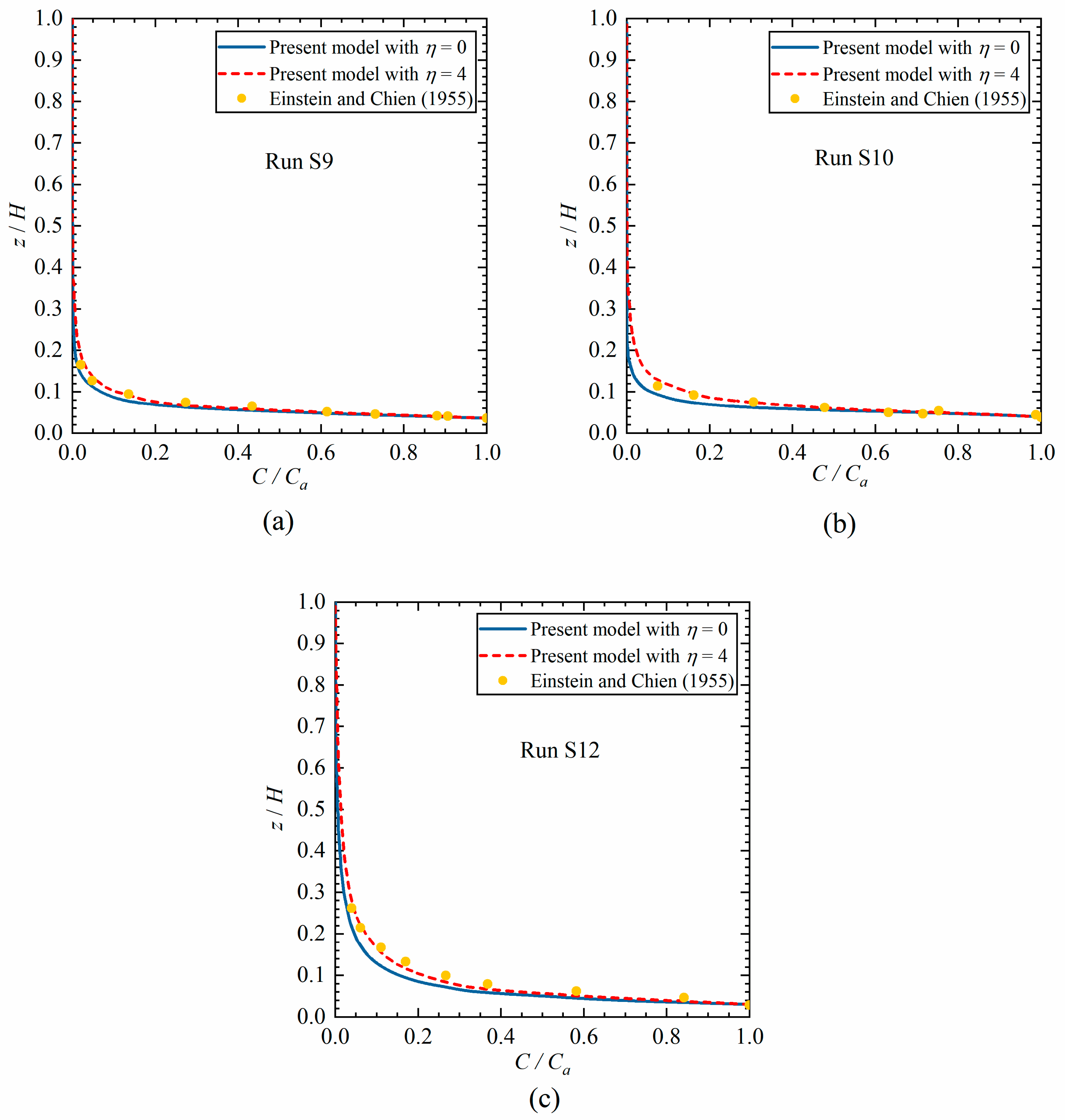
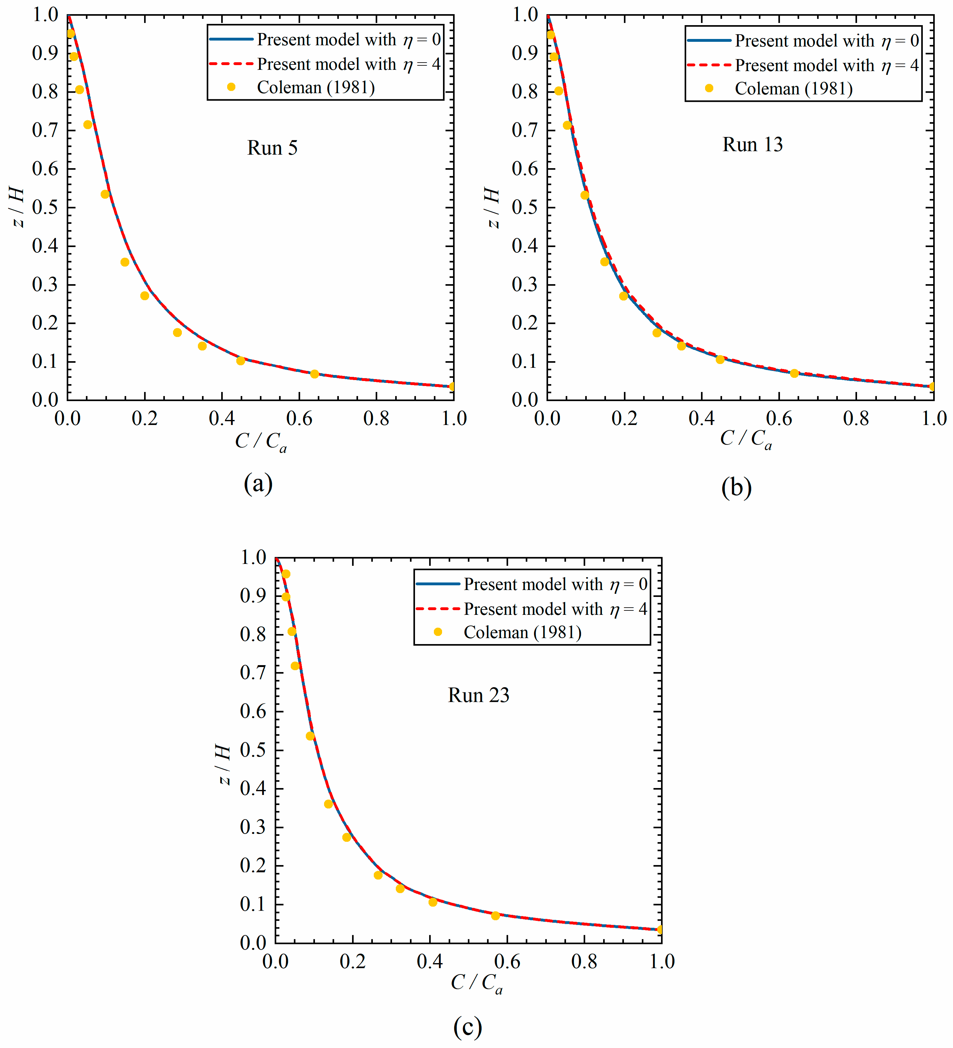
For the simulations corresponding to the experiments of Einstein and Chien [43] and Coleman [44], the particle diameter was set as 0.004 m. The simulations were performed on a 52-core server, taking approximately 720 h for the Einstein and Chien cases and approximately 1000 h for the Coleman cases. Figure 9 and Figure 10 show comparisons of the sediment concentration profiles between the numerical results of the generalized model and the data obtained by Einstein and Chien [43] and Coleman [44], respectively. The relative discrepancy is shown in Table 3 and is calculated using the formula in Equation (39).
PE = 1 N n = 1 N C n e x p C n n u m C n e x p 2
where N denotes the total number of sampling points, and the selection of these sampling points is entirely based on the experiment; C n e x p represents the suspended sediment concentration at the nth sampling point in the experiment; and C n n u m is the sediment concentration at the nth sampling point in the numerical simulation.
Figure 9 and Figure 10 compare the sediment concentration profiles with ( η = 4 ) and without ( η = 0 ) the hindered settling effect. It can be observed that the hindered settling effect increases sediment concentration, and this increase is more evident in the three high-concentration cases from Einstein and Chien [43] than in the three low-concentration cases from Coleman [44]. For Run S10 of Einstein and Chien [43], the relative discrepancy decreased from 3.33% (without hindered settling) to 1.028% (with hindered settling), indicating that a larger η could be considered to further reduce the discrepancy. For the three low-concentration cases from Coleman [44], the data in Table 3 show that accounting for the hindered settling effect has little impact on the relative discrepancy of the simulation results. For example, in Run S12 of Coleman, the relative discrepancy was 0.034% regardless of whether hindered settling was considered, suggesting that the hindered settling effect is negligible for low-concentration cases.

4. Results and Discussion

4.1. Temporal Variation of Concentration Distribution with Different Hindered Settling Effects

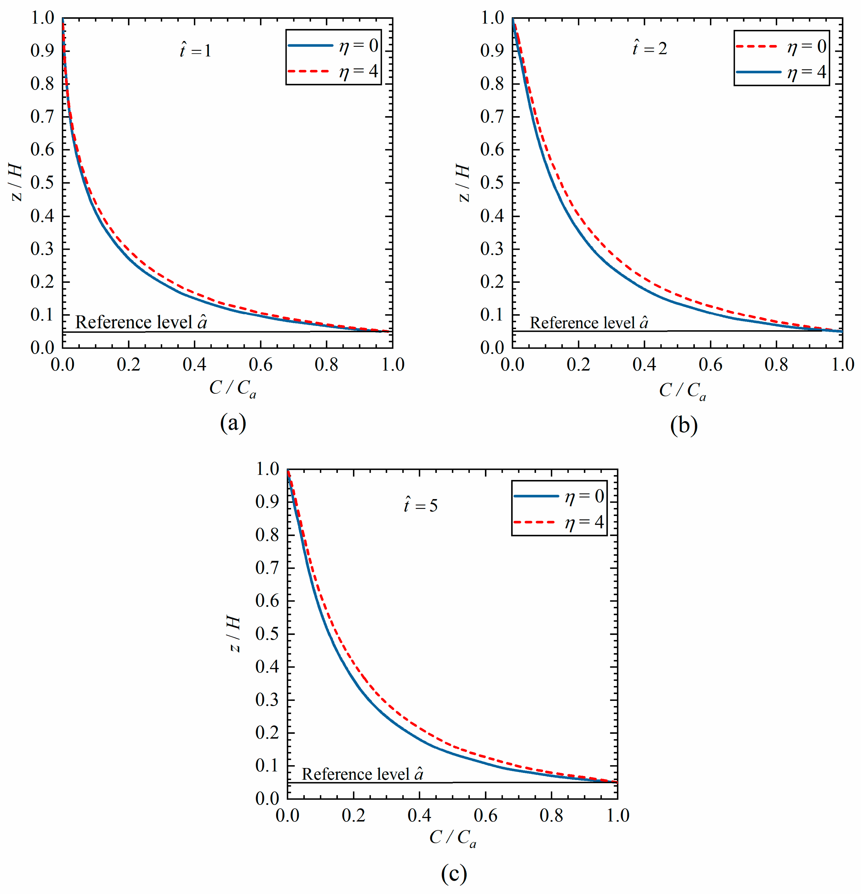
In order to study the temporal variation of sediment concentration distribution affected by the hindered settling effect, a case of 2D sediment transport with steady flow was assumed. Specifically, the case is characterized by a given relatively high reference concentration Ca (taken as 0.07), thus allowing clearer observation of the transient of hindered settling effects on sediment concentration profiles. Furthermore, to prevent interference from excessive sediment sources and simplify the case condition, the inlet was configured as a sediment-free water inflow, and the main flow area was initialized with a zero-sediment concentration. Sediment in the flow was entrained from the flume bottom. A parabolic profile was adopted for the turbulent eddy viscosity. Other parameters are specified in the caption of Figure 11, and are λ ^ = 2 , C ^ =   1 , and ω ^ 0 =   0.2 . A scenario without considering the hindered settling effect was calculated for comparison with η = 0 .
As shown in Figure 11, the hindered settling effect is strongest in the main suspension zone and weaker near the top and bottom boundaries. Near the free surface, the sediment concentration is very low, so particle interactions are negligible. Near the bed, the concentration is high, but the hindered settling effect has already reached its physical limit; the settling velocity is at a minimum, and further increases in concentration do not result in substantial decreases. In addition, the classical Rouse balance (between turbulent upward diffusion and downward settling) dominates the near-bed concentration profile and masks the microscopic hindered settling effect. In the main suspension zone, the concentration is high enough to cause frequent particle interactions but not yet at the limit. As a result, the reduced settling velocity leads to a noticeably higher concentration than in the non-hindered case. Thus, the hindered settling effect is most evident at mid-depth. Over time, the effect becomes increasingly pronounced until the system reaches a steady state.

4.2. Temporal Variation of Concentration Distribution with Different Diffusion Coefficients

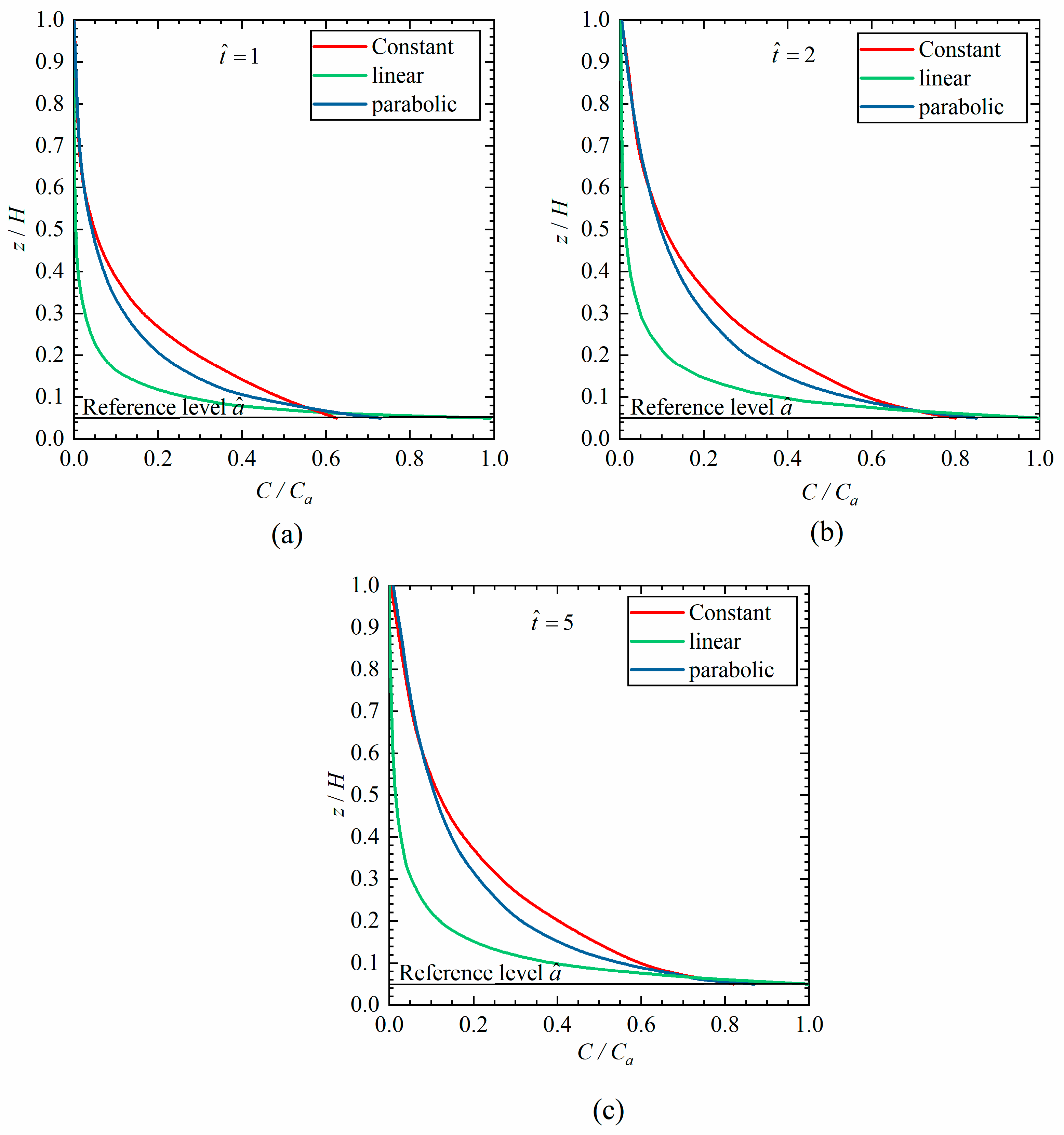
This subsection considers a 2D steady sediment transport process, but with constant, linear, and parabolic profiles for the diffusion coefficient. Also in this example, a clear flow condition is imposed at the inlet. Other parameters are specified in the caption of Figure 12, and are λ ^ = 0 . 2 , C ^ =   1 , η = 4 and ω ^ 0 =   0.2 .
Figure 12 shows the results of sediment profiles obtained with the three different sediment diffusion coefficients at x ^ = 2 for different time instants t ^ = 1 , 2 , 5 . It is evident that different values of diffusion coefficient result in distinct sediment concentration profiles. Generally, a larger diffusion coefficient corresponds to a higher sediment concentration. For example, in the case with a constant diffusion coefficient, the concentration achieves the highest value at the bottom, followed by the parabolic model and then the linear model. Similar results were reported by Liu [1] and Hossain et al. [22]. As time t ^ proceeds, the concentration of sediment with different sediment diffusion coefficient distributions increases and tends towards a stable state.

4.3. Temporal Variation of Concentration Distribution with Different Reference Concentrations

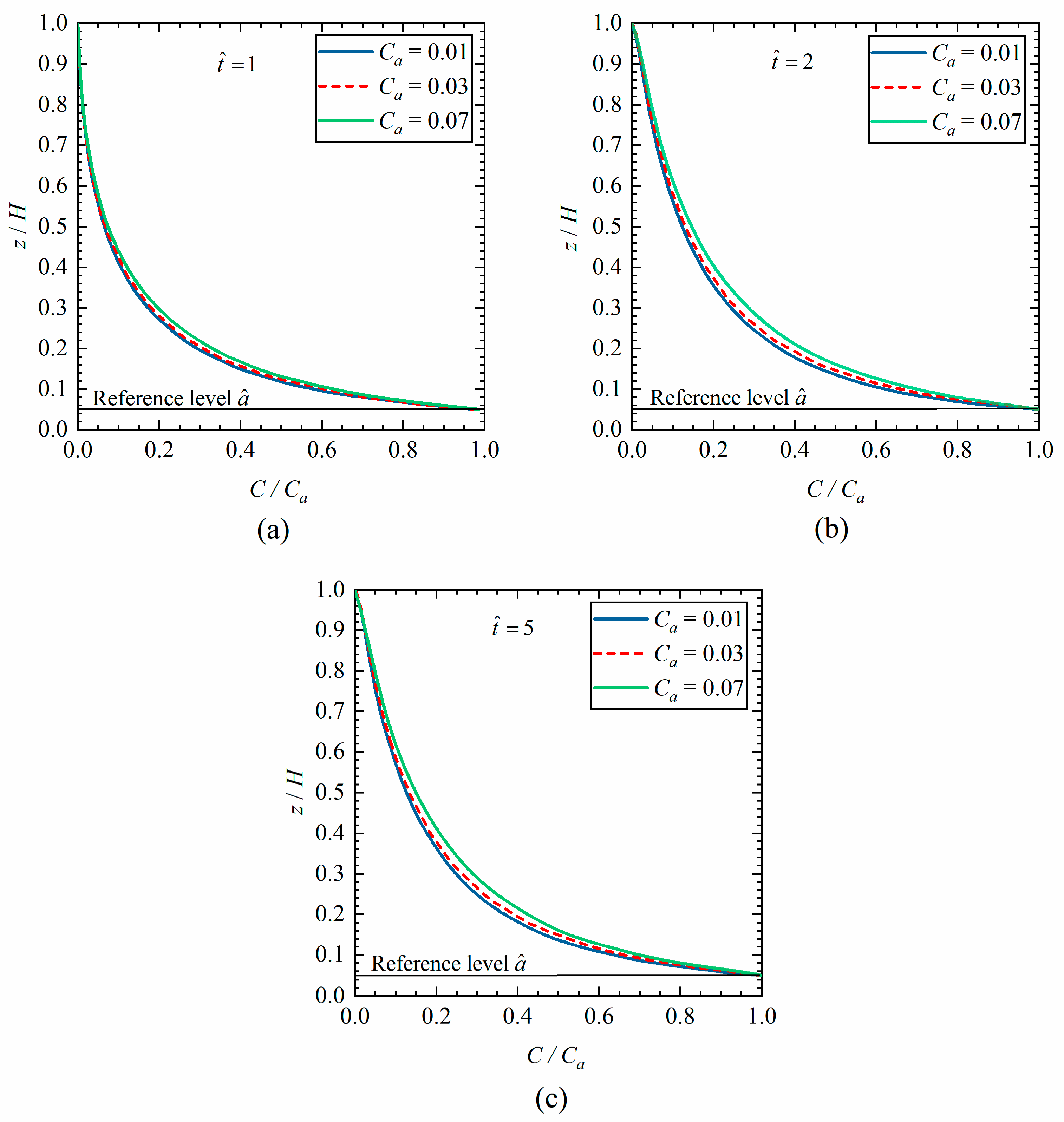
This case demonstrates a 2D steady sediment transport case, as discussed in Section 4.1, but with the main focus on the impact of different bottom reference concentrations. Three bottom reference concentrations were adopted. Similarly, the parabolic model was adopted for the diffusion coefficient; other parameters were set at λ ^ = 2 , C ^ =   1 , η = 4 , and ω ^ 0 =   0.2 , as noted in the caption of Figure 13.
Figure 13 illustrates the impact of the bottom reference concentration on the vertical sediment concentration distribution at different times t ^ = 1 , 2 , 5 , considering the impact of the hindered settling effect. As shown in the figure, the concentration reaches an overall larger value when Ca = 0.07 and a relatively lower value when Ca = 0.01. Moreover, notably from Figure 13, as time progresses, the vertical distribution of sediment concentration, influenced by reference concentration, gradually increases and then stabilizes towards a steady state.

5. Conclusions

We developed a generalized ISPH framework for non-equilibrium suspended sediment transport. The framework includes a generalized bottom boundary condition (GBBC) and accounts for hindered settling and turbulent diffusion. We validated it against analytical and semi-analytical solutions, as well as experimental data.
The main findings of this study are summarized as follows:
(1)
The model reproduces the analytical and semi-analytical results from four test cases: 2D steady flow with clear-water inflow (Hjelmfelt and Lenau [11]); 1D unsteady flow with uniform initial concentration (Cheng [14]); 1D unsteady flow with arbitrary initial concentration (Liu and Nayamatullah [15]); and 2D steady flow with sediment-laden inflow (Liu [1]). The model results agree well with these solutions.
(2)
Using the experimental data of Einstein and Chien [43] and Coleman [44], we validated the model under steady conditions. The hindered settling effect is significant for high-concentration flows (Einstein and Chien) but negligible for low-concentration cases (Coleman). The simulated concentration profiles agree with the measurements.
(3)
The hindered settling effect is most pronounced in the main suspension zone. Near the free surface, the concentration is too low for particle interactions to matter. Near the bed, the effect approaches its physical limit, and the settling velocity drops to a minimum. In the mid-depth region, where particle interactions are frequent, the reduced settling velocity leads to a higher concentration than in the non-hindered case.
(4)
The model varies with different eddy viscosity profiles and with bottom reference concentrations. A larger diffusion coefficient leads to higher sediment concentration, with the constant profile giving the highest bottom concentration. A larger bottom reference concentration also increases the overall concentration. All cases show a rise in concentration with time and reach a steady state.
The present model has two main limitations. First, the turbulence representation relies on simplified eddy viscosity models, which need further validation with more advanced turbulence models for field-scale applications. Second, the reduction exponent of the settling velocity needs further refinement based on more physical experimental data. For future work, we can extend the model to three dimensions by adding suitable sediment boundary conditions on lateral boundaries. We should also include bedload transport, bed deformation, and sediment transport around structures. In addition, more efficient parallel computing strategies are needed to reduce computational cost.

Author Contributions

Conceptualization, S.G. and S.L.; methodology, S.G., S.L. and Y.L.; software, S.G., Y.L. and D.W.; validation, S.G.; formal analysis, S.G.; investigation, S.G., Y.S., D.W. and T.Y.; resources, S.L., Y.L. and Y.S.; data curation, S.G., S.L. and Y.L.; writing—original draft preparation, S.G.; writing—review and editing, S.L., Y.L. and Y.S.; visualization, S.G., D.W. and T.Y.; supervision, S.L.; project administration, S.L.; funding acquisition, S.L. and Y.L. All authors have read and agreed to the published version of the manuscript.

Funding

This research was funded by the National Key R&D Program of China, grant numbers 2022YFC3202400 and 2022YFC3102302, and the National Natural Science Foundation of China, grant number 52201333. The APC was funded by the authors’ institution.

Data Availability Statement

The data presented in this study are available on request from the corresponding author. The data are not publicly available due to privacy and security restrictions.

Conflicts of Interest

The authors declare that they have no known competing financial interests or personal relationships that could have appeared to influence the work reported in this paper.

Nomenclature

Csediment concentration
ω s vertical settling velocity of sediment
v s sediment diffusion coefficient
ω 0 vertical settling velocity of sediment particles in clear water
κvon Karman constant
zvertical coordinate from the bottom
u shear velocity
C b o t t o m bottom sediment concentration
areference height
η reduction exponent of settling velocity
v t turbulence mixing coefficient
ξ inverse of the turbulent Schmidt number
C equilibrium concentration
λ deposition velocity
Careference sediment concentration
z ^ dimensionless vertical coordinate from the bottom
a ^ dimensionless form of reference height
C ^ dimensionless sediment concentration
ω ^ 0 dimensionless vertical settling velocity of sediment particles in clear water
C ^ dimensionless equilibrium concentration
λ ^ dimensionless deposition velocity

Abbreviations

The following abbreviations are used in this manuscript:
2DTwo-dimensional
ISPHIncompressible smoothed particle hydrodynamics
GBBCGeneralized bottom boundary condition
PDEPartial differential equation

References

  1. Liu, X. Analytical solutions for steady two-dimensional suspended sediment transport in channels with arbitrary advection velocity and eddy diffusivity distributions. J. Hydraul. Res. 2016, 54, 389–398. [Google Scholar] [CrossRef]
  2. Rouse, H. Modern conceptions of the mechanics of fluid turbulence. Trans. Am. Soc. Civ. Eng. 1937, 102, 463–505. [Google Scholar] [CrossRef]
  3. Hunt, J.N. The turbulent transport of suspended sediment in open channels. Proc. R. Soc. Lond. Ser. A 1954, 224, 322–335. [Google Scholar] [CrossRef]
  4. Lvan Rijn, C. Sediment transport, Part II: Suspended load transport. J. Hydraul. Eng. 1984, 110, 1613–1641. [Google Scholar] [CrossRef]
  5. Umeyaina, M. Vertical distribution of suspended sediment in uniform open-channel flow. J. Hydraul. Eng. 1992, 118, 936–941. [Google Scholar] [CrossRef]
  6. Chiu, C.-L.; Jin, W.; Chen, Y.-C. Mathematical models of distribution of sediment concentration. J. Hydraul. Eng. 2000, 126, 16–23. [Google Scholar] [CrossRef]
  7. Ghoshal, K.; Kundu, S. Influence of secondary current on vertical concentration distribution in an open channel flow. ISH J. Hydraul. Eng. 2013, 19, 88–96. [Google Scholar] [CrossRef]
  8. Cantero-Chinchilla, F.N.; Castro-Orgaz, O.; Dey, S. Distribution of suspended sediment concentration in wide sediment-laden streams: A novel power-law theory. Sedimentology 2016, 63, 1620–1633. [Google Scholar] [CrossRef]
  9. Kumbhakar, M.; Saha, J.; Ghoshal, K.; Kumar, J.; Singh, V.P. Vertical sediment concentration distribution in high-concentrated flows: An analytical solution using homotopy analysis method. Commun. Theor. Phys. 2018, 70, 367–378. [Google Scholar] [CrossRef]
  10. Mei, C.C. Nonuniform diffusion of suspended sediment. J. Hydraul. Div. 1969, 95, 581–584. [Google Scholar] [CrossRef]
  11. Hjelmfelt, A.T.; Lenau, C.W. Nonequilibrium transport of suspended sediment. J. Hydraul. Div. 1970, 96, 1567–1586. [Google Scholar] [CrossRef]
  12. Sahu, S.N.; Hossain, S.; Sen, S.; Ghoshal, K. Sediment transport in ice-covered channel under non-equilibrium condition. Environ. Earth Sci. 2024, 83, 315. [Google Scholar] [CrossRef]
  13. Sahu, S.N.; Hossain, S.; Gualtieri, C.; Ghoshal, K. Analytical and numerical investigation of suspended sediment concentration profiles in an ice-covered channel using the time-fractional advection–diffusion equation. J. Eng. Mech. 2025, 151, 04025045. [Google Scholar] [CrossRef]
  14. Cheng, K.J. Bottom-boundary condition for nonequilibrium transport of sediment. J. Geophys. Res. Ocean. 1984, 89, 8209–8214. [Google Scholar] [CrossRef]
  15. Liu, X.; Nayamatullah, M. Semianalytical solutions for one-dimensional unsteady nonequilibrium suspended sediment transport in channels with arbitrary eddy viscosity distributions and realistic boundary conditions. J. Hydraul. Eng. 2014, 140, 04014011. [Google Scholar] [CrossRef]
  16. Mohan, S.; Kumbhakar, M.; Ghoshal, K.; Kumar, J. Semi-analytical solution for one-dimensional unsteady sediment transport model in open channel with concentration-dependent settling velocity. Phys. Scr. 2020, 95, 055204. [Google Scholar] [CrossRef]
  17. Ghoshal, K.; Jain, P.; Absi, R. Nonlinear partial differential equation for unsteady vertical distribution of suspended sediments in open channel flows: Effects of hindered settling and concentration-dependent mixing length. J. Eng. Mech. 2022, 148, 04021123. [Google Scholar] [CrossRef]
  18. Kumbhakar, M.; Mohan, S.; Ghoshal, K.; Kumar, J.; Singh, V.P. Semi-analytical solution for nonequilibrium suspended sediment transport in open channels with concentration-dependent settling velocity. J. Hydraul. Eng. 2022, 27, 04021048. [Google Scholar] [CrossRef]
  19. Sen, S.; Kundu, S.; Absi, R.; Ghoshal, K. A model for coupled fluid velocity and suspended sediment concentration in an unsteady stratified turbulent flow through an open channel. J. Eng. Mech. 2023, 149, 04022088. [Google Scholar] [CrossRef]
  20. Woo, H.S.; Julien, P.Y.; Richardson, E.V. Suspension of large concentrations of sands. J. Hydraul. Eng. 1988, 114, 888–898. [Google Scholar] [CrossRef]
  21. You, Z.J. The effect of suspended sediment concentration on the settling velocity of cohesive sediment in quiescent water. Ocean Eng. 2004, 31, 1955–1965. [Google Scholar] [CrossRef]
  22. Hossain, S.; Singh, G.; Dhar, A.; Ghoshal, K. Generalized non-equilibrium suspended sediment transport model with hindered settling effect for open channel flows. J. Hydrol. 2022, 612, 128145. [Google Scholar] [CrossRef]
  23. Luo, M.; Khayyer, A.; Lin, P. Particle methods in ocean and coastal engineering. Appl. Ocean Res. 2021, 114, 102734. [Google Scholar] [CrossRef]
  24. Zhang, C.; Zhu, Y.J.; Wu, D.; Adams, N.A.; Hu, X.Y. Smoothed particle hydrodynamics: Methodology development and recent achievement. J. Hydrodyn. 2022, 34, 767–805. [Google Scholar] [CrossRef]
  25. Khayyer, A.; Violeau, D.; Shao, S.D.; Durante, D. Preface: Latest advances in SPH for fluid mechanics. Eur. J. Mech. B/Fluids 2023, 98, 208–210. [Google Scholar] [CrossRef]
  26. Krištof, P.; Beneš, B.; Křivánek, J.; Št, O. Hydraulic erosion using smoothed particle hydrodynamics. Comput Graph Forum 2009, 28, 219–228. [Google Scholar] [CrossRef]
  27. Ghasemi, V.; Firoozabadi, B.; Mahdinia, M. 2D numerical simulation of density currents using the SPH projection method. Eur. J. Mech. B/Fluids 2013, 38, 38–46. [Google Scholar] [CrossRef]
  28. Tran-Duc, T.; Phan-Thien, N.; Cheong, K.B. A smoothed particle hydrodynamics (SPH) study of sediment dispersion on the seafloor. Phys. Fluids 2017, 29, 083302. [Google Scholar] [CrossRef]
  29. Ikari, H.; Gotoh, H. Numerical modeling of density currents using an Incompressible Smoothed Particle Hydrodynamics method. Comput. Fluids 2018, 167, 372–383. [Google Scholar] [CrossRef]
  30. Tonkin, S.; Yeh, H.; Kato, F.; Sato, S. Tsunami scour around a cylinder. J. Fluid Mech. 2003, 496, 165–192. [Google Scholar] [CrossRef]
  31. Larsen, B.E.; Fuhrman, D.R.; Baykal, C.; Sumer, B.M. Tsunami-induced scour around monopile foundations. Coast. Eng. 2017, 129, 36–49. [Google Scholar] [CrossRef]
  32. Hu, Z.; Qi, W.G.; Li, Y.P. The role of dynamic seepage response in sediment transport and tsunami-induced scour. J. Geophys. Res. Ocean. 2025, 130, e2024JC021084. [Google Scholar] [CrossRef]
  33. Hu, Z.; Li, Y.P. Full-scale tsunami-induced scour around a circular pile with three-dimensional seepage. Coast. Eng. 2025, 197, 104676. [Google Scholar] [CrossRef]
  34. Khayyer, A.; Gotoh, H.; Shao, S.D. Corrected Incompressible SPH method for accurate water-surface tracking in breaking waves. Coast. Eng. 2008, 55, 236–250. [Google Scholar] [CrossRef]
  35. Wang, D.; Li, S.W.; Arikawa, T.; Gen, H. ISPH simulation of scour behind seawall due to continuous tsunami overflow. Coast. Eng. J. 2016, 58, 1650014. [Google Scholar] [CrossRef]
  36. Arikawa, T.; Ikeda, T.; Kubota, K. Experimental study on scour behind seawall due to tsunami overflow. J. Jpn. Soc. Civ. Eng. Ser. B 2014, 70, I_926–I_930. (In Japanese) [Google Scholar] [CrossRef]
  37. Richardson, J.F.; Zaki, W.N. Sedimentation and fluidization (PART 1). Trans. Inst. Chem. Eng. 1954, 32, 35–53. [Google Scholar]
  38. van Rijn, L.C. Principles of Sediment Transport in Rivers, Estuaries and Coastal Seas; Aqua Publications: Amsterdam, The Netherlands, 1993. [Google Scholar]
  39. Gualtieri, C.; Angeloudis, A.; Bombardelli, F.; Jha, S.; Stoesser, T. On the Values for the Turbulent Schmidt Number in Environmental Flows. Fluids 2017, 2, 17. [Google Scholar] [CrossRef]
  40. Chauchat, J.; Hurther, D.; Revil-Baudard, T.; Cheng, Z.; Hsu, T.-J. Controversial Turbulent Schmidt Number Value in Particle-Laden Boundary Layer Flows. Phys. Rev. Fluids 2022, 7, 014307. [Google Scholar] [CrossRef]
  41. Absi, R. Suspended Sediments in Environmental Flows: Interpretation of Concentration Profiles Shapes. Hydrology 2023, 10, 5. [Google Scholar] [CrossRef]
  42. van Rijn, L.C. Mathematical modelling of morphological processes in the case of suspended sediment transport. Ph.D. Thesis, Delft Hydraulic Laboratory, Delft, The Netherlands, 1987. Volume 382. [Google Scholar]
  43. Einstein, H.A.; Chien, N. Effects of Heavy Sediment Concentration Near the Bed on Velocity and Sediment Distribution; University of California: Berkeley, CA, USA, 1955. [Google Scholar]
  44. Coleman, N.L. Velocity profiles with suspended sediment. J. Hydraul. Res. 1981, 19, 211–229. [Google Scholar] [CrossRef]
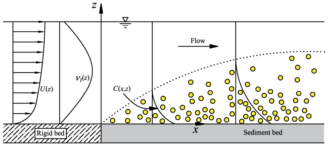
Figure 1. Schematic diagram of non-equilibrium sediment transport [1], where U z denotes the velocity, v t z the eddy viscosity, and C x , z the sediment concentration.
Jmse 14 00900 g001
Figure 2. Eddy viscosity distribution of three empirical formulas.
Jmse 14 00900 g002
Figure 3. Schematic of the 2D sediment transport test case under steady flow.
Jmse 14 00900 g003
Figure 4. Comparisons between numerical results and the analytical solution of Hjelmfelt and Lenau [11] with ς = 0.5 and a ^ = 0.05 (where a ^ is the dimensionless form of reference height with a ^ = a / H ).
Jmse 14 00900 g004
Figure 5. Schematic of the 1D sediment transport test case under unsteady flow.
Jmse 14 00900 g005
Figure 6. Comparisons between numerical results and the analytical solutions of Cheng [14]: (a) case 1, (b) case 2, and (c) case3.
Jmse 14 00900 g006
Figure 7. Comparisons between numerical results and the semi-analytical solution of Liu and Nayamatullah [15]: concentration distribution for three turbulent eddy viscosity profiles at time t ^ = 2 .
Jmse 14 00900 g007
Figure 8. Comparisons of three forms for the vertical concentration distribution at x ^ = 2 between numerical results and the analytical solution of Liu [1]: (a) clear water inlet C ^ x 0 = 0 , (b) uniform sediment inlet C ^ x 0 = 1 .
Jmse 14 00900 g008
Figure 9. Comparisons of the vertical concentration distribution between numerical results and experimental data presented by Einstein and Chien [43]: (a) Run S9, (b) Run S10, and (c) Run S12.
Jmse 14 00900 g009
Figure 10. Comparisons of the vertical concentration distribution numerical results and experimental data presented by Coleman [44]: (a) Run 5, (b) Run 13, and (c) Run 23.
Jmse 14 00900 g010
Figure 11. Comparisons of the vertical concentration distribution at x ^ = 2 and at different times t ^ = 1 , 2 , 5 with different hindered settling effects and λ ^ = 2 , C ^ =   1 , ω ^ 0 =   0.2 , and Ca = 0.07: (a) t ^ = 1 , (b) t ^ = 2 , and (c) t ^ = 5 .
Jmse 14 00900 g011
Figure 12. Comparisons of the concentration distribution at x ^ = 2 and at different times t ^ = 1 , 2 , 5 with different eddy viscosities and λ ^ = 0.2, C ^ =   1 , η = 4 , and ω ^ 0 =   0.2 : (a) t ^ = 1 , (b) t ^ = 2 , and (c) t ^ = 5 .
Jmse 14 00900 g012
Figure 13. Comparisons of the concentration distribution at x ^ = 2 and at different times t ^ = 1 , 2 , 5 with different reference concentrations and λ ^ = 2 , C ^ =   1 , η = 4 , and ω ^ 0 =   0.2 : (a) t ^ = 1 , (b) t ^ = 2 , and (c) t ^ = 5 .
Jmse 14 00900 g013
Table 1. Model parameters.
Case ID λ ^ C ^ ω ^ 0 C ^ t 0 a ^
112110.35
242110.35
314110.35
Table 2. Detailed experimental conditions.
ReferenceRun IDd (mm)h (cm) ω 0 (m/s) u (m/s) a ^ C a
Einstein and Chien [43]S90.94013.620.14100.11800.0360.065
S100.94013.100.10620.12600.0400.099
S120.27413.200.03020.10090.0300.077
Coleman [44]50.10517.10.00660.04100.0350.004
130.10517.10.00660.04100.0350.014
230.21017.00.02080.04100.0350.002
Table 3. The relative discrepancy between experimental and numerical results of sediment concentration.
ReferenceRun ID η = 0 (%) η = 4 (%)
Einstein and Chien [43]S92.4342.050
S103.3301.028
S122.5131.175
Coleman [44]50.2030.206
130.3430.421
230.0340.034
Disclaimer/Publisher’s Note: The statements, opinions and data contained in all publications are solely those of the individual author(s) and contributor(s) and not of MDPI and/or the editor(s). MDPI and/or the editor(s) disclaim responsibility for any injury to people or property resulting from any ideas, methods, instructions or products referred to in the content.