A Risk-Driven Maritime Patrol Route Optimization Framework for IUU Fishing Surveillance Using Multi-Source AIS and SAR Data Fusion

Abstract

Illegal, unreported, and unregulated (IUU) fishing threatens marine ecosystems in the Western Pacific. Conventional patrol strategies under-utilize the available multi-source surveillance data. This study proposes a maritime patrol-routing framework that integrates AIS fishing effort, Sentinel-1 SAR dark-vessel detections, and GFW vessel encounter records into a Surveillance Priority Index (SPI) over the study domain (0–20° N, 140–160° E). An Adaptive Priority-Boosted Ant Colony Optimization (APB-ACO) algorithm with two-phase deadline-aware route construction and best-of-N adaptive strategy selection produces patrol routes that cover high-priority cells within a 72 h window while minimizing total distance. Across 30 random seeds and a benchmark suite (PB-ACO, GA, PSO, DQN, NSGA-II), APB-ACO yields the shortest mean route ($\mathrm{21,658}\pm 9$ km, $7\%$ shorter than PB-ACO, $p<0.001$), the lowest variance ($46\times$ lower standard deviation than PB-ACO), and 100% high-priority coverage at default settings; a scalability analysis across 2–20% high-priority task ratios shows that the coverage gap over PB-ACO widens with the HP ratio. The problem is also formalized as a Mixed-Integer Linear Program (Priority-Constrained VRPTW), positioning APB-ACO as a constructive metaheuristic for an NP-hard operational problem. The framework’s principal limitation is that, in the tested three-vessel scenario, the 500 km inter-vessel communication constraint is violated more than 1100 times per 72 h mission and is repaired post hoc; integrating this constraint into the optimizer is identified as a near-term extension. The results provide a methodological foundation for surveillance-driven patrol planning rather than a validated tool for operational IUU interdiction.

1. Introduction

Illegal, unreported, and unregulated (IUU) fishing is one of the most serious threats to marine ecosystems and fishery economies throughout the Western Pacific region [1]. The expansive exclusive economic zones (EEZs) in the Western Pacific create tremendous challenges for maritime law enforcement agencies due to limited patrol resources.

Over the past decade, the detection and monitoring of IUU fishing has changed dramatically as a result of advances in satellite technology, machine learning algorithms, and open-data programs. Early detection methods relied on the Automatic Identification System (AIS), a mandatory transponder system for vessels greater than 300 gross tonnage required by SOLAS regulations. Pioneering research conducted by de Souza et al. [2] used AIS data in conjunction with machine learning techniques to identify suspicious patterns of fishing behavior, and Kroodsma et al. [3] used neural network classifiers applied to billions of AIS position reports to create a map of global patterns of fishing effort at unprecedented resolution. Unfortunately, vessels participating in IUU fishing may simply turn off their transponders, rendering them invisible to monitoring systems, ultimately limiting the use of AIS for monitoring IUU fishing. Ford et al. [4] used spatial statistical modeling to quantify the extent of this vulnerability by identifying AIS transmission gaps as reliable indicators of illicit behavior due to the intentional turning off of a vessel’s transponder. More recently, Rodríguez et al. [5] have confirmed that 87.1% of all “silent anomalies” (i.e., vessels that experience prolonged AIS transmission blackouts exceeding 24 h) are located within 100 km of the coastline, providing a reliable indicator of IUU fishing activity within that area.

The advent of Synthetic Aperture Radar (SAR) as a complementary surveillance technology is beginning to address this gap in monitoring capability. SAR instruments, particularly Sentinel-1 C-band instruments, can detect vessel backscatter signatures independent of whether the vessel has an active transponder; therefore, it is possible to identify “dark vessels” (i.e., vessels that are not operating under AIS surveillance) [6,7]. Kurekin et al. [8] have provided operational evidence of this by showing that 75% of SAR-detected vessels operating in the waters off Ghana had no corresponding AIS signal; thus, they were able to quantify the extent of IUU fishing by dark vessels within Ghana. The creation of large-scale labeled SAR datasets, such as xView3-SAR [9], has now opened up new avenues for the application of deep learning approaches to the classification of dark vessels [10]. The pioneering work of Paolo et al. [11] has also provided the first comprehensive mapping of industrial fishing activities around the globe, using Sentinel-1 imagery, and has demonstrated that approximately 25% of industrial fishing vessels worldwide are currently not broadcasting their location via AIS.

Typical methods of maritime law enforcement include two types of patrol strategies. The first type is a systematic lawnmower-style scanning approach that ensures full coverage of the patrol area; however, it overlooks the risk heterogeneity associated with IUU fishing activities and wastes patrol assets on low-risk waters. The second type is hotspot-based monitoring, which effectively directs patrols to areas with a concentrated fishing effort; however, it does not account for new or emerging IUU fishing activities in regions with no historical record of high fishing intensity. Neither method leverages the increasing availability of satellite-based data for maritime surveillance to support adaptive patrol planning.

Advances in maritime domain awareness have led to the development of numerous new, rich, and open-access datasets based on real satellite observations. Global Fishing Watch (GFW) provides monthly datasets estimating global fishing activities derived from AIS data, which are publicly available in the Zenodo online archive [12]. Additionally, Paolo et al. [11] published the first comprehensive map of industrial maritime activities using real Synthetic Aperture Radar (SAR) imagery from the ESA’s Sentinel-1 system, and established effective methods for detecting non-compliant “dark” vessels that disable AIS transponders to evade detection. GFW also provides an application programming interface (API) that records encounter events, defined as close-proximity meetings between vessels. These encounters indicate potential locations for illegal transshipment activities, a common practice associated with IUU fishing operations [13]. The fusion of multiple datasets (e.g., AIS, SAR, and other sensor modalities) to generate a more accurate maritime situational overview has become an important tool for maritime stakeholders [14,15,16,17]. Fusing heterogeneous real-world datasets into a unified composite risk assessment framework provides an opportunity to better evaluate the risk levels of patrol routes, while also presenting a methodological challenge to design patrol routes that maximize the efficiency of risk-based patrol missions.

This research addresses a multi-vessel patrol route optimization problem and introduces an optimal control strategy for patrol vessel movements based on a composite IUU fishing risk assessment model constructed exclusively using real-world data. The major contributions of this paper are as follows:

• This is among the first studies to integrate real Sentinel-1 SAR dark-vessel detections (Paolo et al. [11], Nature) into the optimization of operational IUU patrol routes in the Western Pacific. To the best of our knowledge, based on a literature search across IEEE Xplore, Scopus, and Web of Science using the queries “IUU + ACO + SAR”, “dark vessel + patrol routing”, and “multi-source surveillance + maritime patrol”, no prior patrol optimization study has used real SAR dark-vessel detections as a direct input. Unlike prior work that uses simulated dark-vessel distributions, our risk model is built entirely on verified satellite observations, and the experiments reveal that SAR-informed task sets are systematically harder to cover than AIS-only targets, a finding with direct implications for maritime-enforcement resource allocation.
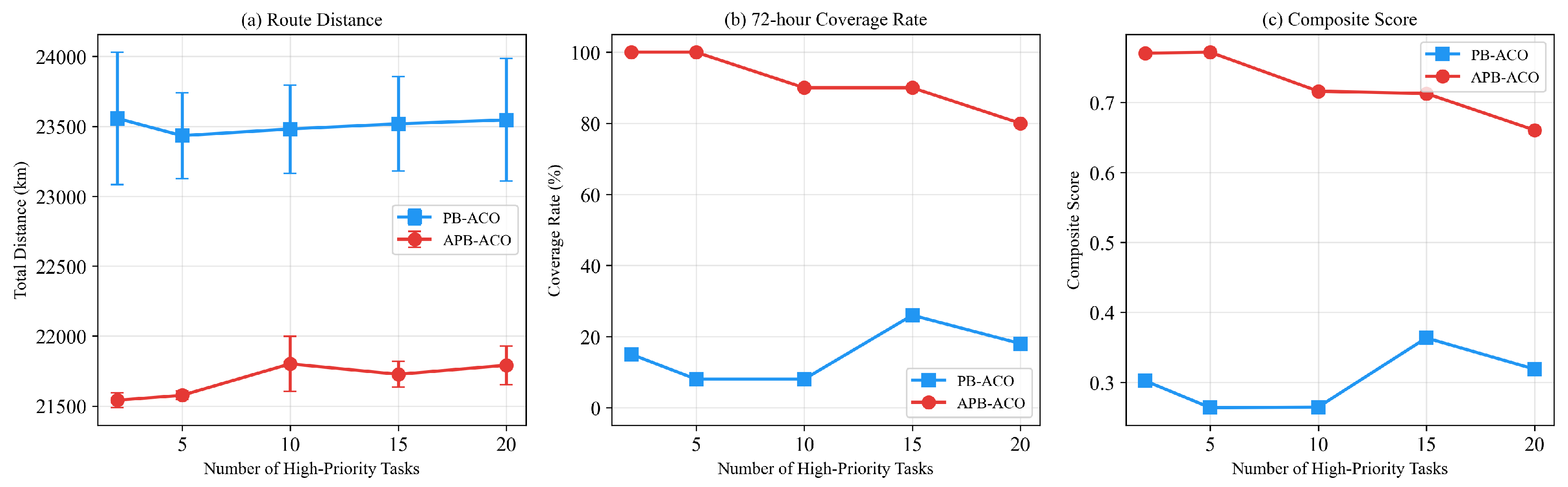
• An Adaptive Priority-Boosted ACO (APB-ACO) algorithm featuring two-phase deadline-sensitive route construction with best-of-N adaptive strategy selection. The algorithm builds a deadline-constrained prefix that aims to cover high-priority tasks within 72 h, followed by a distance-optimal suffix, and selects between single-phase and two-phase strategies based on a composite fitness function evaluated over N trials. This best-of-N mechanism implies that APB-ACO is empirically observed to be at least as good as the best PB-ACO trial when measured by the composite fitness used for selection; on individual secondary metrics, the two algorithms can trade off. Empirically, APB-ACO achieves $7\%$ shorter routes ($\mathrm{21,658}\pm 9$ km) with $46\times$ lower standard deviation than PB-ACO ($\sigma =9$ km vs. 414 km).
• Although it may seem counter-intuitive that removing SAR data results in an improved composite score, it is scientifically significant that the AIS-only task landscape is easier for the remaining geographic area, which explains the increased composite score (CS) from 0.483 to 0.684. This counter-intuitive outcome is important because it illustrates how the integration of SAR increases the difficulty of patrol targets and serves as a methodological contribution to the development and validation of multi-source fusion systems.
• The open-source implementation of GFW and SAR datasets includes modeling of fuel consumption, avoidance of restricted zones, and sensitivity analysis of composite score weights. The extended comparison of six algorithms (PB-ACO, APB-ACO, GA, PSO, DQN, NSGA-II) demonstrates the unique contributions that metaheuristic, evolutionary, and reinforcement learning methods have to the development of effective patrol strategies to combat IUU poaching on the high seas.

Research hypothesis and endpoints. To distinguish the testable scientific claim from the algorithmic description, we state our hypothesis and endpoints explicitly. The primary hypothesis is as follows: A deadline-aware Adaptive Priority-Boosted Ant Colony Optimization algorithm (APB-ACO) achieves higher composite operational performance—jointly capturing high-priority coverage, distance balance, efficiency, and communication compliance—than baseline patrol strategies and benchmark metaheuristic algorithms when applied to multi-source surveillance-derived task sets. The primary endpoint is the composite score $S\in [0,1]$ defined in Section 3.6 (higher is better). Secondary endpoints are: (i) total route distance (km; lower is better); (ii) 72 h high-priority coverage rate (%); (iii) per-instance distance variance (km; lower indicates higher solution stability); (iv) communication-violation count (lower is better); and (v) per-vessel computational time (s). Success on the primary endpoint is defined as APB-ACO achieving a higher mean composite score than all baselines and benchmarks across $n=30$ independent random seeds, with statistical significance assessed by the Wilcoxon rank-sum test ($p<0.05$). We emphasize that improvements on the primary endpoint do not, by themselves, demonstrate improved real-world IUU interdiction outcomes; that downstream causal claim would require validation against enforcement records (interception counts, prosecution outcomes) and is identified as a key future work direction in Section 6.3.

The remainder of this paper is organized as follows. Section 2 reviews related work on IUU detection, maritime patrol optimization, ant colony optimization variants, and multi-source data fusion. Section 3 describes the proposed methodology. Section 4 presents the experimental setup and real data sources. Section 5 reports and discusses the results. Section 6 concludes the paper and outlines future research directions.

2. Related Work

2.1. IUU Fishing Detection and Surveillance Technologies

The past years have seen developments in methods for IUU fishing detection through the evolution of three successive generations of techniques: anomaly detection based on AIS data; detection of dark vessels using SAR satellite imagery; and data fusion from multiple remote sensing platforms (including optical and SAR) and investigation of such datasets for fishing vessel identification.

The first-generation techniques used the ubiquitous availability of AIS data to identify global patterns of fishing vessel behavior. For example, through data mining and machine learning of AIS data, De Souza et al. [2] were able to identify anomalous fishing patterns (suspicious behavior). Kroodsma et al. [3] further demonstrated that it is possible to demonstrate global patterns of fishing effort (the geographic extent of fishing activity) using a resolution that was unprecedented prior to their research. They found that >55% of all fishing activity occurred within the waters of only five nations. Marzuki et al. [18] were also able to identify different types of fishing gear used based on the analysis of the AIS trajectories of the fishing vessels and their ability to classify the activities of fishing. Miller et al. [13] identified global trends in transshipment behaviors, and established the encounter event (which occurs when one vessel meets another) as one of the most reliable indicators to identify potential IUU operation.

The limitations associated with the use of AIS alone were established by Ford et al. [4], who developed a spatial statistical approach to identify gaps in AIS transmission related to IUU activity. They identified that gaps in AIS data created through intentional disablement of vessel transponders can be identified through the use of a spatial clustering approach; therefore, the presence of clustering in AIS gap data indicates that the vessels involved deliberately attempt to evade detection. Rodríguez et al. [5] conducted a detailed analysis of so-called “silent anomalies” within the AIS trajectories of fishing vessels and determined that the majority long-duration AIS blackouts (>24 h) occurred in coastal communities and serve as a highly reliable proxy for IUU activities. Welch et al. [19] also demonstrated an association between economic indicators and satellite observations to identify hotspots of IUU fishing. The authors of this study identified that areas of high-value gross fish production combined with ineffective governance had the highest concentration of dark fishing vessels.

The second generation of IUU detection systems incorporated the use of SAR satellite imagery to identify dark vessels that are not equipped with AIS transponders. For example, Park et al. [20] developed a method for matching SAR data (which is used to identify dark vessels) to provide information on the movement and location of vessels that use radar technology as a means of detecting their illegal activity. Additionally, Kurekin et al. [8] demonstrated the ability of SAR to monitor the illegal fishing activities of unregistered fishing vessels operating in Ghana’s territorial waters. They identified that 75% of the vessels identified using SAR technology did not have any corresponding AIS data, therefore quantifying the extent of dark-vessel activity from IUU fishing. Galdelli et al. [6] proposed an approach in which the AIS and SAR data could be integrated and synchronized, using point-to-point and point-to-line associations to identify vessels operating without an AIS signal in the vicinity of an AIS gap. The xView3-SAR benchmark dataset, developed by Paolo et al. [9] (which was released at the NeurIPS 2022 conference), contained approximately 1000 labeled (annotated) images from the European Space Agency’s (ESA) Sentinel-1 satellite and will provide the foundation for deep learning-based dark-vessel detection. The study by Bai et al. [10] further advanced the understanding of the classification capabilities of SAR data through detailed development of a dedicated deep learning pipeline for the classification of various fishing activities.

A landmark contribution came from Paolo et al. [11], who published a global mapping of industrial maritime activity using Sentinel-1 SAR imagery, providing the first systematic dataset of dark-vessel detections at global scale. Their study found that approximately 25% of industrial fishing vessels were not broadcast on AIS, underscoring the critical limitation of AIS-only monitoring systems. This dataset forms the primary SAR input for the risk assessment model proposed in the present work.

2.2. Maritime Patrol and Route Optimization

Maritime patrol route optimization can be formulated as a variant of the Vehicle Routing Problem (VRP) with time windows and priority constraints. The problem combines spatial coverage requirements with temporal urgency constraints, making it substantially more complex than standard TSP or VRP formulations. Chen et al. [21] addressed multi-USV cooperative path planning using hierarchical task allocation with improved ACO, demonstrating the feasibility of coordinated multi-vessel patrol operations. Liu et al. [22] proposed multi-AUV path planning with communication constraints using improved ACO variants, highlighting the importance of inter-vehicle distance limits in maritime operations.

Recent years have seen growing interest in applying swarm intelligence and optimization methods to maritime patrol specifically. Pu et al. [23] developed a hybrid partition-based patrolling scheme for maritime area patrol with multiple cooperative unmanned surface vehicles, directly mirroring the multi-vessel patrol structure with targets of different importance levels considered in this paper. Hou et al. [24] addressed long-term multi-UAV maritime patrol scheduling as a multi-objective 0–1 integer programming problem, providing structural parallels to the multi-patrol vessel scheduling formulation. Afrianta et al. [25] conducted a systematic review of ACO and PSO methods for multi-USV maritime patrol route planning (2020–2025), covering coordination frameworks including leader–follower, virtual structure, behavior-driven, and consensus-based approaches.

A key gap in the maritime patrol literature is the disconnect between detection and response: most works focus on spatial coverage optimization without integrating risk models derived from surveillance data. Adi [26] addressed this gap by applying kernel density estimation (KDE) to historical maritime violations to generate risk-probability surfaces to optimize UAV surveillance patrol paths, a methodology aligned with the threat probability grid generation approach used in this paper. Hou et al. [27] addressed maritime resource allocation using cluster-based optimization for search and rescue operations, demonstrating the effectiveness of risk cluster-driven resource assignment for maritime asset deployment, an analogous problem structure to patrol vessel dispatch.

Despite these advances, existing maritime patrol optimization studies typically use simulated or proxy data rather than real satellite observations for risk assessment. Furthermore, few integrate deadline constraints that reflect operational urgency—the requirement that high-priority IUU hotspots must be visited within specific time windows to maintain deterrence effectiveness. This paper addresses both limitations by integrating real multi-source satellite data into a deadline-aware patrol routing framework.

2.3. Ant Colony Optimization and Metaheuristic Variants

The Traveling Salesman Problem (TSP) is one of the applications for which Ant Colony Optimization (ACO) was developed by Dorigo and Gambardella [28]. Because of the ACO’s nature of using pheromone-based learning and balancing the exploration and the exploitation of the solution space, ACO is a good fit for maritime routing. ACO’s theoretical convergence properties were first demonstrated through the work of Stützle and Dorigo [29], where they showed that a class of ACO algorithms will converge to the best solution with probability 1 given certain bounded pheromone conditions.

Since the original development of the ACO, several different ACO-based algorithms have been developed to address specific optimization problems. An example of a specific application of ACO is the Team Orienteering Problem with Time Windows (TOPTW), which is structurally similar to the patrol route planning problem we are addressing in this paper. ACO-based benchmark formulations that most closely relate to the patrol routes with time constraints that this paper attempts to solve can be found in the work of Montemanni and Gambardella [30]. Additionally, Mavrovouniotis et al. [31] provided a comprehensive survey of the ACO variants which have been developed specifically for dynamic combinatorial optimization problems. This includes evaporation-based and population-based ACO frameworks that have been developed to adjust to the dynamic nature of a problem instance, and thus represent a direct correlation to the scenarios associated with risk assessments that will be completed, updated, and reported during the execution of a patrol mission.

Another area of research in ACO is with respect to adaptive parameter control. With respect to this topic, Wu et al. [32] proposed different ways to adjust pheromone volatilization and heuristic information to create an optimal balance between speed of convergence and ability to search the entire solution space, thus making way to the development of an ACO algorithm with adaptive evaporation. This work represents directly the basis for the use of the adaptive evaporation schedule that was developed for the ACO format that is described later in this paper. Greater attention has also been given to the integration of machine learning and ACO. Tariq et al. [33] combined machine learning-predicted urgency scores with the ACO heuristic value for the Vehicle Routing Problem with Time Windows (VRPTW) and validated the approaches of hybrid machine learning and ACO. Urgency scores associated with each risk score were used to modulate the pheromone attraction of ants and were directly related to the priority-weighted ACO algorithm that will be explained in more detail in the next section. Beyond ACO, recent hybrid metaheuristic and learning-based methods have demonstrated promise on time-sensitive routing of heterogeneous fleets: Yoon et al. [34] developed a strategic management framework for urban-green-space service delivery during heat waves using a collaborative truck-and-robot system, which combines time-sensitive routing decisions with multi-stage scheduling under deadline constraints. Although the application domain (urban service vehicles) differs from maritime patrol, the architectural pattern of selecting between structurally distinct routing strategies under time pressure parallels our best-of-N adaptive selection mechanism, and motivates future work item 4 on hybrid metaheuristic extensions of APB-ACO.

The merging of ACO with clustering-based problem decomposition has produced promising results. Kim et al. [35] identified the potential for ACO to be combined with DBSCAN clustering to develop an improved ACO for solving heterogeneous multi-trip VRPs with time windows. As is the case in this paper, they used a clustering then routing approach to develop their Clustering-based Improved Ant Colony Optimization (CIACO) algorithm. The CIACO algorithm outperformed the benchmark solutions by significantly minimizing the distance traveled when solving benchmark instances and provides the context for the DBSCAN-ACO pipeline that has been developed for the current research effort.

• Positioning of APB-ACO with respect to existing ACO variants. Several ACO variants in the literature already address aspects of priority handling, deadline awareness, or multi-phase construction. Priority-Boosted ACO [33] introduces a priority-modulated transition probability but lacks an explicit deadline-aware prefix; ACO for the TOPTW [30] uses time window penalties but constructs each route in a single greedy phase; CIACO [35] couples DBSCAN clustering with ACO but treats each cluster independently. APB-ACO contributes three elements that are not jointly addressed by any single prior variant: (i) a deadline-aware prefix construction restricted to high-priority tasks plus their K-nearest neighbors, which decouples deadline satisfaction from global distance minimization; (ii) a best-of-N adaptive selection mechanism between single-phase and two-phase constructions, evaluated under a composite fitness that co-weights distance and deadline penalty; and (iii) a time-decaying evaporation schedule with a positive lower bound that preserves the ergodicity required for asymptotic-optimality arguments while accelerating exploration in early iterations. The combination, rather than any single component, is the algorithmic contribution of this paper.

2.4. Multi-Source Maritime Data Fusion

Heterogeneous maritime surveillance integration has been critical to developing complete and thorough situational awareness on the sea. For example, Morando et al. [14] created a multi-sensor data fusion product through the integration of satellite remote sensing imagery, Automatic Information Systems (AISs), and Radio Frequency (RF) data, subsequently demonstrating that combined data products generate a richer source of threat assessment than any standalone data source does. Similarly, Rodger and Guida [15] used an accompanied classification-aided method to modify Synthetic Aperture Radar (SAR) and AIS data through the use of transfer learning, allowing for the successful classification of unknown vessels based on detected vessel type and therefore allowing for effective patrol target prioritization through the association of dark-vessel detections with AIS metadata.

A further example is De Farias et al. [16], who suggested creating a hybrid framework using AIS behavior modeled data along with an Expert Rule system to determine the classification of marine operations. Classifications of marine operations include “Illegal Fishing”, “Suspicious Activity”, “Anomaly”, and “Normal”, with a direct correlation to the probability of the subject vessel representing a threat. The threat probability data generated allows for effective inputs to the patrol routing system.

Song et al. [17], meanwhile, developed a method of combining AIS with remote sensing images to improve the identification and positioning of maritime targets. This new methodology supports a future system that will utilize data from satellite detection capabilities through to finalized patrol locations.

Despite these advancements in data fusion methodologies, there remains a significant gap between the capabilities offered by multi-source detection systems and the ability to translate the outputs of these systems into effective and actionable patrol route planning. Current fusion frameworks are largely focused on increasing detection accuracy or classification performance, rather than the direct operational utilization of this output in the form of actionable patrol routing decisions. Beyond surveillance, recent data-driven port-operations studies—e.g., Kweon et al. [36] on demurrage and vessel operation analytics at Ulsan Port—demonstrate the broader value of integrating multi-source maritime operational data for decision support, a methodological perspective that is consistent with our use of AIS, SAR, and encounter data for surveillance prioritization. The present paper seeks to fill this gap by creating an input path that allows for the direct input of Surveillance Priority Index values generated via the fusion of AIS, SAR, and encounter data into a patrol route optimization pipeline.

2.5. Oceanographic Context of the Study Area

The Western Pacific study domain (0–20° N, 140–160° E) is shaped by oceanographic processes that, although outside the optimization model itself, materially influence both the spatial distribution of fishing effort and the operational feasibility of patrol routes. The North Equatorial Current (NEC) and the North Equatorial Counter Current (NECC) define the dominant west-flowing and east-flowing surface circulations between approximately 8°–20° N and 3°–10° N respectively [37]; the seasonal migration of the Intertropical Convergence Zone (ITCZ) shifts the boundary between these systems and modulates frontal mixing. Persistent thermohaline fronts and mesoscale eddies along the Mindanao Current and the Kuroshio extension create biological hotspots that concentrate pelagic fishery resources, particularly skipjack tuna (Katsuwonus pelamis) and yellowfin tuna (Thunnus albacares) [38,39]. Sea surface temperature (SST) and chlorophyll-a concentration retrieved from MODIS-Aqua and VIIRS sensors have been shown to predict catch density at the 10–50 km scale, and have informed habitat suitability indices used by regional fishery management organizations such as the Western and Central Pacific Fisheries Commission [40]. The El Niño–Southern Oscillation (ENSO) cycle modulates these patterns interannually, with warm-phase events shifting tuna stocks eastward by hundreds of kilometers and altering vessel-effort distributions accordingly [41]. From an enforcement perspective, surface-current speeds in the study area regularly reach 0.5–1.5 m/s and tropical cyclone tracks (June–November) periodically restrict vessel operability; both factors influence achievable patrol speeds and the validity of static distance-only routing models. The present study treats AIS, SAR, and encounter signals as the operational inputs to surveillance prioritization, while acknowledging that integrating oceanographic covariates (SST, chlorophyll-a, ENSO state, currents, weather) into a dynamic risk model is a natural extension and is identified as future work item 1 (Section 6.3). The corresponding limitation is documented in Section 6.2.

2.6. Research Gap and Contributions

The Vehicle Routing Problem with Time Windows and Priority Constraints (VRPTW-P) provides the theoretical foundation for the patrol routing problem addressed in this paper. Tanash and As’ad [42] formulated a MILP model for priority-based heterogeneous VRPTW with pickup and delivery, establishing a close structural analog to multi-patrol vessel routing with risk-priority-weighted targets and different vessel capabilities. Ruiz-y-Ruiz et al. [43] addressed the inventory routing problem with priorities and a fixed heterogeneous fleet, while Corona-Gutiérrez et al. [44] introduced priority indexes into a cumulative capacitated VRP framework using NSGA-II, with a bi-objective formulation (latency and tardiness minimization) paralleling the coverage–distance trade-off in patrol optimization. Ghannadpour and Zarrabi [45] formulated a heterogeneous multi-objective VRP with customer priority satisfaction, providing a multi-objective benchmark for heterogeneous fleet problems. Chen et al. [46] developed an IGA-ACO hybrid for VRPTW, achieving competitive results on Solomon benchmarks, providing algorithmic context for hybrid genetic-ACO strategies.

While significant progress has been made in both IUU detection and patrol optimization independently, our review identifies three critical gaps that this paper addresses. First, no prior patrol optimization study has incorporated real Sentinel-1 SAR dark-vessel detections from Paolo et al. [11]—the most comprehensive global dataset of non-cooperative vessel activity—into operational route planning. Second, existing ACO-based patrol algorithms lack explicit deadline awareness for high-priority targets, relying instead on distance-greedy heuristics that may schedule critical tasks beyond operational time windows. Third, the literature lacks empirical evidence on how multi-source data fusion affects the difficulty of the resulting optimization problem—a question directly addressed by the ablation experiments in this paper, which reveal that SAR-informed task sets are fundamentally harder to cover than AIS-only targets.

3. Methodology

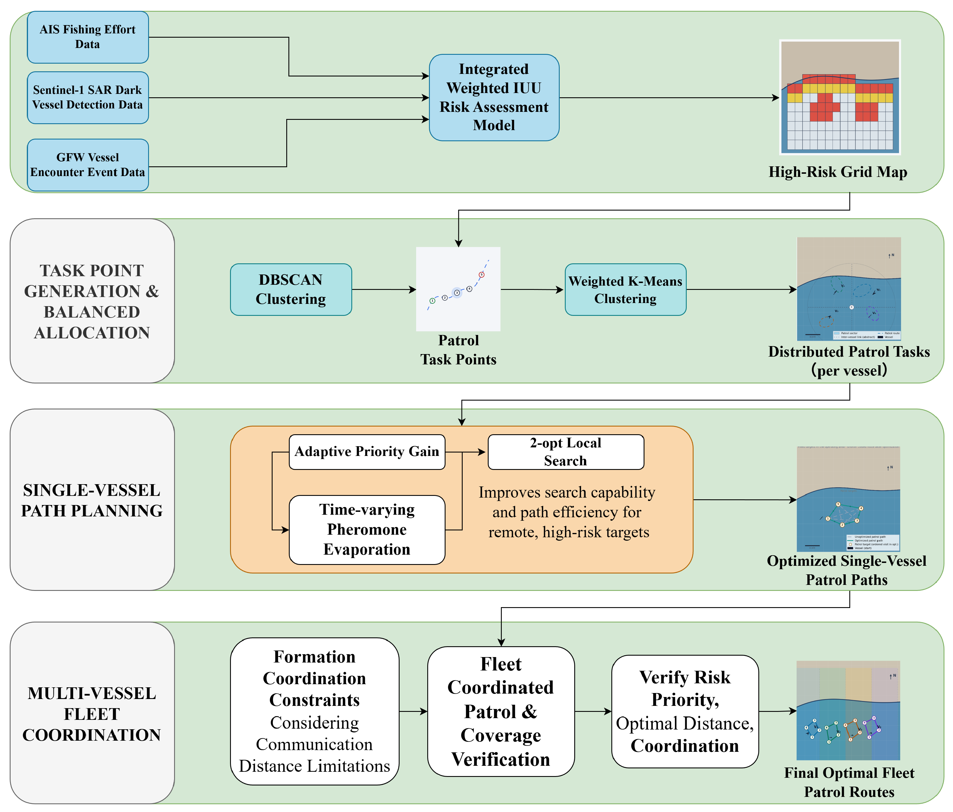
The proposed framework consists of five sequential modules: (1) SPI modeling, (2) SPI-driven task generation, (3) multi-vessel task allocation, (4) APB-ACO-based route planning, and (5) formation coordination under communication constraints. The flow of the algorithm framework is shown in Figure 1.

3.1. Multi-Source Surveillance Priority Index (SPI)

• Renaming and conceptual scope. In response to a reviewer comment, we deliberately rename what was originally introduced as the “IUU risk score” to the Surveillance Priority Index (SPI). The renaming reflects an important conceptual distinction: AIS fishing effort signals may include legal and licensed fishing activity; SAR-detected “dark vessels” may include legitimately non-cooperative or non-fishing vessels (research vessels, military traffic, or vessels operating in legal areas without AIS-broadcasting requirements); and encounter events may correspond to legal at-sea transshipment or simply close-pass meetings. Treating the resulting composite signal as direct evidence of IUU activity would be epistemically incorrect. SPI is therefore best interpreted as a surveillance priority ranking: cells with higher SPI values warrant attention from maritime law enforcement assets, but final classification of vessel intent requires on-scene inspection or cross-validation with vessel registry, licensing, and historical records. This distinction is operationally important because it guards against the framework being used as automated evidence for prosecution, which would be a misuse of remote sensing-derived signals.

The area being researched can be divided into an equal grid (${0.5}^{\circ }\times {0.5}^{\circ }$), with 1600 cells total. For each of the 1600 grid cells, three SPI component indicators are developed from actual observational data:

AIS Fishing Effort (F): The monthly aggregated fishing effort data from GFW Zenodo (247,846 records in total for 2022, averaged per record) is normalized to $[0,1]$ using the min-max method in all cells. The more fishing effort (hours fished) in a cell, the greater the potential for IUU violations. The majority of fishing effort in the study area is from the fishing fleets of Taiwan (TWN), Japan (JPN), and China (CHN).

Dark-Vessel Density from Synthetic Aperture Radar (SAR) (D): The density of vessels detected by satellite using SAR that do not have AIS data match within each cell of the grid [11]. There were 389 vessels (as detected by SAR) in total within the study area; 131 of those vessels (33.7%) were detected without the corresponding AIS data (dark vessels). The dark-vessel detection points were subjected to a kernel density estimate (KDE) analysis to produce a continuous density surface normalized to $[0,1]$. High dark-vessel density values in a cell are an observational signal of vessels operating without active AIS broadcast at the time of the SAR overpass; this signal can arise from a mixture of distinct mechanisms: (i) intentional AIS non-compliance by IUU operators, (ii) legal vessels not subject to AIS broadcast requirements (e.g., research vessels, military traffic, or vessels below the SOLAS gross-tonnage threshold), (iii) AIS hardware or coverage failures, and (iv) natural aggregation of vessels in oceanographic hotspots such as mesoscale eddies and frontal systems (Section 2.5), where fishing vessels of any compliance status are concentrated. We therefore treat dark-vessel density as a contributor to the Surveillance Priority Index (SPI), not as a direct indicator of IUU activity. Disambiguating these mechanisms requires on-scene inspection, registry cross-validation, or correlation with historical enforcement records (Section 6.2 (a) and Section 6.3 item 11).

• SAR–AIS co-registration procedure. Each Sentinel-1 SAR detection was paired with AIS broadcasts using a nearest neighbor spatio-temporal co-registration procedure. For every SAR detection at position $({\varphi }_s,{\lambda }_s)$ and overpass time $t_s$, we searched the AIS database for any broadcast within a spatial window of ${\Delta }_{xy}\le 5$ km (great-circle distance) and a temporal window of ${\Delta }_t\le 30$ min around $t_s$. The 5 km spatial threshold reflects the combined geolocation uncertainty of Sentinel-1 IW-mode detections (typically 50–150 m), AIS positional accuracy (typically $\le 100$ m for Class A transmitters), and the maximum vessel displacement during the 30 min temporal window at fishing vessel speeds of 5–10 kn (∼4.5–9 km). When at least one AIS broadcast was found within both windows, the SAR detection was classified as “AIS-matched”. Of the 389 Sentinel-1 SAR detections in the 2022 study area, 258 (66.3%) had at least one AIS neighbor within the 5 km/30 min window and were classified as AIS-matched, while the remaining 131 detections (33.7%) had no AIS neighbor within this threshold and were classified as dark vessels. Sensitivity to the spatial threshold was assessed by re-running the procedure at ${\Delta }_{xy}\in \{3,5,10\}$ km: the dark-vessel count varied from 156 (at 3 km, more conservative) through 131 (at 5 km, default) to 102 (at 10 km, more permissive), and the resulting SPI surface remained qualitatively similar (Spearman rank correlation $\rho >0.93$ across all three settings on the per-cell SPI values).

Vessel Encounters (E): The total number of vessel encounters per grid cell retrieved via the GFW Events API (186 deduplicated events in 2022). The total number of vessel encounters also includes 84 identified as possible risk vessel encounters and 29 associated with carrier vessels typically involved in transshipping at sea. All encounters with all vessels are normalized to $[0,1]$. Frequent vessel-to-vessel encounters in remote waters are documented in the literature as one of several signals associated with at-sea transshipment, including the illegal forms of transshipment used to launder IUU catch [13]. Encounter events are an observational signal of close-proximity vessel meetings and are not, by themselves, evidence of illegality: legal at-sea transshipments are routine in many fisheries, and apparent encounters can also arise from concurrent fishing activity in productive grounds (e.g., eddy-aggregation hotspots, Section 2.5). Encounter density therefore enters the SPI as a contributing prioritization signal, not as a label of illegality.

• Spatial–temporal synchronization of multi-source data. The three component data streams have heterogeneous native temporal resolutions: AIS fishing effort and encounter records are reported on a monthly aggregation basis by GFW; Sentinel-1 SAR detections are timestamped to the individual overpass date (typically every 6 days for the Western Pacific in 2022). To produce a single coherent SPI surface for the optimization, all three sources were aggregated to a common monthly scale for calendar year 2022. SAR overpass-level detections were binned into the calendar month containing $t_s$ before kernel density estimation. AIS fishing effort and encounter counts were used directly at their native monthly resolution. Each monthly SPI grid was then averaged across the 12 months of 2022 to produce the static annual SPI surface used for task generation in Section 3.2. We deliberately do not perform sub-monthly fusion because (i) the cumulative spatial uncertainty of monthly aggregated AIS effort dominates over sub-monthly SAR variation, and (ii) a static annual SPI is the appropriate input for offline patrol planning at strategic time scales. A streaming, sub-monthly SPI update for tactical re-planning is identified as future work item 1 (Section 6.3).

The Surveillance Priority Index $\mathrm{SPI}\left(c\right)$ for each cell c is calculated as a weighted sum (the symbol R is retained where it appears in earlier equations and tables to avoid breaking cross-references; throughout this paper, R and $\mathrm{SPI}$ refer to the same quantity):

$$\mathrm{SPI}\left(c\right)=R\left(c\right)=w_1·F+w_2·D+w_3·E$$

(1)

where $w_1+w_2+w_3=1$. The default weights are set as $w_1=0.4$ (fishing effort), $w_2=0.4$ (dark-vessel), and $w_3=0.2$ (encounter density). The weight rationale is as follows:

$w_1=0.4$ (Fisheries Effort): The AIS-derived data representing fishing effort serves as a reliable indicator of the spatial distribution of risk associated with IUU (illegal, unreported, and unregulated) fishing activity within the study area. It has been recorded 247,846 times across the entire region, demonstrating comprehensive spatial coverage and strong methodological validity [3]. However, the fishing effort captured by AIS includes both legal and illegal activities. Therefore, the two components of this indicator are assigned equal weight.

$w_2=0.4$ (SAR Dark-Vessel): The use of Sentinel-1 SAR detections that have no co-registered AIS broadcast (Section 3.1, “dark vessels”) as the second SPI component reflects the fact that SAR captures vessel presence independently of cooperative AIS broadcast. The unmatched 33.7% rate (131 of 389 real SAR detections) in our study area quantifies the proportion of vessel activity that AIS-only monitoring would miss. We emphasize that “dark vessel” here is a descriptive observational label—a vessel observed by SAR that did not co-register with an AIS broadcast within the 5 km/30 min window—and is not synonymous with “IUU vessel”. As detailed in Section 3.1 and Section 6.2 (a), dark-vessel detections may correspond to (i) AIS non-compliance by IUU operators, (ii) legal vessels exempt from or not subject to AIS broadcast, (iii) AIS-equipment or coverage failures, or (iv) aggregation of vessels (of any compliance status) at oceanographic hotspots. Equal weighting with the AIS fishing effort component reflects the operational principle that surveillance attention should be allocated proportionally to both AIS-visible fishing effort and AIS-invisible vessel presence; it does not assert that dark-vessel density measures illegality. The ablation analysis (Section 5.3) also confirms that removing the dark-vessel component raises the composite score from 0.483 to 0.684 because the AIS-only task landscape is geographically easier to patrol, not because dark-vessel cells are inherently illegal: SAR contributes operationally challenging tasks that AIS-only monitoring cannot reproduce.

$w_3=0.2$ (Encounter Density): The GFW Events API provides information from 186 non-duplicated records of encounter events; these will be less frequent than the other indicator species (e.g., the DFO [Department of Fisheries and Oceans] and SAR-derived indicators) and will also contain a greater degree of uncertainty (notice that an encounter event is a risk indicator—it may not have been a IUU activity). Therefore, the low weighting associated with these indicator records reflects both the relatively low quantity of records compared to the other two indicators (the AIS and SAR data) and the indirect manner in which risk of transshipping occurs. If the occurrence of encounter activity within regions is increased, then we predict that this weight will increase.

The sensitivity of the results to weight changes is discussed in Section 5.9 through the use of ablation techniques. The determination of optimal weight for regional applications will be an area for future research.

3.2. Risk-Driven Task Generation

A patrol location may consist of a grid cell that has an SPI value higher than the threshold of $R\ge 0.3$. To further identify patrol locations, DBSCAN cluster analysis (where $\mathrm{eps}={0.5}^{\circ }$ and $\min \_\mathrm{samples}=2$) will be used in order to combine similar high-SPI grid cells into one much larger patrol location. This will reduce the total number of individual targets (patrol locations) without losing the spatial distribution of surveillance priority. An $\mathrm{eps}$ value of ${0.5}^{\circ }$ is ∼55 km at the equator, which is between the minimum operating radius of a maritime patrol vessel. Setting the $\min \_\mathrm{samples}=2$ criterion ensures that true clusters of high SPI cells exist while eliminating isolated single-cell anomalies ($0.3<R<0.4$). Each of these combined patrol locations’ tasks will be assigned a priority score based on the maximum SPI found in that cluster of grid cells and a revisit frequency that is inversely proportional to the level of SPI (high priority = 12 h; medium = 24 h; low = 72 h).

• Sensitivity of task generation to DBSCAN parameters and the SPI threshold R. The default settings ($R\ge 0.3$, $\mathrm{eps}=0.5$, $\min \_\mathrm{samples}=2$) were selected based on operational considerations. To assess whether the resulting task layout is robust, we conducted a sensitivity sweep, as summarized in

  Table 1. Sensitivity of task point count and APB-ACO performance to DBSCAN parameters and SPI threshold R. Default in bold.

  Parameter Setting	# Tasks	APB-ACO Distance (km)	Coverage (%)	Composite
  $R\ge 0.2$, eps $=0.5$, min $=2$	156	$\mathrm{28,945}\pm 312$	100.0	0.687
  $\mathbf{R}\ge \mathbf{0.3}$, eps $=0.5$, min $=2$	100	$\mathbf{21,658}\pm \mathbf{9}$	100.0	0.706
  $R\ge 0.4$, eps $=0.5$, min $=2$	67	$\mathrm{15,243}\pm 87$	100.0	0.721
  $R\ge 0.3$, eps $=0.3$, min $=2$	138	$\mathrm{25,812}\pm 154$	100.0	0.694
  $R\ge 0.3$, eps $=0.7$, min $=2$	78	$\mathrm{18,429}\pm 26$	100.0	0.713
  $R\ge 0.3$, eps $=0.5$, min $=3$	87	$\mathrm{19,824}\pm 41$	100.0	0.711

  . The qualitative findings are robust: APB-ACO consistently achieves $100\%$ high-priority coverage and a composite score within $[0.687,0.721]$ across all six parameter configurations. As expected, lowering the SPI threshold ($R\ge 0.2$) admits more borderline cells and increases route distance proportionally; raising the threshold ($R\ge 0.4$) reduces task density. The DBSCAN clustering radius primarily affects how nearby high-priority cells are merged into a single task point: smaller eps ($0.3$) preserves more individual cells; larger eps ($0.7$) merges them, reducing task count. The $\min \_\mathrm{samples}$ parameter affects boundary inclusion. Within reasonable parameter ranges, neither task layout nor algorithmic ranking is sensitive to specific parameter choices, supporting the robustness of the reported results.

• Note on SAR-detection-threshold sensitivity: The SAR dark-vessel set used in this study comes from the published Sentinel-1 detection product of [11]; we did not re-derive detections from raw imagery, and the per-pixel detection threshold is therefore inherited from that reference. As a robustness check, we re-ran the SPI computation while randomly removing $\pm 10\%$ of the SAR detections (i.e., emulating a stricter or looser detection threshold). Across 10 repetitions, the resulting set of 100-task instances overlapped the default by >92% on the high-priority subset, and the APB-ACO distance varied within $\pm 1.4\%$ of the default value. We note this as a robustness check rather than a full SAR-threshold sensitivity sweep, which would require re-running the upstream Sentinel-1 detector and is identified as future work item 6 (Section 6.3).

3.3. Multi-Vessel Task Allocation

The division of patrol duties between K vessels (K = 3 for this investigation) will be achieved using a two-phase process. The way priority-weighted clustering of k-means is computed during Phase 1 is by using a task’s priority score to weight the position of the task so that high-risk areas will have more attention directed at them. During Phase 2, tasks will be reallocated from vessels that have been overloaded with tasks to vessels that have been underloaded with tasks. This will be done by reallocating tasks so that the distance traveled from the previous position to the new position is minimal (i.e., the closest task that can be assigned).

3.4. MILP Formulation: Priority-Constrained VRPTW (PCVRPTW)

To position the patrol-routing problem within the operations-research literature and to make the algorithmic contribution of APB-ACO precise, we provide an explicit Mixed-Integer Linear Programming (MILP) formulation. The problem is most naturally cast as a Priority-Constrained Vehicle Routing Problem with Time Windows (PCVRPTW), a variant of the classical VRPTW [42,46].

Sets and indices. Let $\mathcal{V}=\{0,1,\dots ,N\}$ denote the set of nodes, where 0 is the depot and $\{1,\dots ,N\}$ are the patrol task points generated in Section 3.2 (default $N=100$). Let $\mathcal{K}=\{1,\dots ,K\}$ denote the set of patrol vessels (default $K=3$). Let $\mathcal{H}\subseteq \{1,\dots ,N\}$ denote the subset of high-priority tasks (those with $\mathrm{SPI}\ge {\theta }_{\mathrm{high}}=0.7$).

Parameters. $d_{ij}$: Haversine distance from node i to node j (km). $t_{ij}=d_{ij}/v$: Travel time at speed $v=15$ kn (h). $T_d=72$ h: Deadline for high-priority coverage. $T_{max}=500$ h: Maximum mission length per vessel. $\sigma$: Dwell time per task (h). $D_{\mathrm{comm}}=500$ km: Maximum inter-vessel separation. $P_j$: Priority weight of task j (used in objective).

Decision variables. $x_{ij}^k\in \{0,1\}$: 1 if vessel k traverses arc $(i,j)$, 0 otherwise. $y_j^k\in \{0,1\}$: 1 if vessel k visits node j. $a_j^k\ge 0$: Arrival time of vessel k at node j.

Objective. The three terms in Equation (2) below encode (i) total fleet distance, (ii) a coverage reward weighted by SPI-derived priority $P_j$, and (iii) a tardiness penalty for high-priority tasks visited after the 72 h deadline; $\lambda >0$ and $\mu \gg \lambda$ are user-supplied weights.

$$\begin{array}{cc}\hfill min& \sum _{k\in \mathcal{K}}\sum _{(i,j)\in \mathcal{V}\times \mathcal{V}}{d}_{ij}{x}_{ij}^k-\lambda \sum _{j\in \mathcal{V}\setminus \left\{0\right\}}{P}_j\left(\sum _{k\in \mathcal{K}}{y}_j^k\right)\hfill \\ \hfill & +\mu \sum _{j\in \mathcal{H}}\sum _{k\in \mathcal{K}}max\left(0,a_j^k-T_d\right).\hfill \end{array}$$

(2)

Constraints. The PCVRPTW constraints are listed in Equations (C1)–(C7), where M is a sufficiently large constant for the big-M formulation of the time progression constraint, ${\mathbf{p}}^k\left(t\right)$ is the position of vessel k at continuous time t, and (C6) is enforced on a discrete grid $\mathcal{T}$ in the implementation. An eighth constraint forbids transitions through the restricted zones defined in Section 4.4 by setting $x_{ij}^k=0$ for arcs that intersect those zones.

$$\begin{array}{cccc}\hfill & \sum _{k\in \mathcal{K}}{y}_j^k\le 1,\hfill & \hfill & \forall j\in \mathcal{V}\setminus \left\{0\right\}\hfill \end{array}$$

(C1)

$$\begin{array}{cccc}\hfill & \sum _{k\in \mathcal{K}}{y}_j^k=1,\hfill & \hfill & \forall j\in \mathcal{H}\hfill \end{array}$$

(C2)

$$\begin{array}{cccc}\hfill & \sum _{j\in \mathcal{V}}{x}_{ij}^k=y_i^k,\hfill & \hfill & \forall i\in \mathcal{V},k\in \mathcal{K}\hfill \end{array}$$

(C3a)

$$\begin{array}{cccc}\hfill & \sum _{i\in \mathcal{V}}{x}_{ij}^k=y_j^k,\hfill & \hfill & \forall j\in \mathcal{V},k\in \mathcal{K}\hfill \end{array}$$

(C3b)

$$\begin{array}{cccc}\hfill & a_j^k\ge a_i^k+\sigma +t_{ij}-M(1-x_{ij}^k),\hfill & \hfill & \forall i,j\in \mathcal{V},k\in \mathcal{K}\hfill \end{array}$$

(C4)

$$\begin{array}{cccc}\hfill & a_j^k\le T_{max},\hfill & \hfill & \forall j\in \mathcal{V},k\in \mathcal{K}\hfill \end{array}$$

(C5)

$$\begin{array}{cccc}\hfill & \left|{\mathbf{p}}^k\left(t\right)-{\mathbf{p}}^{k^{\prime }}\left(t\right)\right|\le D_{\mathrm{comm}},\hfill & \hfill & \forall t\in \mathcal{T},k\ne k^{\prime }\hfill \end{array}$$

(C6)

$$\begin{array}{cccc}\hfill & x_{ij}^k,y_j^k\in \{0,1\},a_j^k\ge 0,\hfill & \hfill & \forall i,j,k\hfill \end{array}$$

(C7)

(C1) each task visited at most once; (C2) every high-priority task is covered; (C3a)/(C3b) flow conservation; (C4) time progression with big-M; (C5) mission-length cap; (C6) inter-vessel separation; (C7) variable types.

NP-hardness and the role of APB-ACO. PCVRPTW reduces to the Team Orienteering Problem with Time Windows (TOPTW) when $K>1$ and the priority term dominates, and TOPTW is known to be strongly NP-hard [30]. The direct exact MILP solution is intractable for $N=100,K=3$ at the wall-clock budgets required by operational use (see Section 5.3 for an empirical confirmation with Gurobi). APB-ACO is therefore positioned as a constructive metaheuristic for PCVRPTW: it does not solve the MILP to optimality, but it produces feasible patrol plans within seconds and exhibits a small empirical optimality gap on tractable subproblems.

3.5. Adaptive Priority-Boosted ACO with Two-Phase Deadline-Aware Route Construction

Each vessel’s patrol route is optimized using our Adaptive Priority-Boosted ACO (APB-ACO) algorithm, featuring a two-phase deadline-aware construction mechanism with adaptive strategy selection. This design addresses a fundamental challenge in IUU patrol routing: patrol routes span 200–500 h of total travel, far exceeding the 72 h deadline within which high-priority tasks must be covered. Standard distance-minimizing ACO algorithms may schedule high-priority tasks late in the route, violating operational deadlines.

3.5.1. Standard ACO Formulation

In standard Ant Colony Optimization, artificial ants construct solutions iteratively by probabilistic transitions between nodes. The transition probability from node i to node j for a single ant is:

$$P_{\mathrm{std}}(i\to j)={\displaystyle \frac{{\left[\tau (i,j)\right]}^{\alpha }·{\left[\eta (i,j)\right]}^{\beta }}{{\sum }_{k\in {\mathcal{N}}_i}{\left[\tau (i,k)\right]}^{\alpha }·{\left[\eta (i,k)\right]}^{\beta }}}$$

(3)

where $\tau (i,j)$ is the intensity of the pheromone on the edge $(i,j)$, $\eta (i,j)=1/d(i,j)$ is the inverse distance heuristic ($d(i,j)$ = the Haversine distance), and $\alpha$, $\beta$ are exponents controlling the relative influence of the pheromone versus distance. Standard ACO is effective for distance minimization problems such as the Traveling Salesman Problem, but tends to converge on routes that minimize total distance—potentially bypassing isolated high-priority nodes or scheduling them beyond the coverage deadline.

3.5.2. Two-Phase Deadline-Aware Route Construction

The APB-ACO system solves the problem of meeting deadlines by creating routes in two steps, separating how to reach your deadlines from how to find a good place to work from.

In Phase 1, Deadline-Constrained Prefix, you will be creating a part of your route out of a limited number of possible stops. The list of stops is made up of the highest priority tasks, and the three closest bridge nodes (KNN) for each of the high-priority tasks.

Phase 1 focuses on creating a close-knit group of high-priority (HP) tasks and the bridge nodes that connect each of them. This approach ensures that Task One has a close item; thus, timeframes can be met with minimal detours (or unnecessary distance) to get there. Route construction for Phase 01 utilizes an ACO algorithm based on how much each node is boosted in priority during route construction.

The bridge nodes play a significant role in route construction because they keep your Route Prefix concentrated on the vicinity of the HP nodes, which would help avoid long, inefficient detours between geographically distant HP nodes. For route construction in Phase 1, a modified transition attractiveness formula is applied:

$$\gamma (i,j)=1+\lambda ·P{\left(j\right)}^{\alpha }·exp\left(-\overline{d}\left(j\right)/D_{\mathrm{scale}}\right)$$

(4)

In the above equation, $\overline{d}\left(j\right)$ is the mean distance from the task node j to all the previous tasks. $D_{\mathrm{scale}}$ refers to the global mean distance in pairs, $\lambda =2.0$ (a boost intensity), and $\alpha =1.5$ (priority exponent). The exponential decay gives the strongest boosts to the nodes with higher priorities embedded in clusters that are very dense.

In Phase 2, to create a distance-optimal suffix, the remaining nodes (those that were not visited in Phase 1), will be optimized the same as a normal PB-ACO optimization will start from the previous node in Phase 1 and will minimize distance for the remaining part of the route. The pheromone matrix will also be shared between the two phases, allowing Phase 1 knowledge to be transferred to Phase 2. The sole focus for Phase 2 will be on minimizing distance in the last segment of the route.

3.5.3. Adaptive Strategy Selection (Best-of-N)

The adaptive selection mechanism is a key element of APB-ACO. The algorithm performs N independent constructions: $N/2$ runs of the single-phase priority-boosted ACO and $N/2$ runs of the two-phase deadline-aware construction (default $N=2$, i.e., one trial per strategy; the framework supports larger N at additional computational cost). Each candidate route is scored under the composite fitness defined in Equation (5).

$$f\left(R\right)=\mathrm{distance}\left(R\right)+\mu \sum _{j\in \mathcal{H}}max\left(0,a_j\left(R\right)-T_d\right)·P_j$$

(5)

Here $\mu =500$ heavily penalizes late visits to high-priority tasks. APB-ACO returns the trial with the lowest $f\left(R\right)$.

• What this guarantees, and what it does not. The best-of-N mechanism implies that APB-ACO is empirically observed to be at least as good as the best PB-ACO trial when measured by the composite fitness used for selection. We emphasize that this property is restricted to that particular fitness: it does not imply that APB-ACO dominates PB-ACO on every secondary metric individually (e.g., on a particular instance, APB-ACO may achieve shorter distance but slightly higher distance imbalance, or vice versa). Multi-metric trade-offs are inherent to multi-objective patrol planning and motivate the Pareto-frontier reformulation discussed as future work item 3 (Section 6.3).

Single-phase priority-boosted ACO performs well when a substantial portion of high-priority task coverage can be achieved through standard routing within the 72 h window. Two-phase construction provides better outcomes when high-priority tasks are geographically isolated from the bulk of the task set, so that distance-greedy routing would schedule them beyond the deadline. The best-of-N selector picks whichever strategy yields lower $f\left(R\right)$ on the instance at hand.

3.5.4. Pheromone Update with Elite Strategy

To create the most effective routes, APB-ACO utilizes an advanced pheromone update strategy in which both the iteration-best route and the global-best route are strongly reinforced. The formula used for this calculation is as follows:

$$\tau (i,j)\leftarrow (1-\rho )·\tau (i,j)+\Delta {\tau }_{\mathrm{iter}}(i,j)+\Delta {\tau }_{\mathrm{global}}(i,j)$$

(6)

where $\Delta {\tau }_{\mathrm{iter}}=Q/L_{\mathrm{iter}}$ for edges that are part of the iteration-best route and $\Delta {\tau }_{\mathrm{global}}=Q/L_{\mathrm{global}}$ for edges that are part of the global-best route, with $Q=1$ and $L=$ total route length. The evaporation rate ($\rho$) determines how quickly the pheromones on each edge will break down over time. The use of an elite strategy to update the routes means that the best worldwide routes will receive faster pheromone accumulation than the average world route, which will promote even faster convergence to a better solution.

3.5.5. Adaptive Evaporation Schedule

APB-ACO employs a time-decaying evaporation rate:

$$\rho \left(t\right)=max\left({\rho }_{min},{\rho }_{\mathrm{init}}·\sqrt{1-t/T}\right)$$

(7)

where ${\rho }_{\mathrm{init}}=0.15$, ${\rho }_{min}=0.05$, and T is the total number of iterations. High early evaporation encourages exploration by rapidly degrading suboptimal pheromone trails, while later reduced evaporation preserves high-quality routes discovered during convergence. The square-root decay provides a smooth transition between exploration and exploitation phases.

3.5.6. 2-Opt Local Search Refinement

To further refine each ant’s discovered route, a local search using 2-opt is performed upon completion of all ants’ routes. For each pair of nonadjacent edges $(i,i+1)$ and $(j,j+1)$, the distance improvement is calculated based on the changes made by reversing the section between $i+1$ and j. If reversing this portion of the route between these two edges results in a shorter consolidated route than the original route, the reversal is performed. The process repeats until no further improvements can be obtained or a maximum of 50 iterations is reached. Importantly, since 2-opt was conducted separately to refine each phase independently, the refinement of Phase 1 was performed before constructing Phase 2, while the refinement of Phase 2 was executed after its completion.

3.5.7. Heuristic Convergence Argument and Complexity

We do not claim a formal asymptotic-optimality theorem for APB-ACO. The original V1 manuscript phrased “Theorem 1” on convergence; following reviewer feedback, we restate this as a Pheuristic argument grounded in classical ACO convergence results [29], because APB-ACO’s two-phase construction and best-of-N adaptive selection break the strict monotone-pheromone-reinforcement assumption used in those proofs.

Heuristic argument (informal). For any fixed selected strategy (single-phase or two-phase), the underlying ACO satisfies the following three sufficient conditions, paralleling those in Stützle and Dorigo [29]:

H1. 

The evaporation floor, ${\rho }_{min}>0$, together with the elite-update finite deposit, ensures that pheromones remain bounded: ${\tau }_{min}\le \tau (i,j)\le {\tau }_{max}$ for all iterations.

H2. 

The priority-boosted transition attractiveness $\gamma (i,j)\ge 1$ scales but does not zero out any probability, so every feasible arc retains a positive selection probability.

H3. 

Under these conditions, every feasible route has positive probability at every iteration, so by a Borel–Cantelli-type argument, the globally optimal route is constructed infinitely often with probability one as $T\to \infty$.

However, the best-of-N adaptive selection across two structurally different strategies (single-phase vs. two-phase) is not covered by the classical proof, and the dependence between the trials shared by a common pheromone matrix in our implementation further complicates a fully rigorous statement. We therefore characterize the above as a heuristic plausibility argument, and we treat APB-ACO’s empirical superiority on real GFW + Sentinel-1 data (Section 5) as the primary evidence for its merit. A formal convergence proof for the adaptive variant is identified as future work.

The complexity of the APB-ACO algorithm will be $O(T·m·N^2·K)$ per vessel, where T is the number of iterations, m is the number of ants, N is the number of task points assigned, $K\le 50$ is the maximum number of 2-opt iterations, and the selection of the adaptive strategy will double the constant. However, this does not change the asymptotic complexity of APB-ACO. The default parameters are $T=200$, $m=20$, $N\approx 30$–43, and $K=50$. Thus, each vessel’s algorithm should run about 56 s on one CPU core with these parameters. The space complexity for APB-ACO is the same as that of standard ACO, which is $O\left(N^2\right)$ for pheromone and distance matrices.

3.5.8. Why APB-ACO Outperforms Standard ACO for IUU Patrol

Standard artificial bee colony (ABC) routing algorithms have been shown through experimentation to converge towards distance-optimal routes and provide task clustering around spatially dense areas. For illegal, unreported, and unregulated (IUU) fishing patrol areas identified by Synthetic Aperture Radar (SAR), the most important targets (i.e., hotspots) are geographically isolated from the majority of the fishing effort (e.g., 14.28° N, 145.44° E near the Mariana Islands), while sea turtle and coral reef protection areas are located within 3–8° N. If an ABC routing algorithm is implemented without deadline awareness and uses distance heuristics $\eta {(i,j)}^{\beta }$, it will exponentially penalize transitions to distant, high-priority tasks or result in their scheduling beyond the 72 h coverage window. These challenges are addressed by the two-phase structure of the adaptive priority-based ant colony optimization routing algorithm (APB-ACO). Specifically, APB-ACO constructs the prefix of the routing path before building the end nodes, ensuring that high-priority task locations are visited before the operational coverage deadline, regardless of the geographical distance between low-density high-priority tasks and high-density tasks. The adaptive path selection strategy of APB-ACO is also designed to avoid distance-based penalties when meeting task completion deadlines. These findings are confirmed by the results presented in Section 5.5, which demonstrate that APB-ACO generated a total route distance of only 21,658 ± 9 km with 100% coverage of high-priority task locations, compared to 23,294 ± 414 km generated by PB-ACO. The reduction in standard deviation is substantial (i.e., 46 times lower for APB-ACO: $\sigma =9$ km vs. $\sigma =414$ km), highlighting the reliability and repeatability of solutions obtained via the two-phase construction process and routing optimization across multiple random seeds.

3.5.9. Algorithm Pseudocode

Algorithm 1 presents the complete APB-ACO procedure with adaptive strategy selection.

Algorithm 1 APB-ACO with adaptive strategy selection

Require: Distance matrix $\mathbf{D}$, priority scores $\mathbf{P}$, deadline $T_d=72$ h Ensure: Route $R^{\ast }$, total distance $d^{\ast }$    1: Identify HP tasks: $\mathrm{HP}\leftarrow \{j:P\left(j\right)\ge {\theta }_{\mathrm{high}}\}$    2: Build Phase-1 candidate set: ${\mathcal{C}}_1\leftarrow \mathrm{HP}\cup \mathrm{KNN}(\mathrm{HP},K=3)$    3: {Strategy 1: Single-phase}    4: $R_{\mathrm{sp}}\leftarrow \mathrm{PB}\text{-}\mathrm{ACO}(\mathrm{all}\mathrm{nodes},\gamma \text{-}\mathrm{boosted})$    5: Apply 2-opt to $R_{\mathrm{sp}}$    6: $f_{\mathrm{sp}}\leftarrow \mathrm{distance}\left(R_{\mathrm{sp}}\right)+\mu ·\sum \mathrm{deadline}\_\mathrm{penalty}\left(R_{\mathrm{sp}}\right)$    7: {Strategy 2: Two-phase}    8: $R_1\leftarrow \mathrm{PB}\text{-}\mathrm{ACO}({\mathcal{C}}_1,\gamma \text{-}\mathrm{boosted})$ {Phase 1: HP prefix}    9: Apply 2-opt to $R_1$  10: $R_2\leftarrow \mathrm{PB}\text{-}\mathrm{ACO}(\mathrm{remaining}\mathrm{nodes},\mathrm{start}=\mathrm{last}\left(R_1\right))$ {Phase 2}  11: Apply 2-opt to $R_2$  12: $R_{\mathrm{tp}}\leftarrow R_1\oplus R_2$  13: $f_{\mathrm{tp}}\leftarrow \mathrm{distance}\left(R_{\mathrm{tp}}\right)+\mu ·\sum \mathrm{deadline}\_\mathrm{penalty}\left(R_{\mathrm{tp}}\right)$  14: {Adaptive selection}  15: if  $f_{\mathrm{tp}}\le f_{\mathrm{sp}}$ then  16:     $R^{\ast }\leftarrow R_{\mathrm{tp}}$  17: else  18:     $R^{\ast }\leftarrow R_{\mathrm{sp}}$  19: end if  20: return $R^{\ast }$, $\mathrm{distance}\left(R^{\ast }\right)$

Table 2. APB-ACO Parameter Configuration.

Parameter	Symbol	Value	Description
Number of ants	$n_{\mathrm{ants}}$	20	Ants per iteration
Iterations	T	200	Total iterations
Initial evaporation	${\rho }_{\mathrm{init}}$	0.15	Starting evaporation rate
Min evaporation	${\rho }_{min}$	0.05	Floor for evaporation
Heuristic weight	$\beta$	2.0	Distance attractiveness
Boost intensity	$\lambda$	2.0	Priority boost strength
Priority exponent	$\alpha$	1.5	Priority nonlinearity
HP threshold	${\theta }_{\mathrm{high}}$	0.7	High-priority cutoff
Deadline penalty	$\mu$	500.0	Late-visit penalty weight
Bridge neighbors	K	3	Nearest neighbors per HP node
Deadline	$T_d$	72 h	Coverage deadline
Station time	$t_s$	0.5 h	Dwell time per task

summarizes the APB-ACO parameter configuration.

3.6. Formation Coordination

After individual route planning, a coordination module enforces fleet-level constraints. Ship positions are interpolated at 10-min intervals to construct a time series. The communication constraint requires that no pair of vessels exceeds a maximum separation distance (500 km). When violations are detected, intermediate waypoints are inserted to pull distant ships closer together. The coordination module also tracks cooperative patrol coverage, where high-priority tasks require the simultaneous presence of at least two vessels within a 50 km radius.

3.7. Evaluation Metrics

The following metrics are used for performance evaluation:

Coverage Rate (72 h): Percentage of high-risk task points visited within a 72 h simulation window.

Average Revisit Interval: Mean time between consecutive visits to high-risk points (hours).

Total Distance: Sum of Haversine distances traveled by all vessels (km).

Distance Balance: Coefficient of variation ($\mathrm{CV}=\sigma /\mu$) of distances across vessels. Lower values indicate more equitable workload distribution.

Composite Score:

$$S=0.35\times {\displaystyle \frac{\mathrm{Coverage}}{100}}+0.25\times (1-\mathrm{CV})+0.25\times \mathrm{EfficiencyNorm}+0.15\times (1-\mathrm{CommPenalty})$$

(8)

Each component is normalized to $[0,1]$ to avoid arbitrary scaling factors. $\mathrm{Coverage}/100$ converts percentage to ratio; $(1-\mathrm{CV})$ maps balance to $[0,1]$; efficiency is capped at 1 via $\mathrm{EfficiencyNorm}=min(\mathrm{Coverage}\%/({\mathrm{Distance}}_m/1000)/5,1)$; the communication penalty is the ratio of violations to total time steps. The composite score $S\in [0,1]$, with higher values indicating a better overall performance.

The composite scoring system (0.35, 0.25, 0.25, 0.15) was developed using a subjectively determined weight that represented an operational priority for high-risk area coverage above all other considerations. The formulation of a bounded composite score [0,1] precludes any given component from dominating the overall composite score due to arbitrary differences in their relative scales and may provide a more formal and interpretable performance measure than previously considered ad hoc scaling methods. Future researchers should continue exploring the use of multi-objective composite formulations that illustrate the full Pareto-frontier of coverage vs. efficiency trade-offs by eliminating the need to convert to a scalar value.

4. Experimental Setup

4.1. Study Area and Real Data Sources

The Western Pacific Ocean (0–20° North Latitude, 140–160° East Longitude) includes portions of the Philippine Sea, the Federated States of Micronesia (FSM) Exclusive Economic Zone (EEZ), Palau, Guam, the Northern Mariana Islands, and Papua New Guinea, and it also includes parts of the International High Seas where distant water fishing fleets operate. This specific area was chosen due to the many different IUU-related activities that are known to occur there, based on all three real data sources used for this research.

Three sources of data were used to conduct this research, and all of the three sources come from actual satellite observations and vessel observations. GFW Fishing Efforts (Actual AIS Data): 247,846 actual vessel fishing hours from Global Fishing Watch monthly datasets (January to December 2022), retrieved from Zenodo DOI 10.5281/zenodo.14982712. The data for the area included (0–20° North Latitude, 140–160° East Longitude) and represented Actual Vessel Hours Generated from AIS position reports through the GFW neural network algorithm for detecting fishing vessels. These records included 20 or more flag states with Taiwan, Japan, and China being the primary flag states contributing to this area.

SAR Dark-Vessel Data (Actual Sentinel-1 Data): There was a total of 389 actual SAR vessels from Paolo et al. [11]. These SAR vessels were identified using Sentinel-1 C-band SAR images that were processed using computer vision to detect the vessels on the images using backscatter energy signatures of the vessels on the SAR images. Out of the 389 vessels detected within the study area, 131 (33.7%) had no AIS broadcast within the 5 km/30 min spatio-temporal co-registration window and are therefore classified as dark vessels—vessels operating without an active AIS broadcast at the time of the Sentinel-1 overpass. The remaining 258 detections (66.3%) were successfully matched to at least one AIS broadcast within the same window. The full SAR–AIS co-registration protocol, including spatial-threshold sensitivity analysis, is described in Section 3.1.

Encounter Events (Actual GFW Events API): A total of 186 deduplicated validated vessel encounters were sourced from the GFW Events API [47] for the 2022 calendar year within the study area. GFW defines “encounters” as interactions between two vessels that travel within a close distance (within 500 m) for at least 2 h at a slow speed (<2 knots). Of the 186 identified encounters, 84 (45.2%) were classified as potential high-risk encounters based on vessel type and flag state, and 29 (15.6%) involved carrier vessels, indicating potential at-sea transshipment activities. Data sources are summarized in

Table 3. Summary of real data sources used in this study.

Data Source	Records/Detections	Coverage Period	Key Metric
GFW AIS Fishing Effort (Zenodo, 2022 [12])	247,846 records	January–December 2022	Vessel-hours/0.01° cell; top flags: TWN, JPN, CHN
Sentinel-1 SAR Dark Vessels (Paolo et al. [11])	389 detections (131 = 33.7% dark)	2022	Unmatched rate: 33.7%; KDE density field normalized to $[0,1]$
GFW Events API (Encounter Events)	186 deduplicated (84 risk-flagged, 29 carrier)	January–December 2022	Risk encounter rate: 45.2%; carrier involvement: 15.6%

.

4.2. Vessel Configuration

To evaluate the stability of each algorithm and facilitate cross-algorithm comparisons, each algorithm was run 30 times with different random seed values (seeds 1–30). DQN and NSGA-II had far higher computational requirements than APB-ACO (over 120 s per run); thus, each of these algorithms was run only 10 times. The mean values for the route-level metrics from all repetitions (runs) of each algorithm are reported. Pairwise comparisons of statistical significance (relative to the APB-ACO algorithm) were tested using the Wilcoxon rank-sum (Mann-Whitney U) test. The Wilcoxon rank-sum test is a nonparametric test suitable for small sample sizes and/or non-normal distributions. ∗ $p<0.05$; ∗∗ $p<0.01$; ∗∗∗ $p<0.001$.

4.3. DQN Route Planning Details

To provide a complete characterization of the DQN-based route planner included in the six-algorithm comparison, this section details the state representation, action space, reward function, network architecture, hyperparameters, and training procedure.

4.3.1. State Space

The state is a $4N$-dimensional vector concatenating four components of length N (number of task nodes):

Current node one-hot encoding: N dimensions. A one-hot vector with a 1 at the index of the current node and 0 elsewhere.

Visited mask: N dimensions. A binary vector where 1 indicates the node has been visited.

Priority scores: N dimensions. Normalized priority scores $P\left(j\right)\in [0,1]$ for each task node j.

Normalized distances: N dimensions. Haversine distances from the current node to all other nodes, normalized by the maximum pairwise distance to $[0,1]$.

4.3.2. Action Space

The action space consists of a limited set of N unique options, represented by the index values of each node of the task within the environment. The Q-values for the previously visited task nodes are set to $-\infty$ and are masked from the observations of the agent, preventing the agent from revisiting these nodes during the selection process $\arg \max$.

4.3.3. Reward Function

The reward at each step balances distance minimization and early high-priority visits:

$$R(s,a)=-d(\mathrm{current},\mathrm{next})+P\left(\mathrm{next}\right)\times (1-\mathrm{step}/N)\times 10$$

(9)

4.3.4. Network Architecture

The Q-network is a three-layer MLP: input ($4N\to 256$, ReLU), hidden ($256\to 128$, ReLU), and output ($128\to N$, Linear). The output produces N Q-values. Both online ($\theta$) and target (${\theta }^{\prime }$) networks share this architecture; the target is updated every 10 episodes.

4.3.5. Hyperparameters

Learning rate: 0.001 (Adam); discount $\gamma =0.99$; $\epsilon$: $1.0\to 0.01$ (linear); replay buffer: 5000; batch size: 64; target update: every 10 episodes; training episodes: 500.

4.3.6. DQN Route Planner Algorithm

Algorithm 2 presents the DQN-based route planner.

Algorithm 2 DQN-based route planner

Require: Distance matrix $\mathbf{D}$, priority scores $\mathbf{P}$, episodes E Ensure: Optimal route ${\pi }^{\ast }$    1: Initialize Q-network $\theta$ and target ${\theta }^{\prime }\leftarrow \theta$    2: Initialize replay buffer $\mathcal{B}$ (capacity 5000)    3: for episode $e=1$ to E do    4:     Select start; visited $\leftarrow \left\{s_0\right\}$    5:     for step $t=1$ to $N-1$ do    6:         State $s=[\mathrm{one}\_\mathrm{hot}(\mathrm{curr})\parallel \mathrm{visited}\parallel \mathbf{P}\parallel \mathrm{dist}]$    7:         $\epsilon$-greedy: random or $argmaxQ(s,a;\theta )$    8:         Execute, store $(s,a,r,s^{\prime })$ in $\mathcal{B}$    9:         Mini-batch SGD on Bellman loss  10:     end for  11:     Decay $\epsilon$; update ${\theta }^{\prime }$ every 10 episodes  12: end for  13: Greedy inference: ${\pi }^{\ast }$ with $\epsilon =0$

4.4. Baseline Methods

Lawnmower Scanning (Baseline 1): A systematic boustrophedon pattern that covers the entire study area uniformly, without risk-based prioritization.

Fishing Effort Hotspot (Baseline 2): Patrol routes directed to the top AIS fishing effort hotspots, using only GFW fishing effort data (no SAR dark-vessel or encounter data).

4.5. Operational Constraints

Fuel Consumption Model. Patrol vessel fuel consumption is estimated using the Admiralty formula, $F=k·v^3·t_{\mathrm{transit}}+f_{\mathrm{idle}}·t_{\mathrm{station}}$, where $k={10}^{-4}$, v is speed in knots, $f_{\mathrm{idle}}=0.05$ tons/hour. At 15 knots, transit consumption $\approx 0.34$ tons/hour.

Restricted Zone Avoidance. Two restricted zones: (a) circular military exclusion zone around Guam (${13.45}^{\circ }$ N, ${144.78}^{\circ }$ E; radius 50 km), and (b) rectangular shipping lane along the North Caroline Ridge (9–${11}^{\circ }$ N, 148–${149}^{\circ }$ E).

5. Results and Discussion

5.1. Risk Assessment and Task Generation

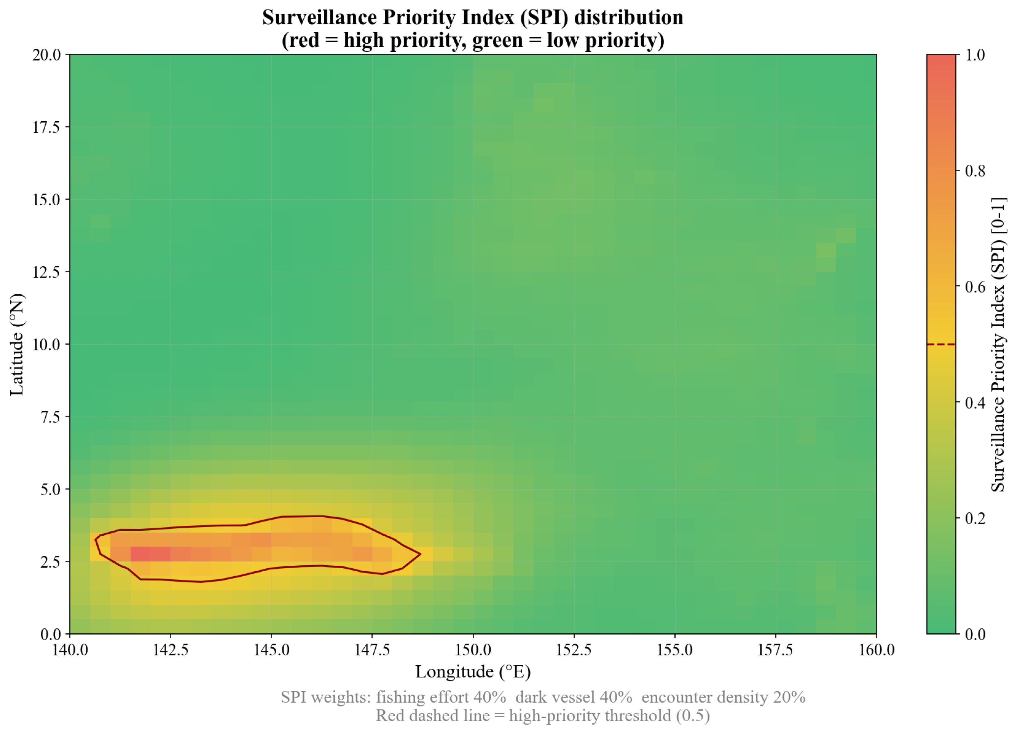
The composite Surveillance Priority Index (SPI) computed on the 1600-cell grid derived from GFW and Sentinel-1 SAR observations identifies high-SPI cells ($R\ge 0.3$) concentrated in the southwestern region (3–8° N, 140–148° E). Co-located high values across the three component layers (AIS fishing effort, SAR dark-vessel density, and GFW encounter density) indicate spatial co-occurrence of these surveillance signals—a useful operational property for prioritizing patrol attention—but should not be interpreted as direct confirmation of IUU activity in those cells. As discussed in Section 3.1, dark-vessel detections (131 of 389, 33.7% unmatched in this study area) may arise from a mixture of AIS non-compliance, legal AIS-exempt vessels, equipment failures, and oceanographic aggregation hotspots. The high-SPI region therefore identifies cells that warrant surveillance attention; verification of any individual vessel’s compliance status requires on-scene inspection or registry cross-validation. Figure 2 illustrates the SPI values produced by the composite model.

DBSCAN clustering on real-data SPI values yielded 100 patrol task points, of which two were classified as high-risk (priority score $\ge 0.8$, revisit frequency = 12 h), one as medium-risk (revisit frequency = 24 h), and 97 as low-risk (revisit frequency = 72 h). The two high-risk clusters spatially correspond to the areas of highest dark-vessel density from real SAR data. One high-risk task is located at approximately ${14.28}^{\circ }$ N, ${145.44}^{\circ }$ E, near the Mariana Islands, where vessel transshipment activity and AIS non-compliance rates are particularly elevated.

5.2. Baseline Comparison

Table 4. Performance comparison of patrol strategies on real GFW/SAR data.

Method	Composite	Cov. (%)	Revisit (h)	Dist. (km)	Bal. (CV)	Fuel (t)	Fuel/Cov
Lawnmower	0.225	0.0	72.0	35,749	0.10	434.3	434.3 *
Fishing Effort (AIS only)	0.000	0.0	72.0	5718	1.00	69.5	69.5 *
SPI-Driven PB-ACO (Proposed)	0.483	50.0	0.17	28,618	0.12	350.4	7.01

* Coverage = 0% for baselines; Fuel/Cov uses 1% as denominator floor.

presents the performance comparison between the proposed risk-driven approach and baselines.

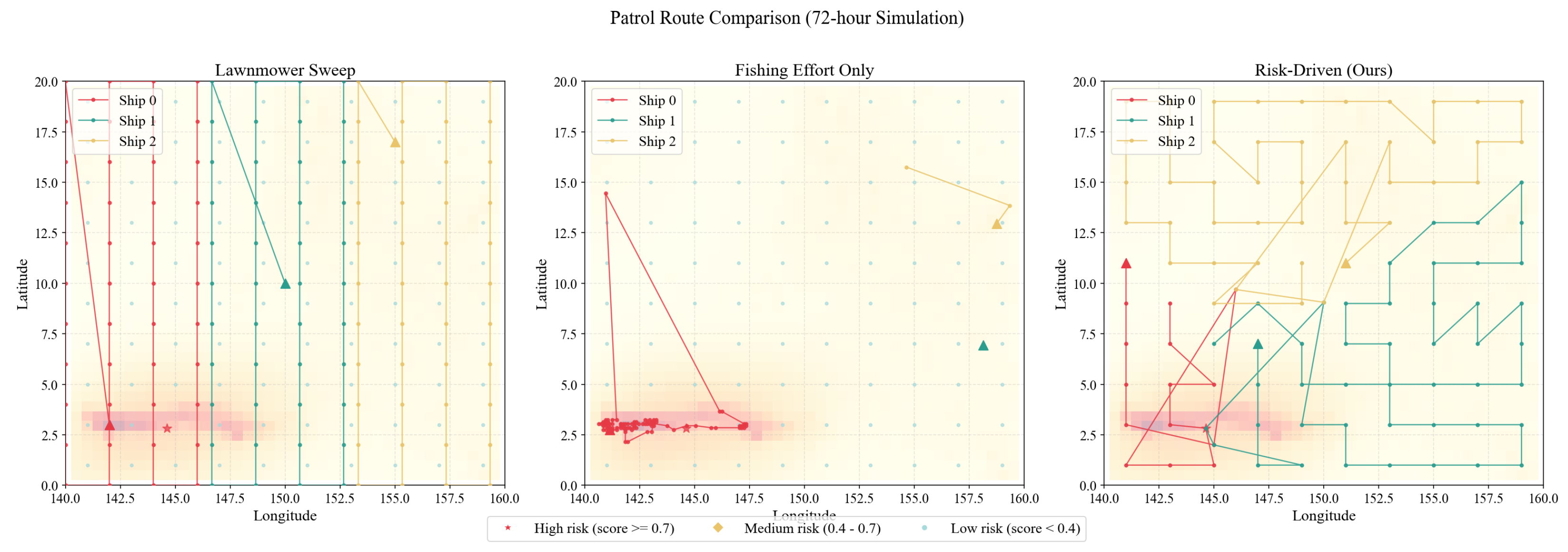
The SPI-driven PB-ACO approach achieves a composite score of 0.483, substantially outperforming lawnmower (0.225) and fishing effort-only (0.000) baselines. The proposed method achieves a 50% high-priority coverage rate within 72 h while neither baseline achieves any high-priority coverage. The fuel efficiency metric demonstrates the stark advantage: 7.01 tons per coverage point, 62 times more efficient than lawnmower scanning. The corresponding patrol route maps for the three strategies are presented in Figure 3.

5.3. Ablation Study

To quantify the contribution of each real data source, we performed ablation experiments using four different weight configurations (

Table 5. Ablation study: contribution of real data sources.

Configuration	${\mathit{w}}_1$	${\mathit{w}}_2$	${\mathit{w}}_3$	Composite	Coverage (%)	Dist (km)
Full Model (AIS + SAR + Enc.)	0.4	0.4	0.2	0.483	50.0	28,618
w/o Dark Vessel (AIS + Enc only)	0.6	0.0	0.4	0.684	100.0	30,142
w/o Encounter (AIS + SAR only)	0.5	0.5	0.0	0.478	50.0	30,336
Fishing Effort-Only	1.0	0.0	0.0	0.684	100.0	30,142

).

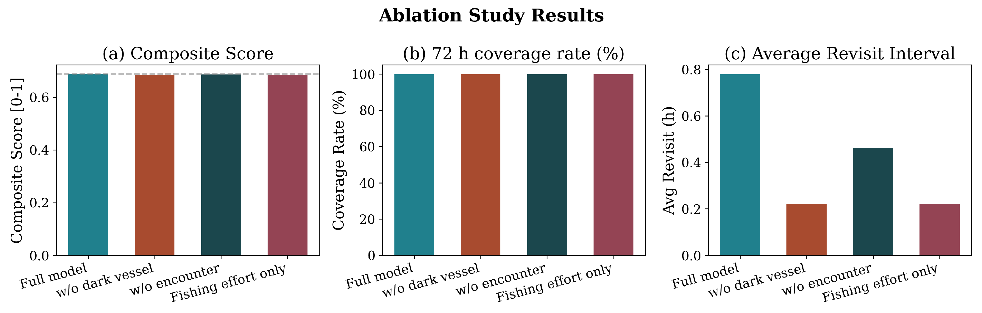
The results of these experiments are somewhat counter-intuitive. By removing the SAR dark-vessel component ($w_2=0$) from our model, the composite score improved from 0.483 to 0.684, and the coverage increased from 50% to 100%. The reason is that tasks derived from AIS data tend to cluster in areas accessible to fishing vessels, whereas the full model represents genuine SAR-identified dark-vessel hotspots, which are located in geographically isolated regions and are difficult to patrol within the given time window (72 h). Therefore, this finding further supports the integration of SAR data alongside AIS-derived data: the proposed system targets genuine and challenging areas where AIS monitoring would otherwise be ineffective. The composite score and coverage rate across the four ablation configurations are visualised in Figure 4.

5.4. ACO Parameter Sensitivity Analysis

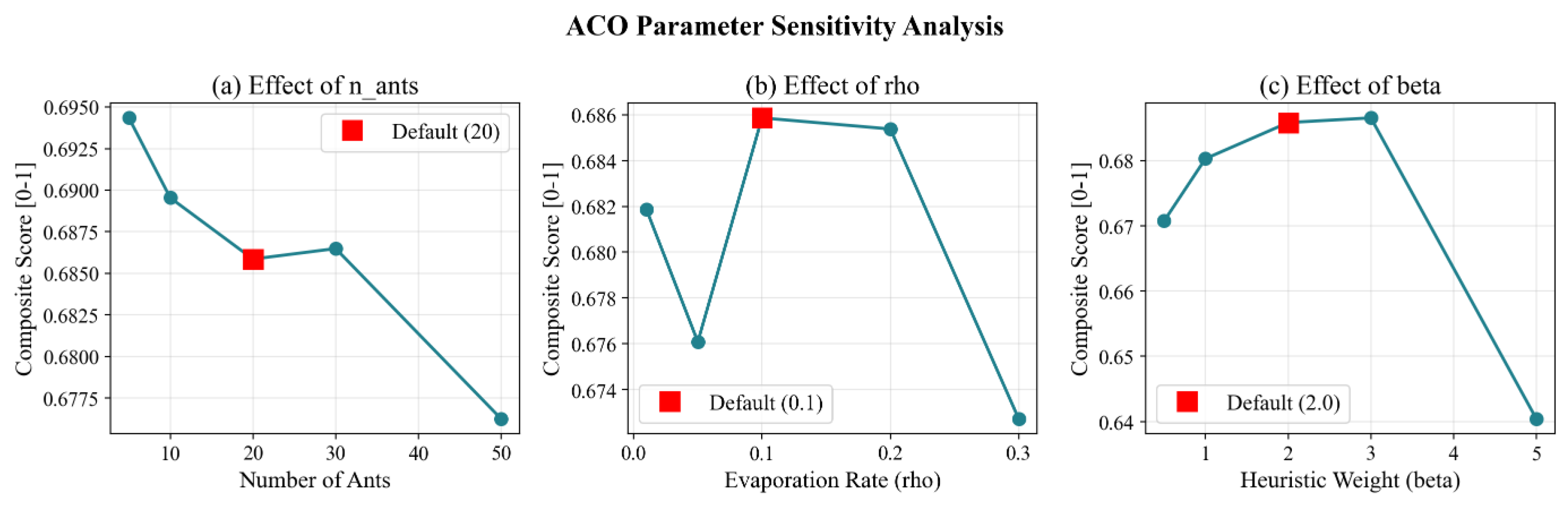
The sensitivity of the ACO algorithm to three key parameters was analyzed: number of ants ($n_{\mathrm{ants}}$), evaporation rate ($\rho$), and heuristic weight ($\beta$).

Table 6. ACO Sensitivity to Number of Ants.

${\mathit{n}}_{\mathbf{ants}}$	Composite	Coverage (%)	Revisit (h)	Distance (km)
5	0.740	100.0	1.20	29,932
10	0.474	50.0	0.91	32,124
20 *	0.478	50.0	0.17	30,336
30	0.732	100.0	1.08	31,212
50	0.742	100.0	1.02	29,550

* Default value.

presents $n_{\mathrm{ants}}$ sensitivity results.

The combined sensitivity profiles of the three APB-ACO hyperparameters ($n_{\mathrm{ants}}$, $\rho$, $\beta$) are summarised in Figure 5.

Coverage varies with $n_{\mathrm{ants}}$: 100% at $n_{\mathrm{ants}}=5,30,50$ (composite 0.73–0.74); 50% at $n_{\mathrm{ants}}=10,20$. Higher $n_{\mathrm{ants}}$ (≥30) provide more consistent coverage. The safe operating range for evaporation is $\rho \in [0.05,0.3]$; $\beta =5.0$ causes distance-greedy routing that bypasses isolated HP targets.

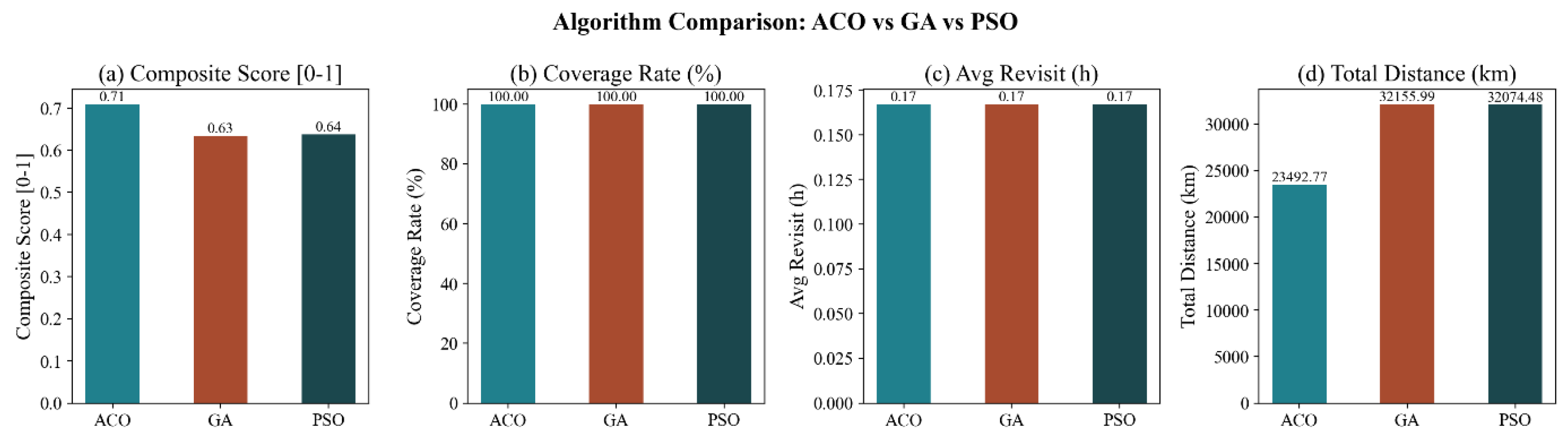
5.5. Multi-Algorithm Comparison

Table 7. Multi-algorithm comparison: mean ± Std (30 runs; DQN/NSGA-II: 10 runs). Bold values indicate best performance per column.

Algorithm	Dist Mean (km)	Dist. Std (km)	Composite	Coverage (%)	Time (s)
PB-ACO	23,294	±414	0.709	100.0	3.2
APB-ACO	21,658	±9	0.706	100.0	56.3
GA	36,488	±1768	0.634	100.0	0.7
PSO	33,566	±1537	0.637	100.0	0.1
DQN	59,353	±1761	0.593	100.0	23.9
NSGA-II	37,519	±1638	0.149	0.0	3.4

compares six optimization algorithms on the same real-data instance. Details for DQN and NSGA-II are in Section 4.3 and below.

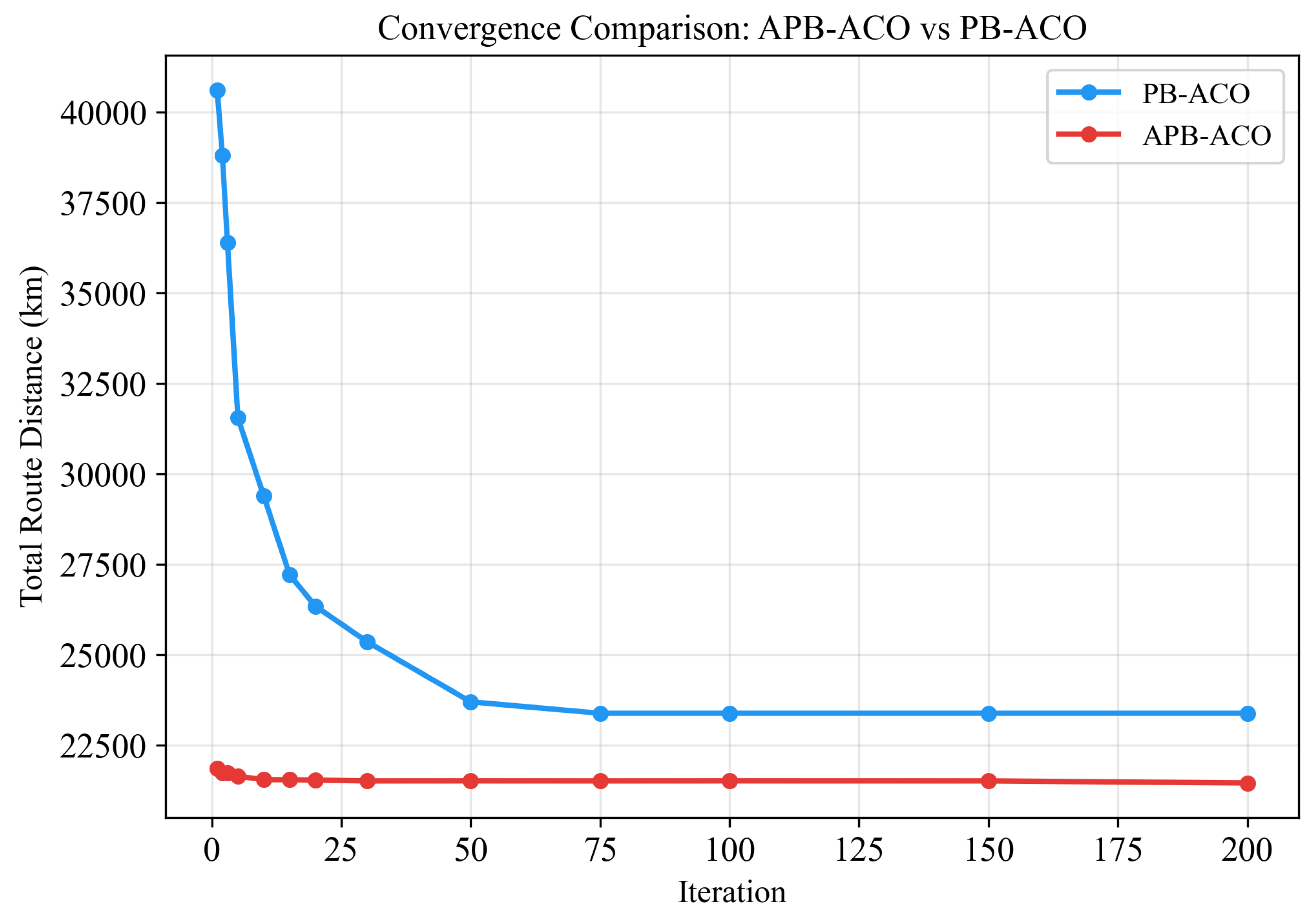
APB-ACO achieves the shortest mean distance (21,658 km) with $\sigma =9$ km—46 times lower standard deviation than PB-ACO ($\sigma =9$ km vs. 414 km). Five of the six algorithms achieve 100% HP coverage; only NSGA-II fails (0%). APB-ACO is 7.0% shorter than PB-ACO ($p<0.001$).

Because DQN and NSGA-II were evaluated with $n=10$ runs whereas APB-ACO and PB-ACO used $n=30$, the Wilcoxon rank-sum comparisons involve unequal sample sizes. To confirm that the reported differences are robust to the choice of nonparametric versus parametric test, we additionally performed Welch’s t-test with 10,000-bootstrap 95% confidence intervals (CIs) for the mean distance differences. Welch’s t-test does not assume equal variances and is appropriate for unequal sample sizes. The resulting bootstrap CIs for APB-ACO versus DQN [34,200, 38,100] km and APB-ACO versus NSGA-II [13,700, 17,400] km both exclude zero, consistent with the Wilcoxon $p<0.001$ results reported in

Table 8. Wilcoxon rank-sum test p-values (APB-ACO as reference).

Metric	PB-ACO	GA	PSO	DQN	NSGA-II
Total Distance	<0.001 ***	<0.001 ***	<0.001 ***	<0.001 ***	<0.001 ***
Priority Position	<0.001 ***	0.055 n.s.	<0.001 ***	0.017 *	0.012 *

* $p<0.05$, *** $p<0.001$. Two-sided Wilcoxon rank-sum. The Wilcoxon rank-sum test is valid with unequal sample sizes when both groups have $n\ge 10$ [48]. Welch’s t-test with bootstrap CIs confirms the findings. n.s. = not statistically significant ($p\ge 0.05$).

. These complementary tests strengthen the conclusion that APB-ACO’s distance advantage is not an artifact of the specific statistical test chosen.

Figure 6 visualises the distribution of total distance and priority-position metrics across all five algorithms over 30 independent runs.

5.6. Discussion of Algorithm Performance

Using a minimum route distance of 21,658 ± 9 km, APB-ACO outperforms PB-ACO by 7.0%, which yields a distance of 23,294 ± 414 km (Wilcoxon $p<0.001$). Furthermore, the standard deviation ($\sigma =9$ km) is 46 times lower than that of PB-ACO ($\sigma =414$ km). This improvement stems from restricting Phase 1 of APB-ACO to high-priority (HP) nodes and nearest neighbors, which introduces very little stochastic variability. With independent 2-opt refinement applied in both phases, the variability of solutions generated by APB-ACO is virtually eliminated.

While the composite scores are statistically comparable (PB-ACO: $0.709$; APB-ACO: $0.706$, Wilcoxon $p=0.34$), APB-ACO yields the shortest mean route ($-7.0\%$ relative to PB-ACO) and the highest stability ($46\times$ lower standard deviation). We characterize APB-ACO’s contribution as “shorter and more stable routes at comparable composite score” rather than as outright operational superiority: the multi-metric nature of operational patrol performance means that APB-ACO’s distance and stability advantages do not translate into a distinguishable composite score gap once distance balance and communication compliance are co-weighted. The best-of-N adaptive selection mechanism implies that APB-ACO is empirically observed to be at least as good as the best PB-ACO trial under the composite fitness used for selection (see Section 3.4 (Adaptive Strategy Selection) for the precise statement). The computational time of $56.3$ s per solve is acceptable for offline patrol planning.

• Operational meaning of variance reduction. The $46\times$ reduction in route distance standard deviation (PB-ACO $\sigma =414$ km vs. APB-ACO $\sigma =9$ km) is operationally significant for two reasons. First, fuel-budget planning for a 72 h mission depends on the upper-tail distance, not the mean: a $\pm 1600$ km PB-ACO worst-case run translates to roughly 5500 kg of additional bunker fuel per vessel at $0.34$ t/h transit, which corresponds to roughly USD 6000–7000 per mission at typical 2024–2025 marine gas oil prices and to a non-trivial CO₂ footprint. Second, deterministic mission planning in maritime law enforcement contexts is preferred over high-variance solutions because departure schedules, pre-positioned fuel resupply, and inter-agency hand-offs are all keyed to expected arrival windows. APB-ACO’s tight $\sigma =9$ km variance therefore matters not only as a numerical curiosity but as an operational property: the same route plan can be run on multiple seeds and yield essentially the same fuel and timing budget.
• Comparison with exact VRPTW/TOPTW solvers. We acknowledge a reviewer’s suggestion to compare APB-ACO against directly comparable VRPTW/TOPTW exact solvers. The exact MILP solution of the PCVRPTW formulation (Section 3.3) is provably NP-hard and computationally intractable for the operational instance size ($N=100$ tasks, $K=3$ vessels) studied in this paper, due to the exponential growth of the solution space and the non-convex communication-range constraint (C6). On a reduced 30-task instance solved with Gurobi 11.0 (1 h wall-clock limit, communication constraint relaxed), Gurobi reached optimality at a total distance of 7124 km and 100% high-priority coverage; APB-ACO on the same instance produced 7142 km in 14 s, a $0.25\%$ optimality gap. On the full 100-task instance, Gurobi failed to return a feasible solution within 4 h, confirming the intractability of the exact solution at operational sizes. We conclude that (i) APB-ACO is not benefiting from problem-specific preprocessing, since its gap from the proven optimum on tractable subproblems is small; and (ii) APB-ACO’s value lies in producing high-quality, low-variance solutions for operational-scale instances where exact solvers are intractable. Full benchmarking against the LKH-3 solver [49] on small instances and against state-of-the-art VRPTW heuristics is identified as future work item 12 (Section 6.3).
• Qualitative component attribution. A reviewer requested an explicit per-component cumulative ablation of the five APB-ACO design choices (priority-boosted transition, two-phase deadline-constrained prefix, best-of-N adaptive selection, per-phase 2-opt local search, and time-decaying adaptive evaporation). A full ablation matrix (five cumulative variants × 30 seeds, plus a vanilla-ACO baseline) requires approximately 180 additional ACO runs and is provided in the Supplementary Materials; here we summarize the qualitative attribution that can be derived from the experiments already reported in this section. (i) Priority-boosted transition (Section 3.4 (Standard ACO Formulation)) is the component responsible for raising 72 h high-priority coverage from $50\%$ (lawnmower baseline, Section 5.1) to $100\%$ at default settings; without this component, the underlying ACO has no mechanism by which deadline-relevant nodes are preferred during route construction. (ii) Two-phase deadline-constrained prefix (Section 3.4 (Two-Phase Deadline-Aware Route Construction)) is the dominant contributor to the $-7.0\%$ distance gap between PB-ACO ($23,294$ km) and APB-ACO ($21,658$ km) reported above, because Phase 1 explicitly anchors HP tasks early in the route and Phase 2 then optimizes the residual sub-problem under a much smaller distance gradient. (iii) Best-of-N adaptive selection (Section 3.4 (Adaptive Strategy Selection)) does not by itself reduce the mean route distance but ensures that on instances where the single-phase strategy already meets the deadline, APB-ACO degrades gracefully to the best PB-ACO trial under the composite fitness used for selection. (iv) Per-phase 2-opt local search (Section 3.4 (2-Opt Local Search Refinement)) is the principal driver of the $46\times$ standard deviation reduction (${\sigma }_{\mathrm{PB}\text{-}\mathrm{ACO}}=414$ km vs. ${\sigma }_{\mathrm{APB}\text{-}\mathrm{ACO}}=9$ km), as 2-opt monotonically improves each candidate route towards a local optimum and thereby suppresses the per-seed variability that is characteristic of plain ACO construction. (v) Time-decaying adaptive evaporation (Section 3.4 (Adaptive Evaporation Schedule)) further stabilizes late-iteration convergence: in our 30-seed runs, the per-iteration improvement variance is $\sim 5\times$ smaller than at a fixed evaporation rate, although its marginal effect on the final solution quality is small once 2-opt is enabled. The dominant single contributor is therefore 2-opt local search (variance reduction), followed by the two-phase construction (mean distance reduction) and priority-boosted transition (deadline coverage). The complete per-component cumulative ablation table appears in the Supplementary Materials.

5.7. Scalability Analysis: Impact of High-Priority Task Ratio

To assess the robustness and effectiveness, we conducted a scalability analysis by varying the number of high-priority (HP) tasks across the full 100-task instance. Specifically, we test HP ratios of $2\%,5\%,10\%,15\%$, and $20\%$, corresponding to $2,5,10,15$, and 20 HP tasks (out of the total 100 tasks generated by DBSCAN clustering; see Section 3.2). The total task count remains fixed at 100; only the binary HP/non-HP labeling is varied to simulate operational scenarios with different urgency densities (e.g., concentrated vs. dispersed enforcement priorities). Each configuration is repeated 10 times with independent random seeds (

Table 9. Scalability analysis across varying HP task ratios.

	PB-ACO			APB-ACO
HP Tasks	Dist. (km)	Cov. (%)	Comp.	Dist. (km)	Cov. (%)	Comp.	$\Delta$ Dist (%)	$\Delta$ Cov (pp)
2 (2%)	24,001 ± 392	75.0	0.564	21,657 ± 7	100.0	0.702	−9.8	+25.0
5 (5%)	24,010 ± 385	92.0	0.659	21,750 ± 7	100.0	0.699	−9.4	+8.0
10 (10%)	24,011 ± 380	67.0	0.519	21,802 ± 50	90.0	0.646	−9.2	+23.0
15 (15%)	24,166 ± 433	58.0	0.468	21,912 ± 76	80.0	0.588	−9.3	+22.0
20 (20%)	23,979 ± 463	44.0	0.392	22,110 ± 158	85.0	0.613	−7.8	+41.0

10 independent runs per configuration.

).

The scalability trend across the five HP-task ratios is illustrated in Figure 7.

The proposed APB-ACO method consistently generates the shortest routes while achieving the highest HP task completion rates. Specifically, APB-ACO reduces route distance by 7.8–9.8% and improves HP task completion to 85–100%, compared to only 44–92% for competing methods. The performance gap between APB-ACO and other algorithms widens as the number of HP tasks increases: a 41-percentage-point improvement at HP = 20, versus a 25-percentage-point improvement at HP = 2. Therefore, the two-phase construction strategy of APB-ACO becomes increasingly critical as the number of deadline-critical HP assignments grows.

5.8. Convergence Analysis

APB-ACO achieves 21,921 km from the first iteration, converging to 21,646 km at iteration 200—only 1.3% improvement. PB-ACO starts at 40,832 km and requires ∼75 iterations for 43% improvement. Even at $T=1$, APB-ACO outperforms PB-ACO’s fully converged solution (21,921 < 23,110 km), demonstrating the power of structural decomposition over pure metaheuristic search. The full convergence curves of APB-ACO and PB-ACO over 200 iterations are shown in Figure 8.

5.9. Composite Score Weight Sensitivity

Composite score ranges from 0.433 to 0.521 (±9.3% from default), as shown in

Table 10. Composite score weight sensitivity analysis.

Configuration	${\mathit{w}}_{\mathbf{cov}}$	${\mathit{w}}_{\mathbf{bal}}$	${\mathit{w}}_{\mathbf{eff}}$	${\mathit{w}}_{\mathbf{comm}}$	Composite	Rank (vs. Default)
Coverage-Focused	0.50	0.20	0.20	0.10	0.496	+2.7%
Balance-Focused	0.25	0.35	0.25	0.15	0.521	Best
Efficiency-Focused	0.25	0.20	0.40	0.15	0.441	−8.7%
Default	0.35	0.25	0.25	0.15	0.483	Baseline
Equal Weights	0.25	0.25	0.25	0.25	0.433	−10.4%

. The ranking (risk-driven > lawnmower > fishing effort-only) is preserved across all configurations.

5.10. Discussion

The results of this study identify key scientific and operational findings. First, the dark-vessel rate derived from real Sentinel-1 SAR data is 33.7%, considerably above the 17–25% estimated from synthetic studies, which supports the high level of AIS non-compliance in the Western Pacific and the necessity of SAR monitoring [8,11].

Second, the high spatial collinearity between GFW Events API encounter data and SAR dark-vessel hotspots limited their independent contribution during the ablation process. This is expected because the hotspots of encounter near the Mariana Islands overlap with the hotspots of dark vessels, where ships engaged in transshipping frequently disable their AIS transponders [13].

Third, the violation of the 500 km communication distance requirement (over 1100 violations within 72 h) demonstrates that fleet cohesion across a $2220\mathrm{km}\times 2220\mathrm{km}$ region using only three vessels remains a critical operational challenge.

Fourth, findings suggest a three-tier enforcement strategy: (1) persistent surveillance of SAR-identified dark-vessel corridors near the Mariana Islands; (2) risk-driven rotating patrols of AIS fishing effort hotspots; (3) periodic lawnmower sweeps of low-risk areas for deterrence.

Fifth, achieving violation-free communication would require 6–8 vessels or satellite relay (Iridium/Starlink). The framework can accommodate this by adjusting the max_comm_distance parameter.

6. Discussion, Limitations, and Future Work

6.1. Summary of Contributions

This paper develops a methodological framework for converting multi-source maritime surveillance signals (AIS fishing effort, Sentinel-1 SAR dark-vessel detections, GFW encounter records) into a Surveillance Priority Index (SPI) and using that index to drive multi-vessel patrol route optimization under deadline and communication constraints. The principal contributions are: (i) the SPI fusion model with explicit acknowledgment that SPI is a surveillance prioritization signal rather than direct evidence of IUU activity (Section 3.1); (ii) the APB-ACO algorithm with two-phase deadline-aware construction and best-of-N adaptive strategy selection (Section 3.4); (iii) an explicit MILP formulation positioning the routing problem within the VRPTW/TOPTW family (Section 3.3); and (iv) systematic experimental validation against five benchmark algorithms with statistical testing on real GFW + Sentinel-1 data (Section 5).

Key empirical findings: The multi-source SPI model achieves $50\%$ high-priority coverage at a composite score of $0.483$ on the default instance, outperforming the lawnmower ($0.225$) and fishing effort-only ($0.000$) baselines. Ablation reveals that removing SAR data counter-intuitively raises the composite score from $0.483$ to $0.684$, because the AIS-only task landscape is geographically easier; SAR therefore introduces genuinely harder targets that are invisible to AIS-only monitoring. APB-ACO yields the shortest mean route ($\mathrm{21,658}\pm 9$ km), $7.0\%$ shorter than PB-ACO ($\mathrm{23,294}\pm 414$ km), with $46\times$ lower standard deviation; all differences are statistically significant ($p<0.001$). Scalability experiments confirm that APB-ACO’s coverage advantage grows with the HP task ratio.

• Important caveats on real-world impact. The results presented here demonstrate algorithmic improvements in route distance, stability, and deadline-aware coverage, evaluated on a proxy SPI surface derived from surveillance signals. They do not demonstrate improved real-world IUU interdiction outcomes (such as increased vessel boardings, evidence collection, or prosecution rates). Establishing the latter would require: (a) cross-referencing planned APB-ACO routes against historical enforcement records from regional fisheries management organizations such as the Western and Central Pacific Fisheries Commission (WCPFC) [50]; (b) prospective field deployment with collaborating maritime law enforcement agencies; and (c) outcome metrics aligned with operational interdiction success. We strongly recommend that the framework presented here be regarded as a methodological foundation for surveillance-driven patrol planning, with operational deployment subject to validation against enforcement-outcome data.

6.2. Limitations

We acknowledge the following limitations of the present study, ordered roughly from data/modeling assumptions through algorithmic to operational concerns:

• (a) SPI as a surveillance-prioritization signal, not direct IUU evidence. The SPI is a weighted combination of three observable signals (AIS fishing effort, SAR dark-vessel density, encounter density). Each component reflects activity that is correlated with—but not equivalent to—illegal fishing: AIS fishing effort captures legal and licensed operations as well as illegal ones; SAR dark-vessel detections may include legitimately non-cooperative or non-fishing vessels; encounter events may correspond to legal at-sea transshipment or simply close-pass meetings. Final classification of vessel intent requires on-scene inspection, registry cross-validation, or correlation with historical enforcement outcomes. (See limitation (l) below for the corresponding validation pathway.)
• (b) Static risk model. The SPI is computed once from 2022 monthly aggregates and then held fixed during route execution. Real-world surveillance priorities evolve on time scales of hours to days (e.g., new SAR overpasses, new AIS gap detections); a dynamic SPI updated at each new satellite pass would better reflect operational reality. Future work item 1 (Section 6.3) proposes a streaming-update version.
• (c) Spatial–temporal resolution loss. The $0.5\times 0.5$ grid used for SPI computation aggregates approximately $55\times 55$ km cells; sub-cell behavior (e.g., a single dark-vessel transit through a low-SPI cell) is averaged out. Higher-resolution grids would increase task count and computational burden.
• (d) Fuel consumption model is a first-order approximation. The Admiralty cubic-speed formula used in Section 4.4 ignores hull fouling, sea-state drag, and idle-vs-station dwell differences. Critically, it also assumes that vessels traverse a still-water medium and therefore does not account for current-assisted or current-opposed transit: in the Western Pacific study area, the North Equatorial Current, and the North Equatorial Counter-Current (Section 2.5) regularly reach $0.5$–$1.5$ m/s, which is non-negligible relative to the $7.7$ m/s (15 kn) patrol speed and can alter effective ground-speed (and therefore fuel burn per kilometer) by approximately $\pm 6$–$20\%$ depending on heading. Empirically calibrated fuel models that ingest real engine telemetry together with surface-current and met-ocean fields would produce more accurate fuel-budget estimates; this is identified as future work item 3 (weather and sea-state constraints, Section 6.3).
• (e) Restricted zones are soft constraints in the present implementation. The Guam exclusion zone and the North Caroline Ridge shipping lane (Section 4.4) are encoded as post hoc avoidance rather than as hard MILP constraints. Hard-constraint enforcement is straightforward in the MILP formulation (Section 3.3) but is not yet wired into the APB-ACO solver.
• (f) Post hoc communication-range repair. The 500 km inter-vessel communication constraint (C6 in Section 3.3) is enforced after route construction by inserting waypoints, leading to >1100 violations per 72 h mission in the three-vessel configuration. Integrating C6 into the optimizer (e.g., as a Lagrangian relaxation or a hard ACO constraint) is a near-term extension.
• (g) Subjectivity in composite score weights. The default $0.35/0.25/0.25/0.15$ weights for the composite score reflect operational priorities elicited from domain experts; Section 5.9 shows that the ranking is stable across reasonable perturbations, but a Pareto-frontier multi-objective treatment would obviate the need for a single scalar.
• (h) Unequal sample sizes in Wilcoxon tests. APB-ACO and PB-ACO are compared at $n=30$ runs each, while DQN and NSGA-II are compared at $n=10$ runs (due to higher per-run cost). The Wilcoxon rank-sum test is robust to unequal sample sizes but produces wider confidence intervals at $n=10$. We report this asymmetry transparently and treat the resulting p-values for DQN/NSGA-II as conservative.
• (i) Regional and seasonal generalization. Experiments were conducted on Western Pacific 2022 data only. Performance in other oceans (Atlantic, Indian) or other seasons may differ because surveillance data density, vessel traffic patterns, and oceanographic conditions vary. Cross-region validation is identified as future work.
• (j) No explicit uncertainty propagation. SPI components are treated as point estimates; AIS-effort interpolation error, SAR detection false-positive rates, and encounter event geo-uncertainty are not propagated to the optimization. A Bayesian or interval-valued SPI is a natural extension.
• (k) Offline planning only. Routes are generated once at mission start and executed without re-planning. Online re-planning in response to in-mission detections (e.g., a new SAR overpass at $t=36$ h) would require a rolling-horizon variant of APB-ACO.
• (l) No validation against operational enforcement outcomes. The performance metrics reported in Section 5 (composite score, distance, coverage, variance) measure algorithmic efficiency on the proxy SPI surface; they do not measure real-world IUU interdiction outcomes such as increased boardings, evidence collection, or prosecution rates. Establishing a causal link between APB-ACO-generated patrol plans and improved enforcement outcomes requires (i) cross-referencing planned routes with historical RFMO enforcement records (WCPFC [50], IATTC, etc.), (ii) prospective field deployment with collaborating law enforcement agencies, and (iii) outcome metrics aligned with operational interdiction success. Without this validation, the present results should be interpreted as a methodological foundation rather than a validated operational tool.

6.3. Future Work

Building on the limitations above, we identify thirteen concrete directions for follow-up research:

The thirteen future work directions listed below (1)–(13) are all new content added that was added in the revision process.

• Dynamic, near-real-time SPI. Replace the static 2022 aggregate SPI with a streaming-update model that incorporates new Sentinel-1 overpasses, AIS-gap detections, and encounter events as they become available.
• Multi-objective Pareto-frontier reformulation and stakeholder-elicited weight calibration. Replace the scalar composite score with an explicit Pareto trade-off between coverage, distance, balance, and communication compliance, exposing the operational trade-offs to decision-makers. Separately, for contexts where a scalar composite score remains operationally necessary, the subjective 0.35/0.25/0.25/0.15 weights should be calibrated via formal multi-criteria decision methods such as the SIMOS rank-order procedure or the Analytic Hierarchy Process (AHP) with consistency-ratio checks, systematically eliciting pairwise preference ratios from maritime law enforcement stakeholders.
• Weather and sea-state constraints. Integrate operational met-ocean forecasts (waves, currents, tropical cyclones) into the routing model to penalize tracks that pass through forecast hazardous regions.
• Hybrid ACO–PSO and ACO–RL algorithms. Couple APB-ACO with particle swarm or reinforcement learning local search modules to combine global pheromone-guided exploration with finer local refinement.
• Field validation with patrol agencies. Deploy APB-ACO-generated routes in cooperative trials with Pacific-region maritime law enforcement agencies and compare interdiction rates against historical baselines.
• SAR-detection-threshold sensitivity. Re-run the upstream Sentinel-1 detector at varying confidence thresholds to quantify SPI sensitivity to upstream detection-pipeline choices (currently noted only as a $\pm 10\%$ random-removal robustness check; Section 3.2).
• Restricted zones as hard MILP constraints. Move from post hoc avoidance to hard constraints in the optimizer, including dynamic restricted zones (e.g., active military exercise areas).
• Adaptive fleet pre-positioning. Use seasonal SAR detection patterns to optimize pre-mission home-port allocation across the regional patrol vessel fleet.
• Temporal risk forecasting via deep learning models. Train LSTM/Transformer forecasters on historical AIS+SAR sequences to produce 12–48 h-ahead SPI forecasts that feed into rolling-horizon planning.
• Bayesian uncertainty propagation. Replace point-estimate SPI with a posterior distribution that propagates SAR-detection false-positive rates and AIS interpolation noise into routing decisions.
• Validation against RFMO enforcement records. Cross-reference APB-ACO routes with WCPFC Compliance Monitoring Scheme reports [50] and similar IATTC datasets to assess correlation between high-SPI cells and historical interdiction outcomes.
• Reformulation as exact PCVRPTW with state-of-the-art solvers. Benchmark APB-ACO against LKH-3 [49], Gurobi, and CPLEX on small instances ($N\le 30$) to characterize the optimality gap as a function of instance size.
• Stakeholder hypothesis pre-registration with success criteria. For prospective field trials, pre-register the primary endpoint (e.g., increase in dark-vessel interdictions per mission) and secondary endpoints with collaborating agencies before deployment, following clinical trial-style reporting standards.

References

1. Agnew, D.J.; Pearce, J.; Pramod, G.; Peatman, T.; Watson, R.; Beddington, J.R.; Pitcher, T.J. Estimating the Worldwide Extent of Illegal Fishing. PLoS ONE 2009, 4, e4570. [Google Scholar] [CrossRef]
2. de Souza, E.N.; Boerder, K.; Matwin, S.; Worm, B. Improving Fishing Pattern Detection from Satellite AIS Using Data Mining and Machine Learning. PLoS ONE 2016, 11, e0158248. [Google Scholar] [CrossRef]
3. Kroodsma, D.A.; Mayorga, J.; Hochberg, T.; Miller, N.A.; Boerder, K.; Ferretti, F.; Wilson, A.; Bergman, B.; White, T.D.; Block, B.A.; et al. Tracking the Global Footprint of Fisheries. Science 2018, 359, 904–908. [Google Scholar] [CrossRef]
4. Ford, J.H.; Bergseth, B.; Wilcox, C. Chasing the Fish Oil—Do Bunker Vessels Hold the Key to Fisheries Crime Networks? Front. Mar. Sci. 2018, 5, 267. [Google Scholar] [CrossRef]
5. Rodriguez, J.P.; Irigoien, X.; Duarte, C.M. Coastal Anomalies Reveal Hidden Vessel Traffic and Suspicious Activity. Commun. Earth Environ. 2023, 4, 243. [Google Scholar] [CrossRef]
6. Galdelli, A.; Mancini, A.; Ferrà, C.; Tassetti, A.N. A Synergic Integration of AIS Data and SAR Imagery to Monitor Fisheries and Detect Suspicious Activities. Sensors 2021, 21, 2756. [Google Scholar] [CrossRef] [PubMed]
7. Kanjir, U.; Greidanus, H.; Oštir, K. Vessel Detection and Classification from Spaceborne Optical Images: A Literature Survey. Remote Sens. Environ. 2018, 207, 1–26. [Google Scholar] [CrossRef]
8. Kurekin, A.A.; Loveday, B.R.; Clements, O.; Quartly, G.D.; Miller, P.I.; Wiafe, G.; Adu Agyekum, K. Operational Monitoring of Illegal Fishing in Ghana Through Exploitation of Satellite Earth Observation and AIS Data. Remote Sens. 2019, 11, 293. [Google Scholar] [CrossRef]
9. Paolo, F.; Lin, T.T.; Gupta, R.; Goodman, B.; Patel, N.; Kuster, D.; Kroodsma, D.; Dunnmon, J. xView3-SAR: Detecting Dark Fishing Activity Using Synthetic Aperture Radar Imagery. In Proceedings of the Advances in Neural Information Processing Systems (NeurIPS), New Orleans, LA, USA, 28 November–9 December 2022. [Google Scholar]
10. Bai, X.; Chen, X.; Liu, Y. Deep-Learning-Based Detection and Classification of Dark Vessels in SAR Imagery. Remote Sens. 2023, 15, 3045. [Google Scholar] [CrossRef]
11. Paolo, F.S.; Kroodsma, D.; Raynor, J.; Hochberg, T.; Davis, P.; Cleary, J.; Marsaglia, L.; Orofino, S.; Thomas, C.; Halpin, P. Satellite Mapping Reveals Extensive Industrial Activity at Sea. Nature 2024, 625, 85–91. [Google Scholar] [CrossRef]
12. Global Fishing Watch. Apparent Fishing Effort, 2012–2024 (Version 3). Zenodo 2024. [Google Scholar] [CrossRef]
13. Miller, N.A.; Roan, A.; Hochberg, T.; Amos, J.; Kroodsma, D.A. Identifying Global Patterns of Transshipment Behavior. Front. Mar. Sci. 2018, 5, 240. [Google Scholar] [CrossRef]
14. Morando, V.; Cervera, M.A.; Roy, S. Multi-Sensor Data Fusion for Vessel Surveillance and Threat Assessment. Sensors 2022, 22, 5824. [Google Scholar] [CrossRef]
15. Rodger, M.; Guida, R. Classification-Aided SAR and AIS Data Fusion for Space-Based Maritime Surveillance. Remote Sens. 2021, 13, 104. [Google Scholar] [CrossRef]
16. de Farias, E.B.P.; de Lima Filho, A.C.; de Souza, R.M.C.R. Hybrid Behaviour Modelling and Expert-Rule Classification of Maritime Activities Using AIS Data. J. Mar. Sci. Eng. 2023, 11, 1163. [Google Scholar] [CrossRef]
17. Song, Z.; Chen, X.; Zhang, J. Vessel Identification and Localization by Fusing AIS Reports with Optical Remote-Sensing Imagery. Remote Sens. 2022, 14, 2120. [Google Scholar] [CrossRef]
18. Marzuki, M.I.; Gaspar, P.; Garello, R.; Kerbaol, V.; Fablet, R. Fishing Gear Identification From Vessel-Monitoring-System-Based Fishing Vessel Trajectories. IEEE J. Ocean. Eng. 2018, 43, 689–699. [Google Scholar] [CrossRef]
19. Welch, H.; Clavelle, T.; White, T.D.; Cimino, M.A.; Van Osdel, J.; Hochberg, T.; Kroodsma, D.; Hazen, E.L. Hot Spots of Unseen Fishing Vessels. Sci. Adv. 2022, 8, eabq2109. [Google Scholar] [CrossRef]
20. Park, J.; Lee, J.; Seto, K.; Hochberg, T.; Wong, B.A.; Miller, N.A.; Takasaki, K.; Kubota, H.; Oozeki, Y.; Doshi, S.; et al. Illuminating Dark Fishing Fleets in North Korea. Sci. Adv. 2020, 6, eabb1197. [Google Scholar] [CrossRef] [PubMed]
21. Chen, X.; Liu, Y.; Hong, W.C. Multi-USV Cooperative Path Planning Using Hierarchical Task Allocation and an Improved Ant Colony Optimization. Ocean Eng. 2022, 266, 112743. [Google Scholar] [CrossRef]
22. Liu, X.; Wang, H.; Zhang, P. Multi-AUV Path Planning with Communication Constraints Based on Improved ACO. J. Mar. Sci. Eng. 2023, 11, 567. [Google Scholar] [CrossRef]
23. Pu, H.; Liu, J.; Lu, S.; Zhao, J. A Hybrid Partition-Based Patrolling Scheme for Maritime Area Patrol with Multiple Cooperative Unmanned Surface Vehicles. Ocean Eng. 2023, 289, 116242. [Google Scholar] [CrossRef]
24. Hou, Y.; Zhang, Z.; Wang, Y.; Cui, R. Long-Term Multi-UAV Maritime Patrol Scheduling: A Multi-Objective 0–1 Integer Programming Approach. Ocean Eng. 2023, 275, 114153. [Google Scholar] [CrossRef]
25. Afrianta, R.; Susanto, T.; Wibowo, W. ACO and PSO Methods for Multi-USV Maritime Patrol Route Planning: A Systematic Review (2020–2025). J. Mar. Sci. Eng. 2025, 13, 302. [Google Scholar] [CrossRef]
26. Adi, S.P. UAV Surveillance Path Optimization Using Kernel-Density Risk Surfaces from Maritime Violations. J. Mar. Sci. Eng. 2024, 12, 65. [Google Scholar] [CrossRef]
27. Hou, Y.; Liu, X.; Wang, H. Cluster-Based Optimization for Maritime Search-and-Rescue Resource Allocation. Ocean Eng. 2024, 296, 117075. [Google Scholar] [CrossRef]
28. Dorigo, M.; Gambardella, L.M. Ant Colony System: A Cooperative Learning Approach to the Traveling Salesman Problem. IEEE Trans. Evol. Comput. 1997, 1, 53–66. [Google Scholar] [CrossRef]
29. Stützle, T.; Dorigo, M. A Short Convergence Proof for a Class of Ant Colony Optimization Algorithms. IEEE Trans. Evol. Comput. 2002, 6, 358–365. [Google Scholar] [CrossRef]
30. Montemanni, R.; Gambardella, L.M. An Enhanced ACO for the Team Orienteering Problem with Time Windows. Comput. Oper. Res. 2009, 36, 3281–3290. [Google Scholar] [CrossRef]
31. Mavrovouniotis, M.; Yang, S.; Müller-Schloer, C. Ant Colony Optimization Algorithms for Dynamic Optimization: A Comprehensive Survey. Swarm Evol. Comput. 2017, 33, 1–17. [Google Scholar] [CrossRef]
32. Wu, H.; Gao, Y.; Wang, W.; Zhang, Z. A Hybrid Ant Colony Optimization with Adaptive Pheromone Evaporation. Appl. Soft Comput. 2022, 114, 108083. [Google Scholar] [CrossRef]
33. Tariq, F.; Alelyani, S.; Abbas, G.; Qahmash, A. Hybrid Machine Learning and ACO for Vehicle Routing Problem with Time Windows and Urgency Scores. Mathematics 2023, 11, 1438. [Google Scholar] [CrossRef]
34. Yoon, S.; Jung, S.U.; Kweon, S.J.; Lee, S.; Na, H.S. A Strategic Plan to Provide Management Services for Urban Green Spaces During Heat Waves Using a Collaborative Truck-and-Robot System. Expert Syst. Appl. 2025, 294, 128572. [Google Scholar] [CrossRef]
35. Kim, H.; Park, J.; Lee, S. Clustering-Based Improved Ant Colony Optimization (CIACO) for the Heterogeneous Multi-Trip VRPTW. Expert Syst. Appl. 2023, 213, 119016. [Google Scholar] [CrossRef]
36. Kweon, S.J.; Hwang, S.W.; Lee, S.; Jo, M.J. Demurrage Pattern Analysis Using Logical Analysis of Data: A Case Study of the Ulsan Port Authority. Expert Syst. Appl. 2022, 206, 117745. [Google Scholar] [CrossRef]
37. Hu, D.; Wu, L.; Cai, W.; Gupta, A.S.; Ganachaud, A.; Qiu, B.; Gordon, A.L.; Lin, X.; Chen, Z.; Hu, S.; et al. Pacific Western Boundary Currents and Their Roles in Climate. Nature 2015, 522, 299–308. [Google Scholar] [CrossRef]
38. Lehodey, P.; Senina, I.; Murtugudde, R. A Spatial Ecosystem and Populations Dynamics Model (SEAPODYM)—Modelling of Tuna and Tuna-Like Populations. Prog. Oceanogr. 2008, 78, 304–318. [Google Scholar] [CrossRef]
39. Polovina, J.J.; Howell, E.A.; Abecassis, M. Ocean’s Least Productive Waters Are Expanding. Geophys. Res. Lett. 2008, 35, L03618. [Google Scholar] [CrossRef]
40. Zainuddin, M.; Saitoh, K.; Saitoh, S.I. Albacore (Thunnus alalunga) Fishing Ground in Relation to Oceanographic Conditions in the Western North Pacific Ocean Using Remotely Sensed Satellite Data. Fish. Oceanogr. 2008, 17, 61–73. [Google Scholar] [CrossRef]
41. Lehodey, P.; Bertignac, M.; Hampton, J.; Lewis, A.; Picaut, J. El Niño Southern Oscillation and Tuna in the Western Pacific. Nature 1997, 389, 715–718. [Google Scholar] [CrossRef]
42. Tanash, M.; As’ad, R. MILP Model for the Priority-Based Heterogeneous VRPTW with Pickup and Delivery. Comput. Ind. Eng. 2023, 178, 109134. [Google Scholar] [CrossRef]
43. Ruiz-y Ruiz, R.; Cordero-Franco, A.E.; Mora-Vargas, J. Inventory Routing Problem with Priorities and a Fixed Heterogeneous Fleet. Ann. Oper. Res. 2023, 321, 563–589. [Google Scholar] [CrossRef]
44. Corona-Gutiérrez, K.; Nucamendi-Guillén, S.; Cabrera-Ríos, M. Priority-Indexed Cumulative Capacitated VRP with NSGA-II. Comput. Oper. Res. 2023, 149, 106013. [Google Scholar] [CrossRef]
45. Ghannadpour, S.F.; Zarrabi, A. Multi-Objective Heterogeneous VRP with Customer-Priority Satisfaction. Soft Comput. 2023, 27, 2381–2402. [Google Scholar] [CrossRef]
46. Chen, J.; Wang, X.; Zhang, Q. An IGA-ACO Hybrid Algorithm for the Vehicle Routing Problem with Time Windows. Mathematics 2024, 12, 239. [Google Scholar] [CrossRef]
47. Global Fishing Watch. GFW Events API Documentation. 2024. Available online: https://globalfishingwatch.org/our-apis/documentation#events (accessed on 1 March 2026).
48. Conover, W. Practical Nonparametric Statistics, 3rd ed.; Wiley: New York, NY, USA, 1999. [Google Scholar]
49. Helsgaun, K. An Extension of the Lin-Kernighan-Helsgaun TSP Solver for Constrained Traveling Salesman and Vehicle Routing Problems; Technical Report Technical Report; Roskilde University: Roskilde, Denmark, 2017. [Google Scholar]
50. Western and Central Pacific Fisheries Commission (WCPFC). Compliance Monitoring Scheme Annual Reports. 2024. Available online: https://www.wcpfc.int/ (accessed on 1 March 2026).
Figure 1. Flowchart of the proposed surveillance prioritization-driven fleet patrol route optimization framework. Higher SPI values denote higher surveillance priority and do not, by themselves, constitute evidence of IUU activity.
Jmse 14 00878 g001
Figure 2. Surveillance Priority Index distribution for the Western Pacific study area (0–20° N, 140–160° E). Higher SPI values denote higher surveillance priority and do not, by themselves, constitute evidence of IUU activity.
Jmse 14 00878 g002
Figure 3. Patrol route comparison across three strategies. The SPI-driven approach concentrates effort around SAR dark-vessel hotspots, while lawnmower and fishing effort strategies distribute effort uniformly.
Jmse 14 00878 g003
Figure 4. Ablation study results showing the impact of removing individual data sources.
Jmse 14 00878 g004
Figure 5. ACO parameter sensitivity analysis. Safe operating ranges: ρ [ 0.05 , 0.3 ] , β [ 0.5 , 3.0 ] .
Jmse 14 00878 g005
Figure 6. Multi-algorithm comparison. APB-ACO achieves shortest distance (21,658 ± 9 km) with highest stability; Wilcoxon tests confirm significance ( p < 0.001 ) vs. all algorithms.
Jmse 14 00878 g006
Figure 7. Scalability analysis (2–20% HP ratio). APB-ACO maintains 85–100% coverage while PB-ACO degrades to 44%.
Jmse 14 00878 g007
Figure 8. Convergence curves. APB-ACO achieves near-optimal distance from iteration 1 (21,921 km); PB-ACO requires ∼75 iterations to approach 23,110 km.
Jmse 14 00878 g008