Abstract
Effective fishery management in coastal waters requires accurate assessments of species–environment relationships, particularly in data-rich but zero-inflated contexts (i.e., datasets with an excess of zero catches). Here, we used fishery-independent trawl survey data collected from 2018 to 2019 in the offshore waters of southern Zhejiang Province of China to investigate the spatio-temporal distribution of Setipinna taty (scaly hairfin anchovy) and its environmental determinants. Given the high frequency of zero catches, we fitted both zero-inflated Poisson (ZIP) and zero-inflated negative binomial (ZINB) models and selected the best-performing approach using the Akaike information criterion (AIC). Cross-validation indicated that the ZINB model (RMSE: 199.1, R2; 0.25) outperformed ZIP model (RMSE: 239.4, R2; 0.23). Temperature, depth, and salinity were key predictors of S. taty abundance, which generally occurred at depths of 20–40 m and salinities of 26–34 psu. We then applied the optimal ZINB model to predict S. taty distributions in spring, summer, and autumn of 2020. The predictions indicated a summer peak in abundance and a nearshore-to-offshore decreasing gradient, and were broadly consistent with the spatial distribution trends observed in the 2020 survey data. The highest predicted densities were located in nearshore areas off Wenzhou and Taizhou, west of 122° E. By clarifying the key environmental factors shaping S. taty distribution and applying zero-inflated count models to account for an excess of zero catches, which occur more frequently than expected under standard negative binomial models, this study provides an improved basis for effective conservation and sustainable utilization of S. taty resources in the southern offshore waters of Zhejiang; nevertheless, predictive performance could be further improved by incorporating additional environmental and biotic covariates together with extended spatio-temporal data.
1. Introduction
Over the past few decades, fishing pressure and associated anthropogenic disturbances, including coastal development and engineering activities, pollution inputs, and trawling-related habitat disturbance, have significantly altered marine ecosystems in China’s coastal waters [1,2]. Continued exploitation of large, high-trophic-level species has been accompanied by increasing catches of smaller, lower-trophic-level pelagic fish, a pattern often described as “fishing down the food web” [3]. This shift can profoundly affect population dynamics, trophic interactions, and overall ecosystem resilience. In recent years, small pelagic fish have increasingly dominated commercial catches [2], underscoring the urgent need to investigate their population dynamics, ecological roles, and implications for resource management.
Due to the influence of human activities, traditional fishery resources have been highly exploited and utilized, and species such as Setipinna taty have gradually emerged as the primary targets in these marine areas [4]. Setipinna taty, also known as the scaly hairfin anchovy, is a warm-water pelagic species of the family Engraulidae and is widely distributed along China’s coastline, including the Bohai Sea, Yellow Sea, East China Sea, and South China Sea [5,6,7]. In recent years, it has become one of the main contributors to fishery production in the East China Sea and the Yellow Sea [4]. Han et al. [5] proved that S. taty in the Bohai Sea was at an overfished level (of stock biomass) in 2019. However, due to the lack of data, the stock assessment of S. taty in different sea areas is still under study. Jin et al. [8] reported that the population structure of S. taty has tended towards younger cohorts of smaller fish. It usually grows up to 15 cm in length and is a pelagic spawner. Its spawning period is from February to April in the Yellow Sea and from May to June in the northern part of the East China Sea [9]. Occupying an intermediate trophic level, S. taty plays a vital ecological role in transferring energy and nutrients from planktonic prey (e.g., copepods, amphipods, shrimp larvae) to higher-trophic-level predators [5,10,11]. Consequently, fluctuations in S. taty populations can trigger trophic cascades that not only influence predator abundance but also disrupt broader marine ecosystem function and resilience.
The southern offshore waters of Zhejiang in the East China Sea lie in a warm-temperate marine zone, where the high-salinity Taiwan Warm Current converges with lower-salinity currents, creating a nutrient-rich environment that provides favorable conditions for the growth and reproduction of many fishery species [12,13]. Historically, these favorable conditions have supported high biodiversity and robust fisheries, positioning this region as an important fishery resource base. Temperature and salinity are widely recognized as key drivers of physiological processes in aquatic organisms. Changes in these variables can alter fish metabolic rates, growth, and behavior, and consequently influence habitat use and distribution patterns. Water depth is also an important determinant of habitat selection and may affect fish distribution indirectly by modifying associated environmental conditions, such as temperature and dissolved oxygen [14]. However, due to the pressure of fishing and habitat degradation, commercially important species have shown substantial declines in both abundance and body size [13]. Under these altered conditions, understanding the population dynamics and ecological functions of critical species like S. taty has become increasingly urgent for sustainable resource management and conservation.
Despite its ecological importance, quantitative assessments of S. taty populations are complicated by substantial zero-inflation in fishery-independent survey data, which are obtained from standardized scientific surveys conducted independently of commercial fishing, meaning that the number of zero observations is much higher than would be expected under standard count distributions. This pattern arises from the species’ schooling behavior, patchy distributions, seasonal migrations, and gear selectivity [15,16]. Standard Poisson and negative binomial regression models (used as the count component of ZIP/ZINB) assume that zeros are generated by the same process as positive counts and therefore often fail to accommodate an excess of zeros in the data. Consequently, these models can lead to biased parameter estimates and suboptimal predictions [17]. To address this challenge, zero inflated models, such as Zero-Inflated Poisson (ZIP) and Zero-Inflated Negative Binomial (ZINB), have been widely recommended for better handling overdispersed and zero-heavy data [18]. Here, zero inflation refers to a situation in which zero counts occur more frequently than would be expected under a standard Poisson regression model given the same mean structure. Unlike standard Poisson regression, which assumes all zeros and positive counts arise from a single Poisson process, the ZIP model introduces an additional zero-generating process to account for structural zeros, while modeling the remaining counts with a Poisson regression component [19]. ZIP model typically assumes that the occurrence frequency of an event follows a Poisson distribution, taking the frequency of occurrence at that time as the response variable and fitting a generalized linear Poisson regression model to explore the influence of explanatory variables on the event [19]. For discrete count data taking non-negative integer values, a ZINB model may be considered when the data exhibit both zero inflation and overdispersion, with variance exceeding the mean [18]. ZIP is suitable for zero-inflated count data when the variance is approximately equal to the mean, whereas the ZINB model accommodates zero inflation while allowing overdispersion through a negative binomial count component. Therefore, ZINB is often more appropriate for fishery survey count data that are both zero-inflated and overdispersed [20]. Cross-validation is commonly used to assess model stability, with predictive performance evaluated using metrics such as Root Mean Square Error (RMSE) and Coefficient of Determination (R2) [21]. Although extensively applied in disciplines such as epidemiology and finance [22,23], these methods remain relatively underutilized in marine ecological research in China. Internationally, zero-inflated models have proven effective in modeling rare or highly migratory species and evaluating bycatch risk [24,25]. Nonetheless, correct implementation requires carefully distinguishing structural absences from observation-induced zeros, as well as rigorous interpretation of model parameters [15,17].
In this study, we employ zero-inflated modeling approaches to investigate the abundance patterns and environmental drivers of S. taty in the coastal waters off southern Zhejiang. Using fishery-independent trawl survey data collected during 2018–2019, our specific objectives are to: (1) compare the performance of ZIP and ZINB models in predicting S. taty abundance, and use the best-fitting model to forecast spatiotemporal distributions in 2020; and (2) identify the key environmental determinants shaping the distribution of this ecologically pivotal forage fish. By integrating fishery-independent surveys with advanced statistical modeling and ecological theory, we aim to provide novel insights into the population dynamics and ecological role of S. taty under complex oceanographic conditions, ultimately informing sustainable resource management and ecosystem conservation.
2. Materials and Methods
2.1. Data Source
The research area is located in the central–southern part of the East China Sea and include the important Wenzhou–Taizhou fishing ground. This area belongs to the warm-temperate marine zone and is influenced year-round by both the low-salinity Zhejiang Coastal Current and the high-temperature, high-salinity Taiwan Warm Current [26]. The area is characterized by abundant nutrients and prey availability, and pronounced seasonal variations affect the spatial distribution patterns of fish species [27].
Fishery resource and environmental data were collected during a comprehensive fishery-independent trawl survey in four seasons (spring, summer, autumn, and winter) between 2018 and 2019 in the southern offshore waters of Zhejiang, China (Figure 1). To minimize ambiguity caused by regional differences in seasonal transitions, seasons in this study were defined based on the timing of the four annual survey cruises, specifically spring (May), summer (August), autumn (November), and winter (February). Sampling stations were fixed, and at each station, bottom trawling was conducted at speeds of 2–4 kn. The trawl mouth measured 40 m in width and 7.5 m in height. All specimens were identified to species level, and the catch for each species was recorded.
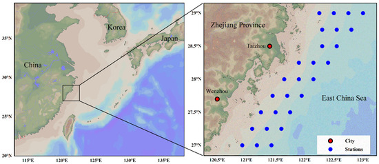
Figure 1.
Survey stations of fishery resources in the south offshore of Zhejiang, China.
The abundance of S. taty was standardized to individuals per square kilometer (ind·km−2) by account of a trawling duration of 1 h and an average speed of 3 knots. Standardized values were converted to non-negative integers using the ceiling function prior to ZIP/ZINB modeling. These procedures followed the Specifications for Oceanographic Survey (GB/T 12763) [28] and the Specification for Marine Monitoring (GB 17378) [29]. Environmental factors, including depth (Dep, m), temperature (Tem, °C), and salinity (Sal, psu), were measured using a WTW MultiLine Multi 3630 (Weilheim, Germany). The dataset used in this study included the standardized abundance index (AI) of S. taty, season, longitude (Lon, °E), latitude (Lat, °N), depth, temperature, and salinity. Across the four seasonal surveys conducted in 2018–2019, temperature ranged from 10.4–33.6 °C (mean: 21.3 °C), salinity ranged from 25.6–34.3 psu (mean: 31.7 psu), and sampling depth ranged from 17.6–71.1 m (mean: 48.8 m). In addition, variables such as chlorophyll a, turbidity, current velocity, and tidal direction may also be important for S. taty distribution; however, these variables were not included in the present study because they were not measured in our survey program and were therefore unavailable.
2.2. Data Characteristics
The dataset included many zero observations (i.e., stations with no recorded S. taty). In fishery-independent trawl surveys, such zeros may reflect true absence at a given station and time, but they can also occur when fish are present yet not captured because of patchy distributions, schooling behavior, and imperfect catchability (including gear selectivity). In our dataset, 61 of 216 samples were zeros (28.24%). To assess whether zeros were more frequent than expected under standard count models, we fitted baseline Poisson and negative binomial (NB) regressions using the same predictors as the subsequent zero-inflated models. For each observation, we used the fitted mean from the baseline model to compute the probability of observing a zero, and averaged these probabilities across all observations to obtain the expected zero proportion. The expected zero proportions were 0.26% (Poisson) and 24.24% (NB), both lower than the observed value, indicating excess zeros. Overdispersion was evaluated using the Poisson dispersion ratio (Pearson χ2/df), calculated as the sum of squared Pearson residuals divided by the residual degrees of freedom; the resulting value (293) indicated substantial overdispersion. Accordingly, we retained the zero observations and analyzed the data using zero-inflated count models (ZIP and ZINB).
2.3. Model Construction
2.3.1. Variable Screening
Fishery resource and environmental data from 2018–2019 were analyzed. Before fitting the models, the Variance Inflation Factor (VIF) was used to conduct multicollinearity tests on six environmental factors [30]. Variable with a VIF value greater than 5 were excluded from subsequent analyses [31]. In this study, longitude and latitude exceeded this threshold and were therefore removed; detailed VIF values are provided in Section 3.3.1 and Table 1. Different combinations of the remaining variables were then evaluated in the modeling process.

Table 1.
Multicollinearity test for predictive variables.
2.3.2. Model Selection
To handle the zero inflation often observed in count data, ZINB and ZIP models were considered. We first compared ZIP and ZINB using repeated five-fold cross-validation [21]. In each repetition, the dataset was randomly partitioned into five folds; models were trained on four folds (80%) and evaluated on the remaining fold (20%). This five-fold procedure was repeated 1000 times with different random partitions to obtain stable estimates of predictive performance. Model performance was summarized using RMSE and R2 calculated on the held-out folds. The model with consistently lower RMSE and higher R2 across repetitions was selected as the final modeling framework. For each test set, we quantified prediction accuracy using the root mean square error (RMSE): , where yi is the observed abundance and is the predicted abundance for observation i in the test set, and n is the number of test observations. Lower RMSE indicates better predictive accuracy.
We also assessed agreement between observed and predicted values by fitting a simple linear regression on the test set: , and reporting the slope a, intercept b, and coefficient of determination R2. Values of a close to 1 and b close to 0 indicate close agreement, and higher R2 indicates improved explanatory power.
After selecting the final model based on cross-validation, we evaluated all possible combinations of candidate environmental predictors and selected the optimal predictors using the Akaike Information Criterion (AIC) [32,33], defined as where L is the maximized likelihood and m is the number of estimated parameters. AIC balances goodness of fit (log-likelihood) against model complexity (parameter penalty); therefore, smaller AIC values indicate a better trade-off and reduce the risk of overfitting when comparing models fitted to the same dataset.
Zero-inflated models split the count process into two parts: a binomial process that models whether a zero or non-zero count occurs, and a conventional count process (Poisson or negative binomial) that models the positive counts [19]. Let yi denote the observed abundance (count) of S. taty at station i. The general form of a zero-inflated model can be written as:
where is the zero-inflation parameter indicating the probability of an “extra” zero and represents the probability mass function of the count distribution.
In this study, we considered both a zero-inflated Poisson model (ZIP) and a zero-inflated negative binomial model (ZINB). For ZIP, the count component follows a Poisson distribution with mean μi. For ZINB, the count component follows a negative binomial distribution with mean μi and dispersion parameter α. The model links were specified as:
where γ and β are regression coefficient vectors for the zero-inflation and count components, respectively, and xi and zi are covariable vectors, in our analysis, the same set of predictors was used for both components.
Candidate predictors included longitude (Lon; degrees), latitude (Lat; degrees), temperature (Tem; °C), salinity (Sal; psu), and depth (Dep; m). The model syntax for including all explanatory variables is:
Models were fitted by maximum likelihood using the zeroinfl () function in R (package pscl), with dist = “poisson” for ZIP and dist = “negbin” for ZINB. We evaluated all possible subsets of the candidate predictors and selected the final model as the combination that minimized the Akaike Information Criterion (AIC).
2.4. Spatio-Temporal Prediction of S. taty Distribution
To generate spatially continuous abundance maps for visualization, we performed kriging interpolation of station-based S. taty abundance values in spring, summer, and autumn 2020 using ArcGIS 10.3 at a spatial resolution of 0.05°. The resulting season-specific interpolated abundance surfaces were used to characterize seasonal variation in spatial distribution. Because no survey was conducted in winter 2020 due to the COVID-19 pandemic, neither environmental interpolation nor abundance prediction was carried out for that season. For clarity, the overall workflow of data processing, model fitting, validation, and prediction is summarized in the flowchart shown in Figure 2.
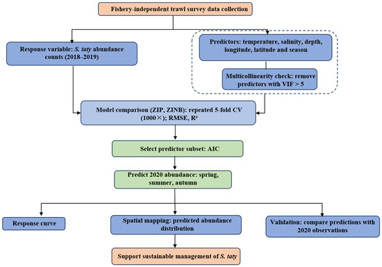
Figure 2.
Schematic overview of the data processing, modeling, validation, and prediction procedures. The dashed box indicates the predictor screening process.
Model fitting and prediction were performed in R 3.5.3 [21]. The zeroinfl () function from pscl R package (version 1.5.9) is used to fit the ZIP and ZINB models [34]. To facilitate direct comparison, the observed distributions of S. taty abundance from 2018–2019 were also visualized in ArcGIS and compared with the predicted patterns. All the figures were drawn, respectively, using R, ArcGIS and ocean data view.
3. Results
3.1. Seasonal Variations in Marine Environmental Factors
Seasonal maps of temperature, salinity, and depth generated in Ocean Data View (ODV) from station-based observations (Figure 3) showed pronounced seasonal variation across the southern offshore waters of Zhejiang. Temperature and salinity represent near-surface measurements at 0–1 m. In winter, temperatures reached as low as about 10 °C, while in summer they rose to about 31.5 °C. Depending on the season, these variations were primarily latitudinal or nearshore-to-offshore. Salinity ranged from 26 psu to 35 psu and was influenced by local river discharge and regional currents. Depth represents net haulback depth, ranging from 20 to 70 m, with nearshore stations generally shallower at 20–40 m and offshore stations frequently deeper than 60 m.
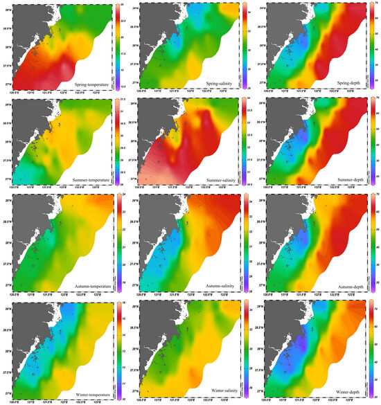
Figure 3.
Average distribution of marine environmental factors in south offshore of Zhejiang in 2018–2019.
3.2. Distribution of Abundance Data of S. taty
From 2018 to 2019, S. taty abundance showed a strongly skewed distribution. Specifically, 24.2% of survey records recorded zero catches (Figure 4). For non-zero values, abundance generally ranged between 0 and 500 ind·km−2, though certain stations reached as high as 2000 ind·km−2, indicating marked overdispersion.
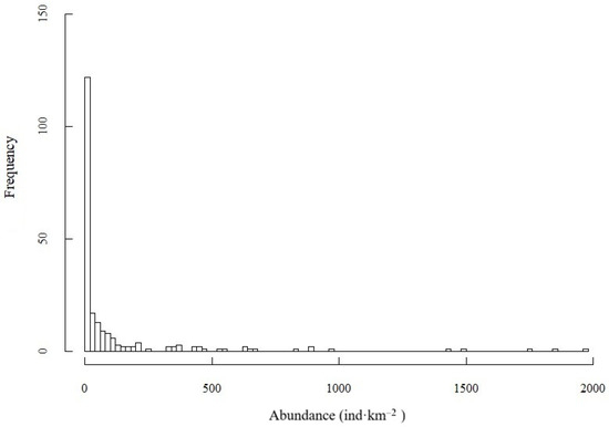
Figure 4.
Frequency distribution of S. taty abundance observations.
3.3. Model Development and Performance Evaluation
3.3.1. Model Selection Result
VIF tests indicated that longitude and latitude had values exceeding 5 (Table 1), suggesting strong multicollinearity and necessitating their removal. The remaining four predictors, temperature, depth, salinity, and season, were included in both ZIP and ZINB models. Results from 1000 cross-validation runs (Table 2) demonstrated that ZINB had superior predictive performance (RMSE = 199.1, R2 = 0.25) compared to ZIP (RMSE = 239.4, R2 = 0.23). Consequently, we selected ZINB for subsequent analyses. Based on smallest AIC value, the combination of “temperature + depth + season” on both sides of the zero-inflation separator yielded the best model fit (Table 3), and was thus retained in the final model.
Table 2.
Parameter results of cross-validation of ZINB and ZIP.
Table 3.
AIC value of the combination of environmental factors on the left and right sides of ZINB.
3.3.2. Final Model Performance
The final ZINB model exhibited acceptable fit and predictive accuracy, mitigating biases associated with zero inflation and overdispersion. The outcomes of the different combination of environmental factors confirm that temperature, depth, and season together exert a significant influence on S. taty abundance.
3.4. Analysis of Response Curves of Environmental Factors
Analyses of temperature, salinity, and depth across the four seasons of 2018–2019 (Figure 5) revealed clear seasonal responses in S. taty abundance. In winter (10.4–15.8 °C), abundance declined with rising temperature but peaked around 11–12 °C. In spring (12.5–25 °C), abundance increased with temperature, peaking at approximately 19–20 °C. Summer (28–34 °C) followed a similar pattern, with elevated abundance near 34 °C. In contrast, autumn (19–24 °C) showed decreasing abundance as temperature rose, concentrating around 19 °C.
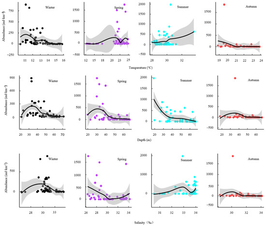
Figure 5.
ZINB model response curves showing seasonal effects of temperature, depth, and salinity on S. taty abundance (2018–2019). Points are observed station values; solid lines are model predicted mean abundance as the focal variable varies with other covariates held constant; the shadow shows 95% confidence intervals.
Depth also influenced abundance. Winter, spring, and autumn catches were generally higher between 30 and 40 m, whereas summer catches peaked near 20 m. Salinity preferences were season-specific. Highest abundances occurred at approximately 30 psu in winter, 26–28 psu in spring, and peaked at 33–34 psu in summer, while autumn abundance peaked between 29–31 psu.
3.5. Prediction of Spatio-Temporal Distribution of S. taty Abundance
Using environmental data from 2020, the final ZINB model predicted S. taty abundance for spring, summer, and autumn (Figure 6). Among these seasons, summer was projected to have the highest overall abundance, followed by spring and then autumn. Spatially, abundance decreased with distance from shore, with notable hotspots located west of 122° E. In spring, moderate-to-high abundance was found between 27.5° N and 28.5° N, especially in nearshore waters extending northward to 29° N. During summer, abundance increased substantially, forming a broad high-abundance band from Taizhou to Wenzhou. By autumn, high-abundance areas shifted slightly southward along the Zhejiang coast, while offshore abundances remained low.
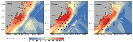
Figure 6.
Distribution of predicted abundance of S. taty in the south offshore of Zhejiang in spring, summer and autumn in 2020. Dots represent observations of S. taty abundance in 2020, with dot size proportional to the observed abundance.
A comparison between predicted and observed values from the 2020 survey stations indicated reasonable agreement (Table 4), with mean bias (predicted−observed) and RMSE of 61.20 and 125.14 in spring, −25.53 and 110.14 in summer, and 45.57 and 60.59 in autumn, respectively; bias was not statistically different from zero in spring and summer (p > 0.05) but was significantly positive in autumn (p = 0.0012).
Table 4.
Seasonal bias and RMSE of ZINB predictions compared with 2020 survey observations.
In addition, a qualitative comparison with the observed spatial patterns from 2018–2019 (Figure 7), suggests that the ZINB model reproduces the main distribution features of S. taty in these offshore waters; notably, the predicted high-abundance areas are relatively similar to the 2018–2019 observations, with higher abundance concentrated in coastal nearshore and southern waters, supporting the interpretation that the model captures the key environmental drivers of abundance.
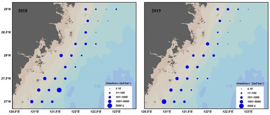
Figure 7.
Distribution of S. taty in the south offshore of Zhejiang in 2018–2019.
4. Discussion
4.1. Why Zero-Inflated Models Are Needed for Fishery Monitoring Data
Fishery monitoring data, including those for S. taty in this study, often contain a high proportion of zero observations. This zero-inflation phenomenon arises from various factors such as inherent limitations of survey design, environmental heterogeneity in sampling areas, seasonal appearance and migration patterns of target species, and the selectivity and efficiency of fishing gear [10,27]. When the proportion of zero counts is very large, traditional count models (for example, Poisson regression or standard negative binomial regression) frequently fail to fit the data adequately, leading to considerable discrepancies between model predictions and observed outcomes [15,35,36]. Poisson regression assumes that the conditional variance equals the conditional mean, and although standard negative binomial regression accounts for overdispersion (variance exceeding the mean), neither approach effectively differentiates “structural zeros” from “sampling zeros” when zeros are highly prevalent, which can result in estimation bias [36,37].
4.2. Comparing ZINB and ZIP in Modeling Zero-Inflated Fishery Data
To address this issue, we considered two commonly used zero-inflated models: the (ZIP model and the ZINB model. Both models conceptualize the data-generation process in two stages. The first stage, often called the zero-inflation component (modeled using a logit or probit function), estimates the probability of structural zeros, which indicate the true absence of fish due to completely unsuitable habitats or genuine absence in a given spatiotemporal context [18,38]. The second stage uses a negative binomial distribution to model sampling zeros (cases where fish are present but not caught) together with positive counts. The key distinction between ZIP and ZINB lies in the assumed distribution for the count component. ZIP uses a Poisson distribution, which retains the Poisson mean–variance relationship in the count process. Consequently, ZIP is most appropriate when excess zeros are the primary deviation from a standard Poisson model and when overdispersion in the positive counts is limited. In contrast, ZINB uses a negative binomial distribution for the count component, allowing additional variability beyond the Poisson assumption and providing greater flexibility when overdispersion is present [15]. This two-part ZINB structure can therefore accommodate both zero inflation and extra-Poisson variation, offering a more realistic framework for fishery abundance data that commonly exhibit abundant zeros and heterogeneous count variability [35].
In this study, the zero-catch rate for S. taty was 24.2%, and the data exhibited significant overdispersion. According to Xu et al. [39], when the proportion of zeros exceeds 60%, ZINB generally outperforms ZIP, because ZIP’s Poisson component still assumes that the conditional mean equals the conditional variance [37], a requirement that is often violated in fishery data. Based on these data characteristics and model selection criteria, the ZINB model was identified as the most appropriate analytical tool for characterizing S. taty abundance patterns under diverse environmental conditions. This choice aligns with a growing trend in fishery ecology toward approaches that robustly accommodate zero-inflated data. For instance, Ma et al. [27] analyzed Engraulis japonicus in the offshore waters of southern Zhejiang using several models, including the Tweedie-generalized additive model (GAM), generalized additive mixed models, and two-stage GAM. They found that two-stage GAMs, which separately model presence/absence and abundance, performed best when confronted with large zero proportions. This conclusion is highly consistent with the core principle of the two-stage ZINB framework in the present study, which separately models zero-generation and count processes. Although two-stage generalized additive models and ZINB differ in their technical implementation [35,40], both approaches emphasize the importance of properly handling zero-inflation and identifying key environmental drivers. These comparisons not only underscore the stableness of our findings but also highlight ZINB’s potential for providing reliable ecological insights, especially when dealing with data sets characterized by complex zero structures.
4.3. Key Environmental Factors and the Spatiotemporal Distribution of S. taty
This study indicates that the spatiotemporal distribution patterns of S. taty in the offshore waters of southern Zhejiang are significantly influenced by key environmental variables. Based on the preliminary screening of the model using AIC values, salinity exerted a weaker effect on the occurrence of S. taty and was therefore excluded from the zero-inflation component of the final model. Ultimately, temperature, water depth, and season were identified as critical environmental factors influencing the non-zero occurrence of S. taty. In the second stage of the count model (negative binomial part), temperature, water depth, and season were again retained as important variables explaining S. taty abundance. These findings suggest that these three factors are the primary environmental drivers of S. taty distribution in the offshore waters of southern Zhejiang and that they intersect closely with the species’ life-cycle activities, including seasonal migration, spawning, and foraging.
As a typical warm-temperate migratory fish, S. taty exhibits high sensitivity to temperature fluctuations [41]. Temperature directly affects metabolic rate, feeding activity, and reproductive rhythms, and it is a core determinant of both the geographical range and seasonal migration of S. taty [10]. In the present study, a higher abundance was observed during winter at temperatures of 11–12 °C, consistent with the suitable temperature range of 10–12 °C identified in the northern East China Sea [6]. In spring, the abundance peak occurred at approximately 19–20 °C, which aligns well with observations made by Zhang et al. [42] in the southern Bohai Sea, where a suitable temperature range of 16–20 °C was recorded in May. The autumn data suggest that S. taty prefers a relatively lower temperature of around 19 °C, probably due to the physiological need to store energy for overwintering [43]. During this period, fish actively accumulate glycogen and other reserves that enhance their survival in low-temperature conditions. At the same time, lower temperatures help reduce metabolic rates, allowing fish to rely on stored resources for an extended period. These seasonal temperature preferences are consistent with the findings of Liu et al. [10], who identified an optimal spring temperature of approximately 21 °C and an optimal autumn temperature of around 18 °C for S. taty in the offshore waters of southern Zhejiang. Han et al. [44] further emphasized the dominant role of temperature in the interannual variation of S. taty in the Yellow Sea, highlighting temperature as a central driver of its distribution. Taken together, these findings strongly support the classic migration theory that S. taty moves from its overwintering grounds to coastal spawning areas in spring as water temperatures rise [45].
Water depth is also an important physical factor affecting the distribution of S. taty. It modifies habitat suitability by changing water temperature, light intensity, and pressure [46]. The results of this study show that the abundance of S. taty is significantly higher at depths of 30–40 m, which parallels previous observations in the northern East China Sea at 28–40 m [6] and in the southern Yellow Sea at 15–35 m [47]. These findings indicate that S. taty tends to inhabit nutrient-rich shelf waters of moderate depth. However, the results differ from the optimal depth of around 20 m proposed by Liu et al. [10], possibly because the seasonal modeling approach in this study places greater emphasis on seasonal effects on depth preference, and because the modeling method differs from that employed in other work. In particular, the preference of S. taty for coastal shelf waters at moderate depths during specific seasons suggests that implementing seasonal or depth specific fishing restrictions could effectively protect critical habitats and ensure stock recruitment.
In addition, the model predictions of S. taty distribution hotspots closely match actual catch data, confirming that S. taty prefers coastal waters. These waters often receive substantial inputs of inorganic nitrogen and other nutrients from rivers and human activities, significantly enhancing primary productivity and providing abundant food sources for fish to aggregate [48]. Furthermore, when the southwest monsoon prevails, coastal upwelling frequently occurs in the southern Zhejiang region, bringing nutrient-rich subsurface water to the surface and increasing chlorophyll a concentration. This stimulates phytoplankton blooms, and supports a high abundance of zooplankton, which in turn attract many migratory fishes, including S. taty, to forage and aggregate [13,49].
Although the final model identified physical drivers, additional mechanisms may further shape the observed hotspots, particularly in nearshore waters where nutrient inputs and seasonal upwelling can enhance primary productivity (e.g., higher chlorophyll a), increase zooplankton availability, and promote fish aggregation. Prey availability (e.g., zooplankton biomass) and other biotic interactions (such as predation and competition) may also modulate local abundance and aggregation patterns [50]. Variables such as chlorophyll a [51], turbidity, current velocity and biotic interactions are therefore expected to improve mechanistic interpretation and predictive skill [51]. However, these factors were not incorporated here because they were not measured in the underlying survey program and were unavailable for analysis.
The spatio-temporal predictions generated from the ZINB model provide useful reference information for managing S. taty resources in the southern offshore waters of Zhejiang. The predictions indicate clear seasonal differences (e.g., higher abundance in summer) and identify high-density areas in coastal waters off Wenzhou and Taizhou west of 122° E. These outputs can help prioritize areas for monitoring and field verification, and can support subsequent evaluation of spatial management options, such as zoning and seasonal effort regulation. Any management actions, however, should align with management objectives and be updated as new data become available.
5. Conclusions
- Using a zero-inflated modeling framework, this study characterized the spatio-temporal distribution of S. taty in the southern offshore waters of Zhejiang, China, and identified temperature, water depth, and season as the main predictors associated with its variability.
- The observed zero proportion exceeded that expected under baseline count models (0.26% under Poisson; 24.24% under negative binomial), and the Poisson dispersion ratio (Pearson χ2/df) was ≈293, indicating strong overdispersion. These diagnostics justify the use of ZINB as an appropriate final model for prediction and interpretation.
- S. taty abundance showed clear seasonal thermal associations, with higher abundance at 11–12 °C in winter, peaking at 19–20 °C in spring, and remaining relatively higher around 19 °C in autumn; abundance was also highest at 30–40 m depth. Seasonal predictions for spring–autumn 2020 indicated a summer peak, a nearshore-to-offshore decreasing gradient, and a nearshore hotspot off Wenzhou and Taizhou west of 122° E.
- These spatially explicit outputs provide reference information for regional monitoring and resource management. Future work could improve predictive skill and ecological realism by integrating additional environmental indicators (e.g., chlorophyll a, current velocity) and biotic information (e.g., prey availability) when available, extending spatio-temporal monitoring, and comparing alternative zero-inflated models under different data conditions.
Author Contributions
Conceptualization, methodology and writing—original manuscript preparation, X.L.; conceptualization and suggestion, W.M.; drafting guidance, J.M.; manuscript preparation, C.G.; drawing guidance, W.C.; data curation, supervision and funding acquisition, J.Z. All authors have read and agreed to the published version of the manuscript.
Funding
This work was funded by the National Natural Science Foundation of China (Grant No. 31902372) and Zhejiang Mariculture Research Institute of China (Project No. 325000).
Institutional Review Board Statement
Not applicable.
Data Availability Statement
The data presented in this study are available on request from the author. The data are not publicly available due to privacy. Images employed for the study will be available online for readers.
Acknowledgments
The authors would like to thank teachers and students from the Laboratory of Quantitative Assessment and Management of Fishery Resources and Ecosystems, Shanghai Ocean University and the Zhejiang Mariculture Research Institute, China, for their help in sample collection and biological analysis.
Conflicts of Interest
The authors declare no conflicts of interest.
References
- Kirby, R.R.; Beaugrand, G.; Lindley, J.A. Synergistic effects of climate and fishing in a marine ecosystem. Ecosystems 2009, 12, 548–561. [Google Scholar] [CrossRef]
- Wang, J.; Gao, C.; Tian, S.; Han, D.; Ma, J.; Dai, L.; Ye, S. Shifts in composition and co-occurrence patterns of the fish community in the south inshore of Zhejiang, China. Glob. Ecol. Conserv. 2023, 44, e02502. [Google Scholar] [CrossRef]
- Pauly, D.; Christensen, V.; Dalsgaard, J.; Froese, R.; Torres, F. Fishing down marine food webs. Science 1998, 279, 860–863. [Google Scholar] [CrossRef]
- Liu, Y.; Cheng, J.; Chen, X. Studies on the seasonal distribution of Setipinna taty in the East China Sea. Mar. Fish. Res. 2006, 27, 1–6. [Google Scholar]
- Han, Q.; Shan, X.; Jin, X.; Gorfine, H.; Yang, T.; Su, C. Data-limited stock assessment for fish species devoid of catch statistics: Case studies for pampus argenteus and Setipinna taty in the bohai and yellow seas. Front. Mar. Sci. 2021, 8, 766499. [Google Scholar] [CrossRef]
- Liu, Y.; Cheng, J.; Li, S. A study on the distribution of Setipinna taty in the East China Sea. Mar. Fish. 2004, 26, 255–260. [Google Scholar]
- Froese, R.; Pauly, D. Setipinna taty (Valenciennes, 1848). FishBase. Available online: https://www.fishbase.se (accessed on 20 September 2025).
- Jin, X.; Cheng, J.; Qiu, S.; Li, P.; Cui, Y.; Dong, J. The General Study and Evaluation of Fisheries Resources in Yellow Sea and Bohai Sea; Ocean Press: Beijing, China, 2006. [Google Scholar]
- Li, H.; Xu, T.; Cheng, Y.; Sun, D.; Wang, R. Genetic diversity of Setipinna taty (Engraulidae) populations from the China Sea based on mitochondrial DNA control region sequences. Genet. Mol. Res. 2012, 11, 1230–1237. [Google Scholar] [CrossRef] [PubMed]
- Liu, X.; Gao, C.; Zhao, J.; Tian, S.; Ye, S.; Ma, J. Modeling and comparison of count data containing zero values: A case study of Setipinna taty in the south inshore of Zhejiang, China. Environ. Sci. Pollut. Res. 2021, 28, 46827–46837. [Google Scholar] [CrossRef]
- Liu, W.; Zhang, T.; Chen, G.; Ye, S.; Gao, C.; Han, D. Feeding habits of Setipinna taty and its relationship with environmental factors in southern coastal waters of Zhejiang, China. Chin. J. Appl. Ecol. 2024, 35, 3174–3182. [Google Scholar]
- Ma, W.; Ding, L.; Wu, X.; Gao, C.; Ma, J.; Zhao, J. Impacts of data sources on the predictive performance of species distribution models: A case study for Scomber japonicus in the offshore waters southern Zhejiang, China. Acta Oceanol. Sin. 2025, 43, 113–122. [Google Scholar] [CrossRef]
- Liu, X.; Gao, C.; Tian, S.; Qin, S.; Ma, J.; Zhao, J. Distribution of optimal habitat for Setipinna taty in the southern coastal waters of Zhejiang based on habitat suitability index. J. Fish. Sci. China 2020, 27, 1485–1495. [Google Scholar]
- Chen, X.J. Fishery Resources and Fisheries, 2nd ed.; Ocean Press: Beijing, China, 2014; pp. 152–167. [Google Scholar]
- Arab, A.; Holan, S.H.; Wikle, C.K.; Wildhaber, M.L. Semiparametric bivariate zero-inflated poisson models with application to studies of abundance for multiple species. Environmetrics 2012, 23, 183–196. [Google Scholar] [CrossRef]
- Ma, J.; Li, B.; Zhao, J.; Wang, X.; Hodgdon, C.T.; Tian, S. Environmental influences on the spatio-temporal distribution of Coilia nasus in the Yangtze River estuary. J. Appl. Ichthyol. 2020, 36, 315–325. [Google Scholar] [CrossRef]
- Yau, K.K.W.; Wang, K.; Lee, A.H. Zero-inflated negative binomial mixed regression modeling of over-dispersed count data with extra zeros. Biometrical J. 2003, 45, 437–452. [Google Scholar] [CrossRef]
- Zhao, J.; Liu, X.; Wu, J.; Han, D.; Tian, S.; Ma, J. Application of zero-inflated model in predicting the distribution of rare fish species: A case study of Coilia nasus in Yangtze estuary. Chin. J. Ecol. 2020, 39, 3155–3163. [Google Scholar]
- Zeng, P.; Liu, G.; Cao, H. Application of zero-inflated models in study of the impacting factors about segment number of myocardial ischemia. Chin. J. Health Stat. 2008, 25, 464–466. [Google Scholar]
- Zuur, A.F.; Ieno, E.N.; Walker, N.J.; Saveliev, A.A.; Smith, G.M. Mixed effects models and extensions in ecology with R. Technometrics 2010, 52, 464–465. [Google Scholar]
- Lynch, D.R.; McGillicuddy, D.J.; Werner, F.E. Skill assessment for coupled biological/physical models of marine systems preface. J. Mar. Syst. 2009, 76, 4–15. [Google Scholar] [CrossRef]
- Haslett, J.; Parnell, A.C.; Hinde, J.; de Andrade Moral, R. Modelling excess zeros in count data: A new perspective on modelling approaches. Int. Stat. Rev. 2022, 90, 216–236. [Google Scholar] [CrossRef]
- Jung, B.C.; Jhun, M.; Lee, J.W. Bootstrap tests for overdispersion in a zero-inflated poisson regression model. Biometrics 2005, 61, 626–628. [Google Scholar] [CrossRef]
- Minami, M.; Lennert-Cody, C.E.; Gao, W.; Roman-Verdesoto, M. Modeling shark bycatch: The zero-inflated negative binomial regression model with smoothing. Fish Res. 2007, 84, 210–221. [Google Scholar] [CrossRef]
- Virgili, A.; Racine, M.; Authier, M.; Monestiez, P.; Ridoux, V. Comparison of habitat models for scarcely detected species. Ecol. Model. 2017, 346, 88–98. [Google Scholar] [CrossRef]
- Wang, Y.; Jiang, G.; Dong, H. Distribution characteristics and relationship of dissolved oxygen, pH value and nutrients in the southern sea of Zhejiang in spring. Acta. Oceanol. Sin. 1990, 12, 654–660. [Google Scholar]
- Ma, W.; Gao, C.; Tang, W.; Qin, S.; Ma, J.; Zhao, J. Relationship between Engraulis japonicus resources and environmental factors based on multi-model comparison in offshore waters of southern Zhejiang, China. J. Mar. Sci. Eng. 2022, 10, 657. [Google Scholar] [CrossRef]
- Standard No. GB/T 12763.6–2007; Specifications for Oceanographic Survey—Part 6: Marine Biological Survey. China Standards Press: Beijing, China, 2007.
- Standard No. GB 17378.3–1998; The Specification for Marine Monitoring—Part 3: Sample Collection, Storage and Transportation. China Standards Press: Beijing, China, 1998.
- Marcoulides, K.M.; Raykov, T. Evaluation of variance inflation factors in regression models using latent variable modeling methods. Educ. Psychol. Meas. 2019, 79, 874–882. [Google Scholar] [CrossRef]
- Sosebee, K.A.; Musick, J.A.; Rago, P.J.; Cerrato, R.M. Application of generalized additive models to examine ontogenetic and seasonal distributions of spiny dogfish (Squalus acanthias) in the northeast (US) shelf large marine ecosystem. Can. J. Fish. Aquat. Sci. 2014, 71, 847–877. [Google Scholar] [CrossRef]
- Chang, J.-H.; Chen, Y.; Holland, D.; Grabowski, J. Estimating spatial distribution of American lobster Homarus americanus using habitat variables. Mar. Ecol.-Prog. Ser. 2010, 420, 145–156. [Google Scholar] [CrossRef]
- Planque, B.; Bellier, E.; Lazure, P. Modelling potential spawning habitat of sardine (Sardina pilchardus) and anchovy (Engraulis encrasicolus) in the Bay of Biscay. Fish Oceanogr. 2007, 16, 16–30. [Google Scholar] [CrossRef]
- R Core Team. R: A Language and Environment for Statistical Computing; R Foundation for Statistical Computing: Vienna, Austria, 2019. [Google Scholar]
- Zeileis, A.; Kleiber, C.; Jackman, S. Regression Models for Count Data in R. J. Stat. Softw. 2008, 27, 1–25. [Google Scholar] [CrossRef]
- He, H.; Tang, W.; Wang, W.; Crits-Christoph, P. Structural zeroes and zero-inflated models. Shanghai Arch. Psychiatry 2014, 26, 236–242. [Google Scholar] [PubMed]
- Joseph, L.N.; Elkin, C.; Martin, T.G.; Possingham, H.P. Modeling abundance using N-mixture models: The importance of considering ecological mechanisms. Ecol. Appl. 2009, 19, 631–642. [Google Scholar] [CrossRef]
- Dean, C.; Lawless, J. Tests for detecting overdispersion in poisson regression-models. J. Am. Stat. Assoc. 1989, 84, 467–472. [Google Scholar] [CrossRef]
- Perumean-Chaney, S.E.; Morgan, C.; McDowall, D.; Aban, I. Zero-inflated and overdispersed: What’s one to do? J. Stat. Comput. Simul. 2013, 83, 1671–1683. [Google Scholar] [CrossRef]
- Xu, T.; Li, W.; Chen, T. Application of zero-inflated models on regression analysis of count data: A study of sub-health symptoms. Chin. J. Epidemiol. 2011, 32, 187–191. [Google Scholar]
- Li, B.; Cao, J.; Chang, J.; Wilson, C.; Chen, Y. Evaluation of effectiveness of fixed-station sampling for monitoring American lobster settlement. N. Am. J. Fish. Manage. 2015, 35, 942–957. [Google Scholar] [CrossRef]
- Li, Q.; Jiang, R.; Zhao, P.; Zhang, Q.; Liu, M.; Shen, J.; Zhang, H.; Zhu, W.; Long, X. Study on the potential suitable areas of Setipinna taty in Zhejiang coastal sea area based on MaxEnt model. J. Fish. Sci. China 2025, 32, 93–102. [Google Scholar]
- Zhang, M.; Sun, T.; Li, Y.; Wang, X.; Guo, J. On seasonal distribution of Setipinna taty in southern Bohai Sea. Shandong Fish. 1995, 12, 10–13. [Google Scholar]
- Piironen, J.; Holopainen, I. A note on seasonality in anoxia tolerance of crucian carp (Carassius carassius (L.)) in the laboratory. Ann. Zool. Fenn. 1986, 23, 335–338. [Google Scholar]
- Han, Q.; Shan, X.; Jin, X.; Gorfine, H.; Jin, Y.; Wu, Q.; Shi, Y. Understanding the effects of climate and anthropogenic stresses on distribution variability of Setipinna taty in the yellow sea. Fish Res. 2024, 276, 107037. [Google Scholar] [CrossRef]
- Li, J.; Zhang, Q.; Zheng, Y.; Hong, W. Review and prospect of biological study on common marine pelagic commercial fishes in China. Mar. Fish. 2014, 36, 565–575. [Google Scholar]
- Ma, W.; Qin, S.; Gao, C.; Tang, W.; Ma, J.; Zhao, J. Distribution of Japanese scad (Decapterus maruadsi) and its relationship with environmental factors in the coast waters of southern Zhejiang based on the Tweedie-GAM. Prog. Fish. Sci. 2023, 44, 12–22. [Google Scholar]
- Li, Z.; Ye, Z.; Zhang, C.; Zhuang, L.; Wang, M. CPUE distribution of Setipinna taty in southern Yellow Sea and its influencing factors revealed by stow net fishing in spring. Period. Ocean Univ. China 2013, 43, 30–36. [Google Scholar]
- Liu, Z.; Yang, L.; Yan, L.; Yuan, X.; Cheng, J. Fish assemblages and environmental interpretation in the northern Taiwan Strait and its adjacent waters in summer. J. Fish. Sci. China 2016, 23, 1399–1416. [Google Scholar]
- Zerbini, A.N.; Friday, N.A.; Palacios, D.M.; Waite, J.M.; Ressler, P.H.; Rone, B.K.; Moore, S.E.; Clapham, P.J. Baleen whale abundance and distribution in relation to environmental variables and prey density in the Eastern Bering Sea. Deep Sea Res. Part II 2016, 134, 312–330. [Google Scholar] [CrossRef]
- Zhang, C.; Shang, S.; Hong, H. Spatial patterns of annual cycles in surface chlorophyll a in the Taiwan Strait. Acta Oceanol. Sin. 2006, 28, 165–170. [Google Scholar]


Disclaimer/Publisher’s Note: The statements, opinions and data contained in all publications are solely those of the individual author(s) and contributor(s) and not of MDPI and/or the editor(s). MDPI and/or the editor(s) disclaim responsibility for any injury to people or property resulting from any ideas, methods, instructions or products referred to in the content. |
© 2026 by the authors. Licensee MDPI, Basel, Switzerland. This article is an open access article distributed under the terms and conditions of the Creative Commons Attribution (CC BY) license.