Article

Local Spatial Attention Transformer with First-Order Difference for Sea Level Anomaly Field Forecast: A Regional Study in the East China Sea

1
Marine Science and Technology College, Zhejiang Ocean University, Zhoushan 316022, China
2
South China Sea Forecast and Disaster Reduction Center, Ministry of Natural Resources, Guangzhou 510310, China
3
College of Ocean Science and Engineering, Shandong University of Science and Technology, Qingdao 266590, China
*
Authors to whom correspondence should be addressed.
J. Mar. Sci. Eng. 2026, 14(1), 54; https://doi.org/10.3390/jmse14010054 (registering DOI)
Submission received: 30 November 2025 / Revised: 22 December 2025 / Accepted: 26 December 2025 / Published: 28 December 2025
(This article belongs to the Section Ocean Engineering)

Abstract

Accurate prediction of regional sea level anomaly (SLA) is critical for coastal hazard early warning, navigation safety, and infrastructure protection in economically active marginal seas such as the East China Sea (ECS), yet complex multiscale air–sea dynamics still make SLA forecasting challenging. This study proposes a Local Spatial Attention Transformer Network (LSATrans-Net) for short-term regional SLA prediction in the ECS, which incorporates a Local Spatial Attention mechanism designed for regional ocean processes and employs a first-order difference preprocessing strategy to reduce error accumulation induced by data non-stationarity. The LSATrans-Net outperforms ConvLSTM, BiLSTM, and CNN-Transformer in 7-day prediction experiments, with an RMSE of 0.017 m and a PCC of 0.984, with particularly strong forecasting skill in the ECS-Kuroshio and eddy-active regions. LSATrans-Net provides an efficient and physically interpretable framework for high-precision short-term SLA forecasting in dynamically complex marine regions, and offers reliable technical support for coastal disaster prevention and operational ocean forecasting systems.

1. Introduction

Sea level anomaly (SLA) is an essential parameter for monitoring sea level variability and supporting marine disaster early-warning systems [1,2]. Variations in SLA exert significant influences on global and regional climate change and extreme weather events [3,4]. An accurately predicting SLA is not only crucial for monitoring and assessing global and regional marine environments, but also essential for ensuring maritime safety and the stable operation of ocean engineering.
The East China Sea (ECS) is a vast marginal sea, bordered by the Northwest Pacific to the east, adjoined by the Yellow Sea to the north, and connected to the Taiwan Strait to the south, with its water depth gradually increasing from northwest to southeast [5]. The dynamic system of the ECS is highly complex and is influenced by multiple factors, including tides, monsoons, coastal currents along the mainland, the Kuroshio Current, and discharge from the Yangtze River [6]. The coastal region of ECS has dense populations and concentrated economic activities, making it particularly vulnerable to sea-level fluctuations [7,8]. Over the past two decades, the mean sea-level rise rate in the ECS has exceeded the global average. This acceleration, combined with the frequent occurrence of extreme events such as storm surges, has significantly increased the risk of coastal flooding in urbanized areas [6,9,10]. Developing an accurate regional SLA prediction model for the ECS is beneficial for making climate adaptation strategies and implementing coastal disaster prevention and mitigation measures.
Methods for predicting SLA can be divided into two major categories, which include physics-based numerical modeling and data-driven modeling. Physics-based numerical models simulate and forecast sea-level variations by solving complex equations that describe ocean dynamics [11,12,13]. Although grounded in theory and high physical interpretability, numerical models are highly sensitive to initial and boundary conditions, and they face huge computational costs for high-resolution simulations. In contrast, data-driven models offer superior flexibility and generalizability for modeling complex marine systems by directly capturing nonlinear spatiotemporal relationships from observational data, without the need for equation solving or the high computational costs of physical models.
Data-driven models for sea-level prediction can be broadly classified into traditional statistical methods and deep learning methods. Conventional statistical methods, such as the Autoregressive Integrated Moving Average (ARIMA) [14], the Markov model [15], and Canonical Correlation Analysis (CCA) [16], are simple and computationally efficient, and can capture certain temporal patterns. However, their prediction accuracy is limited by the inadequate representation of nonlinear dynamics and spatial structures. Deep learning methods, such as Recurrent Neural Networks (RNN) [17,18] and Long Short-Term Memory networks (LSTM) [19,20,21], have been widely used for time-series prediction. The Convolutional LSTM (ConvLSTM) incorporates convolutional operations, enabling the simultaneous modeling of spatial and temporal features [22,23,24], which enhances performance on complex spatiotemporal data. However, these recurrent models can still suffer from issues such as vanishing or exploding gradients when handling long sequences, limiting their ability to capture long-term dependencies [25]. Additionally, their sequential processing nature hinders parallelization, reducing efficiency and scalability for large-scale forecasting tasks [26].
Recently, Transformer architectures based on self-attention have shown outstanding performance in sequence prediction by effectively capturing long-range spatiotemporal dependencies [27]. Transformers have been increasingly applied in oceanographic forecasting [28,29]. However, despite their effectiveness in forecasting oceanic variables, the application of Transformers to SLA prediction requires further exploration. This is because SLA exhibits strong local spatial heterogeneity, which is incompatible with the Transformer’s self-attention mechanism. This mechanism is primarily designed to capture global patterns by weighting all points, thereby failing to account for distance-decaying autocorrelation [30].
This study proposes a Local Spatial Attention Transformer Network (LSATrans-Net), a hybrid CNN-Transformer model that combines CNN’s ability to capture local spatial features with the Transformer’s strength in modeling dependencies. CNNs effectively extract spatial structures while reducing noise [31], and the Local Spatial Attention mechanism restricts attention to each grid point’s neighborhood rather than all global positions, enabling the model to capture local spatial features of SLA with improved interpretability and performance. To further enhance modeling effectiveness, a distinct data preprocessing strategy is adopted. Because SLA time series are nonlinear and non-stationary, directly using raw SLA data can lead to signal aliasing, obscure long-term trends, and hinder the detection of local anomalies. Although previous studies have addressed these issues using signal decomposition methods such as wavelet decomposition [32], variational mode decomposition (VMD) [33], and empirical orthogonal function (EOF) [34], these approaches often require complex parameter tuning, rely on strong assumptions, and may introduce computational artifacts. Instead, this study applies a first-order differencing method to transform SLA into ΔSLA, a simpler and more efficient preprocessing strategy that has been validated in predictions of significant wave height [35] and regional sea-level rise [36]. Therefore, the proposed LSA-Trans-Net integrates multi-scale feature fusion, a Local Spatial Attention mechanism, and ΔSLA-based input processing to enhance short-term SLA forecasting accuracy.
The remainder of this paper is structured as follows. Section 2 introduces the study area, datasets, and data preprocessing methods. Section 3 introduces the LSATrans-Net model and related contents, along with the compared models and evaluation metrics. Section 4 evaluates the LSATrans-Net model, verifies its robustness and the effectiveness of the ΔSLA strategy, and Section 5 concludes with key findings and remarks.

2. Study Area and Data

2.1. Study Area

In this study, we focus on predicting sea level anomalies in the East China Sea (ECS). As shown in Figure 1, part of the ECS is designated as the study area, geographically delimited by the coordinates 24° N–36° N and 118° E–132° E. The regional bathymetry, depicted by shaded contours in Figure 1, is dominated by an extensive continental shelf where water depths are predominantly less than 200 m. The complex hydrography is governed by several major ocean currents, which are represented by colored arrows. They mainly include the warm currents—namely the Kuroshio Current (KC), Tsushima Warm Current (TWC), Taiwan Warm Current (TWWC), and Yellow Sea Warm Current (YSWC), denoted in red—and the cold coastal currents, including the Subei Coastal Current (SCC) and the Zhe-Min Coastal Current (ZMCC, Zhe represents Zhejiang, Min represents Fujian), denoted in blue. Additionally, the Yangtze River Estuary (YRE), situated between Jiangsu and Zhejiang provinces, has a significant impact on the regional hydrodynamic environment.

2.2. Satellite Altimetry Dataset

The SLA data employed in this study were sourced from the Copernicus Marine Environment Monitoring Service (CMEMS). This dataset is a multi-mission gridded product that combines sea level observations from a constellation of satellite altimeters, including ERS-1/2, Topex/Poseidon, ENVISAT, and the Jason series [37]. It provides daily gridded fields at a native spatial resolution of 1/8° × 1/8°, with a temporal coverage extending from 1 January 1993 to the present. The high spatiotemporal consistency and observational continuity of this product furnish the long-term, stable training samples requisite for deep learning models. To mitigate computational overhead and ensure the feasibility of model training, the native 1/8° resolution data were resampled to a 1/4° × 1/4° grid via bilinear interpolation.
For the purpose of robust model development and objective performance evaluation, the dataset spanning 28 years from 1993 to 2020 was partitioned chronologically into three distinct subsets. The period from January 1993 to December 2015 was allocated for the training set, January 2016 to December 2019 for the validation set, and the entirety of 2020 was reserved for the test set.

2.3. Data Processing

The raw SLA time series exhibits strong long-term trends and Periodic variation, making it a typical non-stationary process that complicates direct modeling. To address this issue, this study applies a first-order differencing preprocessing step, transforming the raw SLA into a ΔSLA sequence that represents changes between consecutive time steps as follows.
Δ S L A t , i , j = S L A t , i , j S L A t 1 , i , j
in which, t denotes the temporal index, while i and j correspond to the spatial grid indices.
Since the model outputs the differenced sequence (ΔSLA), the physically meaningful SLA must be reconstructed for evaluation. This inverse differencing is performed by cumulatively summing the predicted ΔSLA values, initialized with the ground-truth SLA at the forecast start, as expressed as follows.
S L A p r e d t + k = S L A i n i t t + d = 1 k Δ S L A p r e d t + d
in which, S L A i n i t ( t ) is the ground-truth SLA observation at the forecast start time t, Δ S L A p r e d ( t + d ) denotes the model’s predicted difference for the d-th future time step, and S L A p r e t + k is the final reconstructed SLA forecast for the k-th future time step.

3. Method

3.1. LSATrans-Net Model

Section 3.1.1 provides an overview of the LSATrans-Net architecture, followed by a detailed description of the internal data flow and the design of each module. Section 3.1.2 focuses on the Local Spatial Attention mechanism, while Section 3.1.3 presents the detailed hyperparameters and training settings of the model.

3.1.1. Architecture of LSATrans-Net Model

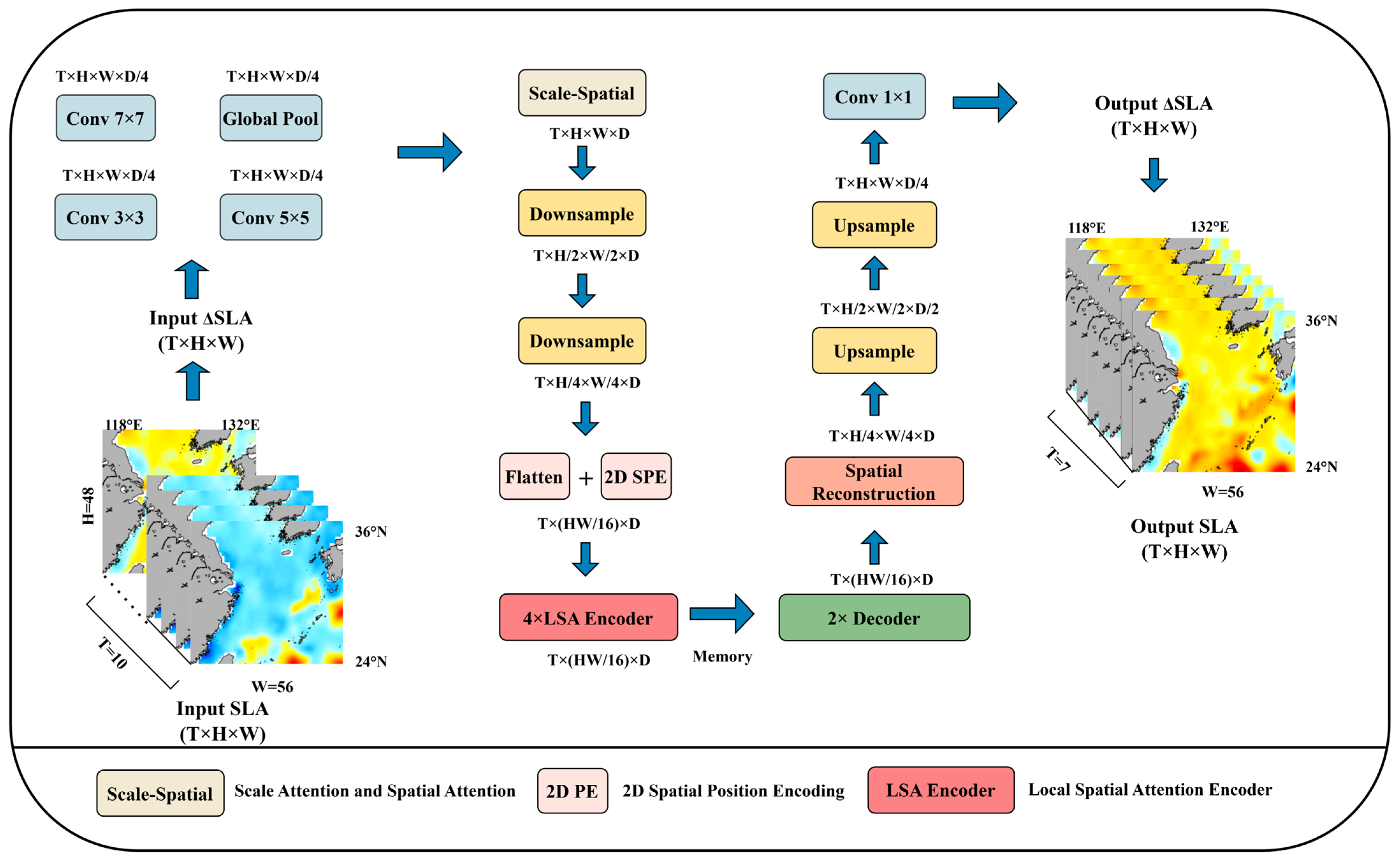
The overall architecture of the LSATrans-Net is shown in Figure 2. The SLA sequence is first preprocessed into ΔSLA to reduce non-stationarity and long-term trends. A multi-scale CNN module then extracts and fuses spatial features across different receptive fields, followed by Local Spatial Attention in the encoder–decoder framework to generate future sequences. Finally, the predicted ΔSLA is reconstructed to obtain the SLA forecasts. Figure 3 illustrates the internal data flow and module design of LSA-Trans-Net, with each component described below.
The model input consists of a 10-day SLA observation sequence. I n p u t R T × H × W , where T = 10 denotes the input time steps, and H × W specifies the spatial resolution (H = 48, W = 56). The input SLA sequence is processed by a first-order differencing operation to obtain the ΔSLA sequence. The ΔSLA sequence is first processed by a multi-scale CNN module with four parallel branches using 3 × 3, 5 × 5, and 7 × 7 convolutions, plus global average pooling, to capture spatial patterns at different scales. Features are adaptively fused using a dual attention mechanism. Scale Attention emphasizes the most informative scales, and Spatial Attention weighs different locations to enhance spatial representation. The fused feature map (D = 256) is downsampled to H/4 × W/4 and then flattened into a 1D feature sequence. A 2D spatial positional encoding (2D SPE) is added to retain each feature vector’s original grid location.
Next, the 1D feature sequence is fed into the encoder, where the Local Spatial Attention mechanism restricts attention to local neighborhoods (Section 3.1.2). The encoder captures temporal and spatial dependencies, outputting memory from multiple time steps and locations. The decoder then uses this memory to generate future predictions at H/4 × W/4 resolution.
Finally, the low-resolution features (H/4 × W/4) are upsampled to the original resolution (H × W) using two convolutional upsampling layers, with each step doubling the spatial size and reducing channels. A 1 × 1 convolution then combines the channels into a single ΔSLA, producing seven-day forecasts, which are finally reconstructed into SLA by cumulatively summing ΔSLA.

3.1.2. Local Spatial Attention

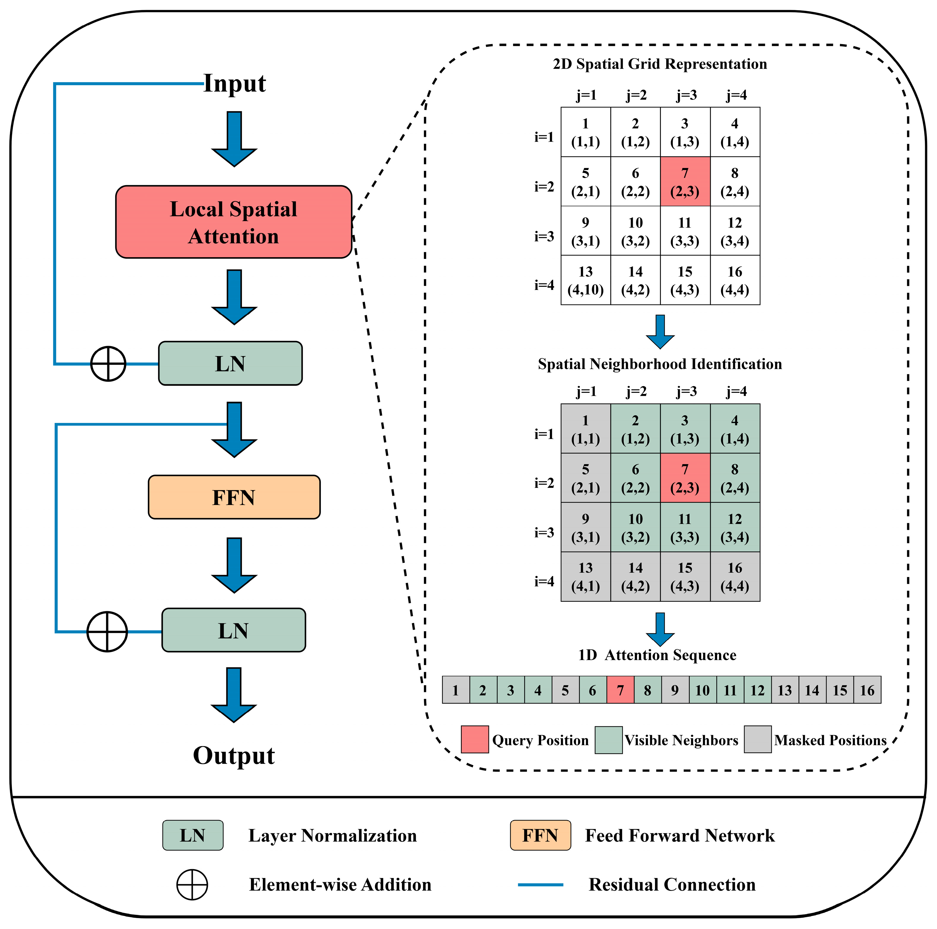
The LSATrans-Net encoder follows the standard Transformer design, with an attention module and feed-forward network (FFN), including residual connections and layer normalization (Figure 4, left). The core innovation of this study is replacing Self-Attention with Local Spatial Attention to better handle local spatial data. In standard Transformers, Self-Attention treats flattened spatial data as an unordered 1D sequence to capture global dependencies, defined as follows.
A t t e n t i o n ( Q , K , V ) = s o f t m a x Q K T d k V
where Q R n × d k , K R n × d k   and   V R n × d v represent the query, key, and value matrices, respectively, and n represents the sequence length; in which d m o d e l denotes the feature dimension of the model, with d k = d v = d m o d e l / h , and h is the number of attention heads.
In studying short-term regional oceanographic variability, local oceanic influences usually outweigh global influences. As shown in Figure 4 (right), it maps the 1D sequence to a 2D grid, identifies spatial neighborhoods, and applies attention locally. Using the 4 × 4 grid in Figure 4 as an example, each position is identified by its spatial coordinate (i, j) and sequence index. For any query, the model defines its spatial neighborhood based on a given radius, as follows.
Spatial   Neighborhood i , j = { m , n : i m r   and   j n r
Here, (i, j) are the query’s row and column coordinates, (m, n) are a candidate neighbor’s coordinates, and r is the spatial radius. As illustrated in Figure 4, for query position (2, 3) with r = 1, all positions within its 3 × 3 neighborhood are identified as neighbors. Based on this, a spatial mask matrix is constructed as follows.
M s p a t i a l i , j , m , n = 0 , if   max ( | i m | , | j n | ) r , else
in this matrix, all positions within the spatial neighborhood are assigned 0, while those outside (marked in gray in Figure 4) are assigned −∞. Local Spatial Attention is formulated as follows.
Local   Spatial   Attention Q , K , V = s o f t m a x M s p a t i a l + Q K T d k V
This mechanism uses the mask matrix to constrain attention locally: positions within the neighborhood keep their scores, while positions outside are set to −∞. After softmax normalization, attention weights outside the neighborhood become zero, ensuring each query focuses only on its spatial neighborhood. As shown in the “1D Attention Sequence” of Figure 4, position 7 (red) considers all 16 positions under Self-Attention, while Local Spatial Attention interacts only with neighboring positions (green), with distant positions (gray) set to zero. In this way, the model can better capture local dependencies, improve predictive performance, and keep the predictions consistent with the spatial characteristics of SLA.

3.1.3. Experimental Implementation Details

The LSATrans-Net model was trained using the hyperparameters and settings in Table 1 on data spanning 1993–2020. The model input/output dimensions are [1, 10, 48, 56] (10-time steps) and [1, 7, 48, 56] (7-step forecast), respectively. The feature dimension of the model is set to 256, which determines the dimensionality of the feature embeddings. The architecture uses 4 attention heads, 4 encoder layers, and 2 decoder layers to balance representational capacity and computational efficiency. A dropout rate of 0.1 is applied to prevent overfitting. The spatial radius is set to 1, enabling Local Spatial Attention within a 3 × 3 neighborhood. Attention is computed on a downsampled 12 × 14 grid (from the original 48 × 56 grid), where each grid cell represents a 1° × 1° resolution, corresponding to an effective range of approximately ±100 km. The choice of this spatial scale is physically motivated by the dominant physical processes influencing SLA variability in the ECS. For instance, the Kuroshio is the most prominent western boundary current in the region. Averaged along its entire path, the Kuroshio exhibits its widest extent (~218 km) in winter and its narrowest (~207 km) in summer, with an annual mean width of approximately 210 km [38]. Statistical analyses based on satellite altimetry further indicate that approximately 82% of detected mesoscale eddies have radii between 30 and 80 km [39]. In addition, the radius of maximum wind (RMW) of typhoons in the northwestern Pacific typically ranges from approximately 30 to 40 km and rarely exceeds 100 km, consistent with statistical analyses of best-track observations and documented inner-core wind structures of intense tropical cyclones [40]. Therefore, the selected local radius r = 1, approximately equivalent to a radius of 100 km or a diameter of 200 km, effectively contains the main physical processes affecting sea level changes. This ensures that the Local Spatial Attention mechanism focuses on the most dynamically relevant spatial correlations. A sensitivity analysis of different spatial radii (r = 1, 3, 5) was conducted to validate this selection, confirming that r = 1 yields optimal predictive performance (see Appendix A for details).
The model was trained for a maximum of 100 epochs with a batch size of 16 and an initial learning rate of 5 × 10⁻⁵. A ReduceLROnPlateau scheduler is used to dynamically adjust the learning rate, reducing it to 70% of its current value if the validation loss does not improve for six consecutive epochs, with a minimum threshold of 1 × 10⁻⁶. An early stopping strategy is also applied, terminating training if the validation loss fails to improve for 10 consecutive epochs and restoring the best-performing model weights.

3.2. Compared Models

To evaluate the performance of LSATrans-Net, three comparison models were selected:
(1)
ConvLSTM: A spatiotemporal model that combines CNN and LSTM by applying convolution operations to both inputs and hidden states, enabling the extraction of spatial features and learning of complex spatiotemporal dependencies.
(2)
BiLSTM: This model consists of two LSTM layers operating in opposite directions, one from past to future and the other from future to past. The architecture combines the benefits of sequential data handling and the long-term memory capacity of forward and backward LSTM [41].
(3)
CNN-Transformer: This model combines CNN and Transformer, employing the same multi-scale CNN module as LSATrans-Net. However, the encoder uses the self-attention mechanism, which computes attention across all spatial positions. Therefore, the CNN-Transformer serves as a direct baseline for evaluating the Local Spatial Attention mechanism of LSATrans-Net.

3.3. Evaluation Metrics

To evaluate model performance, three metrics are used from two perspectives: prediction accuracy and spatial pattern similarity, including Mean Absolute Error (MAE), Root Mean Square Error (RMSE), and the Pearson Correlation Coefficient (PCC). MAE and RMSE quantify numerical deviations between predicted and observed SLA at each grid point, with RMSE being more sensitive to large errors. Lower MAE and RMSE indicate higher accuracy. To assess spatial pattern consistency beyond numerical errors, PCC measures the spatial correlation between predicted and observed fields, with values closer to 1 indicating stronger spatial agreement and better physical reliability.
The formulas for these metrics are as follows:
M A E = 1 N i = 1 N P i T i
R M S E = 1 N i = 1 N ( P i T i ) 2
P C C = i = 1 N ( P i P ¯ ) ( T i T ¯ ) i = 1 N ( P i P ¯ ) 2 i = 1 N ( T i T ¯ ) 2
Here, P i and T i represent the predicted and observed values at the i-th spatial grid point, N denotes the number of grid points, while P ¯ and T ¯ indicate the spatial mean values of the predicted and observed fields, respectively.

4. Results and Discussion

Here, we first systematically evaluated LSATrans-Net’s performance against multiple baseline models based on prediction tasks, then validated the robustness of our proposed model under both normal and extreme weather conditions. Additionally, we demonstrated the effectiveness of the first-order difference strategy (ΔSLA) under our framework in Section 4.3.

4.1. Model Validation and Comparison

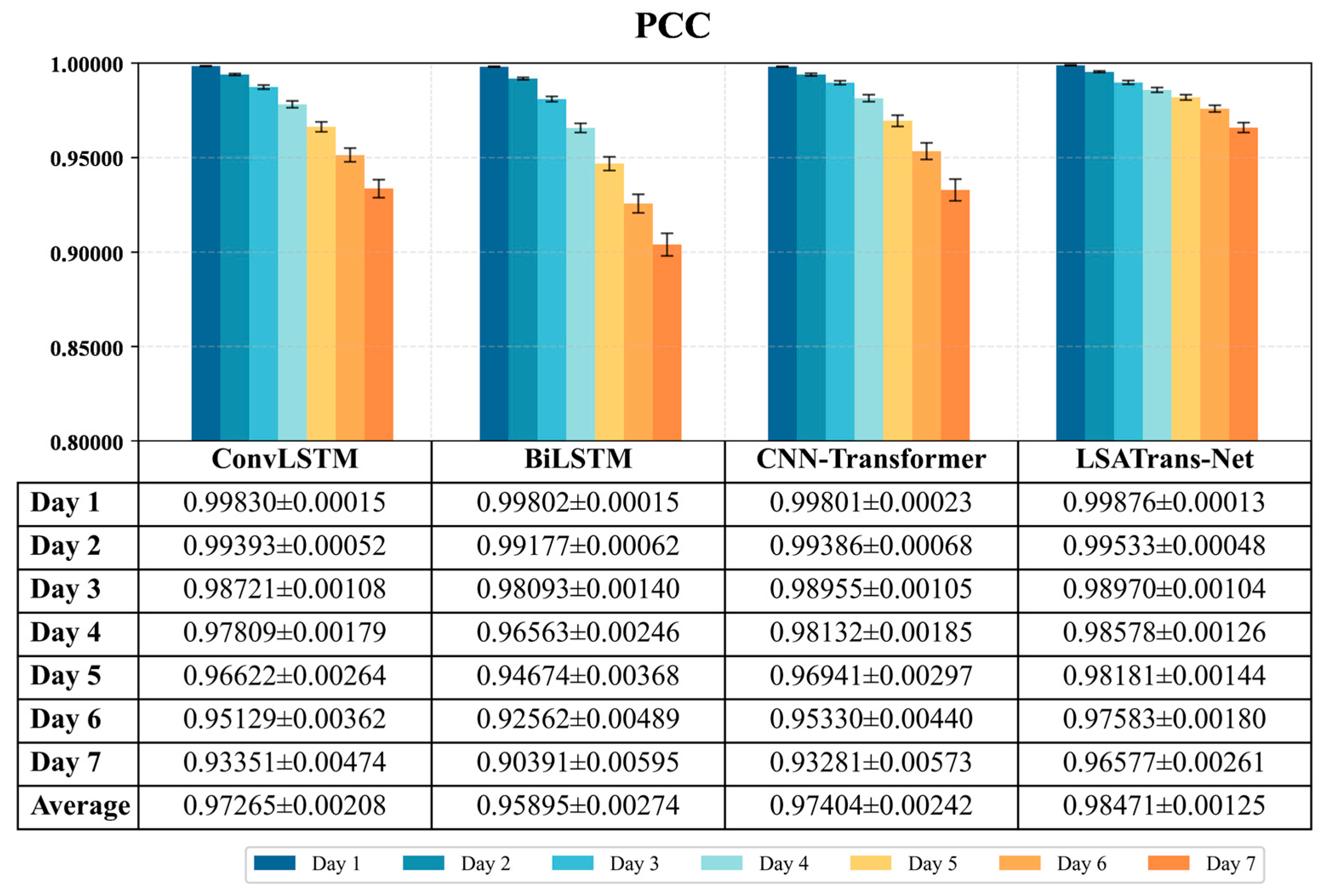
All models employ the ΔSLA data processing strategy in the prediction task to eliminate the impact of preprocessing differences on the results. Figure 5 presents the PCC comparison results over a seven-day forecast period, indicating that all four models exhibit strong spatial correlations in short-term predictions. The PCC values for the first-day predictions all exceed 0.99, while those for the third day remain above 0.98. These results demonstrate that the ΔSLA strategy effectively captures the temporal dynamics of SLA variations. As the forecast horizon increases, the performance differences among the models become more pronounced.
LSATrans-Net consistently outperforms the other models across all forecast periods, maintaining a high correlation of 0.9658 on the 7th day. As a classical spatiotemporal modeling, ConvLSTM remains highly competitive in short-term predictions (1–3 days), with PCC values exceeding 0.9870. As the forecast horizon extends, its PCC declines to 0.9335 on day 7, lower than that achieved by LSATrans-Net. BiLSTM shows relatively inferior performance among all models, with a PCC of only 0.9039 on the 7th day. This indicates that, although the bidirectional architecture can theoretically capture sequence features from both forward and backward directions, it essentially remains a one-dimensional temporal sequence modeling approach. In prediction tasks of two-dimensional spatial fields such as SLA, BiLSTM is limited in its ability to model interactions among spatial grid points, leading to a distinct performance gap relative to models with integrated spatiotemporal modeling capabilities. The comparison with the CNN-Transformer model is particularly important. During the first three days of prediction, CNN-Transformer and LSATrans-Net exhibit almost identical evaluation metrics. However, on the 7th day, CNN-Transformer achieves a PCC of 0.9328, whereas LSATrans-Net reaches 0.9658, yielding a relative improvement of 3.54%. Since the only difference between the two models is in the attention mechanism, CNN-Transformer uses self-attention and LSATrans-Net employs Local Spatial Attention, this performance gap provides direct evidence of the effectiveness of the Local Spatial Attention. The Self-Attention mechanism establishes global dependencies among all spatial positions; however, for regional ocean prediction tasks, the correlations between distant grid points may be relatively weak. By restricting the attention computation to local spatial neighborhoods, Local Spatial Attention better reflects the physical characteristics of the ocean, where interactions are strong among neighboring regions but weak over long distances, thus achieving improved predictive performance.
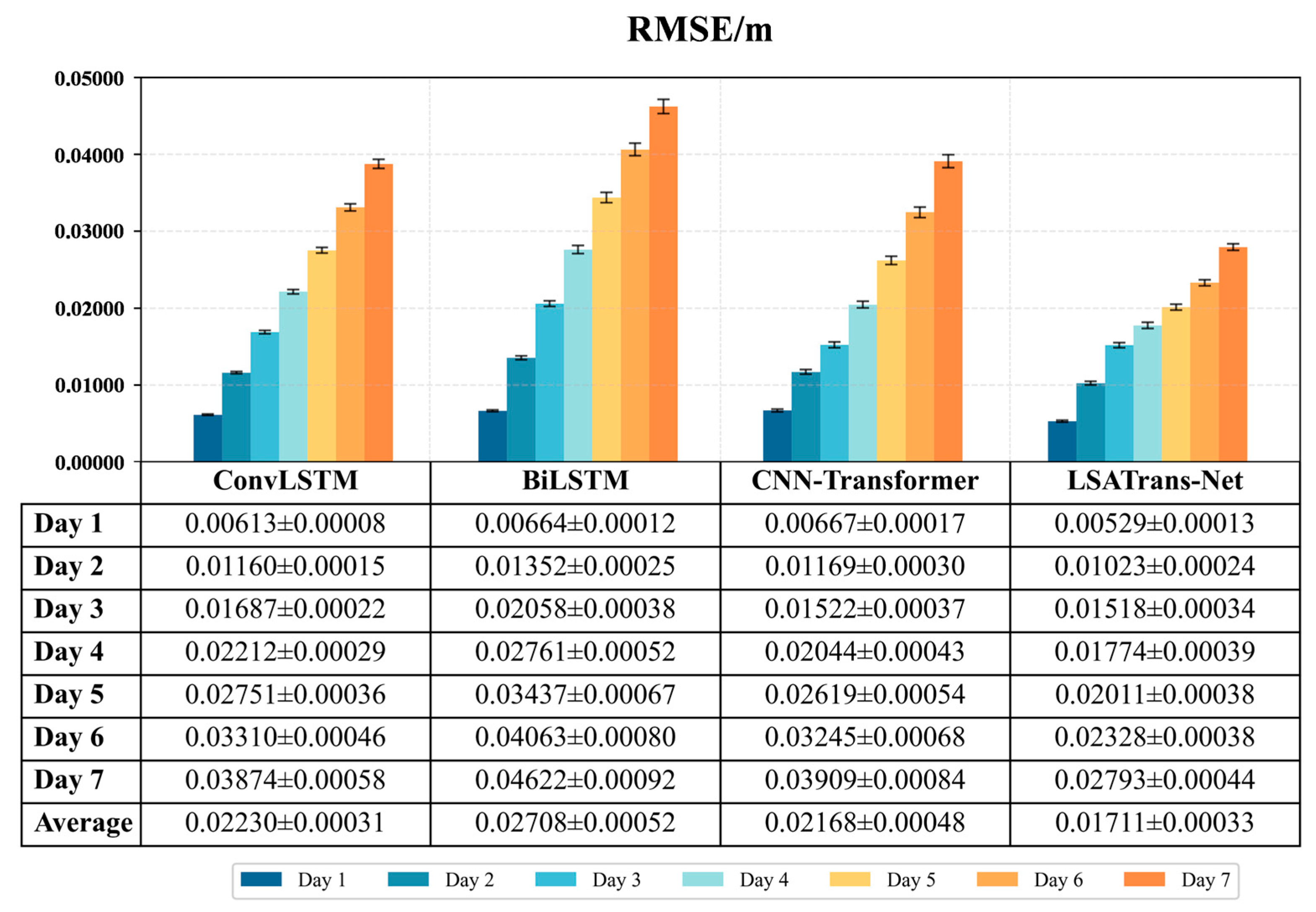
As shown in Figure 6 and Table 2, the RMSE and MAE of different models are presented over a seven-day forecast period. LSATrans-Net achieves the lowest errors across all forecast periods, with an RMSE of 0.0279 m and an MAE of 0.0211 m on the 7th day. Compared with ConvLSTM (RMSE = 0.0387 m, MAE = 0.0286 m), the errors are reduced by 27.9% and 26.2%, respectively. Relative to BiLSTM (RMSE = 0.0462 m, MAE = 0.0350 m), the reductions reach 39.6% and 39.7%, and compared with CNN-Transformer (RMSE = 0.0391 m, MAE = 0.0298 m), the reductions are 28.6% and 29.2%. These results further demonstrate that Local Spatial Attention is the key factor driving the improvement in prediction performance. Notably, LSATrans-Net exhibits the slowest rate of error accumulation. From the 1-day to the 7-day forecast, the RMSE of LSATrans-Net increases by approximately 5.3 times, compared with 6.1 times for ConvLSTM, 7.0 times for BiLSTM, and 5.8 times for CNN-Transformer. This error accumulation behavior suggests that LSATrans-Net not only enhances single-step prediction accuracy but also effectively mitigates the propagation of errors over time.
Overall, the consistency among all the evaluation metrics confirms that LSATrans-Net achieves comprehensive superiority in SLA prediction tasks across the seven days forecast horizon.
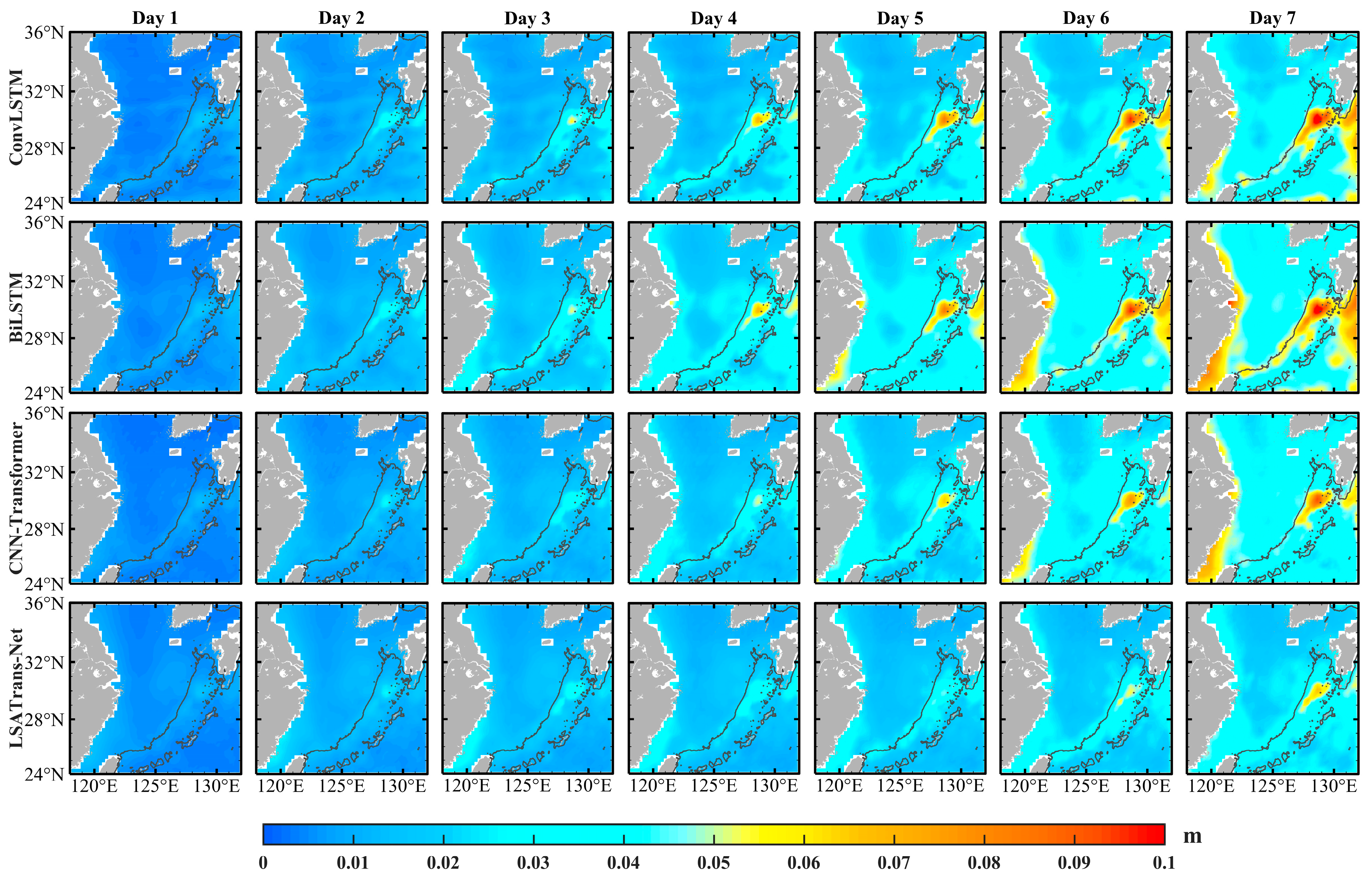
RMSE maps from different models across various lead times are shown in Figure 7, illustrating the spatial distribution of prediction errors in the study region. The first to fourth rows display RMSE maps for the ConvLSTM, BiLSTM, CNN-Transformer, and LSATrans-Net models, with lead times of 1 to 7 days, respectively. All results are based on the 2020 test dataset. For the 1-day to 3-day lead time, all four models maintain lower RMSE values, with a relatively uniform spatial distribution and no significant clusters of high errors. However, as the prediction lead time increases, performance differences between models gradually become more pronounced, particularly in the northeastern ECS-Kuroshio. The intensified ECS-Kuroshio and disappearing Ryukyu Current [42] potentially enhanced the anomalous changes in sea level in our study area, leading to higher demands on the models’ predictive capabilities.
Among all models, the BiLSTM demonstrated the weakest performance. It not only exhibited the highest numerical errors with the fastest spatial extent in the coastal region, but also showed a rapid diffusion trend in the ECS-Kuroshio region. This implied the limitations of BiLSTM in capturing complex spatial dependencies, particularly in eddy-rich regions. The CNN-Transformer model initially performed similarly to LSATrans-Net in the early 3-day forecast. However, as the forecast lead time increased, its errors accumulated more rapidly, with both the extent and intensity of high-error regions rising significantly. This indicates that, despite integrating convolutional and Transformer architectures, the Self-Attention mechanism in CNN-Transformer primarily focuses on global dependencies. Consequently, it fails to adequately model critical local spatial structures, which limits its ability to effectively capture complex spatiotemporal relationships.
In contrast, LSATrans-Net consistently exhibited the lowest and most spatially uniform RMSE across the entire 7-Day forecast period. Even in the rich-dynamic ECS-Kuroshio and coastal regions, it effectively suppressed the propagation of high errors, maintaining the RMSE below 0.07 m. These findings demonstrate the effectiveness of the LSATrans-Net model in capturing the complex temporal and spatial variations in SLA datasets, highlighting its robust performance for short-term SLA prediction tasks even in active mesoscale eddy and strong Kuroshio regions.
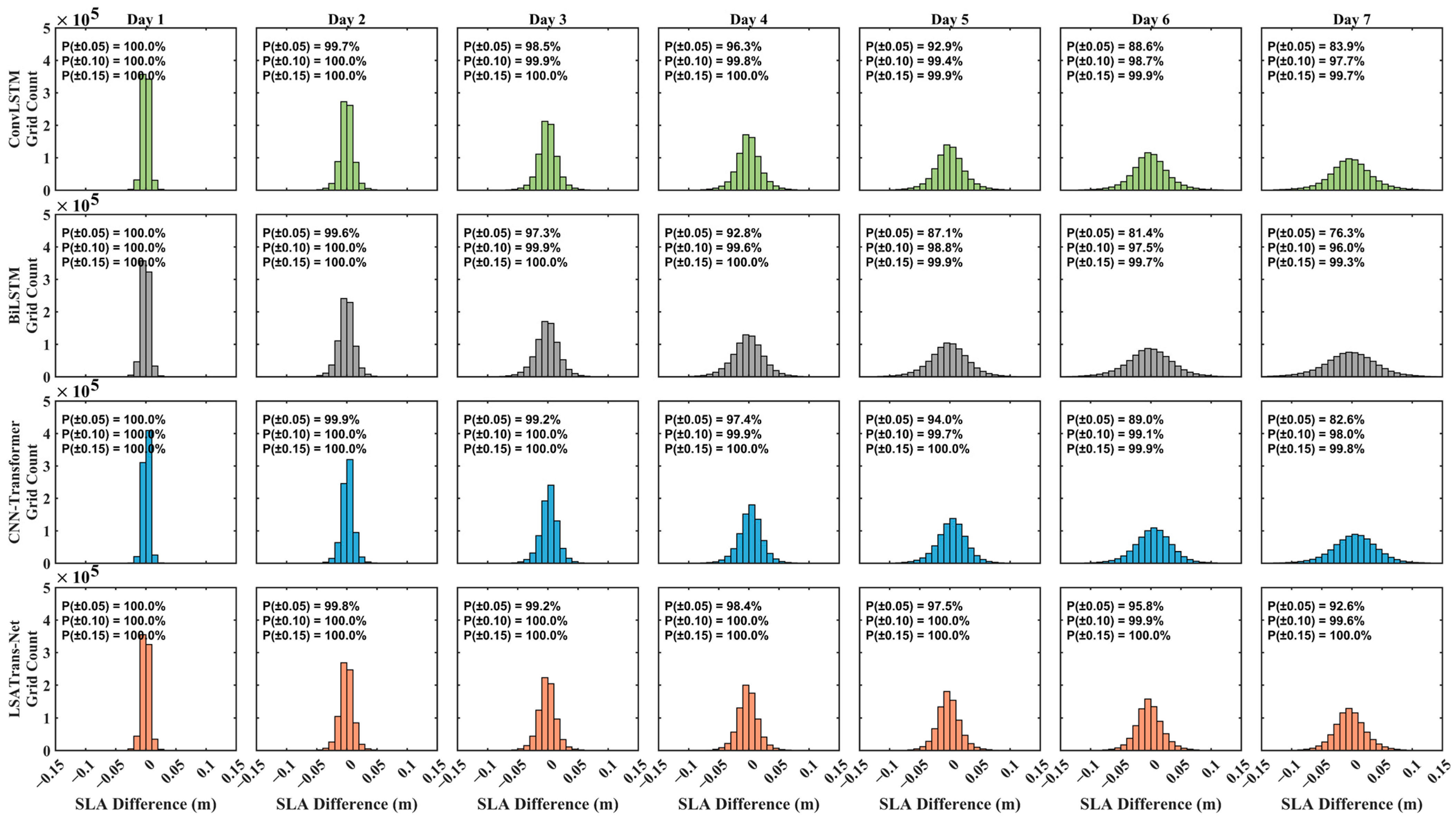
The probabilistic distribution of prediction errors offers additional statistical insights into a model’s forecasting stability. Figure 8 presents error distribution histograms for the four models at different forecast lead times. Again, the BiLSTM model exhibits the broadest error distribution, indicating the highest variability in its predictions. The ConvLSTM and CNN-Transformer models show intermediate performance, with relatively concentrated error distributions that tend to spread as lead time increases. In contrast, LSATrans-Net maintains the most concentrated error distribution across all forecast horizons, with errors tightly clustered around zero and histograms that are sharply peaked, indicating a significantly lower level of dispersion than the other models. The statistical results in Figure 8 further quantify the above findings. For the 7-day forecast, 92.6% of LSATrans-Net’s grid point errors fall within ±0.05 m, which is notably higher than those of the CNN-Transformer (82.6%), ConvLSTM (83.9%), and BiLSTM (76.3%).
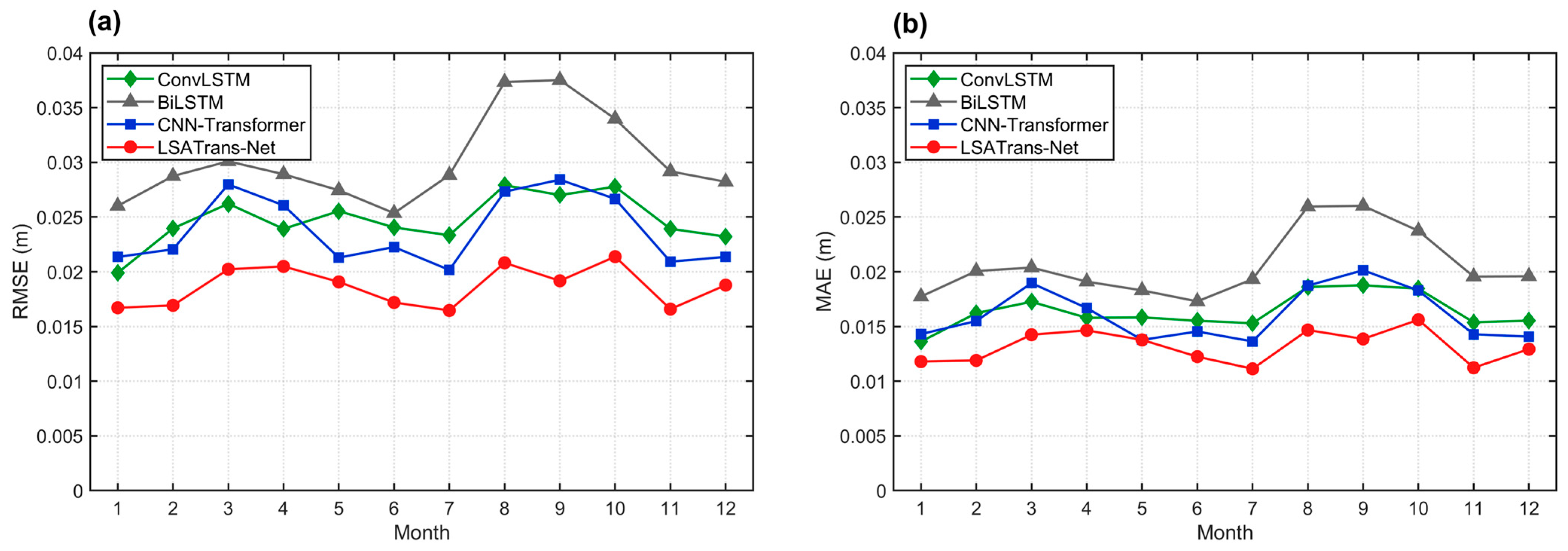
Given the pronounced seasonal variability in sea surface height, a reliable forecasting model must maintain consistent accuracy throughout the year. We further examine the monthly forecast ability of the four models over 2020 in order to check their robustness and stability under a seasonal timescale. Figure 9 illustrates the monthly averaged RMSE and MAE from four models in 2020. All models exhibit seasonal fluctuations, but the degree of fluctuation varies. Among them, the BiLSTM model demonstrates the most pronounced fluctuations, indicating poorer stability, while ConvLSTM and CNN-Transformer exhibit intermediate fluctuations, but with overall higher error levels. In comparison, LSATrans-Net consistently achieves the lowest RMSE and MAE across all months. Its error curves are characterized by the lowest overall magnitude and the smallest fluctuations, demonstrating the greatest insensitivity to SLA seasonal variability along with the highest robustness.
Additionally, Figure 9 highlights a noteworthy increase in prediction errors for all models from August to October. This is probably associated with the frequent occurrence of extreme weather events such as typhoons around the study region during this season, demonstrating that such meteorological extremes considerably degrade forecast accuracy across all models.
Through a multi-faceted assessment, the LSATrans-Net model is demonstrated as a more reliable choice for SLA forecasting in ECS. Leveraging the Local Spatial Attention mechanisms, it adheres more closely to the principle of physical proximity, effectively captures key local spatial variations, and generates SLA predictions with more accurate spatial structures and superior error control.

4.2. Performance Under Representative Cases

To thoroughly assess the forecasting capability of LSATrans-Net under varying weather conditions, this section examines its forecasting performance under two representative scenarios. First, a relatively stable sea surface evolution under normal weather conditions; second, a scenario involving intense sea level changes during extreme weather, such as typhoons. By evaluating predictive performance across these two scenarios, we examine both the model’s baseline forecasting capability under normal weather conditions and its robustness and adaptability during extreme weather events.

4.2.1. Normal Weather Conditions

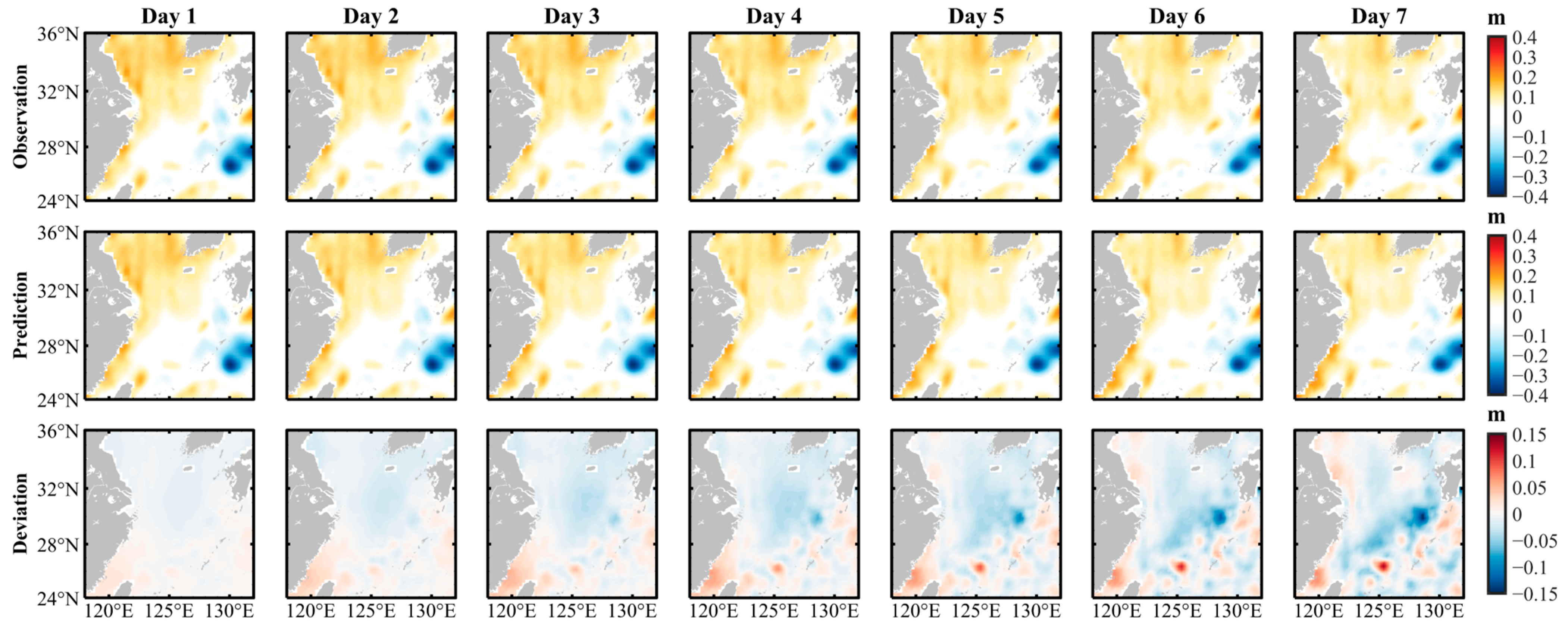
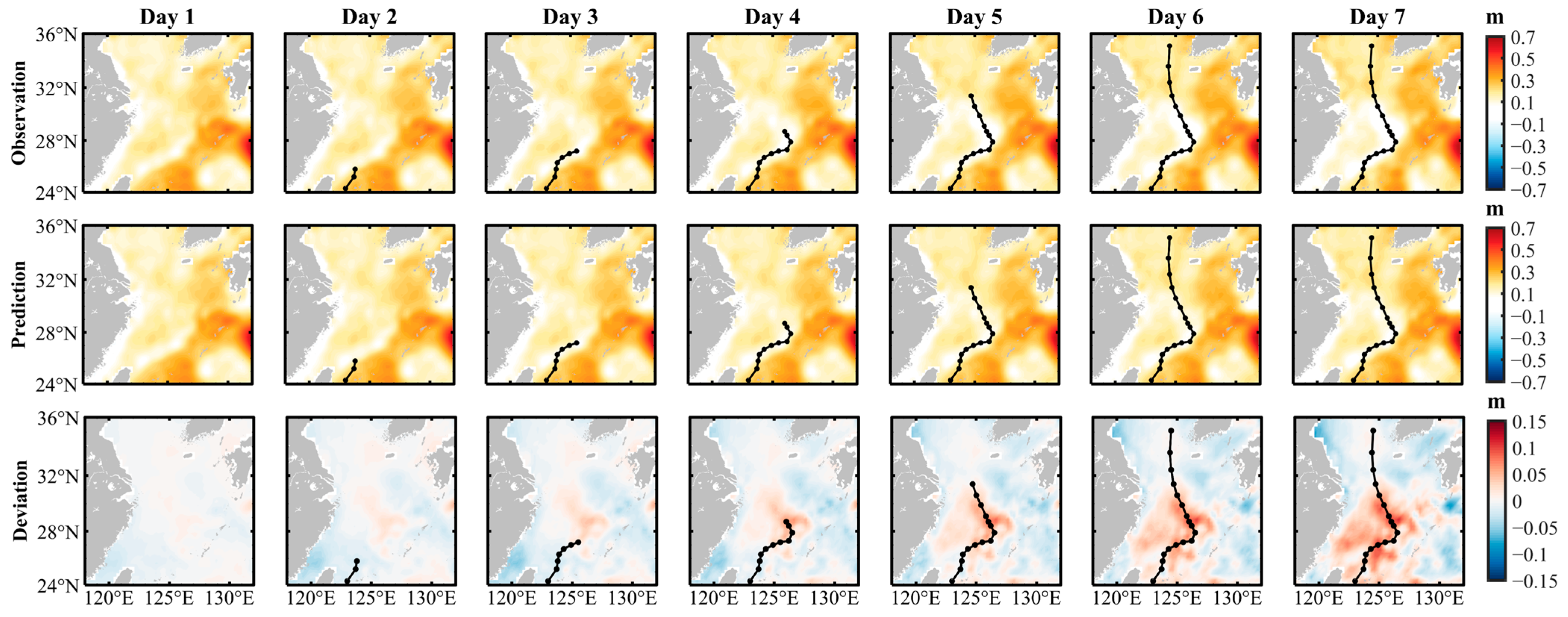
First, we evaluate the baseline forecasting capability of the LSATrans-Net model under normal weather conditions. Figure 10 presents the observed and predicted SLA from February 1st to 7th, 2020. The first row shows the satellite-observed SLA fields, the second row displays the model predictions, and the third row presents the forecast deviations. Here, we employ the method of subtracting observed values from predicted values. Therefore, a positive deviation indicates that the model predicted values are relatively high, while a negative deviation means that the model predicted values are relatively low.
By comparing daily SLA deviation in the third row of Figure 10, it is evident that the LSATrans-Net model effectively captures the variation in daily SLA distribution within the study area. The prediction errors consistently remained within ±0.05 m over the majority of the study area, with no significant degradation in deviation patterns. The location and intensity of multiple main mesoscale eddies around ECS-Kuroshio are also well reproduced. Notably, slightly larger deviations, approximately ±0.1 m, sporadically appeared in the ECS-Kuroshio front region, where the largest SLA gradient was observed, which is mainly due to the complex dynamic processes in this area. In summary, this case demonstrates that LSATrans-Net possesses stable and accurate baseline forecasting capabilities under normal weather conditions.

4.2.2. Extreme Weather Conditions

Super Typhoon Bavi in 2020 was selected as a representative case to assess the model’s performance during extreme weather events. As indicated by the black dot line in Figure 11, Bavi began as a tropical depression on 21 August, and gradually strengthened between Taiwan and Okinawa over the western north Pacific and moved northward and strengthened into a tropical storm on 22 August. It experienced a brief rapid intensification followed by a slow intensification from 23 August, and it moved east-northeastward. It suddenly turned northwestward and upgraded to a typhoon by 24 August. Bavi further intensified to a severe typhoon on 25 August, turned to the north, and reached its peak intensity on 26 August. Afterwards, Bavi continued moving northward and weakened rapidly on 27 August [43], finally landfalling over North Korea.
Daily SLA from 21 to 27 August during the Super Typhoon Bavi period was presented in Figure 11, in which the observed SLA fields were shown in the second row. From this, an obvious positive SLA covered the ECS, implying that a widespread sea level rise ahead of Typhoon Bavi occurred in the study area. Meanwhile, a significant negative SLA emerged along the path of Typhoon Bavi as it crossed the ECS. These variations in SLA were well captured by the LSATrans-Net model, as shown in the third row of Figure 11.
From 21 August to 23 August, the deviation in the first row of Figure 11 generally remained within ±0.05 m, suggesting that the LSATrans-Net model captured the spatiotemporal evolution of sea level variation at the initial growth stage of the typhoon event well. However, as the forecast lead time extended, the prediction accuracy exhibited degradation corresponding to typhoon intensification. As the typhoon advanced and rapidly intensified from 24 to 26 August, the observed negative SLA progressively awakened, while the model’s predictions did not fully capture this pattern. Deviation increased with the prediction lead time, with +0.1 m biases concentrated along the track of Bavi. This underestimation potentially stems from the fundamental limitation of our single-variable input approach. During Bavi’s rapid intensification phase, SLA changes became increasingly dominated by rapidly intensifying atmospheric forcing rather than ocean internal dynamics [44]. Without explicit information about evolving wind stress and atmospheric pressure fields, our model cannot accurately predict the changes in SLA under strong typhoons, resulting in a positive bias of approximately +0.12 m along the trajectory region of Bavi.
These findings reveal that under extreme weather conditions, the prediction lead time is recommended to be limited to 3 days for the LSATrans-Net model and multiple variables should be incorporated to improve the capability of SLA prediction during typhoon intensification.

4.3. Differential Strategy Experiment

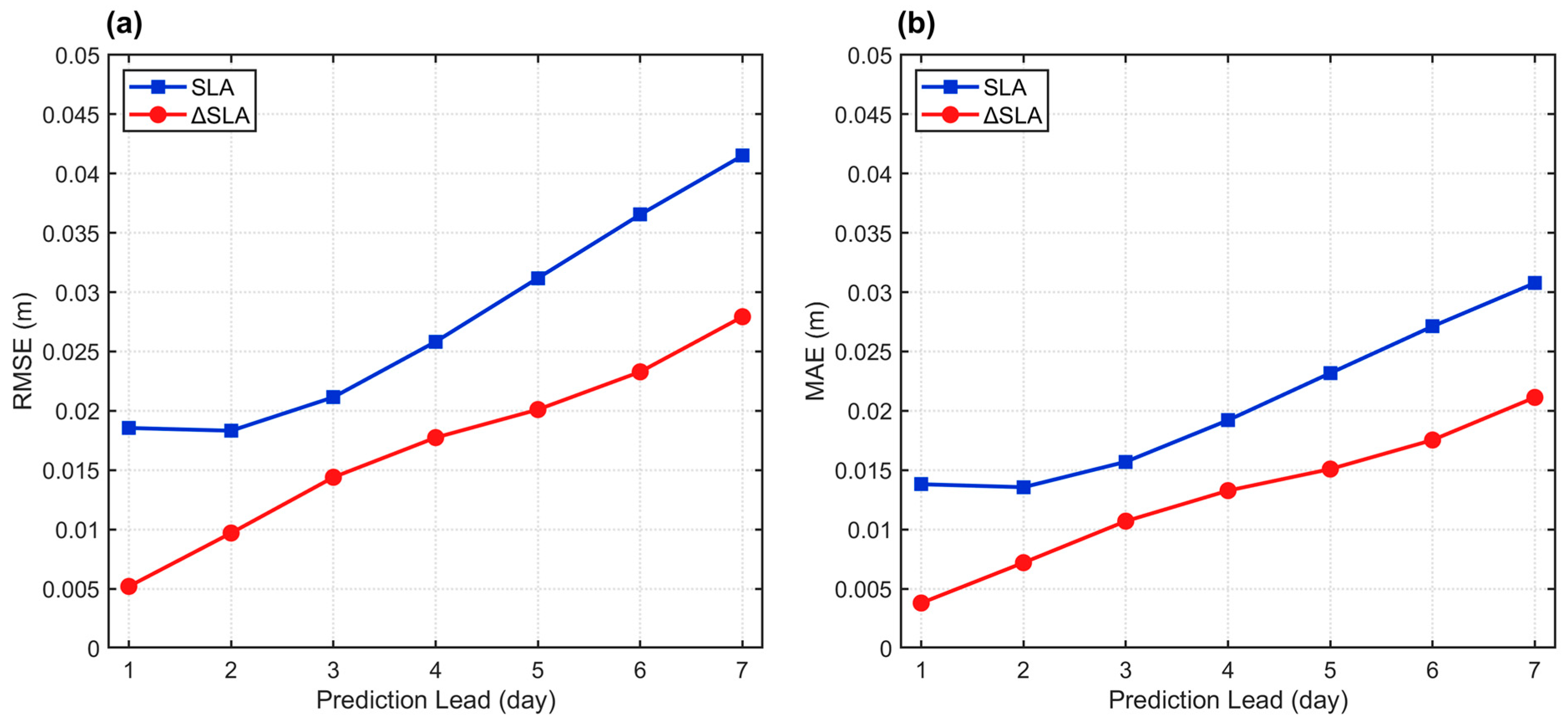
To quantitatively assess the advantages of using sea level anomaly increments (ΔSLA) for forecasting, we designed a set of comparative experiments based on the established LSATrans-Net model. These experiments conducted rigorous side-by-side comparisons between two forecasting strategies, both utilizing identical network architectures and hyperparameter settings, with the only difference being the data processing. Specifically, the baseline SLA-Forecast strategy directly inputs historical SLA value sequences and undergoes end-to-end training, with future direct SLA values as the target for prediction. In contrast, the ΔSLA-Forecast strategy applies first-order differencing to the raw SLA time series to generate an increment (ΔSLA) sequence. This sequence is then used as input to forecast future increments, and the model’s output is reconstructed into the future SLA value through cumulative summation.
By strictly controlling the sole variable, this experiment ensures that the performance differences between the two strategies reflect the efficacy disparity between SLA and ΔSLA. Figure 12 gives the daily RMSE and MAE for both the SLA-Forecast and ΔSLA-Forecast strategies. The results indicate that ΔSLA-Forecast outperforms SLA-Forecast across all forecast lead times, with its error curve consistently lying below that of SLA-Forecast. Moreover, the error curve profiles highlight distinct differences between the two strategies. SLA-Forecast shows a gradual increase in RMSE and MAE over the first two days, indicating that LSATrans-Net can effectively capture and utilize the inertia of the ocean state. However, as the forecast lead time extends, the direct prediction of SLA values leads to accelerated error accumulation. In contrast, ΔSLA-Forecast exhibits a lower rate of error growth and smoother curves from the outset, demonstrating superior stability in 7-day forecasting.
This comparison clearly demonstrates the advantages of using a differential approach to generate ΔSLA as model training data. By directly converting the prediction target into an incremental sequence, this method is more concise and straightforward, significantly reducing data processing complexity. As a result, LSATrans-Net can focus on modeling ocean dynamic processes, effectively enhancing the stability and robustness of 7-day predictions without substantially increasing computational cost.
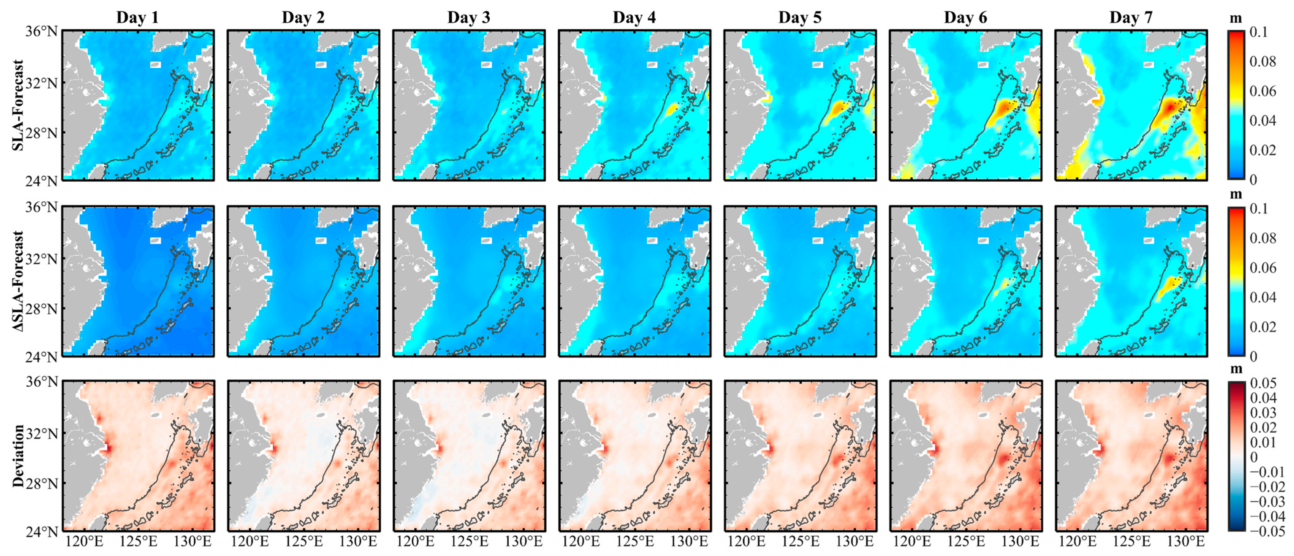
To further validate the superiority of the ΔSLA-Forecast prediction strategy, Figure 13 illustrates the spatial distribution of daily RMSE from both methods over a 7-day forecast period. As shown in the first row of Figure 13, the SLA-Forecast predictions exhibit a pronounced error accumulation during the latter stages of the forecast task. Though RMSE remains low during the early 1 to 2 forecast days, a performance inflection point becomes apparent from day 3 onwards. In mesoscale eddy-rich regions such as the ECS-Kuroshio, coastal regions such as SCC, CDW, ZMCC and the Taiwan Strait, high-error clusters gradually form, with RMSE steadily increasing over the forecast period. RMSE rises from approximately 0.04 m to exceed 0.08 m by day 7. These results suggest that the inherent nonlinear and non-stationary characteristics of the SLA sequence render predictions based directly on SLA values inadequate for accurately capturing its complex dynamic evolution, leading to persistent error accumulation.
In contrast, the ΔSLA-Forecast consistently maintained lower prediction errors with a relatively uniform spatial distribution throughout the entire forecast period, demonstrating superior generalization capability and robustness, as shown in the second row of Figure 13. Particularly in dynamically active regions such as the ECS-Kuroshio, northeastern Ryukyu and Taiwan Strait, the ΔSLA-Forecast errors remained significantly lower than those of the SLA-Forecast. This advantage is further quantified in the third row of Figure 13, which displays the deviation (SLA-Forecast minus ΔSLA-Forecast). The predominantly positive values (red regions) across most of the domain confirm that the ΔSLA-Forecast strategy consistently outperforms the SLA-Forecast strategy. By day 7, the RMSE difference reaches 0.03–0.05 m.
Based on the analysis of quantitative metrics and spatial error distributions, we conclude that transforming the prediction task from SLA to ΔSLA effectively reduces the model’s learning complexity, enabling the LSATrans-Net model to characterize internal oceanic dynamics better. This strategy achieves superior prediction accuracy and enhanced physical fidelity without incurring substantial computational costs, striking an excellent balance between performance and efficiency, making it a valuable approach for high-precision SLA forecasting.

5. Conclusions

This paper presents the LSATrans-Net model for short-term SLA prediction in the regional East China Sea, integrating a first-order difference preprocessing strategy with the Local Spatial Attention mechanisms. By optimizing both data processing and model architecture in a synergistic manner, the model achieves a favorable balance between predictive accuracy and physical plausibility.
In terms of model architecture, a Local Spatial Attention mechanism is incorporated within the Transformer encoder. Attention calculations for each grid point are restricted to its neighboring region, which enhances the model’s ability to capture marine mesoscale dynamic processes. This design is consistent with the “neighborhood effect” observed in actual ocean dynamics.
For data processing, the first-order difference preprocessing strategy turns the non-stationary SLA sequence into an incremental sequence of adjacent time steps, emphasizing short-term dynamic variations. This approach effectively mitigates interference from long-term trends and seasonal signals, allowing the model to focus more acutely on rapid internal oceanic processes.
Through multi-dimensional quantitative metrics and systematic case studies, LSATrans-Net demonstrates superior performance compared to ConvLSTM, BiLSTM and CNN-Transformer, across all evaluation indicators (RMSE, MAE, PCC) for the 7-day forecasting task. The model shows the lowest cumulative error rate across forecast lead times and exhibits the most uniform spatial distribution. Its advantages are particularly pronounced in dynamically complex regions such as the Kuroshio and eddy-rich regions. Additionally, monthly performance evaluations and case studies of typical weather conditions further validate the model’s stability and physical consistency under varying seasonal conditions and extreme weather events. Compared to forecasts based directly on SLA strategy, the ΔSLA differential strategy significantly reduces error accumulation during multi-step extrapolation, thereby improving forecast accuracy and stability.
Although this study has achieved the intended outcomes, several avenues for further exploration remain. The current model uses only SLA as input and does not incorporate other multimodal environmental variables, such as wind, sea level pressure or sea surface temperature, which limits its ability to respond to external forcing under complex dynamic conditions. The model’s generalizability and physical consistency can be enhanced by integrating additional variables and physics-based constraints. Additionally, the fixed neighborhood radius and shape in the Local Spatial Attention mechanism potentially restrict the model’s adaptability to oceanic processes across different scales. Future iterations should allow dynamic adjustments of neighborhood ranges based on the characteristics of the dynamic processes, enabling more flexible spatiotemporally variable attention modeling.

Author Contributions

Conceptualization, Y.W., L.J. and Q.J.; methodology, Y.W., L.J. and H.C.; software, G.H. and J.L.; validation, Y.W., J.L. and J.W.; formal analysis, Y.W., H.C. and Q.J.; investigation, Y.W. and J.W.; data curation, L.J., Y.W. and G.H.; writing—original draft preparation, Y.W. and Q.J.; writing—review and editing, Y.W., H.C., L.J., Q.J., J.L., J.W. and G.H.; visualization, J.L. and G.H.; supervision, H.C. and Q.J.; project administration, H.C., Q.J. and J.W. All authors have read and agreed to the published version of the manuscript.

Funding

This research is supported by the Zhejiang Provincial Financial General Public Budget Project “Impact Analysis of Sea Level Rise” (No. 330000210130313013006) and the National Key Research and Development Program of China (No. 2023YFD2401904).

Data Availability Statement

Publicly available datasets were analyzed in this study. The SLA data used in this study was obtained from Copernicus Marine Service (https://doi.org/10.48670/moi-00148). All figures were generated using MATLAB 2024 and Python 3.8.

Acknowledgments

The authors would like to thank the Copernicus Marine Service for providing the SEALEVEL_GLO_PHY_L4_MY_008_047 sea level data product free of charge.

Conflicts of Interest

The authors declare no conflicts of interest.

Appendix A

To validate the choice of spatial radius r = 1, a sensitivity analysis was conducted by varying r across values of 1, 3, and 5, corresponding to effective spatial ranges of approximately 100 km, 300 km, and 500 km, respectively. Table A1 and Table A2 present the PCC and RMSE results over the 7-day forecast period.
The results demonstrate that r = 1 achieves the best performance, with an average PCC of 0.985 and RMSE of 0.017 m. This scale matching ensures that the Local Spatial Attention mechanism focuses on the most dynamically relevant spatial correlations while filtering out noise from weakly correlated distant regions. Notably, as the attention radius increases from r = 1 to r = 3 and r = 5, the model incorporates progressively more spatial information from larger neighborhoods (3 × 3, 7 × 7, and 11 × 11 grid cells, respectively). However, rather than improving predictive performance, this additional information leads to monotonic performance degradation, with RMSE increasing and PCC declining.
These results confirm that the ±100 km range of r = 1 optimally matches the dominant spatial scales of physical dynamic progress in the ECS, both the Kuroshio and the mesoscale eddies. Larger radius incorporates information from distant regions with weaker physical correlations, diluting attention weights and degrading prediction accuracy.
Table A1. Daily and average PCC comparison results of different spatial radii over a 7-Day forecast period.
Spatial RadiusEffective RangeDay 1Day 2Day 3Day 4Day 5Day 6Day 7Average
1100 km0.998760.995330.989700.985780.981810.975830.965770.98471
3300 km0.998680.995210.989540.982140.975240.965970.952750.97993
5500 km0.998600.995090.989380.980020.970640.958800.943780.97662
Table A2. Daily and average RMSE comparison results of different spatial radii over a 7-Day forecast period.
Spatial RadiusEffective RangeDay 1Day 2Day 3Day 4Day 5Day 6Day 7Average
1100 km0.005290.010230.015180.017740.020110.023280.027930.01711
3300 km0.005370.010350.015330.020220.023840.027980.033040.01945
5500 km0.005450.010470.015480.020930.025350.030060.035190.02042

References

  1. Nicholls, R.J.; Cazenave, A. Sea-Level Rise and Its Impact on Coastal Zones. Science 2010, 328, 1517–1520. [Google Scholar] [CrossRef] [PubMed]
  2. Horton, B.P.; Kopp, R.E.; Garner, A.J.; Hay, C.C.; Khan, N.S.; Roy, K.; Shaw, T.A. Mapping Sea-Level Change in Time, Space, and Probability. Annu. Rev. Environ. Resour. 2018, 43, 481–521. [Google Scholar] [CrossRef]
  3. Hu, Z.-Z.; Kumar, A.; Huang, B.; Zhu, J.; Zhang, R.-H.; Jin, F.-F. Asymmetric evolution of El Niño and La Niña: The recharge/discharge processes and role of the off-equatorial sea surface height anomaly. Clim. Dyn. 2017, 49, 2737–2748. [Google Scholar] [CrossRef]
  4. Widlansky, M.J.; Long, X.; Schloesser, F. Increase in sea level variability with ocean warming associated with the nonlinear thermal expansion of seawater. Commun. Earth Environ. 2020, 1, 9. [Google Scholar] [CrossRef]
  5. Liu, Z.; Gan, J.; Hu, J.; Wu, H.; Cai, Z.; Deng, Y. Progress on circulation dynamics in the East China Sea and southern Yellow Sea: Origination, pathways, and destinations of shelf currents. Prog. Oceanogr. 2021, 193, 102553. [Google Scholar] [CrossRef]
  6. Li, Y.; Gao, J.; Yin, J.; Wu, S. Assessing the potential of compound extreme storm surge and precipitation along China’s coastline. Weather Clim. Extrem. 2024, 45, 100702. [Google Scholar] [CrossRef]
  7. Qu, Y.; Jevrejeva, S.; Jackson, L.P.; Moore, J.C. Coastal Sea level rise around the China Seas. Glob. Planet. Change 2019, 172, 454–463. [Google Scholar] [CrossRef]
  8. Yin, J.; Yin, Z.; Wang, J.; Xu, S. National assessment of coastal vulnerability to sea-level rise for the Chinese coast. J. Coast. Conserv. 2012, 16, 123–133. [Google Scholar] [CrossRef]
  9. Cheng, Y.; Plag, H.-P.; Hamlington, B.D.; Xu, Q.; He, Y. Regional sea level variability in the Bohai Sea, Yellow Sea, and East China Sea. Cont. Shelf Res. 2015, 111, 95–107. [Google Scholar] [CrossRef]
  10. Zhou, D.; Liu, Y.; Feng, Y.; Zhang, H.; Fu, Y.; Liu, Y.; Tang, Q. Absolute Sea Level Changes Along the Coast of China from Tide Gauges, GNSS, and Satellite Altimetry. J. Geophys. Res. Oceans 2022, 127, e2022JC018994. [Google Scholar] [CrossRef]
  11. Storkey, D.; Blockley, E.W.; Furner, R.; Guiavarc’h, C.; Lea, D.; Martin, M.J.; Barciela, R.M.; Hines, A.; Hyder, P.; Siddorn, J.R. Forecasting the ocean state using NEMO:The new FOAM system. J. Oper. Oceanogr. 2010, 3, 3–15. [Google Scholar] [CrossRef]
  12. Miles, E.R.; Spillman, C.M.; Church, J.A.; McIntosh, P.C. Seasonal prediction of global sea level anomalies using an ocean–atmosphere dynamical model. Clim. Dyn. 2014, 43, 2131–2145. [Google Scholar] [CrossRef]
  13. Frederikse, T.; Lee, T.; Wang, O.; Kirtman, B.; Becker, E.; Hamlington, B.; Limonadi, D.; Waliser, D. A Hybrid Dynamical Approach for Seasonal Prediction of Sea-Level Anomalies: A Pilot Study for Charleston, South Carolina. J. Geophys. Res. Oceans 2022, 127, e2021JC018137. [Google Scholar] [CrossRef]
  14. Srivastava, P.K.; Islam, T.; Singh, S.K.; Petropoulos, G.P.; Gupta, M.; Dai, Q. Forecasting Arabian Sea level rise using exponential smoothing state space models and ARIMA from TOPEX and Jason satellite radar altimeter data. Meteorol. Appl. 2016, 23, 633–639. [Google Scholar] [CrossRef]
  15. Xue, Y.; Leetmaa, A. Forecasts of tropical Pacific SST and sea level using a Markov model. Geophys. Res. Lett. 2000, 27, 2701–2704. [Google Scholar] [CrossRef]
  16. Chowdhury, M.R.; Chu, P.S.; Schroeder, T.; Colasacco, N. Seasonal sea-level forecasts by canonical correlation analysis—An operational scheme for the US-affiliated Pacific Islands. Int. J. Climatol. J. R. Meteorol. Soc. 2007, 27, 1389–1402. [Google Scholar] [CrossRef]
  17. Braakmann-Folgmann, A.; Roscher, R.; Wenzel, S.; Uebbing, B.; Kusche, J. Sea level anomaly prediction using recurrent neural networks. arXiv 2017, arXiv:1710.07099. [Google Scholar] [CrossRef]
  18. Patil, K.; Deo, M.C.; Ravichandran, M. Prediction of Sea Surface Temperature by Combining Numerical and Neural Techniques. J. Atmos. Ocean. Technol. 2016, 33, 1715–1726. [Google Scholar] [CrossRef]
  19. Sun, Q.; Wan, J.; Liu, S. Estimation of Sea Level Variability in the China Sea and Its Vicinity Using the SARIMA and LSTM Models. IEEE J. Sel. Top. Appl. Earth Obs. Remote Sens. 2020, 13, 3317–3326. [Google Scholar] [CrossRef]
  20. Winona, A.Y.; Adytia, D. Short Term Forecasting of Sea Level by Using LSTM with Limited Historical Data. In Proceedings of the 2020 International Conference on Data Science and Its Applications, Bandung, Indonesia, 5–6 August 2020; pp. 1–5. [Google Scholar]
  21. Balogun, A.-L.; Adebisi, N. Sea level prediction using ARIMA, SVR and LSTM neural network: Assessing the impact of ensemble Ocean-Atmospheric processes on models’ accuracy. Geomat. Nat. Hazards Risk 2021, 12, 653–674. [Google Scholar] [CrossRef]
  22. Ma, C.; Li, S.; Wang, A.; Yang, J.; Chen, G. Altimeter Observation-Based Eddy Nowcasting Using an Improved Conv-LSTM Network. Remote Sens. 2019, 11, 783. [Google Scholar] [CrossRef]
  23. Han, L.; Ji, Q.; Jia, X.; Liu, Y.; Han, G.; Lin, X. Significant Wave Height Prediction in the South China Sea Based on the ConvLSTM Algorithm. J. Mar. Sci. Eng. 2022, 10, 1683. [Google Scholar] [CrossRef]
  24. Hao, P.; Li, S.; Song, J.; Gao, Y. Prediction of Sea Surface Temperature in the South China Sea Based on Deep Learning. Remote Sens. 2023, 15, 1656. [Google Scholar] [CrossRef]
  25. Pascanu, R.; Mikolov, T.; Bengio, Y. On the difficulty of training recurrent neural networks. In Proceedings of the International Conference on Machine Learning, Atlanta, GA, USA, 16–21 June 2013; pp. 1310–1318. [Google Scholar]
  26. Shi, X.; Chen, Z.; Wang, H.; Yeung, D.-Y.; Wong, W.-K.; Woo, W.-C. Convolutional LSTM network: A machine learning approach for precipitation nowcasting. Adv. Neural Inf. Process. Syst. 2015, 28, 802–810. [Google Scholar] [CrossRef]
  27. Vaswani, A.; Shazeer, N.; Parmar, N.; Uszkoreit, J.; Jones, L.; Gomez, A.N.; Kaiser, Ł.; Polosukhin, I. Attention is all you need. Adv. Neural Inf. Process. Syst. 2017, 30, 5998–6008. [Google Scholar] [CrossRef]
  28. Zhang, T.; Lin, P.; Liu, H.; Wang, P.; Wang, Y.; Zheng, W.; Yu, Z.; Jiang, J.; Li, Y.; He, H. A New Transformer Network for Short-Term Global Sea Surface Temperature Forecasting: Importance of Eddies. Remote Sens. 2025, 17, 1507. [Google Scholar] [CrossRef]
  29. Wu, S.; Bao, S.; Dong, W.; Wang, S.; Zhang, X.; Shao, C.; Zhu, J.; Li, X. PGTransNet: A physics-guided transformer network for 3D ocean temperature and salinity predicting in tropical Pacific. Front. Mar. Sci. 2024, 11, 1477710. [Google Scholar] [CrossRef]
  30. Wang, L.; Zhang, X.; Leung, L.R.; Chiew, F.H.; AghaKouchak, A.; Ying, K.; Zhang, Y. CAS-Canglong: A skillful 3D Transformer model for sub-seasonal to seasonal global sea surface temperature prediction. arXiv 2024, arXiv:2409.05369. [Google Scholar] [CrossRef]
  31. Miller, H.J. Tobler’s First Law and Spatial Analysis. Ann. Assoc. Am. Geogr. 2004, 94, 284–289. [Google Scholar] [CrossRef]
  32. Wiatowski, T.; Bölcskei, H. A Mathematical Theory of Deep Convolutional Neural Networks for Feature Extraction. IEEE Trans. Inf. Theory 2018, 64, 1845–1866. [Google Scholar] [CrossRef]
  33. Wang, B.; Wang, B.; Wu, W.; Xi, C.; Wang, J. Sea-water-level prediction via combined wavelet decomposition, neuro-fuzzy and neural networks using SLA and wind information. Acta Oceanol. Sin. 2020, 39, 157–167. [Google Scholar] [CrossRef]
  34. Chen, H.; Lu, T.; Huang, J.; He, X.; Sun, X. An Improved VMD–EEMD–LSTM Time Series Hybrid Prediction Model for Sea Surface Height Derived from Satellite Altimetry Data. J. Mar. Sci. Eng. 2023, 11, 2386. [Google Scholar] [CrossRef]
  35. Shao, Q.; Li, W.; Han, G.; Hou, G.; Liu, S.; Gong, Y.; Qu, P. A Deep Learning Model for Forecasting Sea Surface Height Anomalies and Temperatures in the South China Sea. J. Geophys. Res. Oceans 2021, 126, e2021JC017515. [Google Scholar] [CrossRef]
  36. Pokhrel, P.; Ioup, E.; Simeonov, J.; Hoque, M.T.; Abdelguerfi, M. A Transformer-Based Regression Scheme for Forecasting Significant Wave Heights in Oceans. IEEE J. Ocean. Eng. 2022, 47, 1010–1023. [Google Scholar] [CrossRef]
  37. Lopez, B. Regional Sea Level Rise Prediction in Monterey Bay with LSTMs and Vertical Land Motion. Master’s Thesis, San José State University, San Jose, CA, USA, 2024. [Google Scholar] [CrossRef]
  38. Liu, Z.; Gan, J. Variability of the Kuroshio in the East China Sea derived from satellite altimetry data. Deep Sea Res. Part I Oceanogr. Res. Pap. 2012, 59, 25–36. [Google Scholar] [CrossRef]
  39. Qin, D.; Wang, J.; Liu, Y.; Dong, C. Eddy analysis in the Eastern China Sea using altimetry data. Front. Earth Sci. 2015, 9, 709–721. [Google Scholar] [CrossRef]
  40. Avenas, A.; Mouche, A.; Tandeo, P.; Piolle, J.-F.; Chavas, D.; Fablet, R.; Knaff, J.; Chapron, B. Reexamining the Estimation of Tropical Cyclone Radius of Maximum Wind from Outer Size with an Extensive Synthetic Aperture Radar Dataset. Mon. Weather Rev. 2023, 151, 3169–3189. [Google Scholar] [CrossRef]
  41. Zrira, N.; Kamal-Idrissi, A.; Farssi, R.; Khan, H.A. Time series prediction of sea surface temperature based on BiLSTM model with attention mechanism. J. Sea Res. 2024, 198, 102472. [Google Scholar] [CrossRef]
  42. Yang, H.; Cai, J.; Wu, L.; Guo, H.; Chen, Z.; Jing, Z.; Gan, B. The Intensifying East China Sea Kuroshio and Disappearing Ryukyu Current in a Warming Climate. Geophys. Res. Lett. 2024, 51, e2023GL106944. [Google Scholar] [CrossRef]
  43. Wang, H.; Yu, Y.; Xu, H.; Zhao, D.; Liang, J. A numerical study on the effects of a midlatitude upper-level trough on the track and intensity of Typhoon Bavi (2020). Front. Earth Sci. 2023, 10, 1056882. [Google Scholar] [CrossRef]
  44. Cui, H.; Tang, D.; Liu, H.; Sui, Y.; Gu, X. Composite Analysis-Based Machine Learning for Prediction of Tropical Cyclone-Induced Sea Surface Height Anomaly. IEEE J. Sel. Top. Appl. Earth Obs. Remote Sens. 2023, 16, 2644–2653. [Google Scholar] [CrossRef]
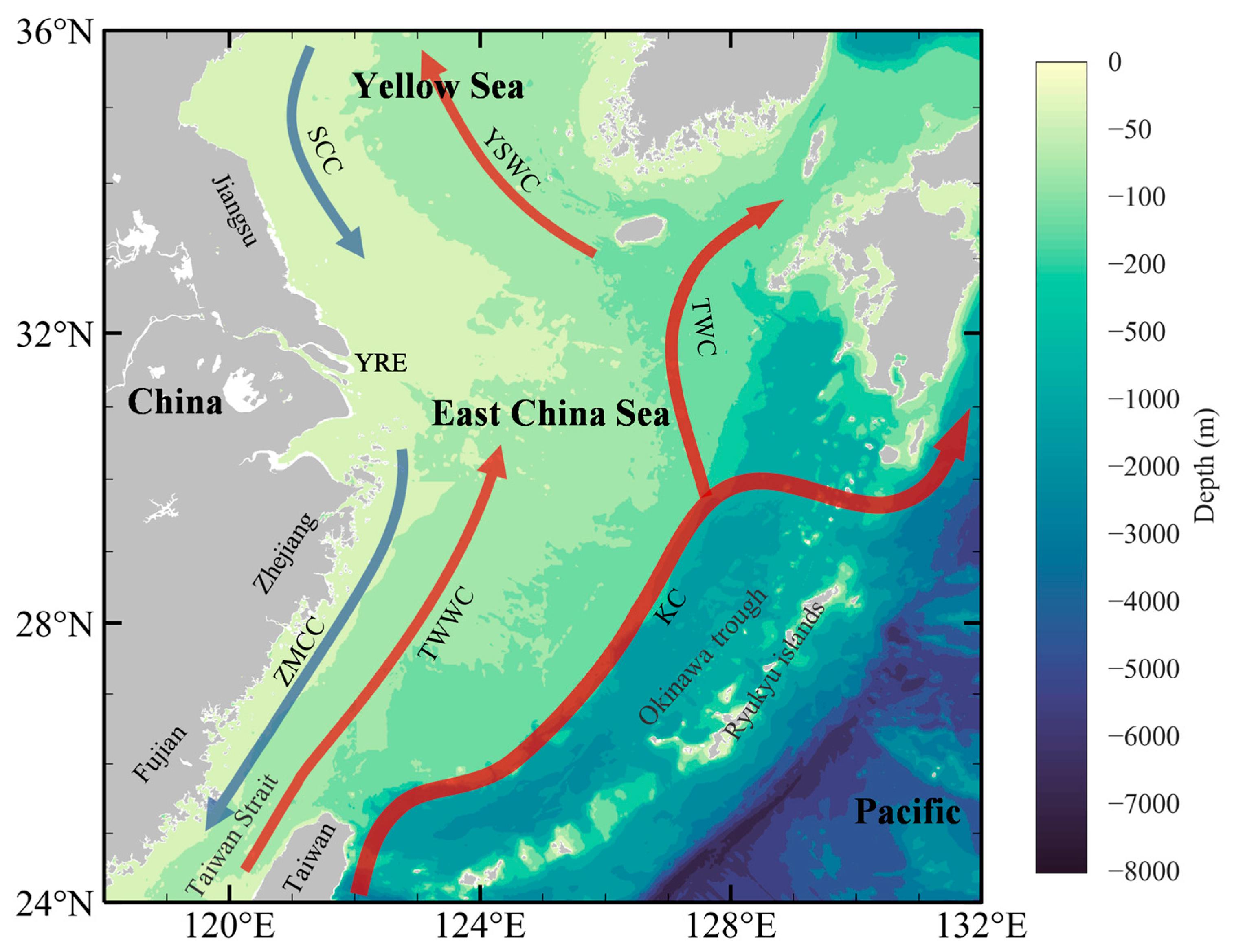
Figure 1. Map of the study area showing bathymetry and principal ocean currents.
Jmse 14 00054 g001
Figure 2. Overall architecture of the LSATrans-Net.
Jmse 14 00054 g002
Figure 3. Detailed architecture of LSATrans-Net.
Jmse 14 00054 g003
Figure 4. Encoder layer and Local Spatial Attention mechanism.
Jmse 14 00054 g004
Figure 5. Daily and average PCC comparison results of different models over a 7-Day forecast period (5% metric uncertainties).
Jmse 14 00054 g005
Figure 6. Daily and average RMSE comparison results of different models over a 7-Day forecast period (5% metric uncertainties).
Jmse 14 00054 g006
Figure 7. Spatial distribution of RMSE for different models across forecast days 1 to 7 (left to right). Four rows from top to bottom stand for the results from ConvLSTM, BiLSTM, CNN-Transformer, and LSATrans-Net, respectively. The black line denotes the −200 m isobath.
Jmse 14 00054 g007
Figure 8. Histograms of SLA prediction errors (units: m). The columns from left to right display the results for 1 to 7 forecast lead days; the rows from top to bottom present the forecast results for ConvLSTM, BiLSTM, CNN-Transformer, and LSATrans-Net, respectively.
Jmse 14 00054 g008
Figure 9. (a) RMSE and (b) MAE predicted by different models in 12 months.
Jmse 14 00054 g009
Figure 10. SLA forecast results over seven days under conventional weather conditions from February 1st to 7th, 2020. The first row represents satellite-observed actual SLA fields, the second row denotes model forecast SLA fields, and the third row represents forecast deviation by subtracting the observation from the prediction.
Jmse 14 00054 g010
Figure 11. Seven-day SLA forecast results during the passage of Super Typhoon Bavi (21–27 August 2020). The first row denotes satellite-observed actual SLA fields, the second row represents model forecast SLA fields, and the third row shows forecast deviation by subtracting the observation from the prediction.
Jmse 14 00054 g011
Figure 12. (a) RMSE and (b) MAE between the SLA-Forecast and ΔSLA-Forecast strategies over a 7-day forecast period.
Jmse 14 00054 g012
Figure 13. Spatial distribution of RMSE (units: m) for the SLA-Forecast (top) and ΔSLA-Forecast (middle) strategy over a 7-day forecast period (left to right), and the deviation between the above two strategies can be found at the bottom, subtracting the RMSE in the middle from the RMSE at the top. The black line denotes the −200 m isobath.
Jmse 14 00054 g013
Table 1. Hyperparameters and training settings of the LSATrans-Net.
DatasetTime Range
Input Dimension
Output Dimension
Train Split
Validation Split
Test Split
1993–2020
[1, 10, 48, 56]
[1, 7, 48, 56]
January 1993–December 2015
January 2016–December 2019
January 2020–December 2020
Model ArchitectureFeature Dimension
Number of Heads
Encoder Layers
Decoder Layers
Dropout
Spatial Radius
256
4
4
2
0.1
1
Training HyperparametersMax Epochs
Batch Size
Initial Learning Rate
Optimizer
Early Stopping Patience
100
16
5 × 10⁻⁵
ReduceLROnPlateau
10
Table 2. Daily and average MAE comparison results of different models over a 7-Day forecast (5% metric uncertainties).
Ahead/
Model Name
ConvLSTMBiLSTMCNN-TransformerLSATrans-Net
Day 10.00450 + 0.000060.00491 ± 0.000100.00498 ± 0.000140.00389 + 0.00011
Day 20.00845 ± 0.000120.01005 ± 0.000200.00872 + 0.000240.00754 ± 0.00021
Day 30.01222 ± 0.000160.01537 ± 0.000320.01136 + 0.000300.01128 ± 0.00028
Day 40.01605 + 0.000210.02071 ± 0.000440.01533 ± 0.000360.01327 ± 0.00032
Day 50.02006 ± 0.000280.02587 + 0.000570.01980 ± 0.000450.01509 ± 0.00032
Day 60.02430 + 0.000370.03069 ± 0.000690.02467 ± 0.000570.01754 + 0.00033
Day 70.02863 + 0.000490.03503 ± 0.000800.02983 ± 0.000700.02113 ± 0.00038
Average0.01632 ± 0.000230.02038 ± 0.000430.01638 ± 0.000330.01282 ± 0.00025
Disclaimer/Publisher’s Note: The statements, opinions and data contained in all publications are solely those of the individual author(s) and contributor(s) and not of MDPI and/or the editor(s). MDPI and/or the editor(s) disclaim responsibility for any injury to people or property resulting from any ideas, methods, instructions or products referred to in the content.