Article

Explainable Predictive Maintenance of Marine Engines Using a Hybrid BiLSTM-Attention-Kolmogorov Arnold Network

by
Alexandros S. Kalafatelis
1,*,
Georgios Levis
1,
Anastasios Giannopoulos
1,
Nikolaos Tsoulakos
2 and
Panagiotis Trakadas
1
1
Department of Port Management and Shipping, National and Kapodistrian University of Athens, 34400 Euboea, Greece
2
Laskaridis Shipping Co., Ltd., 14562 Athens, Greece
*
Author to whom correspondence should be addressed.
J. Mar. Sci. Eng. 2026, 14(1), 32; https://doi.org/10.3390/jmse14010032
Submission received: 7 December 2025 / Revised: 21 December 2025 / Accepted: 22 December 2025 / Published: 24 December 2025

Abstract

Predictive maintenance for marine engines requires forecasts that are both accurate and technically interpretable. This work introduces BEACON, a hybrid architecture that combines a bidirectional long short-term memory encoder with attention pooling, a Kolmogorov Arnold network and a lightweight multilayer perceptron for cylinder-level exhaust gas temperature forecasting, evaluated in both centralized and federated learning settings. On operational data from a bulk carrier, BEACON outperformed strong state-of-the-art baselines, achieving an RMSE of 0.5905 , MAE of 0.4713 and R 2 of approximately 0.95, while producing interpretable response curves and stable SHAP rankings across engine load regimes. A second contribution is the explicit evaluation of explanation stability in a federated learning setting, where BEACON maintained competitive accuracy and attained mean Spearman correlations above 0.8 between client-specific SHAP rankings, whereas baseline models exhibited substantially lower agreement. These results indicate that the proposed hybrid design provides an accurate and explanation-stable foundation for privacy-aware predictive maintenance of marine engines.

1. Introduction

The maritime sector accounts for close to 90% of global trade and is in the midst of a structural digital transition, often framed as “Shipping 4.0” and the “Internet of Ships” (IoS), where cyber-physical systems, dense sensor networks and ship-shore connectivity are gradually embedded into vessel operations [1,2,3]. In parallel, decarbonization policies, including the IMO GHG strategy targeting net-zero emissions by around 2050 [4], the extension of the EU Emissions Trading System (ETS) to maritime transport and the FuelEU Maritime regulation [5,6], are tightening constraints on fuel consumption, emissions and off-hire risk. Under these regulatory and economic pressures, the reliability and availability of the main propulsion systems are directly linked to both compliance and commercial performance.
Slow-speed two-stroke diesel and dual-fuel engines remain the dominant prime movers for deep-sea cargo ships, but their design and operating envelopes are evolving rapidly. Dual-fuel concepts (e.g., LNG/diesel), exhaust after-treatment and more advanced control schemes introduce additional operating modes, feedback loops and failure pathways, which complicate traditional experience-based maintenance strategies [7,8,9,10]. This has motivated a shift from fixed-interval or rule-based maintenance towards data-driven predictive maintenance (PdM) schemes that exploit high-frequency sensor streams [11,12]. Within the hierarchy of available measurements, exhaust gas temperature (EGT) is widely treated as a primary indicator for both main and auxiliary engines [13,14,15]. Cylinder- and manifold-level EGT reflects the combined influence of fuel injection, air-path dynamics, turbocharger performance and engine loading, and is routinely used in practice for condition assessment and alarm setting [14,15,16]. Accurate short-horizon forecasting of cylinder EGT is therefore a natural target for PdM frameworks aiming to support early warning, derating decisions and maintenance scheduling.
Traditional EGT modelling approaches based on grey-box formulations or kernel methods [17,18] have demonstrated useful performance, but often require extensive expert calibration and struggle to accommodate the full variability of real-world operations. Recent work has turned to deep learning (DL) models, in particular recurrent architectures such as long short-term memory (LSTM) and bidirectional LSTM networks (BiLSTM), which can exploit long-range temporal dependencies in multivariate sensor streams and have shown strong performance for marine engine fault warning and EGT prediction [10,15,19,20]. In most of these studies, however, the networks are treated as high-capacity black boxes, where they ingest large volumes of time-series data and output point forecasts or fault scores through opaque nonlinear transformations. In safety-critical maritime contexts, where predictions may trigger costly slowdowns, diversions, or manual inspections, the difficulty of explaining and linking model outputs to physically meaningful drivers remains a major barrier to adoption [12,21].
A second systemic challenge is data fragmentation. High-quality PdM models benefit from data that span different vessels, routes, ambient conditions, operating policies and fault types, yet sensor logs often remain siloed within individual shipowners, operators and OEMs due to commercial sensitivity, regulatory constraints and heterogeneous IT systems [22,23,24]. Centralizing raw engine data at scale is frequently infeasible or undesirable, especially when they are intertwined with cargo, routing and fuel strategies. Federated Learning (FL) has emerged as a natural candidate for such settings, as it enables multiple data owners to collaborate by exchanging model updates instead of raw data. Yet, standard FL algorithms such as FedAvg are known to degrade under strongly non-independent and non-identically distributed (Non-IID) data, leading to biased local models, client drift and fairness issues [25,26]. These issues are exacerbated when only a limited number of vessels participate, as is typical in early-stage maritime deployments.
Interpretability cuts across both centralized and federated settings. Existing maritime PdM work has started to integrate explainable AI (XAI) tools such as SHAP (Shapley Additive Explanations) to provide feature-level insights [12,21], but explanations are generally treated as post hoc overlays on otherwise opaque architectures. Furthermore, empirical studies in other domains have shown that explanations themselves can be unstable, where small changes in data, model initialization or optimization can induce shifts in feature attributions and saliency patterns even when predictive accuracy remains essentially unchanged [27,28]. Early work on FL combined with SHAP-based analyses indicates that Non-IID client data can alter both local and global attributions across sites [29,30], but this phenomenon has not yet been systematically studied for safety-critical maritime PdM, nor has it been examined jointly with model-internal functional structure.
To address these gaps, we propose BEACON, a hybrid BiLSTM-Attention-KAN-MLP architecture for cylinder-level EGT forecasting. The model combines a BiLSTM encoder, which extracts temporal features from multivariate engine time series, alongside an attention (Att) pooling mechanism and a Kolmogorov Arnold Network (KAN) block that replaces the opaque dense layers of a conventional BiLSTM with learnable univariate spline functions on its edges [31]. By appending a small MLP head for calibration, BEACON aims to preserve the sequence modelling strengths of deep recurrent networks while exposing a set of readable spline curves that can be inspected alongside SHAP-based attributions. Beyond the architecture itself, we analyze how SHAP feature rankings behave across federated clients under a fixed moderately non-IID Dirichlet partition, and we compare BEACON to state-of-the-art PdM baselines on both predictive and explanation stability metrics. Toward this direction, the main contributions of this work can be summarized as follows:
  • We introduce BEACON, a hybrid BiLSTM-Att-KAN-MLP architecture tailored to cylinder-level EGT forecasting for marine engines;
  • Using operational main engine data from a bulk carrier, we demonstrate that BEACON produces interpretable partial dependence curves built from the spline functions between latent features and EGT, consistent with known thermodynamic and operational relations, providing a “glass-box” view that complements SHAP-based feature attributions;
  • We benchmark BEACON against state-of-the-art PdM models in both centralized and federated settings under realistic moderate non-IID partitioning;
  • We study SHAP-based feature rankings across FL clients to show that explanation stability offers a complementary axis for comparing models in safety-critical applications such as in maritime maintenance (i.e., accuracy-interpretability trade-off).
The remainder of this paper is organized as follows. Section 2 reviews related work on maritime PdM and EGT modelling, KANs, XAI and FL. Section 3 details BEACON’s architecture. Section 4 describes the dataset, preprocessing pipeline and experimental setup. Section 5 reports results, including predictive performance and explanation stability analysis. Section 6 concludes the paper and outlines directions for future work.

2. Related Work

2.1. Maritime Predictive Maintenance and EGT Modelling

Within the broader landscape of PdM, several works have focused explicitly on EGT-based monitoring and forecasting. For instance, the work in [32] applies a nonlinear autoregressive exogenous model (NARX) neural network to forecast outlet EGT for an ME cylinder, showing that nonlinear autoregressive structures can capture temporal dependencies and support condition-based maintenance, though only tested using a relatively shallow architecture and a single-engine case study. Building on this direction, the work in [15] proposed a DL-based fault warning model that combines convolutional layers, BiLSTM and attention to predict EGT and trigger early warnings, demonstrating improved sensitivity to incipient ME faults on sea trial data. The work in [33] further investigated short-term EGT trend prediction using a BiLSTM enhanced with temporal pattern attention and a meta-heuristic optimizer for hyperparameter tuning, achieving high accuracy across different engine loads. In parallel, the work in [34] exploited cylinder and manifold EGT to diagnose piston-ring faults using an improved LSTM network, illustrating the diagnostic value of EGT for localized faults in the combustion chamber. At a higher level, PdM work has also addressed maintenance planning and logistics, for example through neural network-based repair rate estimation, linking predictive models to availability and resource constraints [35].
These studies collectively indicate that EGT is both a sensitive and practically accessible signal for engine health monitoring, and that recurrent model architectures are effective at extracting temporal patterns from multivariate engine data. However, existing approaches typically rely on fully connected dense heads with standard nonlinearities, treating the networks as opaque black boxes, and are trained in a centralized manner on data from a single vessel or under a homogeneous operating regime.

2.2. Kolmogorov Arnold Networks and Temporal Feature Extraction

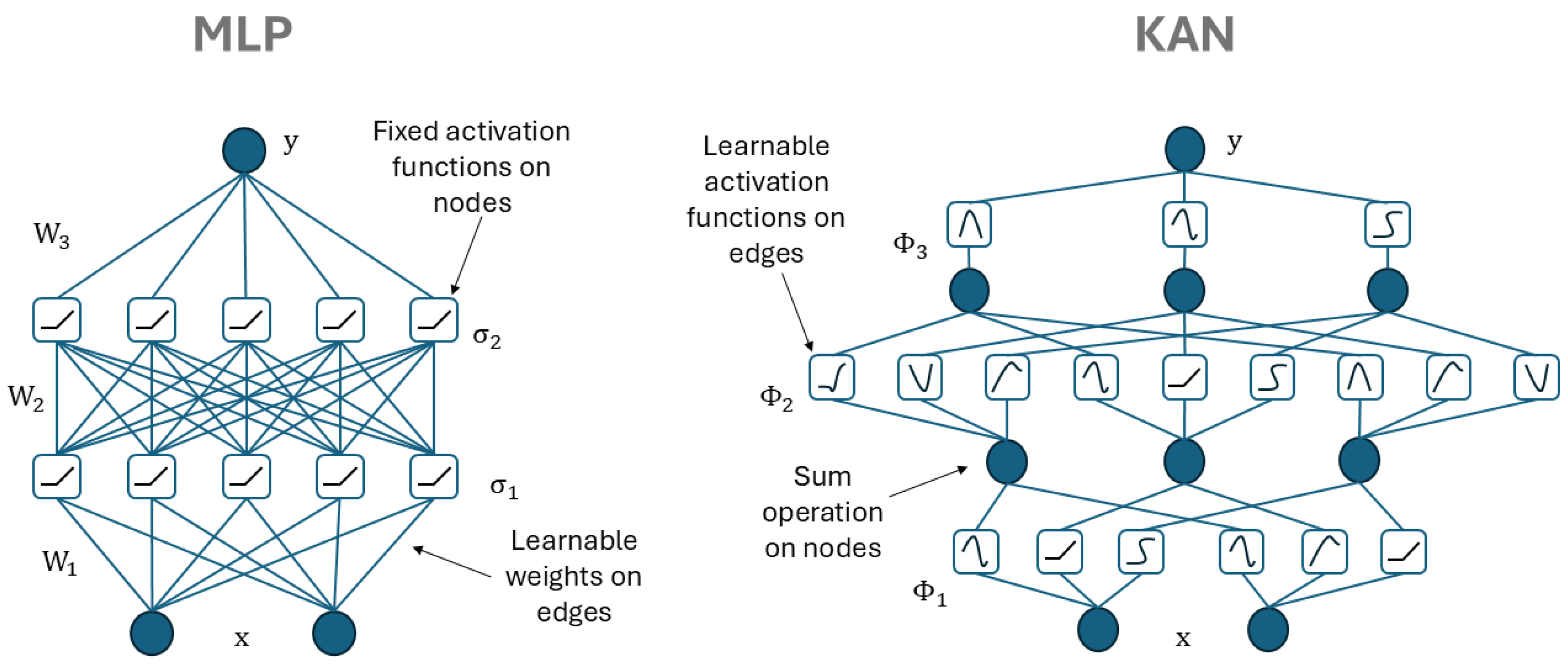
KANs have recently been proposed as an alternative to standard MLPs, replacing fixed activation functions with learnable univariate spline functions on each edge. The core idea is to exploit the Kolmogorov Arnold representation theorem to decompose multivariate mappings into compositions of low-dimensional functions with the spline parameters learned from data. This yields networks whose internal computations are more amenable to visualization and qualitative comparison with domain knowledge than those of standard dense layers [31].
Recent work has begun to adapt KAN-style function parameterizations to sequential learning, either by integrating recurrent memory into KAN blocks or by designing time-series-specific KAN variants for forecasting. For instance, the work in [36] applies KAN blocks to windowed time-series forecasting, reporting competitive or superior accuracy to MLP baselines on benchmark datasets and highlighting the readability of the learned spline functions for each lagged input. Similarly, the work in [37] proposes a KAN-based architecture tailored to temporal prediction, where historical observations are encoded as fixed-length vectors and passed through stacked KAN layers. In a related direction, temporal KAN (TKAN) [38] incorporates recurrent gating around KAN blocks, enabling the model to maintain a latent state that evolves with the sequence instead of relying only on fixed lag windows. As a result, temporal dependence is represented by the gating dynamics, while the KAN component continues to provide structured, spline-based mappings that are amenable to interpretation. Across these variants, temporal dependence is introduced either by explicit lag window construction or by lightweight recurrent/gating mechanisms that propagate a learned state over time, while the KAN blocks primarily replace conventional dense mappings with spline-parameterized transformations that are more amenable to inspection. However, despite this growing interest, there is limited work on combining high-capacity sequence encoders with KANs in a way that targets both long-range temporal dependencies and interpretable functional structure.

2.3. Explainable AI, Federated Learning and Explanation Stability

XAI has become a central theme in the broader machine learning literature, with feature attribution, surrogate modelling and example-based methods commonly used to probe black-box models. Foundational discussions such as in [39,40] emphasize the need to distinguish different notions of interpretability (e.g., transparency vs. post hoc explanations) and to align explanation methods with the underlying task and stakeholders. Critical studies such as [27,41] show that explanations can be sensitive to small perturbations of the model or data and, in extreme cases, fail simple sanity checks, motivating quantitative notions of explanation robustness and stability.
In the PdM context, XAI techniques have been applied to both remaining useful life (RUL) estimation and fault diagnosis for rotating machinery and other industrial assets. For maritime engines in particular, the work in [42] introduces an explainable anomaly detection framework that combines unsupervised models with SHAP to attribute abnormal behaviour to specific sensor channels, while the authors in [43] propose a time-series explanatory fault prediction scheme based on LSTM models and SHAP to highlight which parts of the input history drive a predicted fault event. These approaches, however, are developed in centralized settings and treat explanations as post hoc layers on top of otherwise opaque architectures.
From a deployment standpoint, the stability of such explanations is closely linked to operator trust and the appropriate use of AI-assisted maintenance recommendations. Studies in human–AI interaction show that explanation properties such as fidelity and internal consistency influence perceived understanding and trust, and that reliance behaviour cannot be explained by accuracy alone [44,45]. Within PdM, recent work further notes that explanations that fluctuate across runs or disagree across methods can undermine trustworthiness and complicate maintenance planning, motivating explicit criteria that account for explanation stability and agreement when models are used to support safety-critical decisions [46].
Recent FL work on monitoring and diagnosis has increasingly addressed system-level constraints that arise in real deployments. The study in [47] proposes an optimized adaptive FL updating scheme for collaborative diagnosis under label heterogeneity, with a focus on reducing redundant communication and improving robustness when clients have inconsistent label availability and uneven data quality. In a complementary direction, the work in [48] introduces a personalized federated fault diagnosis method based on a mixture of experts, allowing each client to retain specialized decision behaviour while still sharing a common representation. These contributions highlight the value of communication-aware updating and explicit personalization. In contrast, the present work focuses on continuous valued EGT forecasting for marine engines and quantifies cross-client stability of feature attributions, which is critical when explanations are used to justify maintenance actions across different vessels.
At the same time, there is a growing body of work at the intersection of XAI and FL. Classical FL algorithms such as FedAvg and their variants are now routinely applied, but explaining federated models is complicated by client heterogeneity and privacy constraints. The work in [49] studies the use of SHAP values to interpret federated models, while  [29] introduces DC-SHAP, a framework for distributing SHAP computations across privacy-preserving environments and aggregating them into consistent global explanations. Parallel to these developments, the works in [28,50] argue that explanation vectors themselves should be treated as objects of study, proposing metrics and aggregation schemes to characterize how attributions drift across training regimes, models and time.

2.4. Positioning of This Work

This study positions BEACON as a hybrid BiLSTM-Att-KAN-MLP architecture for cylinder-level EGT forecasting. The model is trained and evaluated in both centralized and federated setups, and its behaviour is analyzed jointly in terms of predictive accuracy, functional structure and quantitative measures of explanation stability across clients. Within maritime PdM, this work extends prior EGT forecasting studies by moving from opaque dense heads to interpretable analysis using SHAP analysis and partial dependence curves extracted directly from the KAN block. In the FL setting, BEACON is benchmarked against representative state-of-the-art PdM baselines under a realistic moderately non-IID partition, and we explicitly track how SHAP-based feature rankings vary across clients. To the best of our knowledge, this is the first study that examines architectures along both predictive and explanation stability axes under federated training, with a view toward supporting maintenance decisions.

3. Model Architecture

This section describes the BEACON architecture for sequence to scalar EGT prediction. We first formalize the supervised learning setup and notation, then present the bidirectional LSTM (BiLSTM) encoder, the deterministic attention pooling mechanism, the KAN block and the residual regression head. We then define the training objective and summarize the forward and training procedures. A high-level illustration of BEACON is given in Figure 1.

3.1. Problem Setup and Notation

At each decision time index t, the input to the model is a multivariate time window
X t = x t T + 1 , , x t R T × d
where x τ R d is the feature vector at time τ , T is the number of historical time steps in the window and d is the number of input features such as engine load, revolution rate and temperatures. The one-step-ahead prediction target is the scalar EGT
y t + 1 R
All input features are standardized feature-wise using their training set mean μ j and standard deviation σ j , whereas the target is standardized using its mean μ y and standard deviation σ y . We denote the BEACON mapping by
f θ : R T × d R
where θ collects all trainable parameters and f θ ( X t ) outputs a standardized EGT prediction y ^ t + 1 . The corresponding physical EGT prediction is
y ˜ t + 1 = μ y + σ y y ^ t + 1
where μ y R and σ y > 0 denote the target mean and standard deviation estimated from the training set and y ˜ t + 1 is expressed in degrees Celsius.

3.2. Temporal Bidirectional LSTM Encoder

We first encode each input window X t = [ x t T + 1 , , x t ] using a stack of L bidirectional LSTM layers. Within each window, we reindex for convenience as X = [ x 1 , , x T ] , where x τ R d and τ { 1 , , T } . For layer { 1 , , L } and time index τ , the forward and backward LSTM cells update their hidden and cell states as
h , τ , c , τ = LSTM fwd u , τ , h , τ 1 , c , τ 1 ,
h , τ , c , τ = LSTM bwd u , τ , h , τ + 1 , c , τ + 1
where u 1 , τ = x τ is the input at time τ for the first layer; u , τ = h 1 , τ for > 1 is the output of the previous BiLSTM layer at time τ ; h , τ , h , τ R h are the forward and backward hidden states at layer and time τ ; c , τ , c , τ R h are the corresponding cell states; and LSTM fwd ( · ) and LSTM bwd ( · ) denote standard LSTM cells parameterized at layer .
Each unidirectional LSTM cell follows the usual gating equations. For the forward cell of layer , we have
i , τ = σ W i ( ) u , τ + U i ( ) h , τ 1 + b i ( ) , f , τ = σ W f ( ) u , τ + U f ( ) h , τ 1 + b f ( ) , o , τ = σ W o ( ) u , τ + U o ( ) h , τ 1 + b o ( ) , c ˜ , τ = tanh W c ( ) u , τ + U c ( ) h , τ 1 + b c ( ) , c , τ = f , τ c , τ 1 + i , τ c ˜ , τ , h , τ = o , τ tanh c , τ
where i , τ , f , τ , o , τ R h are the input, forget and output gates; c ˜ , τ R h is the candidate cell state; W { · } ( ) R h × d and U { · } ( ) R h × h are trainable weight matrices; b { · } ( ) R h are trainable bias vectors; σ ( · ) denotes the logistic sigmoid; tanh ( · ) is the hyperbolic tangent; and ⊙ denotes element-wise multiplication. Here, d 1 = d for the first layer, and d = 2 h for > 1 . The backward LSTM cell uses analogous equations with h , τ + 1 and c , τ + 1 as recurrent states. Furthermore, the bidirectional hidden state at layer and time τ is formed by concatenation of the forward and backward states
h , τ = h , τ h , τ R 2 h
where 2 h is the total hidden dimensionality per time step at that layer. The outputs of the top layer across time yields is collected as follows:
H L = [ h L , 1 , , h L , T ] R T × 2 h
where each row corresponds to a position τ within the window and each column corresponds to one of the 2 h concatenated forward and backward features. For a mini batch of size B, H L generalizes to a tensor in R B × T × 2 h .

3.3. Deterministic Attention Pooling

To aggregate information across the T encoded time steps into a fixed dimension vector, we apply a deterministic soft attention mechanism. Given H L , an attention score e τ is computed for each time step as follows:
e τ = v a tanh W a h L , τ + b a
where W a R r × 2 h is a trainable weight matrix, b a R r is a bias vector, v a R r is a trainable vector, r is the attention hidden size and tanh ( · ) is applied element-wise. The normalized attention weights are given by
α τ = exp ( e τ ) k = 1 T exp ( e k ) , τ = 1 , , T
where α τ ( 0 , 1 ) and τ = 1 T α τ = 1 , while the attention-pooled context vector is
c = τ = 1 T α τ h L , τ R 2 h
where c aggregates the BiLSTM features over time, weighted by their learned relevance α τ . To form the input to the KAN block, we further concatenate c with the following additional summary features:
z ( 0 ) = c , x T , ϕ ( X ) R m
where x T R d is the standardized feature vector at the last time step, ϕ ( X ) denotes optional handcrafted temporal aggregates such as moving averages and m is the resulting concatenated dimensionality. In the main configuration, ϕ ( · ) is omitted and z ( 0 ) reduces to the concatenation of c and x T .

3.4. Kolmogorov Arnold Network

3.4.1. Comparison with a Multilayer Perceptron

Before describing their implementation in BEACON, it is useful to contrast KANs with a standard MLP. Let z R m denote an input vector. Specifically, a single hidden-layer MLP computes
MLP ( z ) = W ( 2 ) σ W ( 1 ) z + b ( 1 ) + b ( 2 )
where W ( 1 ) R H × m and W ( 2 ) R 1 × H are weight matrices, b ( 1 ) R H and b ( 2 ) R are bias terms, H is the hidden width and σ ( · ) is a point-wise nonlinearity. The first layer mixes all coordinates of z linearly before applying σ ( · ) .
In contrast, a KAN follows a Kolmogorov Arnold style representation and uses univariate functions on each coordinate before aggregation. For an input z = ( z 1 , , z m ) , a KAN style mapping can be written as
f ( z ) = q = 1 Q g q r = 1 m ϕ r , q ( z r )
where ϕ r , q : R R are learnable univariate inner functions, g q : R R are outer univariate functions, Q is the number of inner channels and the indices r and q enumerate input coordinates and channels. Each coordinate is first transformed by a family of univariate maps and only then combined across dimensions.
In a conventional MLP, the nonlinearity is fixed in advance, for example a rectified linear unit or hyperbolic tangent, and learning proceeds by adapting the weight matrices and biases. In a KAN, the univariate functions ϕ r , q and g q play the role of data-driven activation functions that are parameterized for instance by spline coefficients, while the linear mixing stage that follows remains relatively simple. This ordering gives KANs a separable-per-coordinate inductive bias and improves interpretability. The functions ϕ r , q can be further plotted against their input arguments, which reveals thresholds, saturation effects and other one-dimensional response patterns. The architectural difference between the two models is showcased in Figure 2.

3.4.2. B-Spline Basis for 1D Functions

In BEACON, the KAN block approximates smooth multivariate response surfaces using compositions and sums of univariate spline functions, following the Kolmogorov Arnold representation theorem. Let a scalar input u R be affinely normalized into an interval [ u ̲ , u ¯ ] , and let { B k ( u ) } k = 1 K denote a B-spline basis of order q defined on a knot sequence { κ j } . Any smooth univariate function g : R R in the span of this basis can be written as
g ( u ) = k = 1 K w k B k ( u )
where w k R are learnable coefficients, K is the number of basis functions and the choice of knot sequence { κ j } and order q determines the smoothness and support of the basis functions. The expressions above describe the canonical B-spline component of the KAN. In BEACON, we further augment this basis with two additional learnable channels, a Swish term and a sinusoidal term, so that the effective per-input basis vector is
b ˜ ( u ) = B 1 ( u ) , , B K ( u ) , swish ( u ) , sin ( u )
where swish ( u ) = u σ ( u ) .

3.4.3. Single KAN Layer

Consider a KAN layer indexed by with input z ( 1 ) R m 1 , which contains m 1 scalar channels. For each input dimension j { 1 , , m 1 } , we evaluate the extended basis on z j ( 1 ) :
b ˜ j z j ( 1 ) = b ˜ z j ( 1 ) R K + 2
where b ˜ ( · ) is defined in (17). Concatenating the basis expansions across all input dimensions yields
b ( ) = b ˜ 1 , , b ˜ m 1 R m 1 ( K + 2 ) .
In its canonical form, a KAN layer applies a linear map followed by a point-wise nonlinearity. In BEACON, we add a simple quadratic lifting before this linear mixing. Specifically, we form
b ^ ( ) = b ( ) , b ( ) b ( )
where ⊙ denotes element-wise multiplication. The hidden representation at layer is then represented as
z ( ) = ρ W ( ) b ^ ( ) + b 0 ( )
where W ( ) and b 0 ( ) are trainable parameters and ρ ( · ) is an element-wise activation (e.g., tanh). When the quadratic lifting and auxiliary channels are omitted, (21) reduces to the canonical B-spline KAN described earlier. Furthermore, in BEACON, we use L KAN = 3 KAN layers with width p, so that
z ( 1 ) = KANLayer 1 z ( 0 ) , z ( 2 ) = KANLayer 2 z ( 1 ) , z ( 3 ) = KANLayer 3 z ( 2 )
and the final KAN representation is z ( 3 ) . This output is passed to a shallow linear head that predicts a standardized residual
y ^ t + 1 ( KAN ) = w r z ( D ) + b r
where w r and b r are trainable parameters.

3.5. Training Objective

Let D = { ( X t ( i ) , y t + 1 ( i ) , y t ( i ) , meas ) } i = 1 N denote the training set of N windows, one-step-ahead targets and baseline EGTs. The standardized ground truth for each sample is
y ^ t + 1 ( i ) , true = y t + 1 ( i ) μ y σ y
where y t + 1 ( i ) is the physical EGT for sample i using the mean squared error (MSE) on standardized targets L ( θ ) .
In addition, to discourage overly oscillatory spline functions, we further regularize the differences between adjacent B-spline coefficients. Let w , j R K denote the coefficient vector associated with the jth scalar input at KAN layer , and let D diff R ( K 1 ) × K be a discrete first- or second-order difference operator. The spline regularization term is
R spline = = 1 L KAN j D diff w , j 2 2
where the inner sum runs over all scalar inputs to layer , and · 2 denotes the Euclidean norm. Additionally, the additional Swish and sinusoidal channels in the implementation are included in θ KAN but are not penalized by R spline , thus making the total training objective
J ( θ ) = L ( θ ) + λ spl R spline
where λ spl 0 controls the strength of the spline smoothing. The model is trained using mini batch stochastic gradient descent with Adam, as well as backpropagation through time for the BiLSTM and standard backpropagation for the KAN block and regression head. Algorithms 1 and 2 summarize the BEACON inference and training procedures.
Algorithm 1 BEACON forward pass for a single window
Require: 
Historical window X t R T × d , parameters θ = { θ BiLSTM , θ att , θ KAN , θ head } , standardization statistics { μ j , σ j } j = 1 d and μ y , σ y , residual weight λ res
Ensure: 
Predicted EGT y ˜ t + 1 in physical units
1:
Standardize features: x τ , j ( x τ , j μ j ) / σ j for all τ and j
2:
Standardize baseline: y ^ t meas ( y t meas μ y ) / σ y
3:
BiLSTM encoding: H L BiLSTM θ BiLSTM ( X t )
4:
Attention pooling: compute e τ via (10), α τ via (11), and c via (12)
5:
Form KAN input: z ( 0 ) [ c , x T , ϕ ( X t ) ]
6:
for = 1 to L KAN  do
7:
    compute b ( ) ^ via (17), (19) and (20)
8:
     z ( ) ρ ( W ( ) b ^ ( ) + b 0 ( ) )
9:
end for
10:
KAN regression: y ^ t + 1 ( KAN ) w r z ( D ) + b r
11:
Residual link: y ^ t + 1 y ^ t meas + λ res y ^ t + 1 ( KAN )
12:
Destandardize: y ˜ t + 1 μ y + σ y y ^ t + 1
13:
return y ˜ t + 1
Algorithm 2 BEACON training with mini batch SGD and spline regularization
Require: 
Training set D = { ( X t ( i ) , y t + 1 ( i ) , y t ( i ) , meas ) } i = 1 N , statistics { μ j , σ j } j = 1 d and μ y , σ y , initial parameters θ , batch size B, number of epochs E, learning rate η , spline weight λ spl , optimizer (Adam)
Ensure: 
Trained parameters θ
1:
for  e = 1 to E do
2:
    shuffle D and split into mini batches { B }
3:
    for each mini batch B of size B do
4:
        standardize features and targets in B using { μ j , σ j } and (24)
5:
        for each sample in B , compute y ^ t + 1 ( i ) via Algorithm 1
6:
        compute L ( θ ) and R spline via (25)
7:
         J L ( θ ) + λ spl R spline
8:
        backpropagate θ J and update θ with Adam
9:
    end for
10:
end for
11:
return  θ θ

4. Experimental Setup

All experiments were executed on a dedicated server equipped with an AMD EPYC 7402 CPU with 24 cores and 48 threads, 128 GB of RAM and a single NVIDIA L40s GPU, running Ubuntu 22.04.5 LTS. The models were implemented in Python 3.11.0, using PyTorch 2.0.0, TensorFlow 2.13.0 (for TKAN) and Flower 1.6.0 to orchestrate the FL experiments, while GPU acceleration was used for all training runs.

4.1. Dataset

For the development and evaluation of BEACON, we used an extended version of the dataset introduced in [51]. The operational data were collected from a bulk carrier operated by Laskaridis Shipping Co., equipped with a low-speed diesel ME rated at 12,009 HP and with a deadweight tonnage of 75,618 DWT. The dataset comprises high-frequency time series from 759 sensors distributed across the vessel, covering engine performance, fuel system variables, air and cooling circuits, and auxiliary subsystems.
The prediction target in this study is the ME cylinder EGT of Cylinder 1, expressed in degrees Celsius (°C). This temperature is measured at the cylinder exhaust outlet and is routinely used as a diagnostic indicator for misfires, imbalance between cylinders and abnormal combustion [15,52]. We focus on Cylinder 1 because its EGT is consistently available in the dataset and representative of the thermal behaviour of the engine. From the full set of 759 channels we retain a subset of physically meaningful variables that are directly related to engine loading, air path, fuel delivery and cooling conditions. These features, together with past values of Cylinder 1 EGT, form the input to all models. The selected drivers are summarized in Table 1.

4.2. Data Preprocessing and Feature Engineering

We first computed Pearson correlation coefficients r i between each candidate predictor X i and the target variable, the standardized Cylinder 1 EGT. Predictors with absolute correlation | r i | > 0.5 were retained, which corresponds to a large effect size in the sense of Cohen [53]. In parallel, feature selection was also constrained by domain knowledge, prioritizing variables with established causal relevance to EGT. This screening step yielded a final set of twelve variables that are also interpretable from an engine physics standpoint and originate from the main propulsion engine and its supporting subsystems (air path, fuel delivery and cooling circuits), which jointly determine cylinder thermal behavior. The retained features are reported in Table 1. All retained variables and the target were then standardized using z score normalization, with statistics computed on the training set.
Missing values in the multivariate time series were handled in two stages. For each channel, internal gaps were first filled by forward filling, where the last observed value is propagated forward in time until a new observation appears. Any remaining missing entries at the beginning of a series were then filled by backward filling, using the first available future observation in order to preserve temporal coherence. Samples with missing EGT targets were removed from the dataset. For quality control, scatter plots of each retained predictor against the target were inspected to confirm approximate monotonic relationships and to flag obvious outliers.
All models were trained on fixed-length windows of standardized multivariate sequences. Past EGT values are included directly in the input sequence, which provides an autoregressive history without constructing separate lagged features. Let D denote the number of retained variables including EGT. For each starting index i, we construct an input sequence X i R 48 × D , which contains the previous 48 time steps of all normalized variables over times [ i , , i + 47 ] , as well as a scalar target y i equal to the normalized EGT at time i + 48 . This corresponds to a one-step-ahead forecast relative to the end of the window. The resulting sequence dataset is split into training, validation and test subsets with a ratio of 70%/15%/15%. All validation and test samples occur strictly after the training samples in time.

4.3. Baseline PdM Models, Training Setup and Evaluation Metrics

4.3.1. Baseline Predictive Models

We benchmark the proposed BEACON architecture against four representative PdM baselines. These are a BiLSTM variant, a temporal Kolmogorov Arnold Network model (TKAN) based on [38], an IBWO LSTM tuned by evolutionary search as in [34] and a nonlinear autoregressive model with exogenous inputs (NARX) [32]. All the sequence models operate on the same input window length of 48 time steps and predict the same one-step-ahead EGT target.
The model architectures and hyperparameters were selected by validation-guided tuning on the operational dataset. In detail, BEACON consists of a two-layer BiLSTM encoder with 352 hidden units per direction and a dropout probability of 0.03 between stacked layers. The encoder output is passed through deterministic attention pooling, as described in Section 3.3, to obtain a fixed dimensional context vector. This context, concatenated with the last standardized input vector, is fed into a KAN block of depth three and width 320. Each KAN layer uses cubic B-spline-basis functions with grid size 12, which yields K = 15 basis functions per input dimension. The univariate channels combine B-spline, Swish and sinusoidal components, and their outputs are mixed through a quadratic combination with a dropout rate of 0.05 applied inside the block. The KAN output is mapped to a scalar residual by a linear head, which is added to a scaled version of the measured baseline EGT through a residual link with fixed weight λ r e s = 0.5 . This configuration was chosen to balance predictive accuracy, stability of the learned functional mappings and computational cost, and is intended as a strong and reproducible operating point rather than a globally optimal setting. The BiLSTM baseline shares the same recurrent encoder and attention-based aggregation as BEACON but replaces the KAN block with a standard fully connected regression head. The IBWO LSTM baseline follows the architecture in [34]. It is implemented as a two-layer unidirectional LSTM with hidden size 128 and dropout 0.2. The regression head takes the last hidden state concatenated with the last input vector and outputs a sequence-to-one prediction at the final time step. In centralized experiments, the Improved Binary Whale Optimization algorithm is used to tune LSTM hyperparameters. In FL experiments, we fix the architecture and train it with standard gradient-based optimization on each client without an on-device evolutionary search. The TKAN baseline is based on the temporal KAN formulation of [38]. The hidden dimensionality is set to 128 and the sequence length is fixed at 48. The prediction head includes the last raw time step through a residual connection and outputs a scalar forecast of EGT. Finally, the NARX model is a classical nonlinear autoregressive model with exogenous inputs. The target output is scalar EGT, while the exogenous input dimensionality is equal to the number of predictors excluding EGT. The model uses 20 lags of the target, 25 lags of the exogenous covariates and a hidden layer of size 64 and dropout probability 0.2.
All models are trained with the Adam optimizer with learning rate 1 × 10 3 and weight decay 1 × 10 5 . The loss function is the mean squared error between the predicted and measured EGT. To improve stability in the presence of occasional outliers, gradients are clipped so that their 2 norm does not exceed 1. For the DL models (BEACON, BiLSTM-Att-MLP, IBWO LSTM and TKAN), the batch size is set to 64, while for NARX, which has a smaller parameter count, a batch size of 128 is used.

4.3.2. Federated Learning Setup

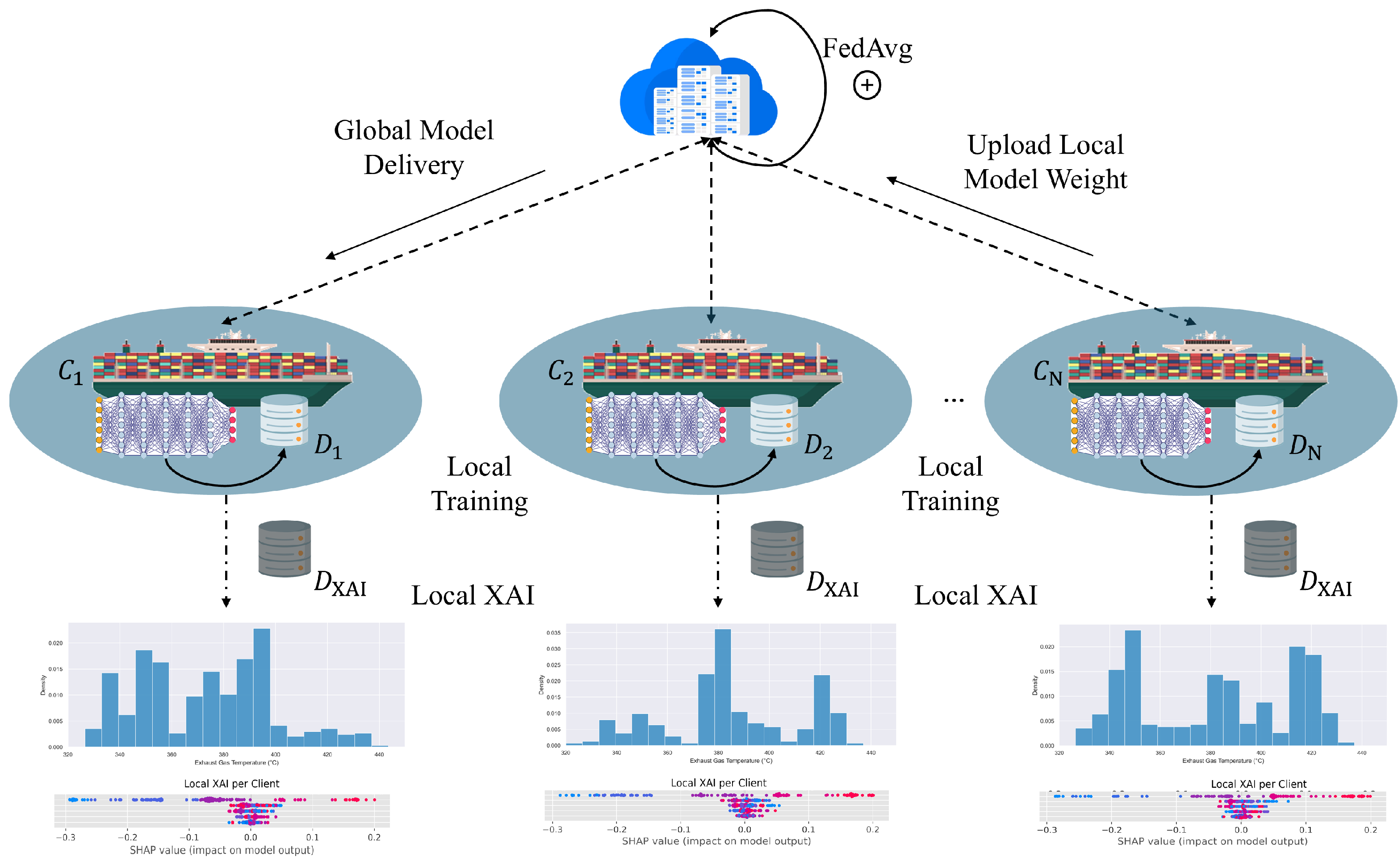
For the FL experiments, we adopt a setting with five synchronous clients and a single central coordinator. Each client represents a vessel-specific or regime-specific partition of the full dataset. Furthermore, before forming client datasets, we first separate a fixed 10 % chronological tail of the sequence data. This subset is never used for training and serves as a common evaluation set for all clients when computing XAI stability metrics across FL clients. The remaining 90 % of the data are used for FL training and validation. Within this 90 % , each client’s local portion is obtained by sampling from a Dirichlet distribution over sample indices with concentration parameter α = 1.0 , following the protocol in [54]. This yields moderately heterogeneous but not pathologically skewed client datasets, which we regard as representative of pragmatic moderately non-IID conditions in fleets with similar ME designs and maintenance policies. For each client, the local data are then split chronologically into training, validation and test subsets using the same 70 % / 15 % / 15 % ratio as in the centralized setting. All federated experiments use FedAvg [25] as the aggregation rule. No server-side momentum or adaptive optimization is applied in the aggregation step and no client dropouts are simulated. We acknowledge that FedAvg can degrade under non-IID client data, but in this work, it serves as a widely adopted baseline so that observed differences in accuracy and explanation stability can be attributed primarily to the model architecture rather than to specialized aggregation schemes.
On each client, local training uses the Adam optimizer with learning rate 1 × 10 4 . Each round performs on five local epochs with the same batch sizes as in the centralized experiments. Gradients are clipped to an 2 norm of 1.0 to stabilize training in the presence of occasional outliers. All experiments run for 20 communication rounds and all five clients participate in every round for both training and evaluation. To mimic a realistic deployment and to reduce the number of communication rounds required for convergence, each federated run is warm-started from the corresponding centrally trained model rather than using random initialization. Figure 3 illustrates the overall FL setup used in this study.

4.3.3. Evaluation Metrics

For each evaluation, we report across five random seeds standard regression metrics, namely the root mean square error (RMSE), mean absolute error (MAE) and coefficient of determination ( R 2 ), together with a measure of model cost given by the number of trainable parameters:
RMSE = 1 N i = 1 N y ^ i y i 2 .
MAE = 1 N i = 1 N y ^ i y i .
R 2 = 1 i = 1 N y ^ i y i 2 i = 1 N y i y ¯ 2 , y ¯ = 1 N i = 1 N y i ,
where y ¯ is the sample mean of the measured EGT. Furthermore, to assess centralized explainability and cross-client explanation stability in the FL setup, we also quantify the agreement between SHAP-based feature rankings, using the SHAP GradientExplainer, across participating clients [55]. Let M denote the number of features and let s ( a ) = ( s 1 ( a ) , , s M ( a ) ) and s ( b ) = ( s 1 ( b ) , , s M ( b ) ) be two vectors of global importance scores obtained from SHAP for two configurations such as different α values or different clients. We convert these scores to ranks r j ( a ) and r j ( b ) for j = 1 , , M . The Spearman rank correlation between the two rankings is defined as
ρ S = 1 6 j = 1 M r j ( a ) r j ( b ) 2 M M 2 1 .
The Kendall rank correlation is defined as
τ k = N c N d M 2 ,
where N c is the number of concordant feature pairs and N d is the number of discordant feature pairs between the two rankings. Finally, to capture agreement in the most influential features, we compute the Jaccard index at rank five. Let A ( a ) and A ( b ) denote the sets of the top five features in the two rankings. The Jaccard index at five is
J @ 5 = A ( a ) A ( b ) A ( a ) A ( b ) .
For each pair of configurations, we report the average Spearman and Kendall correlations and the average J @ 5 . These metrics provide a compact summary of explanation stability under different non-independent and non-identically distributed regimes.

5. Results

5.1. Centralized Performance Evaluation

Table 2 summarizes the centralized performance of BEACON and the baseline predictive maintenance models. All DL model architectures except IBWO-LSTM reach a coefficient of determination above 0.93 , which confirms that Cylinder 1 EGT is a highly predictable signal when the ME operating variables are available. Furthermore, BEACON attains the lowest errors among all models. Its RMSE of 0.5905 and MAE of 0.4713 correspond to relative reductions of approximately 16 % with respect to the BiLSTM baseline in both metrics. The improvement is even larger when compared with TKAN and IBWO–LSTM, where the average RMSE nearly doubles. The gain in R 2 is smaller in absolute terms, from 0.9473 for BiLSTM to 0.9496 for BEACON, but the standard deviations indicate that this difference is consistent across runs.
The dispersion across seeds is also informative concerning predictive stability. BEACON and BiLSTM exhibit small standard deviations in both their RMSE and MAE, which points to stable convergence under the chosen training protocol. In contrast, IBWO-LSTM ( 0.19 ) and NARX ( 0.23 ) show markedly higher variability, reflecting potentially less reliable performance in practice. TKAN lies between these extremes, with mean errors higher than BiLSTM and BEACON and moderate variability. The classical NARX model is clearly outperformed by all the DL-based approaches. Its mean RMSE and MAE are more than twice as high as those of BEACON, and its R 2 drops to 0.80 on average. This result underlines the advantage of learning nonlinear temporal representations directly from multivariate sensor histories instead of relying on fixed lag structures and manual feature selection.
In terms of model size, BEACON has approximately 7.9 million trainable parameters, which is about twice the parameter count of BiLSTM. IBWO-LSTM and TKAN are substantially more compact, with 0.28 and 0.35 million parameters, respectively, while NARX has the smallest footprint. Although these lighter models are attractive from a storage perspective, their error levels and variability indicate that they provide weaker predictive performance for the EGT forecasting task considered here.
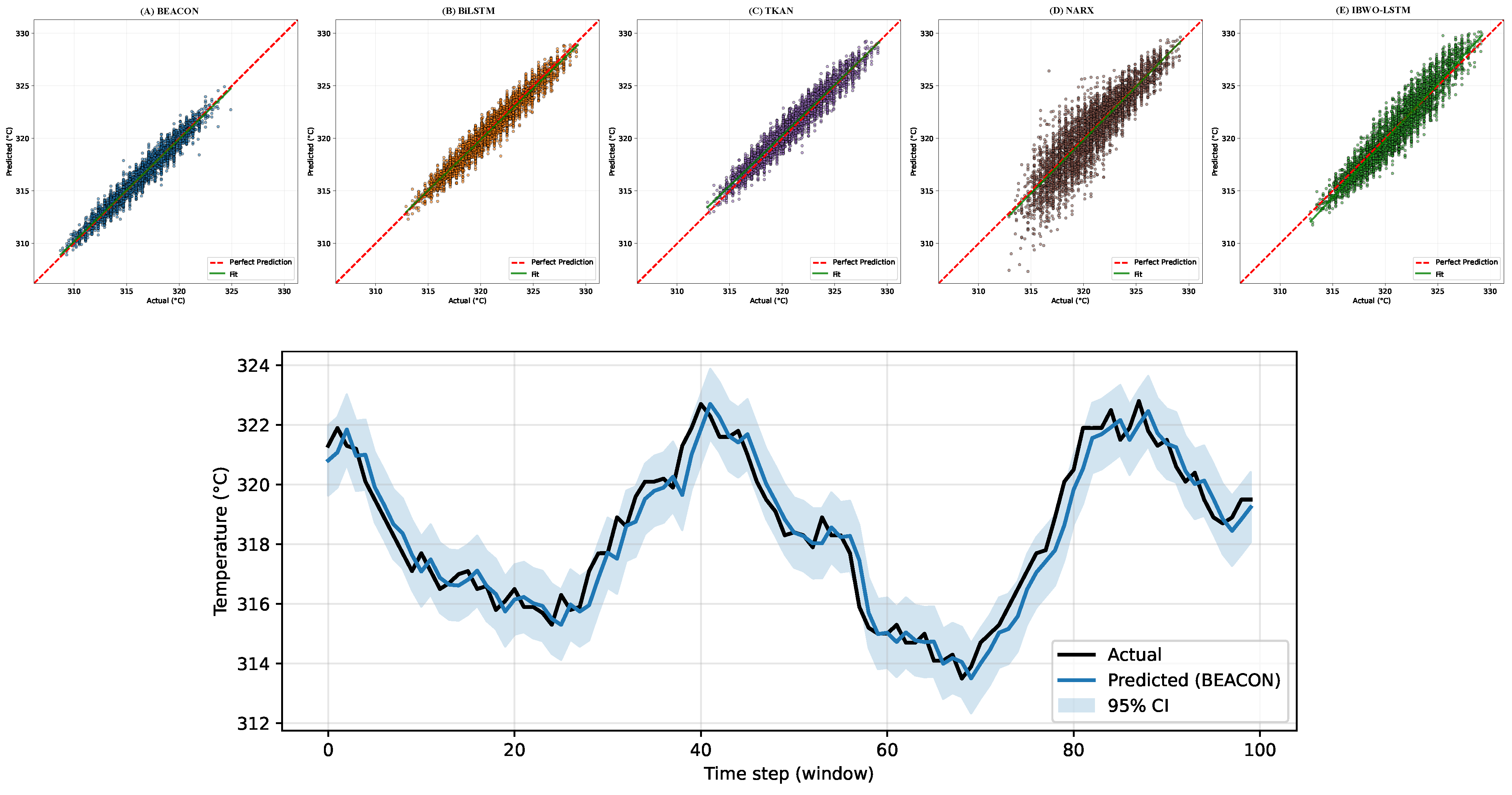
Figure 4 provides a complementary view of the centralized results in Table 2. In the top panel, BEACON produces a compact cloud of points that lies very close to the identity line across the full EGT range, and the fitted regression line is almost indistinguishable from perfect calibration. The BiLSTM and TKAN models follow the same general trend but exhibit visibly larger vertical spread, especially at higher temperatures, which reflects their higher RMSE and MAE. The NARX and IBWO-LSTM baselines show the widest scatter and a more pronounced tilt of the fitted line, indicating a combination of larger variance and systematic bias. Taken together, the scatter plots confirm that BEACON achieves the most accurate and best calibrated point-wise predictions among the evaluated models. Furthermore, the bottom panel of Figure 4 shows a representative validation segment for Cylinder 1 EGT together with the BEACON forecast and its confidence band. Specifically, over this 100-step horizon sample, the model is shown to track short-term fluctuations effectively, while the uncertainty band remains relatively narrow. Deviations between measured and predicted temperatures stay within a small fraction of °C. This behaviour is consistent with the error metrics in Table 2.
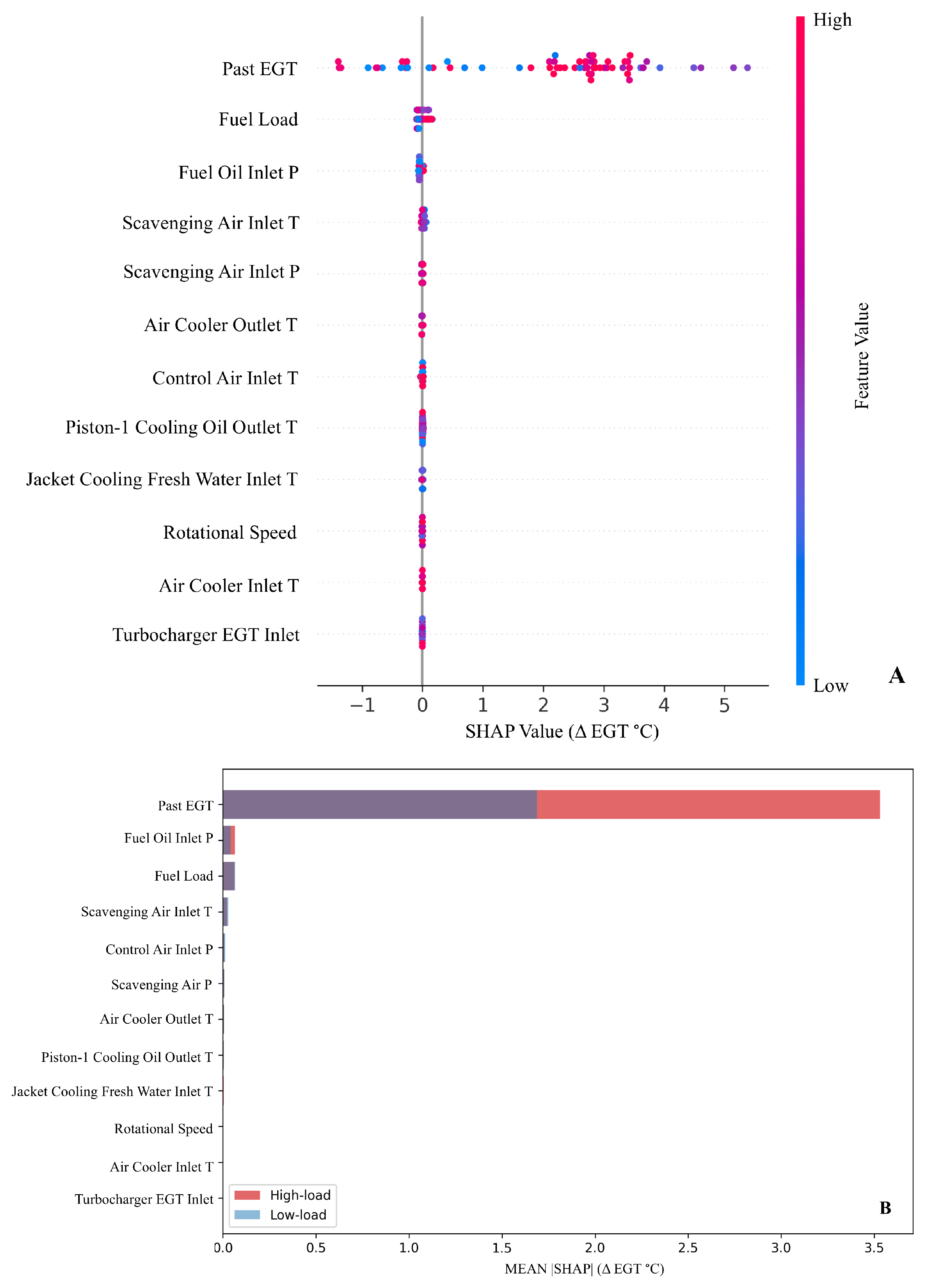
Figure 5A shows the global SHAP distribution for BEACON on the validation set. The horizontal axis gives the contribution of each feature to the predicted Cylinder EGT, while colour indicates whether the underlying feature value is low or high. Past EGT clearly dominates the ranking. Its contributions extend from values close to 0 up to roughly 5 ° C , and high recent temperatures are consistently associated with positive SHAP values, which is consistent with the strong temporal persistence of exhaust temperature. Fuel load emerges as the second most influential driver. High load values shift the prediction toward a higher EGT, whereas low loads produce small negative or near-zero contributions. The remaining variables, such as fuel oil inlet pressure, scavenge air temperature and pressure, air cooler temperatures, jacket cooling water inlet temperature and rotational speed, form tight bands around zero. Their colour patterns remain physically coherent, but their magnitudes are an order of magnitude smaller than those of past EGT and fuel load, which indicates that they act mainly as fine corrections rather than primary predictors.
The regime-wise analysis in Figure 5B examines whether the model relies on different inputs at low and high load. In both regimes, past EGT accounts for the majority of the attribution mass, with mean absolute contributions around 3.5 ° C and very similar values for low-load and high-load data. All other features exhibit mean absolute SHAP values below approximately 0.1 ° C across regimes. Fuel oil inlet pressure and fuel load have the largest of these secondary effects, yet their impact remains small compared with past EGT. The ranking is therefore highly stable, as BEACON does not switch to a different set of predictors in the high-load regime, but instead modulates the strength of the same physically meaningful variables.
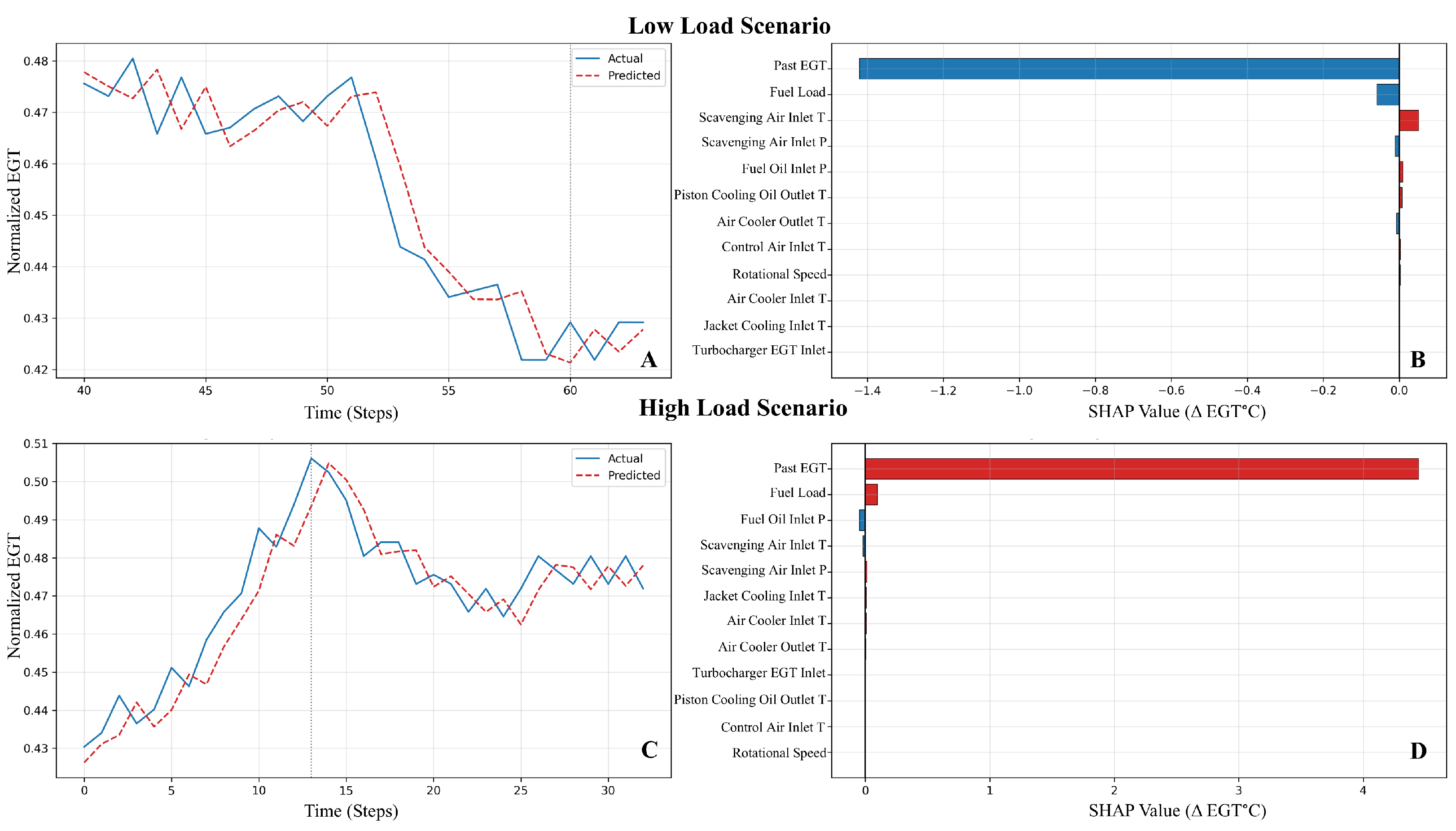
Figure 6 provides local explanations for two representative cases, one at low load and one at high load. In each row, the left panel shows the normalized EGT trajectory together with the BEACON prediction, and the vertical dotted line marks the time instant for which the SHAP values in the right panel are computed. For the low load window in Figure 6A,B, the measured EGT is below its typical level and the model predicts a modest decrease. The SHAP bars indicate that this drop is driven almost entirely by negative contributions from past EGT, around 1.4 ° C , with a smaller effect from fuel load, while the remaining sensors contribute very little. In contrast, for the high load window in Figure 6C,D, the engine approaches a local maximum in EGT and BEACON tracks the rise closely. The local explanation attributes more than + 4 ° C to an elevated past EGT, with fuel load again providing a smaller positive increment and the air path and cooling system variables playing only a minor role. These two examples show that at the level of individual predictions, BEACON bases its decisions on the same dominant drivers that appear in the global analysis, namely recent exhaust temperature history and engine loading, and that the sign of their contributions aligns with engine thermodynamics.
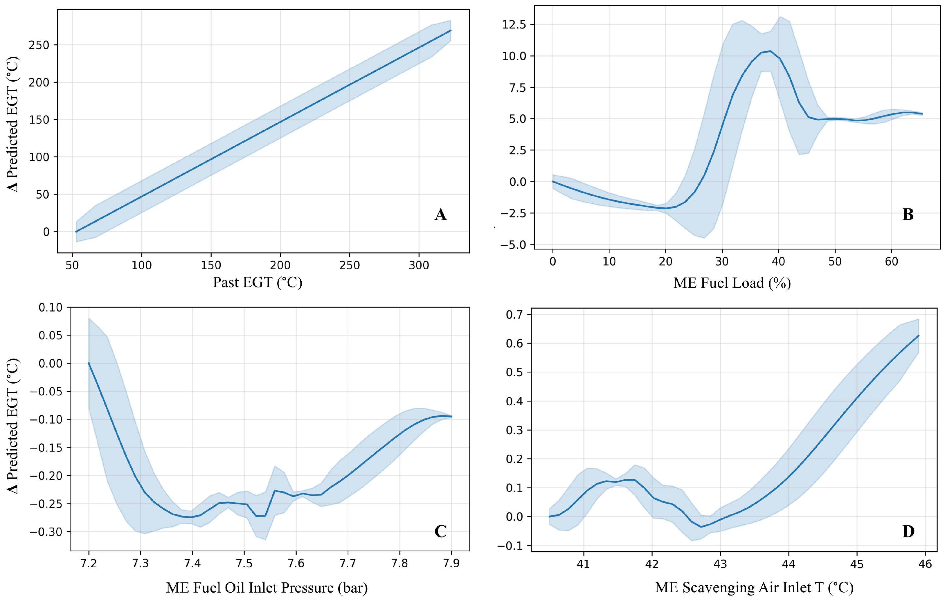
Figure 7 shows how BEACON responds to the four most influential inputs. Each curve reports the change in predicted Cylinder 1 EGT when a single feature is varied over its observed range while the remaining inputs are fixed at their median values. The shaded region reflects the spread of individual conditional expectation curves, and all quantities are expressed in physical units.
Specifically, in Figure 7A, the response to past EGT is close to linear and strictly increases across the full range from about 50 ° C to 320 ° C . The slope remains almost constant and the uncertainty band is narrow, which is consistent with strong temporal persistence of exhaust temperature and confirms that recent EGT is the dominant driver in the model. It should be mentioned that the lower tail of the past EGT distribution (around 50 °C) corresponds to engine shutdown or cooldown. These points are rare and lie outside the typical sea-going PdM regime. Figure 7B shows the response to ME fuel load, where for very-low-to-moderate loads up to roughly 25 to 30 % , the model predicts a mild reduction in EGT. As the load enters the typical sea-going range, the curve rises steeply, reaching a local maximum of a more than 10 ° C increase in predicted EGT around 35 to 40 % , and then flattens toward a plateau at higher loads. This wider band between 30 and 40 % reflects the limited amount of data in this region and suggests stronger interactions with other variables.
Furthermore, Figure 7C,D correspond to fuel oil inlet pressure and scavenging air inlet temperature. Both inputs have a much smaller marginal effect than the past EGT and fuel load variables, with changes in predicted EGT in the order of a few tenths of a degree of ° C . In detail, fuel oil inlet pressure exhibits a shallow bowl-shaped response, with a minimum around 7.3 to 7.4 bar and a gradual recovery toward the edges of the range, which indicates a secondary corrective role. Meanwhile, the response to scavenging air temperature shows a gentle dip near 42 to 43 ° C , followed by a monotone increase up to about 46 ° C . This pattern is compatible with a preferred intake temperature band, outside which small increases in exhaust temperature are expected. Overall, the curves support the results from the SHAP analysis that BEACON learns a hierarchy in which past EGT and fuel load explain most of the variation, while fuel system and air path variables provide finer adjustments that remain physically plausible.

5.2. Federated Learning Evaluation

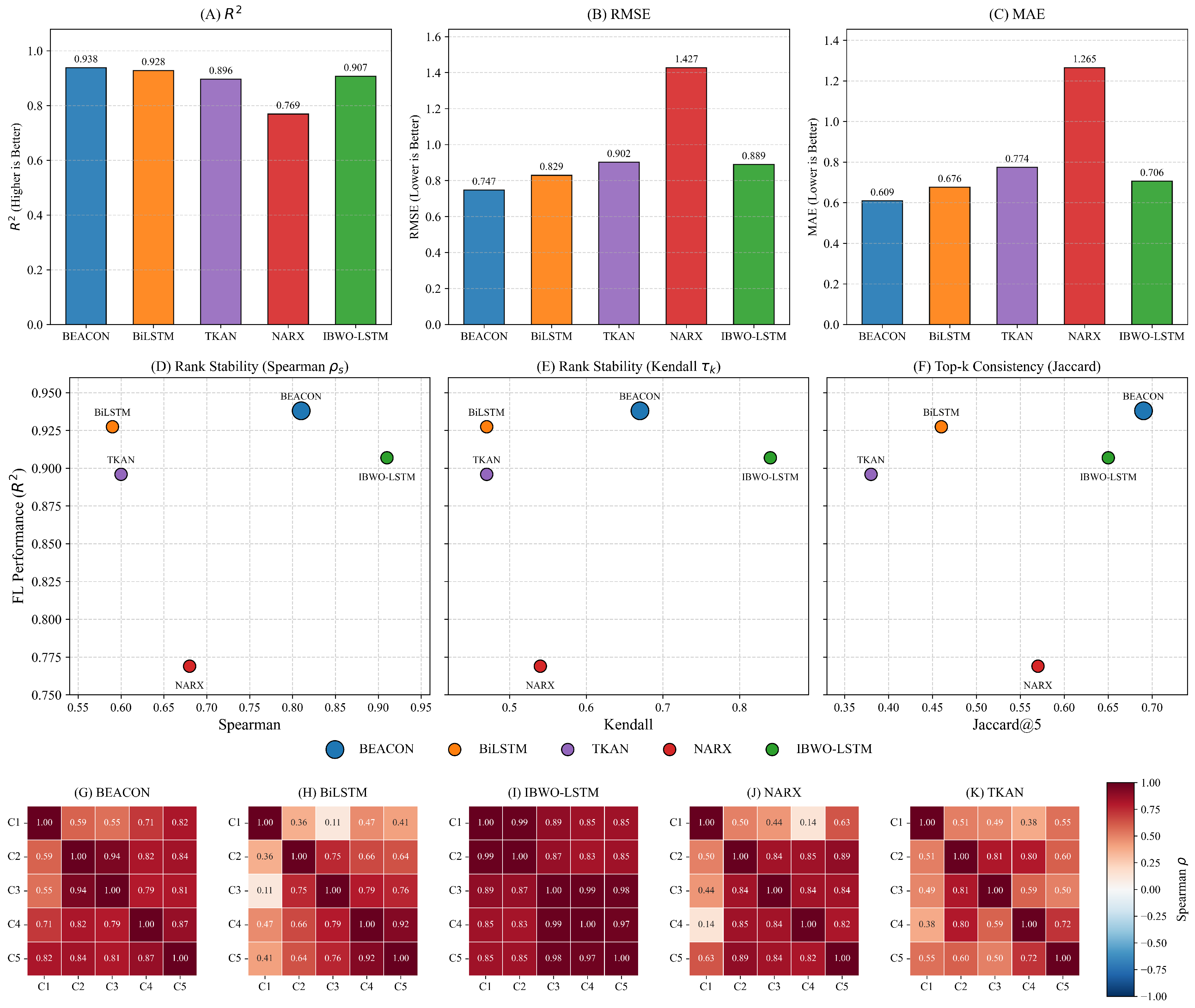
Figure 8 summarizes the federated experiments with five clients under Dirichlet partitioning with α being 1.0 . In Figure 8A–C, BEACON attains the highest federated R 2 ( 0.938 ) and the lowest RMSE and MAE ( 0.747 and 0.609 , respectively), improving RMSE and MAE by roughly 10% relative to the BiLSTM baseline. TKAN and IBWO-LSTM reach intermediate accuracy, while NARX shows clearly inferior performance, with its RMSE above 1.4 and MAE above 1.2 . These results indicate that the KAN head and attention pooling preserve predictive accuracy when moving from centralized to FL training.
Figure 8D–F link the federated R 2 to client-wise explanation stability. For BEACON, the mean Spearman and Kendall correlations of the client-level SHAP rankings are around 0.8 and 0.6 , and the Jaccard index on the top five features is close to 0.7 . BiLSTM and TKAN achieve similar or lower R 2 values but exhibit weaker agreement in both their rank and top feature sets. IBWO-LSTM shows high stability but with noticeably lower accuracy, while NARX is dominated on both axes. The client-wise heatmaps in Figure 8G–K further confirm this pattern, where BEACON maintains consistently high pair-wise correlations between clients, whereas BiLSTM, TKAN and NARX display several client pairs with much lower agreement. In practice, this suggests that BEACON offers a more favourable balance between federated accuracy and cross-client coherence of explanations.

5.3. Ablation Analysis

Table 3 quantifies the contribution of the main architectural choices in BEACON. The KAN-MLP variant, which removes the recurrent backbone and relies only on a KAN block with a shallow MLP head, shows poor performance. Its RMSE is around 3.31 and its MAE is close to 2.71 , more than four times higher than the recurrent variants, and its mean R 2 is negative with substantial variability. This indicates that a KAN head on its own cannot capture the temporal structure of the ME sensor streams and that an explicit sequence encoder is needed for heterogeneous client data.
Furthermore, replacing the dense output head of the BiLSTM-MLP baseline with a KAN head yields a consistent improvement. BiLSTM-KAN reduces the RMSE from 0.7584 to 0.7475 and lowers the MAE from 0.6743 to 0.6094 . The coefficient of determination increases from 0.9290 to 0.9353 , and the standard deviations for all three metrics are smaller than those of BiLSTM-MLP. This shows that the KAN block could provide more suitable mapping from latent temporal features to EGT than a purely dense MLP head.
The full BEACON architecture, which combines the BiLSTM encoder with attention pooling, the KAN block and the residual regression head, achieves the best overall trade-off. Compared with BiLSTM-MLP, the model’s RMSE decreases from 0.7584 to 0.7466 and its MAE decreases from 0.6743 to 0.6087 , while its R 2 increases to 0.9381 . Relative to BiLSTM-KAN, BEACON brings a small but consistent gain in accuracy and a further reduction in variance. These results suggest that the complete BEACON design leads to both higher accuracy and more stable training across federated runs.

6. Conclusions

In this work, we presented BEACON, a hybrid BiLSTM-Att-KAN-MLP architecture for cylinder EGT prediction on marine MEs, evaluated in both centralized and federated settings. In centralized training, BEACON consistently achieved the lowest error among the PdM baselines, with RMSE and MAE reductions relative to a strong BiLSTM encoder and an R 2 close to 0.95 . The ablation study showed that this gain is not due to the recurrent encoder alone. Replacing a dense MLP head with a KAN head improved RMSE for the same BiLSTM backbone, which indicates that the spline-based KAN layer is better suited than a fixed activation MLP to capture the nonlinear EGT response to changing ME operating conditions. A KAN-only variant without the recurrent backbone performed poorly, which underlines that temporal memory and KAN expressiveness are complementary rather than interchangeable. The explainability analysis further supports that BEACON learns a physically plausible hierarchy of drivers. SHAP summaries consistently placed past EGT and fuel load at the top of the ranking, with air path and cooling variables acting as smaller corrections. Local explanations in low and high load windows showed that individual predictions depend on the same variables, with signs and magnitudes that matched expected ME behaviour. Partial dependence curves reconstructed from the spline heads were smooth functions in physical units and agreed with known trends such as strong persistence in EGT and monotone increase with load in the sea-going range. Taken together, these results further support the view that BEACON achieves high accuracy while retaining a transparent mapping from inputs to EGT. However, it should be noted that the main value of BEACON is its accuracy–stability trade-off, and not raw error alone.
Under FL settings with Dirichlet partitioning, BEACON maintained competitive accuracy across five clients and converged reliably with the standard FedAvg strategy. A more important finding is the behaviour of the explanations. Baseline models that reached similar RMSE values showed marked divergence in their SHAP-based feature rankings across clients, with rank correlations sometimes dropping toward values near zero and Jaccard similarities below moderate levels. This is an indication of predictive multiplicity or the Rashomon effect, where different local models explain the same target in incompatible ways [56]. In contrast, BEACON preserved higher cross-client agreement in similarity scores, indicating that the combination between the attention and KAN head tend to filter out client-specific sampling variables and converge to a common, potentially physically meaningful explanation. For maintenance practices, this per-client stability could be considered as important as raw error, since ship-specific models are used to justify interventions and conflicting explanations across vessels can erode trust even when the global loss is low.
Concerning the limitations and future research directions of this work, there are several extensions to consider. All experiments were carried out on data from a single bulk carrier, with one ME cylinder as the prediction target, which limits the diversity of operating conditions, engine types and fuel configurations represented. The FL study used five clients and the standard FedAvg aggregation rule, which is known to degrade under non-IID client data [57,58]. In this study, FedAvg is adopted deliberately as a widely used baseline so that observed differences in accuracy and explanation stability can be attributed primarily to the model architectures rather than to specialized aggregation mechanisms. A systematic comparison with non-IID robust or personalized FL strategies, combined with an explicit treatment of communication constraints, privacy mechanisms and adversarial behaviour, is therefore regarded as a separate line of work.
Additionally, future studies should test whether the observed stability of explanations persists under stronger non-IID conditions, for example more skewed Dirichlet partitions (e.g., a { 0.1 , 0.3 , 0.5 , 1 , 10 } ), and under alternative FL strategies that address client drift or fairness objectives, using data from additional vessels and fleets with different engine, fuel types and operating profiles. Furthermore, the impact of secure aggregation, homomorphic encryption and differential privacy noise on both predictive accuracy and explanation stability also needs to be quantified. On the modelling side, it will be important to reduce the latency of the KAN block, for example through spline quantization or parameter sharing, and to validate BEACON on multi-cylinder and emission-oriented targets across multiple ME types. In the present study, attention pooling was adopted as a lightweight temporal aggregator that matches deployment constraints, and a systematic comparison with self-attention mechanisms or Transformer-based encoders is left for future work to avoid confounding architectural effects. Overall, the findings of this work suggest that BEACON is a practical step toward accurate and explanation-stable federated PdM for marine engines.

Author Contributions

Conceptualization, A.S.K.; methodology, A.S.K., G.L. and A.G.; software, A.S.K. and G.L.; validation, A.S.K.; data curation, N.T.; writing—original draft preparation, A.S.K.; writing—review and editing, A.S.K., A.G. and P.T.; supervision, P.T. All authors have read and agreed to the published version of the manuscript.

Funding

This research study received no external funding.

Data Availability Statement

The datasets presented in this article are not readily available due to commercial constraints. However, access to the datasets can be provided upon request from the corresponding author.

Acknowledgments

The authors would like to thank Laskaridis Shipping Co., Ltd., for data provision.

Conflicts of Interest

Author Nikolaos Tsoulakos is employed by Laskaridis Shipping Co., Ltd. The remaining authors declare that the research was conducted in the absence of any commercial or financial relationships that could be construed as a potential conflict of interest.

Abbreviations

The following abbreviations are used in this manuscript:
BiLSTMBidirectional long short-term memory network
EGTExhaust gas temperature
FedAvgFederated averaging
FLFederated learning
IBWO-LSTMLSTM tuned with Improved Binary Whale Optimization
J @ 5 Jaccard index on the top five ranked features
KNumber of B-spline basis functions per KAN map
KANKolmogorov Arnold network
LNumber of BiLSTM layers
MAEMean absolute error
MEMain engine
NNumber of samples in an evaluation set
NARXNonlinear autoregressive model with exogenous inputs
PdMPredictive maintenance
R 2 Coefficient of determination
RMSERoot mean square error
SHAPShapley Additive Explanations
TSequence length (time steps per input window)
TKANTemporal Kolmogorov Arnold network
XAIExplainable artificial intelligence
α Dirichlet concentration parameter for client partitioning
dNumber of input features
hHidden size per LSTM direction
μ y , σ y Mean and standard deviation of EGT in the training set
X t Multivariate input window at decision time t
y t + 1 Physical EGT target at time t + 1
ρ S Spearman rank correlation between SHAP rankings
τ k Kendall rank correlation between SHAP rankings

References

  1. Aslam, S.; Michaelides, M.P.; Herodotou, H. Internet of ships: A survey on architectures, emerging applications, and challenges. IEEE Internet Things J. 2020, 7, 9714–9727. [Google Scholar] [CrossRef]
  2. Kalafatelis, A.S.; Nomikos, N.; Giannopoulos, A.; Trakadas, P. A Survey on Predictive Maintenance in the Maritime Industry Using Machine and Federated Learning. TechRxiv 2024. [Google Scholar] [CrossRef]
  3. Maione, F.; Lino, P.; Maione, G.; Giannino, G. A machine learning framework for condition-based maintenance of marine diesel engines: A case study. Algorithms 2024, 17, 411. [Google Scholar] [CrossRef]
  4. International Maritime Organization (IMO). 2023 IMO Strategy on Reduction of GHG Emissions from Ships; IMO: London, UK, 2023. [Google Scholar]
  5. Hughes, E. FuelEU Maritime—Avoiding Unintended Consequences; European Community Shipowners’ Associations (ECSA): Brussels, Belgium, 2021. [Google Scholar]
  6. Flodén, J.; Zetterberg, L.; Christodoulou, A.; Parsmo, R.; Fridell, E.; Hansson, J.; Rootzén, J.; Woxenius, J. Shipping in the EU emissions trading system: Implications for mitigation, costs and modal split. Clim. Policy 2024, 24, 969–987. [Google Scholar] [CrossRef]
  7. Mrzljak, V.; Žarković, B.; Prpić-Oršić, J. Marine Slow Speed Two-Stroke Diesel Engine–Numerical Analysis of Efficiencies and Important Operating Parameters. Mach. Technol. Mater. 2017, 11, 481–484. [Google Scholar]
  8. Pavlenko, N.; Comer, B.; Zhou, Y.; Clark, N.; Rutherford, D. The Climate Implications of Using LNG as a Marine Fuel; Swedish Environmental Protection Agency: Stockholm, Sweden, 2020. [Google Scholar]
  9. Xin, M.; Gan, H.; Cong, Y.; Wang, H. Numerical simulation of methane slip from marine dual-fuel engine based on hydrogen-blended natural gas strategy. Fuel 2024, 358, 130132. [Google Scholar] [CrossRef]
  10. Meng, L.; Gan, H.; Liu, H.; Lu, D. Deep learning-based research on fault warning for marine dual fuel engines. Brodogr. Int. J. Nav. Archit. Ocean. Eng. Res. Dev. 2025, 76, 1–28. [Google Scholar] [CrossRef]
  11. Zhu, T.; Ran, Y.; Zhou, X.; Wen, Y. A survey of predictive maintenance: Systems, purposes and approaches. arXiv 2019, arXiv:1912.07383. [Google Scholar]
  12. Kalafatelis, A.S.; Nomikos, N.; Giannopoulos, A.; Alexandridis, G.; Karditsa, A.; Trakadas, P. Towards predictive maintenance in the maritime industry: A component-based overview. J. Mar. Sci. Eng. 2025, 13, 425. [Google Scholar] [CrossRef]
  13. Korczewski, Z. Exhaust gas temperature measurements in diagnostics of turbocharged marine internal combustion engines Part II dynamic measurements. Pol. Marit. Res. 2016, 23, 68–76. [Google Scholar] [CrossRef]
  14. Kumar, A.; Srivastava, A.; Goel, N.; McMaster, J. Exhaust gas temperature data prediction by autoregressive models. In Proceedings of the 2015 IEEE 28th Canadian Conference on Electrical and Computer Engineering (CCECE), Halifax, NS, Canada, 3–6 May 2015; pp. 976–981. [Google Scholar]
  15. Ji, Z.; Gan, H.; Liu, B. A deep learning-based fault warning model for exhaust temperature prediction and fault warning of marine diesel engine. J. Mar. Sci. Eng. 2023, 11, 1509. [Google Scholar] [CrossRef]
  16. Wang, B.; Wang, Z.; Yao, C.; Chen, J.; Lu, L.; Song, E. Multi-system condition monitoring of marine engines: A unified deep learning framework introducing physical prior knowledge. Int. J. Nav. Archit. Ocean Eng. 2025, 17, 100698. [Google Scholar] [CrossRef]
  17. Leifsson, L.Þ.; Sævarsdóttir, H.; Sigurðsson, S.Þ.; Vésteinsson, A. Grey-box modeling of an ocean vessel for operational optimization. Simul. Model. Pract. Theory 2008, 16, 923–932. [Google Scholar] [CrossRef]
  18. Park, S.; Noh, Y.; Kang, Y.J.; Sim, J.; Jang, M. An integrated grey-box model for accurate ship engine performance prediction under varying speed and environmental conditions. Int. J. Engine Res. 2024, 25, 1093–1110. [Google Scholar] [CrossRef]
  19. Zhang, Y.; Liu, P.; He, X.; Jiang, Y. A prediction method for exhaust gas temperature of marine diesel engine based on LSTM. In Proceedings of the 2020 IEEE 2nd International Conference on Civil Aviation Safety and Information Technology (ICCASIT), Weihai, China, 14–16 October 2020; pp. 49–52. [Google Scholar]
  20. Su, Y.; Gan, H.; Ji, Z. Research on multi-parameter fault early warning for marine diesel engine based on PCA-CNN-BiLSTM. J. Mar. Sci. Eng. 2024, 12, 965. [Google Scholar] [CrossRef]
  21. Barhrhouj, A.; Ananou, B.; Ouladsine, M. Exploring Explainable Machine Learning for Enhanced Ship Performance Monitoring. In Machine Learning, Optimization, and Data Science; Springer: Cham, Swizterland, 2024; pp. 1–13. [Google Scholar]
  22. Höhn, D.; Mumm, L.; Reitz, B.; Tsiroglou, C.; Hahn, A. Enabling Future Maritime Traffic Management: A Decentralized Architecture for Sharing Data in the Maritime Domain. J. Mar. Sci. Eng. 2025, 13, 732. [Google Scholar] [CrossRef]
  23. Kalafatelis, A.S.; Nikolakakis, V.; Tsoulakos, N.; Trakadas, P. Privacy-Preserving Hierarchical Federated Learning over Data Spaces. In Proceedings of the 13th IEEE International Conference on Big Data 2025 (BigData), Macau, China, 8–11 December 2025; pp. 6424–6433. [Google Scholar]
  24. Doulkeridis, C.; Santipantakis, G.M.; Koutroumanis, N.; Makridis, G.; Koukos, V.; Theodoropoulos, G.S.; Theodoridis, Y.; Kyriazis, D.; Kranas, P.; Burgos, D.; et al. Mobispaces: An architecture for energy-efficient data spaces for mobility data. In Proceedings of the 2023 IEEE International Conference on Big Data (BigData), Sorrento, Italy, 15–18 December 2023; pp. 1487–1494. [Google Scholar]
  25. McMahan, B.; Moore, E.; Ramage, D.; Hampson, S.; y Arcas, B.A. Communication-efficient learning of deep networks from decentralized data. In Proceedings of the 20th Artificial Intelligence and Statistics, Fort Lauderdale, FL, USA, 20–22 April 2017; pp. 1273–1282. [Google Scholar]
  26. Karimireddy, S.P.; Kale, S.; Mohri, M.; Reddi, S.; Stich, S.; Suresh, A.T. Scaffold: Stochastic controlled averaging for federated learning. In Proceedings of the 37th International Conference on Machine Learning PMLR, Virtual Event, 13–18 July 2020; pp. 5132–5143. [Google Scholar]
  27. Alvarez-Melis, D.; Jaakkola, T.S. On the robustness of interpretability methods. arXiv 2018, arXiv:1806.08049. [Google Scholar] [CrossRef]
  28. Cossu, A.; Spinnato, F.; Guidotti, R.; Bacciu, D. Drifting explanations in continual learning. Neurocomputing 2024, 597, 127960. [Google Scholar] [CrossRef]
  29. Bogdanova, A.; Imakura, A.; Sakurai, T. DC-SHAP method for consistent explainability in privacy-preserving distributed machine learning. Hum.-Centric Intell. Syst. 2023, 3, 197–210. [Google Scholar] [CrossRef]
  30. Hossain, M.A.; Saif, S.; Islam, M.S. A novel federated learning approach for IoT botnet intrusion detection using SHAP-based knowledge distillation. Complex Intell. Syst. 2025, 11, 422. [Google Scholar] [CrossRef]
  31. Liu, Z.; Wang, Y.; Vaidya, S.; Ruehle, F.; Halverson, J.; Soljačić, M.; Hou, T.Y.; Tegmark, M. Kan: Kolmogorov-arnold networks. arXiv 2024, arXiv:2404.19756. [Google Scholar]
  32. Raptodimos, Y.; Lazakis, I. Application of NARX neural network for predicting marine engine performance parameters. Ships Offshore Struct. 2020, 15, 443–452. [Google Scholar] [CrossRef]
  33. Sun, J.; Zeng, H.; Ye, K. Short-term exhaust gas temperature trend prediction of a marine diesel engine based on an improved slime mold algorithm-optimized bidirectional long short-term memory—Temporal pattern attention ensemble model. J. Mar. Sci. Eng. 2024, 12, 541. [Google Scholar] [CrossRef]
  34. Gao, B.; Xu, J.; Zhang, Z.; Liu, Y.; Chang, X. Marine diesel engine piston ring fault diagnosis based on LSTM and improved beluga whale optimization. Alex. Eng. J. 2024, 109, 213–228. [Google Scholar] [CrossRef]
  35. Dejanović, M.; Panić, S.; Kontrec, N.; Đošić, D.; Milojević, S. Neural Network-Based Optimization of Repair Rate Estimation in Performance-Based Logistics Systems. Information 2025, 16, 1031. [Google Scholar] [CrossRef]
  36. Vaca-Rubio, C.J.; Blanco, L.; Pereira, R.; Caus, M. Kolmogorov-arnold networks (kans) for time series analysis. arXiv 2024, arXiv:2405.08790. [Google Scholar] [CrossRef]
  37. Xu, K.; Chen, L.; Wang, S. Kolmogorov-arnold networks for time series: Bridging predictive power and interpretability. arXiv 2024, arXiv:2406.02496. [Google Scholar] [CrossRef]
  38. Genet, R.; Inzirillo, H. TKAN: Temporal Kolmogorov-Arnold Networks. arXiv 2025, arXiv:2405.07344. [Google Scholar] [CrossRef]
  39. Lipton, Z.C. The mythos of model interpretability: In machine learning, the concept of interpretability is both important and slippery. Queue 2018, 16, 31–57. [Google Scholar] [CrossRef]
  40. Doshi-Velez, F.; Kim, B. Towards a rigorous science of interpretable machine learning. arXiv 2017, arXiv:1702.08608. [Google Scholar] [CrossRef]
  41. Adebayo, J.; Gilmer, J.; Muelly, M.; Goodfellow, I.; Hardt, M.; Kim, B. Sanity checks for saliency maps. In Proceedings of the 32nd International Conference on Neural Information Processing Systems (NeurIPS), Montréal, QC, Canada, 3–8 December 2018. [Google Scholar]
  42. Kim, D.; Antariksa, G.; Handayani, M.P.; Lee, S.; Lee, J. Explainable anomaly detection framework for maritime main engine sensor data. Sensors 2021, 21, 5200. [Google Scholar] [CrossRef]
  43. Je-Gal, H.; Park, Y.S.; Park, S.H.; Kim, J.U.; Yang, J.H.; Kim, S.; Lee, H.S. Time-series explanatory fault prediction framework for marine main engine using explainable artificial intelligence. J. Mar. Sci. Eng. 2024, 12, 1296. [Google Scholar] [CrossRef]
  44. Visser, R.; Peters, T.M.; Scharlau, I.; Hammer, B. Trust, distrust, and appropriate reliance in (X) AI: A conceptual clarification of user trust and survey of its empirical evaluation. Cogn. Syst. Res. 2025, 91, 101357. [Google Scholar] [CrossRef]
  45. Papenmeier, A.; Englebienne, G.; Seifert, C. How model accuracy and explanation fidelity influence user trust. arXiv 2019, arXiv:1907.12652. [Google Scholar] [CrossRef]
  46. Kundu, R.K.; Hoque, K.A. Explainable predictive maintenance is not enough: Quantifying trust in remaining useful life estimation. Annu. Conf. PHM Soc. 2023, 15, 1–15. [Google Scholar] [CrossRef]
  47. Gao, Z.W.; Xiang, Y.; Lu, S.; Liu, Y. An optimized updating adaptive federated learning for pumping units collaborative diagnosis with label heterogeneity and communication redundancy. Eng. Appl. Artif. Intell. 2025, 152, 110724. [Google Scholar] [CrossRef]
  48. Zhuang, Y.; Li, Y.; Song, Y.; Qiu, M. Personalized federated learning for fault diagnosis with mixture of experts. Inf. Fusion 2025, 125, 103439. [Google Scholar] [CrossRef]
  49. Wang, G. Interpret federated learning with shapley values. arXiv 2019, arXiv:1905.04519. [Google Scholar] [CrossRef]
  50. Pirie, C.; Wiratunga, N.; Wijekoon, A.; Moreno-Garcia, C.F. AGREE: A feature attribution aggregation framework to address explainer disagreements with alignment metrics. In Proceedings of the CEUR Workshop Proceedings, Aberdeen, UK, 17 July 2023; Volume 3438. [Google Scholar]
  51. Kalafatelis, A.S.; Pitsiakou, A.; Nomikos, N.; Tsoulakos, N.; Syriopoulos, T.; Trakadas, P. FLUID: Dynamic Model-Agnostic Federated Learning with Pruning and Knowledge Distillation for Maritime Predictive Maintenance. J. Mar. Sci. Eng. 2025, 13, 1569. [Google Scholar] [CrossRef]
  52. Liu, B.; Gan, H.; Chen, D.; Shu, Z. Research on fault early warning of marine diesel engine based on CNN-BiGRU. J. Mar. Sci. Eng. 2022, 11, 56. [Google Scholar] [CrossRef]
  53. Cohen, J. Statistical Power Analysis for the Behavioral Sciences; Routledge: New York, NY, USA, 2013. [Google Scholar]
  54. Zhang, Y.; Zhang, Y. FedPDC: Federated Learning for Public Dataset Correction. arXiv 2023, arXiv:2302.12503. [Google Scholar]
  55. Lundberg, S.M.; Lee, S.I. A unified approach to interpreting model predictions. In Proceedings of the 31st International Conference on Neural Information Processing Systems (NeurIPS), Long Beach, CA, USA, 4–9 December 2017. [Google Scholar]
  56. Müller, S.; Toborek, V.; Beckh, K.; Jakobs, M.; Bauckhage, C.; Welke, P. An empirical evaluation of the Rashomon effect in explainable machine learning. In Machine Learning and Knowledge Discovery in Databases: Research Track; Springer: Cham, Switzerland, 2023; pp. 462–478. [Google Scholar]
  57. Li, X.; Huang, K.; Yang, W.; Wang, S.; Zhang, Z. On the convergence of fedavg on non-iid data. arXiv 2019, arXiv:1907.02189. [Google Scholar]
  58. Qu, L.; Zhou, Y.; Liang, P.P.; Xia, Y.; Wang, F.; Adeli, E.; Li, F.-F.; Rubin, D. Rethinking architecture design for tackling data heterogeneity in federated learning. In Proceedings of the IEEE/CVF Conference on Computer Vision and Pattern Recognition, New Orleans, LA, USA, 18–24 June 2022; pp. 10061–10071. [Google Scholar]
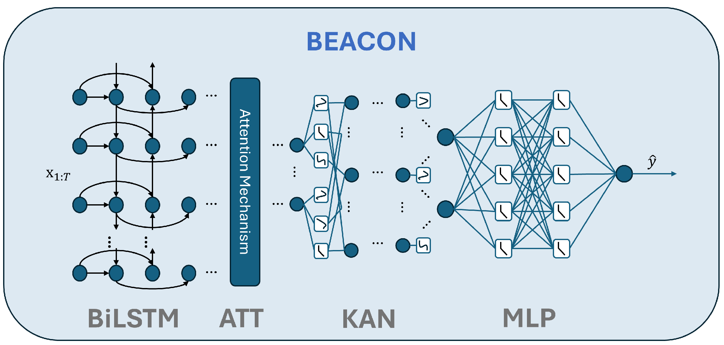
Figure 1. High-level overview of the BEACON architecture.
Jmse 14 00032 g001
Figure 2. Architectural comparison between a standard MLP and a KAN.
Jmse 14 00032 g002
Figure 3. FL configuration used in this study, where a central coordinator aggregates model updates from clients using FedAvg over a non-IID partition.
Jmse 14 00032 g003
Figure 4. Centralized validation performance of BEACON and baselines. The top panel shows scatter plots of the predicted versus measured Cylinder EGT on the validation set, with panels (AE) corresponding to BEACON, BiLSTM, TKAN, NARX and IBWO-LSTM, respectively. The dashed red line indicates perfect prediction and the solid green line is a least-squares fit. The bottom panel is a representative validation time series for Cylinder EGT showing the measured EGT (black line), BEACON prediction (blue line) and the associated confidence band.
Jmse 14 00032 g004
Figure 5. Global explanation of BEACON on the validation set. Panel (A) shows the SHAP summary plot, where each point corresponds to the contribution of one feature to the predicted Cylinder EGT for a single sample, expressed as Δ EGT ( ° C ). Panel (B) shows regime-wise mean absolute SHAP values, computed separately for low- and high-load scenarios.
Jmse 14 00032 g005
Figure 6. Local explanations for representative low load and high load windows. Panels (A,C) show the normalized Cylinder EGT and the corresponding BEACON prediction over the selected time windows. Panels (B,D) report the SHAP values at the marked prediction time, expressed as Δ EGT ( ° C ).
Jmse 14 00032 g006
Figure 7. One-dimensional response of BEACON for EGT prediction. Panels (AD) show partial dependence curves for past EGT, fuel load, fuel oil inlet pressure and scavenging air inlet temperature, respectively. The shaded bands indicate the dispersion of individual conditional expectation curves around the mean response.
Jmse 14 00032 g007
Figure 8. Federated performance and explanation stability across architectures. (AC) Federated learning regression metrics for the five models, i.e., R 2 , RMSE and MAE, respectively. (DF) Trade-off between federated performance and explanation stability, i.e., FL R 2 compared to mean Spearman, Kendall and Jaccard similarity of SHAP feature rankings across clients. (GK) Client-per-client Spearman correlation matrices of SHAP rankings for each model.
Jmse 14 00032 g008
Table 1. Engine-related features retained after correlation screening.
Feature (Symbol)UnitMain Role
Engine speedrpmIndicates ME operating point and load level
Fuel load%Proxy for thermal loading and combustion demand
Scavenge air pressurebarReflects charge air density and gas clearing
Piston cooling oil outlet ° C Local piston and liner thermal state
Air cooler air inlet ° C Charge air temperature before the cooler
Air cooler air outlet ° C Effectiveness of the charge air cooler
Jacket water inlet ° C Baseline cylinder cooling level
Fuel oil inlet pressurebarHealth of the fuel supply and filtration train
Scavenge air inlet ° C Intake air temperature to the scavenging blower
Turbocharger inlet EGT ° C Turbine inlet thermal loading and backpressure
Control air pressurebarAvailability of pneumatic pressure for engine control
Past Cylinder 1 EGT ° C Autoregressive driver for the target exhaust temperature
Table 2. Centralized performance and computational profile of PdM models.
ModelRMSEMAER2Parameters (M)
BiLSTM0.7052 ± 0.00760.5654 ± 0.00700.9473 ± 0.00113.9315
IBWO-LSTM1.0352 ± 0.19480.8342 ± 0.16500.8826 ± 0.04670.2832
NARX1.3791 ± 0.23351.0621 ± 0.16870.7957 ± 0.06970.0380
TKAN0.7839 ± 0.17030.6152 ± 0.12250.9327 ± 0.03130.3530
BEACON0.5905 ± 0.00510.4713 ± 0.00420.9496 ± 0.00097.9253
Table 3. Ablation study of BEACON components in the FL setup.
ModelRMSEMAER2
BiLSTM-MLP 0.7584 ± 0.0124 0.6743 ± 0.0148 0.9290 ± 0.0026
BiLSTM-KAN 0.7475 ± 0.0020 0.6094 ± 0.0018 0.9353 ± 0.0004
KAN-MLP 3.3083 ± 0.3659 2.7058 ± 0.3426 0.3238 ± 0.2995
BEACON 0.7466 ± 0.0006 0.6087 ± 0.0012 0.9381 ± 0.0002
Disclaimer/Publisher’s Note: The statements, opinions and data contained in all publications are solely those of the individual author(s) and contributor(s) and not of MDPI and/or the editor(s). MDPI and/or the editor(s) disclaim responsibility for any injury to people or property resulting from any ideas, methods, instructions or products referred to in the content.