A Study on the Evolution Law of the Early Nonlinear Plastic Shock Response of a Ship Subjected to Underwater Explosions

Abstract

Early-stage dynamic responses of naval structures under underwater explosion shock loads exhibit high-frequency, intense amplitude fluctuations and short durations, serving as critical factors for the development of plastic deformation and other damage characteristics. These structural dynamics demonstrate prominent nonlinear and non-stationary features. This study focuses on the nonlinear evolutionary patterns of early-stage plastic shock responses in underwater explosion-impacted ship structures. Utilizing phase space reconstruction, unimodal mapping, and symbolic dynamics theory, we analyze the nonlinear and non-stationary characteristics along with their evolutionary patterns in experimental data. First, scaled model experiments under varying shock factors were conducted based on a stiffened cylindrical shell prototype, investigating the spatiotemporal evolution of nonlinear and non-stationary dynamic responses under different shock loads while characterizing their uncertainty features. Second, model tests were performed on deck-type cabin structures and plate frameworks derived from a naval vessel’s deck prototype, further analyzing the evolutionary patterns of early-stage plastic dynamic responses and verifying the method’s effectiveness and universality. Research findings indicate that (1) early-stage plastic shock responses of ships under underwater explosions exhibit multiple dynamical behaviors including chaotic motion, periodic motion, and quasi-periodic motion, and (2) during the initial plastic phase, orbital parameters approximate 0.8, providing guidance for test condition setup and initial parameter selection in underwater explosion experiments on naval structures.

1. Introduction

The plastic deformation process of ship structures subjected to underwater explosion shock loading is closely correlated with multiple factors including incident loading characteristics, system initial conditions, structural boundary constraints, and geometric configurations. The dynamic behavior of ship structures under such extreme loading conditions exhibits prominent nonlinear and non-stationary characteristics [1,2,3]. Current research methodologies for analyzing the coupled dynamic responses of hull structures and systems under underwater explosion primarily employ simplified analytical approaches such as amplitude comparison, time-domain comparison, and frequency-domain comparison. However, these conventional methods fail to adequately capture the intrinsic nonlinear features inherent in the structural dynamic responses induced by underwater explosion shock loading. Consequently, conducting in-depth nonlinear characteristic analysis of the coupled nonlinear–non-stationary dynamic responses represents a research direction with significant engineering application value for enhancing structural survivability under underwater explosion scenarios [4,5].

The shock wave generated by an underwater explosion propagates through the ship’s space grillage structure at different phase velocities. During this propagation process, the wave encounters the boundary of the grillage structure, where it reflects and transmits. This waveform conversion results in the formation of a standing wave, which causes structural vibration. The mathematical model of vibration shock response is a multi-variable infinite-order self-consistent equation. After Taylor expansion, the equation contains infinite-order derivatives, which transforms the dynamic system from a finite-dimensional to an infinite-dimensional entity. The solution of the equation is diverse and uncertain, resulting in the nonlinearity and bifurcation of the shock response. Its dynamic behavior is an extremely complex nonlinear motion process.

The current state of the art in dynamic response analysis of underwater explosion ship structures can be broadly divided into two categories: (1) structural response research based on shock wave load characteristics such as shock wave pressure peak, pulse width and impulse [6,7,8,9], and (2) time-frequency conversion methods such as wavelet analysis, modal decomposition and energy distribution, which are used to analyze the structural response time series signals [10,11,12,13]. (3) Based on theoretical analysis, numerical simulation, and model testing, the bifurcation and catastrophe phenomena of structural response are studied [3,4,5,14]. The aforementioned method primarily examines the structural damage mode and the evolution of the late response. However, there are some limitations in the analysis of the uncertainty characteristics of the early dynamic response to impact. The results of the early plastic dynamic response analysis are still insufficient, and research on the nonlinear evolution law is even less so.

The early nonlinear dynamic behavior of an underwater explosion ship is complex, and the impact response is difficult to describe using a mathematical model. The general time series is mainly studied in the time domain or transform domain. In chaotic time series processing, the calculation of chaotic invariants and the establishment and prediction of chaotic models are carried out in phase space. Therefore, phase space reconstruction is used to process chaotic time series [15,16,17]. The coordinate delay method is employed to construct an m-dimensional phase space vector from the different time delays of the one-dimensional time series, as depicted in Formula (1), which portrays the nonlinear evolution process of the early shock response.

$$x\left(i\right)=\left\{x\left(i\right),x\left(i+\tau \right),\cdots ,x\left(i+\left(m-1\right)\tau \right)\right\}$$

(1)

The above equation is used to characterize the early impact response motion, which is represented by the x(i) numerical orbit. This is achieved by utilizing the orbit sequence in the phase space. In order to theoretically analyze the motion process of the system, it is necessary to solve the high-order equation and sort the data points x_i, as shown in Equation (2). However, solving the higher-order equation is a challenging task. Symbolic dynamics employs a straightforward symbolic language, RL, to construct a symbolic sequence that describes the evolution of nonlinear dynamic behavior. This approach is discussed in detail in references [18,19,20].

$$x_{i+1}=f\left(x_i\right)=f^2\left(x_{i-1}\right)=\cdots =f^{i+1}\left(x_0\right)$$

(2)

A significant body of experimental data [4,21,22] on the shock response of underwater explosion ship structures indicates that the dynamic response of such structures can be divided into two distinct phases: the transient early shock response and the late shock response. The transient early impact response is characterized by a number of unique attributes, including a high peak value, a high frequency, a short duration and a severe change. This phase represents an important stage in the plastic deformation and even structural damage of ship structures. Consequently, in this paper, the evolution of the early nonlinear plastic impact response on ship structures subjected to impact loads is studied by means of the phase space reconstruction method and symbolic dynamics.

2. Model Test

2.1. Construction of the Experimental Platform

Given the dimensions of the explosion pool and the analogous conversion relationship between the prototype and the model of a stiffened cylindrical shell structure, provided that the prototype and the model exhibit a single value of similarity, a 1:8 ship cabin model was designed under the guidance of the newly derived impact factor C₃ [23]. The length of the single-layer shell stiffened cylindrical shell model is 2.46 m, the diameter is 1.60 m, the ring rib spacing is 0.19 m, and the ring rib height is 62.8 mm. In order to mitigate the influence of the boundaries, one rib is extended at both ends to serve as a ballast tank. The total length of the model is 2.46 m, as illustrated in Figure 1.

$$C_3={\displaystyle \frac{\sqrt{W}}{R^{\raisebox{1ex}{$3$}\!\left/ \!\raisebox{-1ex}{$2$}\right.}}}$$

(3)

Figure 1. Cylindrical shell model.

In order to provide additional buoyancy for the cylindrical shell model to maintain balance during the test, and also to prevent the cabin model from sinking into the water due to damage, an impact-resistant tooling buoy structure was designed. The diameter of a single pontoon is 2 m, and the length is 4 m. The two pontoons are connected by a truss and plate frame structure to form an impact-resistant tooling structure. In the event of an underwater explosion, the movement of the cabin model is constrained, the impact of waves on the experimental results is mitigated, and the apparatus is conducive to water operation and installation, as illustrated in Figure 2.

Figure 2. Anti-impact buoy structure.

The anti-impact buoy is connected to the cylindrical shell model via a steel wire rope. The test explosive is then positioned on the plate frame structure within the anti-impact tooling structure via the spreader and wire rope. Four counterweight blocks are positioned beneath the cylindrical shell model. The cylindrical shell model is hoisted into the water by crane and then sunk into the water independently under the action of negative buoyancy, with a force of 4880.4 N. The cylindrical shell model test is then carried out, as shown in Figure 3.

Figure 3. Cylindrical shell model test system.

The model is subjected to a series of tests under varying operational conditions within the explosion pool. The specific operational conditions are presented in Table 1 [24,25].

Table 1. The specific working condition parameter table of the model cabin experiment.

Working Condition	Detonation Source Scale Ratio	Test Water Depth	Charge Quality (TNT)	Charge Density	Detonation Velocity	Impact Factor
1	1:8	13.47 m	7.4 kg	1630 kg/m3	6900	0.28
2	1:8	13.47 m	7.4 kg	1630 kg/m3	6900	0.35
3	1:8	13.47 m	7.4 kg	1630 kg/m3	6900	0.70

2.2. Acquisition of Test Data

In advance of the experiment, a numerical method is employed to simulate the response of the cabin under test conditions, analyze the response characteristics, and identify potential weaknesses in the local strength of the structure. Given the operational constraints of installing measuring instruments such as strain gauges, the strain measuring points are selected to assess the local strength. Finally, the strain measuring points are positioned on the pressure shell and ring ribs of the ship cabin. Specifically, 15 strain measuring points are arranged on the plate and shell of the pressure shell of the cabin section, and 5 measuring points are arranged on the internal profile. Measuring points 1 and 2 are in the three directions of X, Y, and Z, and measuring points 3 are X and Y two-way measuring points. The remaining are X-direction measuring points. The strain response is measured by the electric measurement method, and the strain test data is collected. The bonding position of the strain gauge is illustrated in Figure 4, and the spatial arrangement of the strain measuring points is depicted in Figure 5.

Figure 4. Local schematic diagram of strain gauge adhesion of the test model.

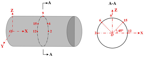
Figure 5. Schematic diagram of the strain test space layout.

3. Characteristics of Early Plastic Impact Response Signal

A cylindrical shell model was utilized to investigate the effects of various impact factors on an underwater explosion ship. When the new impact factor is set to 0.28, measuring point 6 exhibits plastic deformation. In the event that the new impact factor is 0.35, the following measuring points exhibit plastic deformation: 4, 5, 6, and 7. In the event that the new impact factor is 0.70, the aforementioned measuring points (4, 5, 6, 7, 13, 14, and 15) exhibit plastic deformation, as evidenced by the early plastic impact response signals depicted in Figure 6.

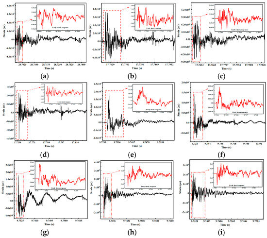
Figure 6. Early plastic shock response signal. (a) Measuring point 6 signal in working condition 1. (b) Measuring point 5 signal in working condition 2. (c) Measuring point 6 signal in working condition 2. (d) Measuring point 7 signal in working condition 2. (e) Measuring point 5 signal in working condition 3. (f) Measuring point 6 signal in working condition 3. (g) Measuring point 13 signal in working condition 3. (h) Measuring point 14 signal in working condition 3. (i) Measuring point 15 signal in working condition 3.

In the context of varying impact factors, the early dynamic response of the measuring points exhibiting plastic deformation in the underwater explosion model test evinces the characteristics of high frequency, high amplitude, and dramatic change, as well as the strong randomness of the time point of plastic occurrence. When the transient impact exceeds a certain critical value, the structure produces plastic deformation, which leads to the baseline drift of the impact response signal and the impact response becoming more disorganized. The uncertainty characteristics of the system dynamic behavior are more significant. The traditional analysis method struggles to characterize the evolution law of early plastic dynamic response. Therefore, this paper will use the phase space reconstruction method and symbolic dynamics to study the evolution law of early nonlinear plastic impact response.

4. Analysis of Early Nonlinear Plastic Impact Response

Although the early nonlinear dynamic behavior of a ship experiencing an underwater explosion is complex, and the mathematical model of plastic shock response is difficult to characterize; the general time series is mainly studied in the time domain or transform domain. In chaotic time series processing, whether it is the calculation of chaotic invariants, the establishment and prediction of chaotic models, or other related operations, they are carried out in phase space. This makes the performance of dynamic systems in phase space more intuitive and simple. Therefore, phase space reconstruction is employed to process chaotic time series [15,16,17]. Through the coordinate delay method, an m-dimensional phase space vector is constructed by different time delays of one-dimensional time series, as illustrated in Equation (1). The initial characteristics of the plastic impact response are transformed into phase space for analysis, and the initial nonlinear plastic impact response is studied.

In the model test of a stiffened cylindrical shell structure, the one-dimensional time series of strain changing with time at different measuring points are collected by strain gauge. According to the self-similarity of complex dynamic systems, that is, the time series of a single variable implies the motion law of the whole system, the appropriate delay τ is selected with the help of the phase space reconstruction method, and the strain time series is constructed into an m-dimensional phase space. The trajectory distribution or attractor in the reconstructed phase space is employed to elucidate the motion characteristics of the entire nonlinear dynamic system.

4.1. Time Series Reconstruction

In this paper, the dimension m and delay τ of the reconstructed phase space are determined according to the one-dimensional time series of strain. Compared with other fractal dimension methods, the correlation dimension can map high-dimensional data to a low-dimensional space to characterize the data structure and the characteristics of the data itself [20]. Therefore, the correlation dimension d₂ is used to determine the dimension m of the strain one-dimensional time series.

$$d_2=\underset{\epsilon \to 0}{\lim }\gamma =\underset{\epsilon \to 0}{\lim }{\displaystyle \frac{\ln C(\epsilon )}{\ln \epsilon }}$$

(4)

The dimension correlation quantity γ, is defined as the degree of data correlation in the phase space, C(ε), where ε represents the radius of the given ultra-small ball in the phase space.

$$C(\epsilon )=\underset{N\to \infty }{\lim }{\displaystyle \frac{1}{N(N-1)}}{\displaystyle \sum _{i\ne j}\theta (\epsilon -\left|x_i-x_j\right|)}$$

(5)

In the formula, N represents the number of data points in the phase space, while θ denotes the step function. For a specific range of ε, the relationship is shown in Equation (6).

$$C(\epsilon )=K{\epsilon }^{\gamma }$$

(6)

In the formula, K represents the proportional coefficient. The early plastic impact response signal exhibits high frequency, fast change, noise signal, and strong randomness. The dimension of the strain time series should be taken at the stable slope of the dimension slope, and the dimension of the dynamic system is 2, as illustrated in Figure 7.

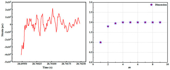
Figure 7. Dimension of early plastic impact response signal.

In the reconstructed phase space, if the delay τ is too small, then x(t + iτ) is approximately equal to x[t + (i + 1)τ], which results in an approximately diagonal trajectory, which is unable to reflect the motion characteristics of the system. If the delay τ is excessively large, then x(t + iτ) is entirely independent of x[t + (i + 1)τ], which is incompatible with the chaotic dynamics of nonlinear dynamic systems. Consequently, this paper employs the autocorrelation function [26] C(τ) to determine the optimal delay τ in the reconstructed phase space, as illustrated in Figure 8.

$$C(\tau )=\underset{T\to \infty }{\lim }{\displaystyle \frac{1}{T}}{\displaystyle {\int }_{-T/2}^{T/2}x(t)x(t+\tau )}dt$$

(7)

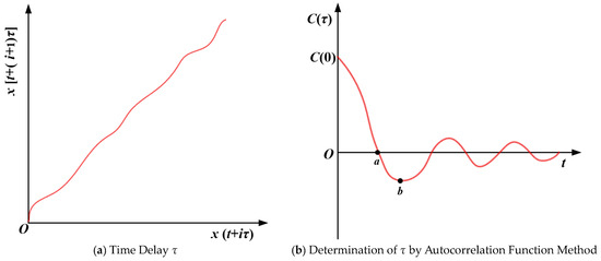
Figure 8. Calculation of optimal delay τ in phase space reconstruction.

In the case where C(τ) decreases with the increase in τ, the smaller the C(τ), the more independent the x(t + iτ) and x[t + (i + 1)τ] are. The delay τ is determined by the degree of dispersion of the early impact signal data itself. In general, C(τ) is reduced from C(0) to the first minimum, or C(τ) takes zero for the first time, as a measure of the regularity of the system. At this time, τ₀ is the correlation time, and x(t + iτ₀) and x[t + (i + 1)τ₀] are used to describe the motion process of the whole system.

4.2. Time Series Fitting Method

In the event that the newly calculated impact factor C₃ is 0.35 and the test water depth is 13.47 m, the embedding dimension of the six-axis (x-direction) strain time series of the ship cabin model test point is 2, and the delay amount is 15. The phase space reconstruction is employed to obtain the data trajectories x₁, x₂, x₃, x₄, x₅, x₆ and x₇ of the strain time series within the time interval Δt. This is accomplished within the scale-free range of the self-similarity of the test signal, as illustrated in Figure 9.

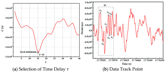
Figure 9. Time series phase space reconstruction.

The evolution process of the dynamic system during this time period is characterized by discrete mapping, as demonstrated by the difference shown in Equation (8).

$$x_{i+1}=F\left(u,x_i\right)$$

(8)

x_i is normalized, as demonstrated in Equation (9), and the iterative law of x_i is defined by discrete mapping.

$$y_i={\displaystyle \frac{x_i}{x_{\max }}}$$

(9)

The data point y_i, as shown in Table 2, is analyzed to determine its self-iteration law. It is found that y_i satisfies the logistic parabolic mapping [18,19,27], and it is fitted by Equation (9), as shown in Figure 10. The parameter u is standard.

$$y_{i+1}=F\left(u, y_i\right)=1-{u{y}_i}^2$$

(10)

Table 2. Normalized data.

yi	0	1	−0.58411	0.20004	0.866713	−0.25565	0.830283
yi+1	1	−0.58411	0.20004	0.866713	−0.25565	0.830283	−0.21538

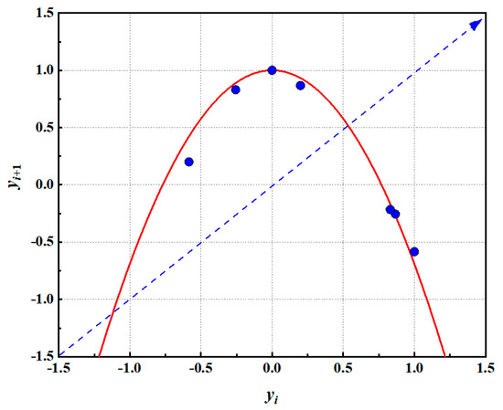
Figure 10. Fitting of the parabola.

The new impact factor C₃ is 0.28, and the strain time series of the axial strain of measuring point 6 is analyzed. The strain signal characteristic point xi of the axial strain signal of working condition 1–measuring point 6 in the scale-free range Δt period is selected through the phase space reconstruction method. x_i is normalized and discretely mapped to verify the correctness of the above analysis of the early nonlinear plastic impact response, as shown in Figure 11.

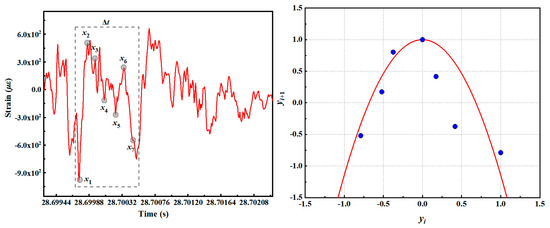
Figure 11. Discrete evolution of axial strain signal at measuring point 6 of condition 1.

When the new impact factor C₃ is 0.70, the strain time series of measuring points 13, 14, 15, and 6 are analyzed. The phase space reconstruction method is employed to identify the strain signal feature point xi of different signals within the scale-free range Δt period. x_i is then normalized and discretely mapped, as illustrated in Figure 12.

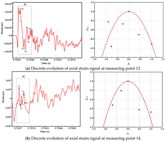
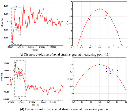
Figure 12. Discrete evolution of strain signals at axial measuring points of condition 3.

In the scale-free range Δt of the response signal, the discrete evolution of a large number of impact response signals shows that the early plastic impact response signals under different working conditions satisfy the parabolic mapping, and the time period is extended to Δt′. At this time, the early plastic impact response signal does not satisfy the parabolic mapping, taking the axial strain data of measuring point 6 of working condition 2 as an example, as shown in Figure 13.

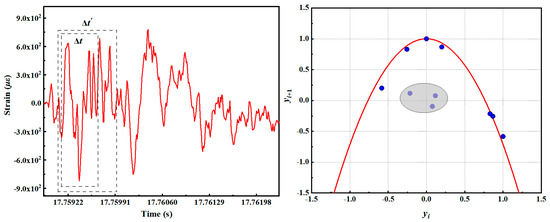
Figure 13. Schematic diagram of parabolic mapping orbit.

In conclusion, the impact response signal satisfies the parabolic mapping in the scale-free range Δt time of the response signal, while the impact response signal does not satisfy the parabolic mapping in the Δt′ time. Therefore, the early plastic impact response signal is divided into pieces, and the nonlinear characteristics of each plastic impact response signal are analyzed separately. A significant number of experimental data analysis results indicate that the scale-free range Δt time of different response signals is distinct, with the characteristic length being contingent upon the pulse width of the impact load, which is approximately 10 to 20 times the pulse width. The control parameter u of the parabolic map serves as a pivotal index for characterizing the nonlinear behavior of the early system. Variations in parameters result in disparate nonlinear dynamic behaviors [18,19,27]. As the parameter u is varied, the dynamic system undergoes period-doubling bifurcation and tangent bifurcation. The system transitions from stable periodic motion to quasi-periodic motion and then to chaotic motion. Each motion state appears alternately in the dynamic system. The sensitivity of the system to the initial value is enhanced, and the system exhibits more complex nonlinear characteristics. Consequently, the evolution law of the early plastic impact response can be described by analyzing the variation characteristics of the control parameter u in the process of the early plastic impact response. The branch diagram of parabolic mapping is shown in Figure 14.

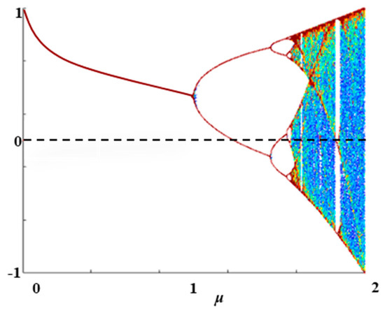
Figure 14. Unimodal mapping bifurcation diagram.

5. Evolution Law of Early Plastic Impact Response

Once the initial impact response signal has been mapped to the phase space, the system motion trajectory can be characterized by numerical trajectories such as x₁, x₂, x₃, x₄, x₅, x₆, and x₇. In order to analyze the motion process of the system, it is necessary to solve the high-order equation, as shown in Equation (1), and to sort the data points xi. Solving the high-order equation is a challenging task. If the exact value of each xi is not considered, only the range is considered. The initial point x₀ is taken as the boundary, the left point is counted as L, and the right point is counted as R. Each point position corresponds to a symbol s_i, and the definition of s_i is shown in Equation (11).

$$s_i=\left\{\begin{array}{c}L\begin{array}{cc}& x_i<x_0\end{array}\\ x_0\begin{array}{cc}& x_i=x_0\end{array}\\ R\begin{array}{cc}& x_i>x_0\end{array}\end{array}\right.$$

(11)

When the initial condition of the system is x₀, the evolution process can be expressed as the symbol sequence x₀ = s₀ s₁ s₂… s_n… In each iteration, the initial value changes from x₀ to x₁, and the symbol sequence becomes x₁ = s₁ s₂ s₃… s_n… Consequently, based on the scale-free range with self-similarity of the signal, the early plastic impact response signal is segmented, and the single-peak mapping function corresponding to each impact response signal is topologically conjugated to the symbolic dynamics. The parabolic mapping function and symbol sequence corresponding to each impact response signal are analyzed, and the evolution law of the early plastic impact response of the nonlinear dynamic system is studied by analyzing the data track in phase space, see Figure 15.

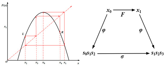
Figure 15. Topological conjugation.

The new impact factor C₃ is 0.35. The early plastic strain in the axial direction of measuring point 6 is divided into blocks for analysis. Each block has been reconstructed in phase space to fit the parameter u of the periodic orbit, and the nonlinear evolution process of the early plastic impact response has been characterized by the symbolic sequence. Concurrently, the theoretical parameter u_k is solved by the word lifting method in symbolic dynamics [9] to verify the accuracy of the fitting parameter u. The fitting of periodic orbits in different time periods is illustrated in Figure 16.

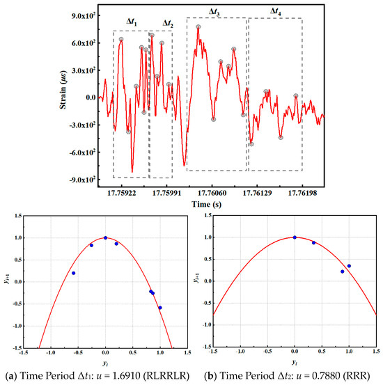
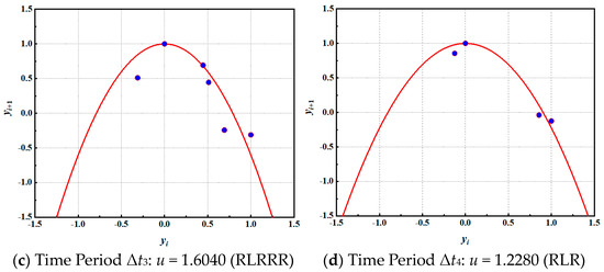
Figure 16. Periodic orbit fitting in different time periods of condition 2.

During time period Δt₁, the symbol sequence of the periodic orbit of the early plastic shock response is f₁ = RLRRLR. The equation obtained by the character lifting method is presented in Formula (12).

$$f\left(0\right)=R\circ L\circ R\circ R\circ L\circ R\left(0\right)$$

(12)

The two inverse functions are illustrated in Formula (13).

$$\begin{array}{l}R\left(y\right)=f_R^{-1}\left(y\right)=\sqrt{u^{-1}\left(1-y\right)}\\ L\left(y\right)=f_L^{-1}\left(y\right)=-\sqrt{u^{-1}\left(1-y\right)}\end{array}$$

(13)

Substituting Formula (13) into Formula (12), Formula (14) is obtained.

$$1=\sqrt{u^{-1}\left(1+\sqrt{u^{-1}\left(1-\sqrt{u^{-1}\left(1-\sqrt{u^{-1}\left(1+\sqrt{u^{-1}\left(1-\sqrt{u^{-1}}\right)}\right)}\right)}\right)}\right)}$$

(14)

Multiplied by u, Formula (15) is obtained.

$$u_{n+1}=\sqrt{u_n+\sqrt{u_n-\sqrt{u_n-\sqrt{u_n+\sqrt{u_n-\sqrt{u_n}}}}}}$$

(15)

The initial value of 0.5 is selected for the iterative solution, and the value of u_k is found to be 1.6741. The orbital parameter u, obtained by phase space reconstruction, is 1.6910.

At the time of Δt₂, the symbol sequence of the periodic orbit of the early plastic impact response is f₂ = RRR, with u_k = 0.8893 obtained by the word lifting method, and the fitted orbit parameter u is 0.7880. At the time of Δt₃, the symbol sequence of the periodic orbit of the early plastic impact response is f₃ = RLRRR, and u_k = 1.4760 is obtained. The fitted orbit parameter u is 1.6040. At the time of Δt₄, the symbol sequence of the periodic orbit of the early plastic impact response is f₄ = RLR, and u_k = 1.3151 is obtained. The fitted orbit parameter u is 1.2280. The accuracy of using different periodic orbit parameters to characterize the evolution process of the early plastic impact response is verified by fitting the periodic orbit parameters by the phase space reconstruction method. Consequently, under the condition that the new impact factor C₃ is 0.35, the evolution of the early plastic impact response in the axial direction of measuring point 6 is illustrated in Figure 17.

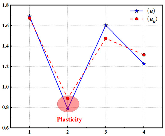
Figure 17. Evolution of early plastic impact response of condition 2.

The new impact factor C₃ is 0.28. The time series of the early plastic strain in the axial direction of measuring point 6 is divided into blocks. Figure 18 illustrates the parameter u of the fitting periodic orbit, as determined using the aforementioned phase space reconstruction method.

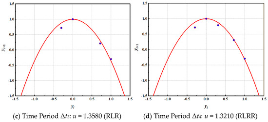
Figure 18. Periodic orbit fitting in different time periods of condition 1.

During the time period Δt₁, the symbol sequence of the periodic orbit of the early plastic impact response is f₁ = RLLRRL, with u_k = 1.9271 obtained by the word lifting method, and the fitted orbit parameter u is 1.9680. At the time of Δt₂, the symbol sequence of the periodic orbit of the early plastic impact response is f₂ = RRR, and u_k = 0.8893 is obtained. The fitted orbit parameter u is 0.7810. In the Δt₃ time, the symbol sequence of the periodic orbit of the early plastic impact response is f₃ = RLR, and the u_k = 1.3151 is obtained. The fitted orbit parameter u is 1.3580. In the Δt₄ time, the symbol sequence of the periodic orbit of the early plastic impact response is f₄ = RLRR, and the u_k = 1.6254 is obtained. The fitted orbit parameter u is 1.3210. The accuracy of using different periodic orbit parameters to characterize the evolution of the early plastic impact response is verified by fitting the periodic orbit parameters by the phase space reconstruction method. Therefore, the new impact factor C₃ is 0.28, and the early plastic impact response evolution of the measuring point 6 axis is shown in Figure 19.

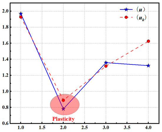
Figure 19. Evolution of early plastic impact response under condition 1.

The new impact factor C₃ is 0.70. The time series of the early plastic strain of the 14-axis measuring point is divided into blocks. Figure 20 illustrates the parameter u of the fitting periodic orbit, as determined using the aforementioned phase space reconstruction method.

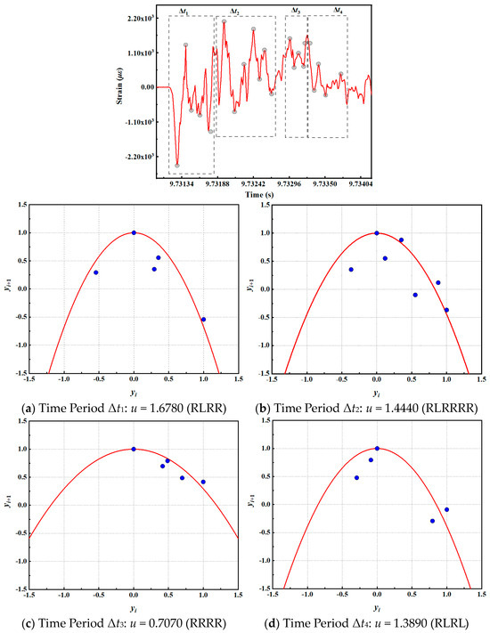
Figure 20. Periodic orbit fitting in different time periods of condition 3.

In the Δt₁ time, the symbol sequence of the periodic orbit of the early plastic impact response is f₁ = RLRR, with u_k = 1.6254 obtained by the word lifting method, and the fitted orbit parameter u is 1.6780. In the Δt₂ time, the symbol sequence of the periodic orbit of the early plastic impact response is f₂ = RLRRRRRR, and the u_k = 1.5749 is obtained. The fitted orbit parameter u is 1.4440. In the time interval Δt₃, the symbol sequence of the periodic orbit of the early plastic impact response is f₃ = RRRR, u_k = 0.7500, and the fitted orbit parameter u is 0.7070. At the time of Δt₄, the symbol sequence of the periodic orbit of the early plastic impact response is f₄ = RLRL, with u_k = 1.2698 obtained. The fitted orbit parameter u is 1.3980. Consequently, when the new impact factor C₃ is 0.70, the early plastic impact response evolution of the measuring point 15 axis is illustrated in Figure 21.

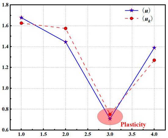
Figure 21. Evolution of early plastic impact response under condition 3.

The new C₃ is 0.70, as determined by the same method. Figure 22 illustrates the early plastic strain signal of the axial direction of measuring point 13, which has been divided into blocks. Table 3 presents the orbital parameters u, u_k of each time series and the corresponding symbol sequence.

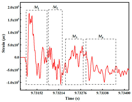
Figure 22. Early axial plastic strain signal at measuring point 13 of condition 3.

Table 3. Measuring point 13 of condition 3.

Time Period	Symbol Sequence	u	uk
Δt1	f1 = RLLRL	1.7893	1.7742
Δt2	f2 = RLLR	1.7986	1.8608
Δt3	f3 = RLRL	1.2480	1.2711
Δt4	f4 = RRRR	0.7070	0.7000

The new impact factor C₃ is 0.70. The early plastic strain signal of the axial direction of measuring point 6 is divided into blocks, as illustrated in Figure 23. The orbital parameters u, u_k of each time series and the corresponding symbol sequence are presented in Table 4.

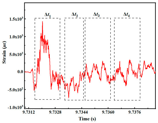
Figure 23. Early axial plastic strain signal at measuring point 6 of condition 3.

Table 4. Measuring point 6 of condition 3.

Time Period	Symbol Sequence	u	uk
Δt1	f1 = RLL	1.9680	1.9408
Δt2	f2 = RRR	0.8210	0.8893
Δt3	f3 = RLRL	1.3580	1.2698
Δt4	f4 = RLRLR	1.2210	1.1659

The new impact factor C₃ is 0.70. The early plastic strain signal of axial direction 15 of the measuring point is divided into blocks, as illustrated in Figure 24. The orbital parameters u, u_k of each time series and the corresponding symbol sequence are presented in Table 5.

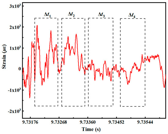
Figure 24. Early axial plastic strain signal at measuring point 15 of condition 3.

Table 5. Measuring point 5 of condition 3.

Time Period	Symbol Sequence	u	uk
Δt1	f1 = RLLRL	1.8360	1.7752
Δt2	f2 = RRRR	0.7500	0.7070
Δt3	f3 = RLRLR	1.2430	1.1659
Δt4	f4 = RLRL	1.3476	1.2698

The unimodal mapping bifurcation diagram, as illustrated in Figure 14, indicates that the symbol sequence and orbital parameters of different measuring points under varying operational conditions exhibit chaotic, periodic, quasi-periodic, and other stages of motion, exhibiting pronounced nonlinear characteristics and non-stationary characteristics. In this context, it is observed that when the ship structure undergoes plastic deformation due to impact load, the impact response signal exhibits baseline drift, the symbol sequence is single, and the periodic orbit parameter value becomes smaller. The symbol sequence of the impact response of the system when the structure undergoes plastic deformation is designated as f* and the orbit parameter is designated as u*. Consequently, the range of f* and u* is as shown in Formula (17).

$$\left\{\begin{array}{l}{f}^{\ast }=RRR\cdots \\ 0.7<u^{\ast }<0.9\end{array}\right.$$

(16)

In conclusion, the symbol sequence f_i = f* and the orbital parameter u_i = u* of the early impact response of the ship experiencing an underwater explosion indicate that the ship structure undergoes plastic deformation. Furthermore, the evolution law of the early nonlinear plastic impact response aligns with the aforementioned characteristics.

6. Verification of Evolution Law of Early Plastic Impact Response

In order to further explore the universality and effectiveness of the phase space mapping method in the analysis of the early plastic impact response evolution law of the underwater explosion ship structure, this paper takes a certain type of ship structure as the prototype to design the model test of the grillage structure and the cabin structure. The early plastic impact response signals of different measuring points are then extracted. The above phase space reconstruction method and symbolic dynamics theory are used to characterize the nonlinear dynamic evolution characteristics of different model tests.

6.1. Ship Grillage Model Test

A single-layer two-way stiffened grillage model is designed under the condition of satisfying the new impact factor C₃, using the grillage of a certain type of ship deck structure as the prototype. The grillage structure is 2 m × 2 m in size, with a 10 mm panel thickness, a grillage material density of 7850 kg/m³, an elastic modulus of 210 GPa, and a Poisson ratio of 0.28. To enhance structural strength, four stiffeners are evenly distributed in the transverse and longitudinal directions of the plate frame. The charge is placed between the pontoon and the stiffened plate frame structure in the form of hoisting, and the charge is perpendicular to the stiffened plate frame structure. The explosion distance is the vertical distance between the target plate and the centroid of the charge. The charge is made of TNT, with a mass of 8 kg and an impact coefficient of 0.97. The 3D scanning diagram of the plate frame model and the layout diagram of the test site are presented in Figure 25 and Figure 26, respectively.

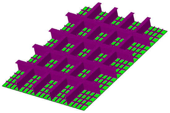
Figure 25. Three-dimensional scanning diagram of single-layer two-way stiffened plate frame model.

Figure 26. Layout diagram of the test.

The back empty water tank is designed to provide an empty rear environment for the plate frame. The gravel tank is located beneath the back empty water tank, and the counterweight block is positioned to increase the weight of the back empty water tank and shift its center of gravity downward, thereby preventing the back empty water tank from overturning due to disturbances in the water. In the test, four wire ropes are utilized to connect the buoy and the backwater sump. The double buoy is then floated on the surface of the water, providing buoyancy for the entire system. The backwater sump is placed underwater, and a damping plate is installed to reduce the sagging of the system and stabilize the rigid body displacement of the system. The plate frame structure is fixed to the target support of the backwater sump by bolts, and the explosive is hoisted directly above the plate frame by flexible rope. Figure 27 illustrates the test system.

Figure 27. Scale model test system of plate frame.

The operability of strain gauges is considered in order to determine the local strength of strain measuring points. Figure 28 illustrates the arrangement of strain measuring points on the plate frame. A measuring point is arranged every 200 mm in the x-axis, numbered from 1 to 5; similarly, a measuring point is arranged every 200 mm in the y-axis, numbered from 1 to 5. E-ab represents the measurement position of the strain, where a is the x-axis position number and b is the y-axis position number.

Figure 28. Position of strain measuring points on the plate.

The early plastic strain signals of measuring points E11, E12, E14, E16, E44 and E55 are analyzed as an example, as shown in Figure 29.

Figure 29. Strain signals at different measuring points of the plate frame. (a) Strain signal of measuring points E11. (b) Strain signal of measuring points E12. (c) Strain signal of measuring points E14. (d) Strain signal of measuring points E16. (e) Strain signal of measuring points E44. (f) Strain signal of measuring points E55.

From the strain signals of the aforementioned measuring points, it can be observed that under the early impact load, the plate frame structure exhibits considerable plastic deformation, and the early impact response signal exhibits a baseline drift with a pronounced trend, which affects the symbol sequence and track parameters of the early plastic impact response. Table 6 presents the track parameter u* when plastic deformation occurs at different measuring points.

Table 6. Track parameter u* of different measuring points of plate frame.

Measuring Point	Symbol Sequence f*	Track Parameter u*
E11	RRRR	0.7070
E12	RRRR	0.7070
E14	RRR	0.8893
E16	RRRR	0.7070
E44	RRR	0.8893
E55	RRRR	0.7070

6.2. Ship Cabin Model Test

A 1:1.5 cabin model was designed based on a specific type of ship cabin structure. The charge is made of TNT, with a mass of 2.3 kg, and the new impact factor C3 was set at 2.43. The cabin structure was 2.8 m long, 1.67 m high, 0.33 m above the water line, and 1.13 m wide. The material density is 7800 kg/m³, the elastic modulus is 210 GPa, and the Poisson ratio is 0.3. The model extends two cabins outward and sets horizontal baffles and vertical baffles to restrict the rigid body motion in the horizontal and vertical directions, respectively. The model test was carried out in the explosion pool. The explosive was vertically hoisted beneath the water surface, parallel to the outer surface of the cabin, with a water depth of 0.83 m, as illustrated in Figure 30 and Figure 31.

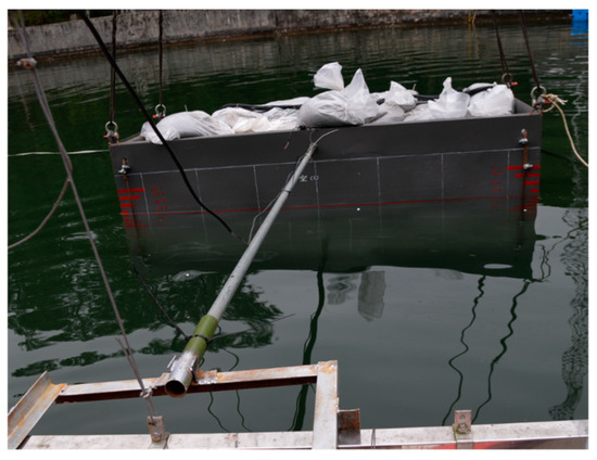
Figure 30. Layout diagram of cabin model test.

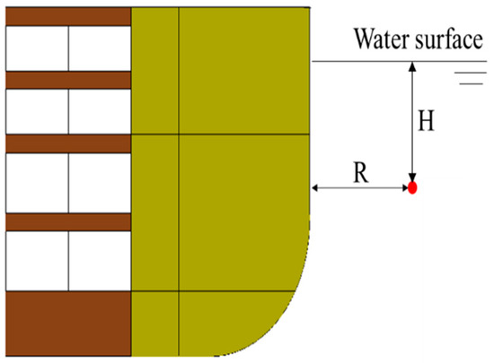
Figure 31. Charging arrangement diagram of cabin model test.

Three measuring points in the same horizontal direction, each located at a different cabin center on the deck of the cabin structure, are selected as strain measuring points. The position of each measuring point is illustrated in Figure 32.

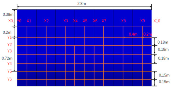
Figure 32. Diagram of measuring point arrangement in the cabin model test.

The early plastic strain signals of measuring points X1, X2, and X3 are utilized as exemplars for analysis, as illustrated in Figure 33.

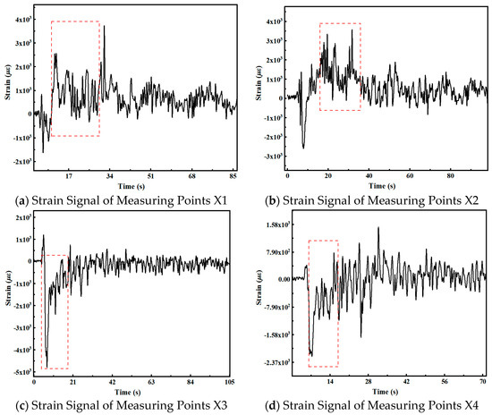
Figure 33. Strain signals of different measuring points in the cabin section.

Table 7 presents the symbol sequence f* and the orbital parameter u* when plastic deformation occurs at the aforementioned measuring points. The orbital parameter of the plastic stage is about 0.8, which describes the evolution law of early plastic impact response. This indicates that early plastic impact response has strong nonlinear and non-stationary characteristics.

Table 7. Track parameters u* of different measuring points in the cabin section.

Measuring Point	Symbol Sequence f*	Track Parameters u*
X1	RRRRR	0.7556
X2	RRRR	0.7070
X3	RRR	0.8893
X4	RRRR	0.7070

7. Conclusions

This paper examines the nonlinear dynamic response of a typical underwater explosion ship structure. It employs phase space reconstruction technology, parabolic mapping methods, and symbolic dynamics theory to analyze the plastic strain response signal, which exhibits high frequency, severe amplitude change, and strong randomness in the occurrence of plastic deformation. By designing model tests under different impact factors, the phase space reconstruction of the strain response of typical ship structures when plastic deformation occurs was carried out. The system motion trajectory was characterized by the data trajectory in the phase space, and the evolution law of the nonlinear system was described. The following conclusions were obtained:

(1)

The dynamic response of underwater explosion ship structures can be divided into two stages: the transient early impact response stage and the late impact response stage. The random characteristics of large amplitude, high frequency, short duration, and drastic changes in the early transient impact response stage are one of the important factors leading to plastic deformation of the structure.

(2)

The nonlinear dynamic data analysis method based on phase space reconstruction technology, parabolic mapping, and symbolic dynamics theory can be used to describe the motion trajectory of early plastic impact dynamic response, achieving quantitative characterization of the evolution law of early plastic impact dynamic response of underwater explosion ship structures.

(3)

The self similarity scale-free range of different early plastic impact response signals varies, with characteristic lengths ranging from 10 to 20 times the pulse width of the incident shock wave.

(4)

Based on the scale-free range of the response signal, the early plastic impact response signal is segmented, and it is concluded that the early plastic impact response exhibits various dynamic behaviors such as chaotic motion, periodic motion, and quasi-periodic motion. The orbital parameter of the plastic stage is about 0.8, which describes the evolution law of early plastic impact response. This indicates that early plastic impact response has strong nonlinear and non-stationary characteristics.

References

- Barras, G.; Souli, M.; Aquelet, N.; Couty, N. Numerical simulation of underwater explosions using an ALE method. The pulsating bubble phenomena. Ocean Eng. 2012, 41, 53–66. [Google Scholar] [CrossRef]
- He, Z.; Chen, Z.; Jiang, Y.; Cao, X.; Zhao, T.; Li, Y. Effects of the standoff distance on hull structure damage subjected to near-field underwater explosion. Mar. Struct. 2020, 74, 13. [Google Scholar] [CrossRef]
- Pan, X.; Wang, G.; Lu, W.; Yan, P.; Chen, M.; Gao, Z. The effects of initial stresses on nonlinear dynamic response of high arch dams subjected to far-field underwater explosion. Eng. Struct. 2022, 256, 21. [Google Scholar] [CrossRef]
- Liu, Y.; Zhang, A.; Tian, Z.; Wang, S. Numerical investigation on global responses of surface ship subjected to underwater explosion in waves. Ocean Eng. 2018, 161, 277–290. [Google Scholar] [CrossRef]
- Jen, C.; Lai, W. Transient response of multiple intersecting spheres of deep-submerged pressure hull subjected to underwater explosion. Theor. Appl. Fract. Mech. 2007, 48, 112–126. [Google Scholar] [CrossRef]
- Zheng, Z.; Ruan, L.; Zhu, M. Output-constrained tracking control of an underactuated autonomous underwater vehicle with uncertainties. Ocean Eng. 2019, 175, 241–250. [Google Scholar] [CrossRef]
- Wang, J.; Wang, C.; Wei, Y.; Zhang, C. Filter-backstepping based neural adaptive formation control of leader-following multiple AUVs in three dimensional space. Ocean Eng. 2020, 201, 11. [Google Scholar] [CrossRef]
- Shu, Y.; Wang, G.; Lu, W.; Chen, M.; Lv, L.; Chen, Y. Damage characteristics and failure modes of concrete gravity dams subjected to penetration and explosion. Eng. Fail. Anal. 2022, 134, 20. [Google Scholar] [CrossRef]
- Liu, B.; Peng, J. Nonlinear Dynamics; Higher Education Press: Beijing, China, 2004. [Google Scholar]
- Xing, L.; Lin, H.-R.; Zhang, D.; Li, Q.-Q.; Zhou, H.-W.; Liu, H.-S. Facial characteristics of air gun array wavelets in the time and frequency domain under real conditions. J. Appl. Geophys. 2022, 199, 104591. [Google Scholar] [CrossRef]
- Colicchio, G.; Greco, M.; Brocchini, M.; Faltinsen, O.M. Hydroelastic behaviour of a structure exposed to an underwater explosion. Philos. Trans. R. Soc. A Math. Phys. Eng. Sci. 2015, 373, 20140103. [Google Scholar] [CrossRef]
- Shan, F.; He, Y.; Jiao, J.-J.; Wang, H.-C. Experimental and theoretical analysis of detonation products state on bubble dynamics and energy distribution in underwater explosion. J. Appl. Phys. 2021, 130, 174701. [Google Scholar] [CrossRef]
- Liu, Z.; Qian, D.; Xu, C.; Li, L.; Zou, X.; Wang, X. Unbalanced distribution of electric current in underwater electrical wire array explosion. J. Phys. D Appl. Phys. 2022, 55, 185205. [Google Scholar] [CrossRef]
- Ruzzo, C.; Arena, F. A numerical study on the dynamic response of a floating spar platform in extreme waves. J. Mar. Sci. Technol. 2018, 24, 1135–1152. [Google Scholar] [CrossRef]
- Li, J.; Qi, H.; Wang, S.; Wang, X.; Jie, Z. Hydrological meaning and applications of phase space reconstruction of runoff series. Water Resour. Prot. 2024, 40, 90–97. [Google Scholar] [CrossRef]
- Cao, L. Practical method for determining the minimum embedding dimension of a scalar time series. Phys. D Nonlinear Phenom. 1997, 110, 43–50. [Google Scholar] [CrossRef]
- Huang, F.; Yin, K.; Zhang, G.; Gui, L.; Yang, B.; Liu, L. Landslide displacement prediction using discrete wavelet transform and extreme learning machine based on chaos theory. Environ. Earth Sci. 2016, 75, 18. [Google Scholar] [CrossRef]
- Hao, B.; Zheng, W. Practical Symbolic Dynamics and Chaos; Peking University Press: Beijing, China, 2014. [Google Scholar]
- Hao, B. Introduction to Chaos Dynamics; Shanghai Science and Technology Education Press: Shanghai, China, 1993. [Google Scholar]
- Zheng, W.; Hao, B. Practical symbolic dynamics. Adv. Phys. 1990, 10, 58. [Google Scholar]
- Jin, Q.K.; Ding, G.Y. A finite element analysis of ship sections subjected to underwater explosion. Int. J. Impact Eng. 2011, 38, 558–566. [Google Scholar] [CrossRef]
- Wang, J.; Yao, X.; Yang, D. Impact analysis of shock environment from floating shock platform on equipment response. Explos. Shock 2015, 35, 236–242. [Google Scholar]
- Yao, X.; Zhao, K.; Shi, D. Study on the effectiveness of impact factor in underwater explosion model test. Int. J. Impact Eng. 2023, 185, 13. [Google Scholar] [CrossRef]
- Han, W.; Dong, Y.; Li, R.; Nan, H.; Zhang, Y.; Bai, L. Damage mechanisms of underwater explosive bubble on water-filled bilayer spherical shells during navigation. Ocean Eng. 2024, 306, 118113. [Google Scholar] [CrossRef]
- Xue, Z.-Q.; Li, S.; Xin, C.-L.; Shi, L.-P.; Wu, H.-B. Modeling of the whole process of shock wave overpressure of free-field air explosion. Def. Technol. 2019, 15, 815–820. [Google Scholar] [CrossRef]
- Yang, H.; Fang, L.; He, W. Study of correlation dimension on EEG. J. Biomed. Eng. 2004, 21, 81–84. [Google Scholar]
- Kumar, S.; Hamid, I.; Abdou, M.A. Dynamic frameworks of optical soliton solutions and soliton-like formations to Schrodinger-Hirota equation with parabolic law non-linearity using a highly efficient approach. Opt. Quantum Electron. 2023, 55, 31. [Google Scholar] [CrossRef]
Disclaimer/Publisher’s Note: The statements, opinions and data contained in all publications are solely those of the individual author(s) and contributor(s) and not of MDPI and/or the editor(s). MDPI and/or the editor(s) disclaim responsibility for any injury to people or property resulting from any ideas, methods, instructions or products referred to in the content. |
© 2025 by the authors. Licensee MDPI, Basel, Switzerland. This article is an open access article distributed under the terms and conditions of the Creative Commons Attribution (CC BY) license (https://creativecommons.org/licenses/by/4.0/).