Article

Design of an Experimental Teaching Platform for Flow-Around Structures and AI-Driven Modeling in Marine Engineering

1
Ocean College, Zhejiang University, Zhoushan 316021, China
2
Department of Applied Mathematics and Mathematical Modeling, Saint Petersburg State Marine Technical University, Saint Petersburg 190121, Russia
*
Author to whom correspondence should be addressed.
J. Mar. Sci. Eng. 2025, 13(9), 1761; https://doi.org/10.3390/jmse13091761
Submission received: 15 August 2025 / Revised: 3 September 2025 / Accepted: 8 September 2025 / Published: 11 September 2025

Abstract

Flow past bluff bodies (e.g., circular cylinders) forms a canonical context for teaching external flow separation, vortex shedding, and the coupling between surface pressure and hydrodynamic forces in offshore engineering. Conventional laboratory implementations, however, often fragment local and global measurements, delay data feedback, and omit intelligent modeling components, thereby limiting the development of higher-order cognitive skills and data literacy. We present a low-cost, modular, data-enabled instructional hydrodynamics platform that integrates a transparent recirculating water channel, multi-point synchronous circumferential pressure measurements, global force acquisition, and an artificial neural network (ANN) surrogate. Using feature vectors composed of Reynolds number, angle of attack, and submergence depth, we train a lightweight AI model for rapid prediction of drag and lift coefficients, closing a loop of measurement, prediction, deviation diagnosis, and feature refinement. In the subcritical Reynolds regime, the measured circumferential pressure distribution for a circular cylinder and the drag and lift coefficients for a rectangular cylinder agree with empirical correlations and published benchmarks. The ANN surrogate attains a mean absolute percentage error of approximately 4% for both drag and lift coefficients, indicating stable, physically interpretable performance under limited feature inputs. This platform will facilitate students’ cross-domain transfer spanning flow physics mechanisms, signal processing, feature engineering, and model evaluation, thereby enhancing inquiry-driven and critical analytical competencies. Key contributions include the following: (i) a synchronized local pressure and global force dataset architecture; (ii) embedding a physics-interpretable lightweight ANN surrogate in a foundational hydrodynamics experiment; and (iii) an error-tracking, iteration-oriented instructional workflow. The platform provides a replicable pathway for transitioning offshore hydrodynamics laboratories toward an integrated intelligence-plus-data literacy paradigm and establishes a foundation for future extensions to higher Reynolds numbers, multiple body geometries, and physics-constrained neural networks.

1. Introduction

Flow past circular cylinders and other bluff bodies has long constituted a canonical case for fluid mechanics research and instruction owing to its ubiquity in offshore engineering, wind energy development, and transportation systems [1,2,3]. Classical boundary-layer theory, together with systematic elucidation of flow separation, reattachment, and vortex shedding mechanisms, furnishes an analytical framework for interpreting drag decomposition, lift fluctuations, and associated energy exchange. Extensive experimental and computational investigations have characterized, across steady and unsteady regimes, the formation of Kármán vortex streets, frequency locking phenomena, and the evolution of coherent structures [4,5,6], thereby underpinning drag-reduction and vibration-mitigation strategies in engineering design. Concurrently, advances in high-resolution diagnostics and large-scale simulation continue to expand the dimensionality and volume of bluff-body flow datasets. This escalation introduces a pedagogical challenge: enabling students to efficiently bridge localized field measurements with global hydrodynamic (aerodynamic) responses.
Conventional undergraduate and graduate fluid mechanics laboratories typically center on a single measurement modality (e.g., differential pressure tapping or a drag balance), with learning objectives often confined to reproducing a canonical curve. This narrow focus fragments conceptual understanding and limits higher-order cognition—namely cross-scale integration, model abstraction, and synthesis of data-driven methodologies [7]. The prevailing format is misaligned with contemporary engineering education priorities emphasizing active learning and evidence-based deep engagement [8,9], and it falls short of the competency profile of interdisciplinary breadth coupled with data literacy articulated within the national “New Engineering” framework [10,11]. Internationally, convergent integration of data assimilation, machine learning, and physics-based modeling for flow prediction, state estimation, and reduced-order representation has become mainstream [12,13,14]. Recent advances in applying machine learning to turbulence closure modeling, feature extraction, and real-time forecasting demonstrate that embedding physical priors markedly mitigates overfitting and reduces extrapolation risk [15,16,17]. Nevertheless, a replicable instructional paradigm is still lacking for embedding coordinated, data-driven, and physics-interpretable learning activities into low-cost, open platforms under resource constraints.
Current instructional experiments on bluff-body (cross-flow) aerodynamics/hydrodynamics commonly suffer from the following three representative limitations: (i) lack of temporal synchrony between local measurements and global force data, impeding student validation of force estimates via pressure integration and obscuring rigorous error attribution; (ii) delayed data feedback, which constrains inquiry-oriented learning driven by immediate predictive hypotheses; and (iii) a structural disconnect between “intelligent” modeling modules and the physical experiment, depriving learners of an end-to-end workflow spanning raw signal conditioning, feature engineering, and model evaluation. To bridge these gaps, we introduce an integrated “multi-point pressure–three-component force (Fx, Fy, and Fz)–lightweight ANN” platform. A circumferential array of pressure taps acquires the instantaneous surface pressure distribution, while a three-component balance supplies synchronized global force data, establishing a local–global closure loop. A compact input vector built from core physical descriptors (Reynolds number, angle of attack, immersion depth) trains a lightweight artificial neural network to predict drag and lift coefficients CD and CL; juxtaposition with measured coefficients drives an iterative prediction–discrepancy–diagnosis–refinement cycle. Relative to high-cost wind tunnels or full-field PIV systems, the proposed platform prioritizes cost controllability and pedagogical portability, enabling learners under resource constraints to engage with multimodal data fusion and cultivate data-driven, physics-informed reasoning.
This study makes the following three primary contributions:
  • We establish, in an instructional setting, a synchronized data schema coupling circumferential surface pressure measurements with three-component force records (Fx, Fy, and Fz). This integration enables validation that links local pressure coefficients to a drag (force) decomposition pathway and sharpens students’ quantitative understanding of boundary-layer separation effects.
  • We design a lightweight ANN prediction framework that fuses physically interpretable descriptors (e.g., Reynolds number, angle of attack, and immersion depth) with data-driven inference, thereby articulating a pedagogical pathway for data–model–physics triadic synergy consistent with emerging trends in intelligent fluid mechanics [18,19,20].
  • We detail low-cost hardware implementations and a modular expansion strategy, furnishing a realistic springboard for future scaling to higher Reynolds number regimes, broader families of body geometries, and physics-constrained neural paradigms (e.g., PINNs) [21,22,23].
Paper structure is as follows: Section 2 outlines the platform architecture, sensor topology, and acquisition pipeline. Section 3 describes experimental analysis and the data-driven modeling workflow, including feature engineering and network design. Section 4 presents surface pressure distributions, hydrodynamic force/coefficients, and ANN predictive metrics. Section 5 examines measurement fidelity, error sources, model limitations, and pedagogical implications. Section 6 concludes and discusses prospective extensions toward high-Re applications and hybrid physics-informed modeling.

2. Overall Platform Architecture

2.1. Design of the Experimental Apparatus

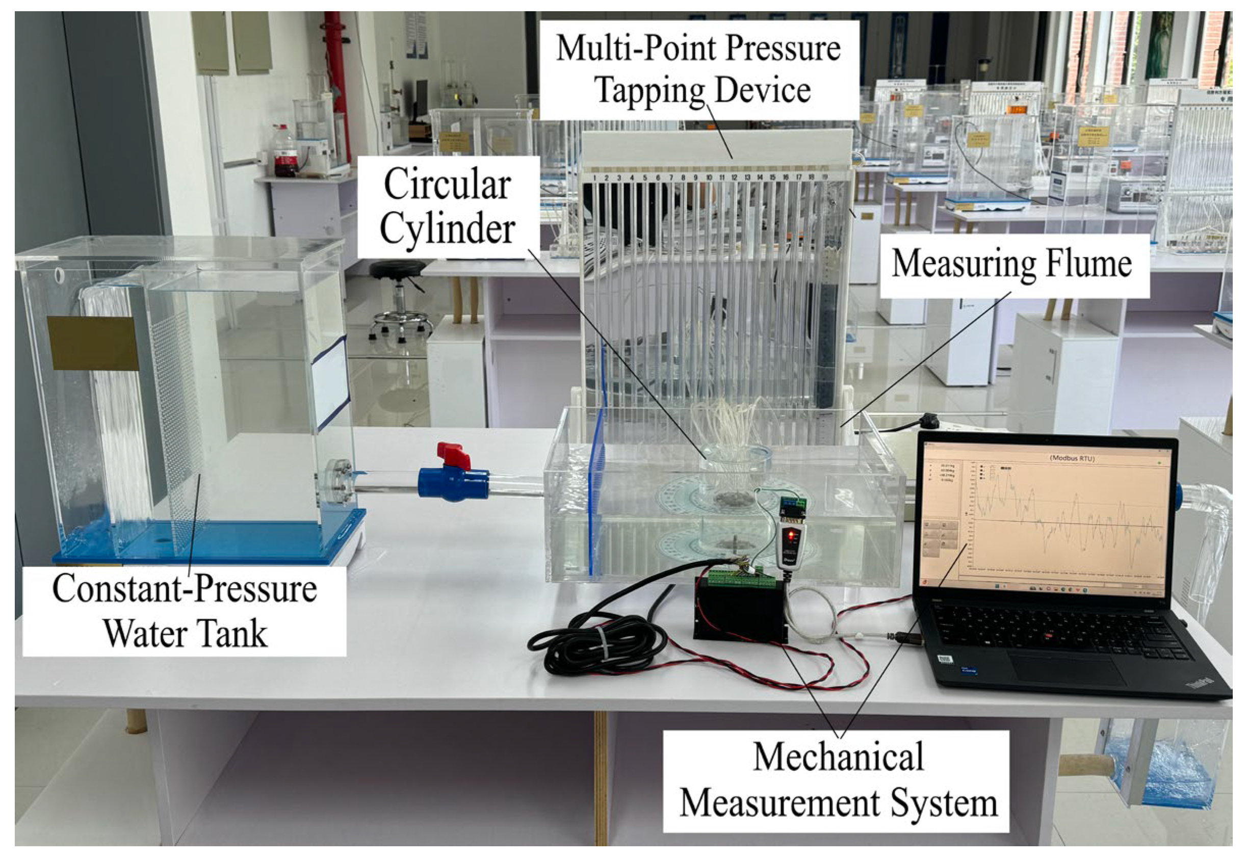
The apparatus was purpose-built to support instructional investigation and research on bluff-body/external flow phenomena. It combines a compact footprint with integrated functionality and operator-friendly maintenance. The system comprises the following: (i) a closed-loop (self-circulating) water supply subsystem; (ii) a measurement/test section (tank) providing optical and physical access; (iii) an interchangeable test article; (iv) a multi-channel pressure acquisition module for circumferential surface pressure sampling; and (v) a three-component force sensor enabling synchronized global load measurements. A schematic/photograph of the overall configuration is presented in Figure 1.
As illustrated in Figure 1, the recirculating water system comprises a submersible pump, a supply reservoir, a constant-head tank, and interconnecting piping. Flow delivered by the pump enters the constant-head tank, where an overflow weir and a flow-straightening baffle (plate A) partition the interior into multiple chambers, damping free-surface fluctuations and stabilizing discharge. Once the constant-head level is established (continuous overflow), the inlet valve is trimmed to direct water through the feed line into the test (measurement) tank. After passing around the test article, the stream exits via the outlet valve into a return tank and ultimately drains back to the supply reservoir, forming a closed-loop, self-circulating circuit. This configuration conserves water and supports long-duration and repeated instructional experiments. Independent inlet and outlet valve control permits adjustment of both bulk flow rate and water depth to suit differing test conditions.
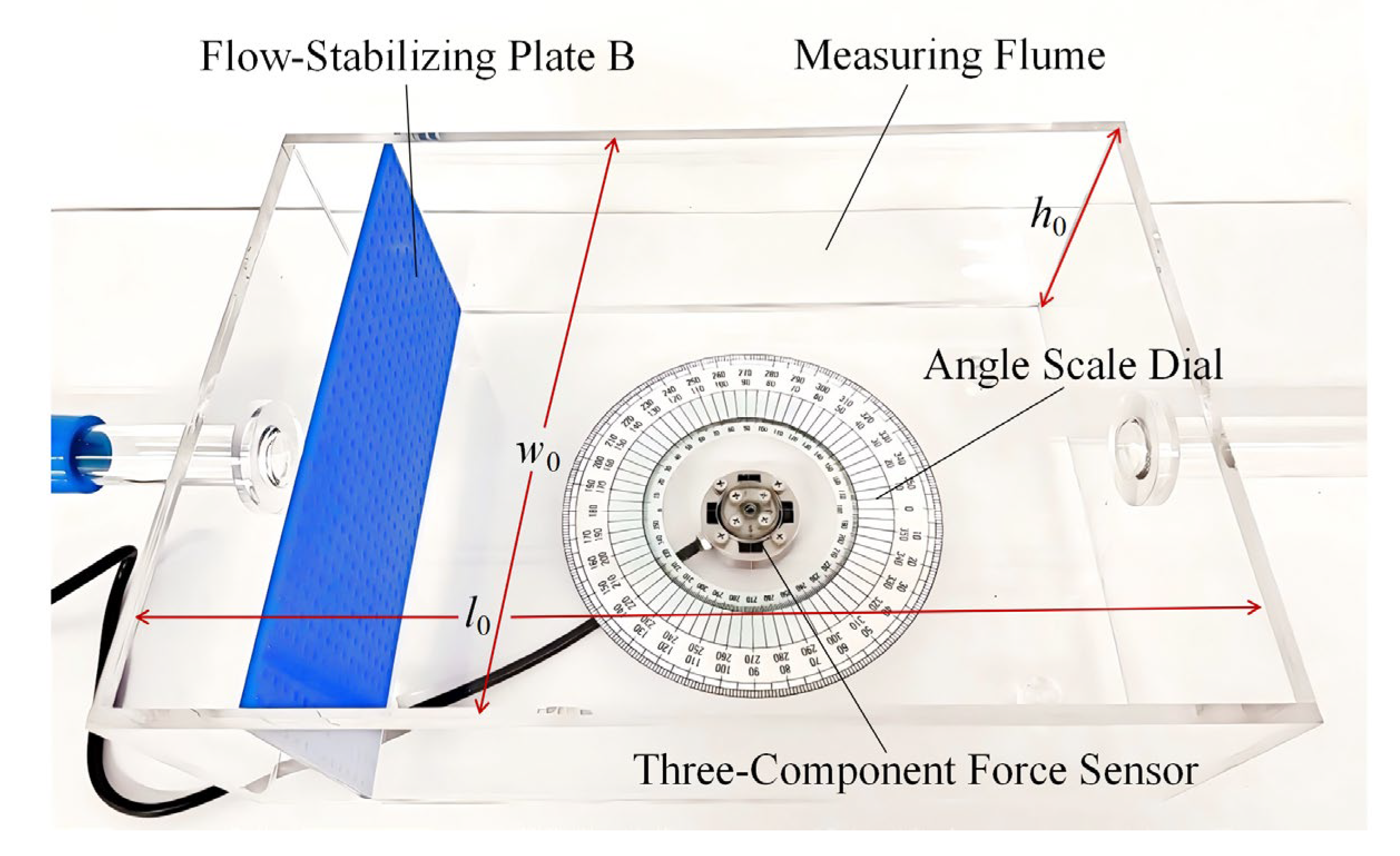
The measurement tank is an open-top, transparent rectangular acrylic (PMMA) enclosure enabling real-time visualization of the external flow and near-surface unsteady features. A central primary mounting bore plus four auxiliary locating holes on the base plate ensure precise alignment and rigid fixation of the three-component force sensor. A circumferentially mounted, graduated angular scale (protractor ring) provides accurate setting and logging of the model angle of attack. Leveling feet allow fine planar adjustment, mitigating systematic bias induced by residual tilt. To condition the inflow and attenuate turbulence intensity, a second flow-straightening element (plate B) is installed upstream within the inlet section. Consistent with sidewall interference mitigation guidelines, the ratio of tank width to model width exceeds 4, limiting lateral blockage and preserving core-flow uniformity, thereby enhancing the fidelity of both force and pressure/flow measurements. In this experiment, the flume length, width, and water depth were l0 = 750 mm, w0 = 500 mm, and h0 = 150 mm, respectively. A photograph (Figure 2) documents the physical test section.
The initial test article is a hollow, transparent acrylic (PMMA) cylinder with a smooth exterior surface to minimize skin-friction drag; alternative model geometries can be substituted as required by subsequent experimental objectives. The cylinder is rigidly affixed to the three-component force transducer mounted in the floor of the measurement tank, using either bolted fastening or structural adhesive, ensuring zero perceptible displacement or loosening over the test duration. In the multi-point pressure measurement system, 24 through-hole pressure taps (2 mm in diameter) were drilled on the same circumferential plane of the cylinder sidewall at 15° angular intervals; 19 of these taps were connected in a prescribed sequence via flexible tubing to 19 manometer tubes, while the remaining taps were left unused, and these 19 measurement points sufficiently cover the semicylindrical region. All piezometric tubes are mounted plumb on a support frame equipped with a laterally translatable (sliding) scale, enabling direct reading of the water column height in each tube. These readings yield the local static pressure at each tap, permitting both visualization and quantitative mapping of the circumferential surface pressure distribution. The piezometer tube has an inner diameter of 1 cm, and a rear-mounted reflective mirror is employed to effectively eliminate parallax. During manual readings, the tube is kept strictly vertical, the observer’s line of sight is aligned with the meniscus, and a calibrated scale is used, allowing the measurement precision to be consistently maintained within ±0.2 mm. Figure 3 presents the fabricated cylinder together with the multi-point pressure measurement assembly. In this experiment, the cylinder had an outer diameter D = 70 mm and a height H0 = 120 mm.
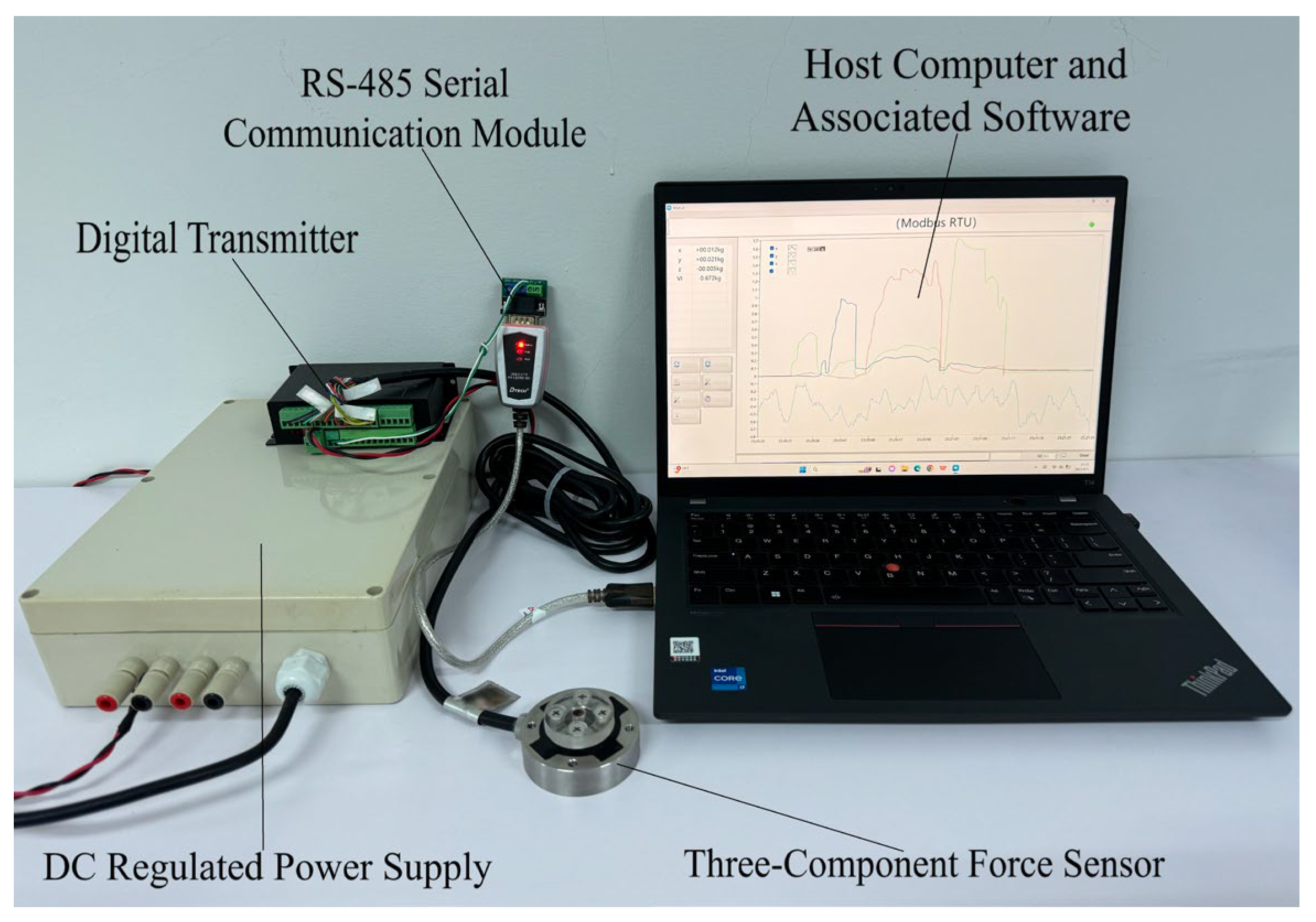
A three-component force transducer mounted on the floor of the measurement tank acquires the model’s streamwise drag and vertical lift in real time. These force measurements complement the surface pressure data, enabling quantitative characterization of the temporal evolution and parametric trends of both drag and lift. The instrumentation chain comprises the three-component force transducer, a regulated DC power supply, a digital transmitter, an RS-485 communication interface module, and a host computer running bespoke acquisition software. The transducer’s low-level analog outputs are conditioned and converted to a standard digital data stream, which is transmitted in real time to the computer for continuous acquisition, visualization, and monitoring. The three-component force transducer was factory calibrated, and the corresponding calibration coefficients were imported into the test software prior to measurement. Although the detailed calibration procedure is not reported herein, subsequent verification using laboratory standard weights confirmed that the measurement error remained within 2%. The resulting high-resolution, time-synchronized force dataset establishes a robust foundation for subsequent theoretical analysis and AI-based modeling. Figure 4 presents the force measurement system.

2.2. Experimental Procedure

The experiment is designed to integrate qualitative visualization with quantitative measurement. By jointly acquiring surface pressure distributions and resultant drag and lift, it enables students to internalize fundamental external-flow concepts and the physical mechanisms underlying aerodynamic (hydrodynamic) force generation, thereby strengthening both the investigative depth and hands-on engagement of the instructional laboratory. To aid comprehension of the spatial arrangement and functional interrelationships among subsystems, an overall photograph of the complete apparatus is provided (Figure 5).
The detailed experimental methodology is presented below.
Prior to each run, all mechanical and fluid connections were inspected for rigidity and leaks; manometer tubes and flexible hoses were verified to be airtight, and the three-component force transducer was zeroed. The cylindrical test model was then secured to the transducer, ensuring sealed communication between its circumferential pressure taps and the connecting hoses. Before commencing measurements, the flume was repeatedly filled, circulated, and refreshed, then allowed to stand to promote passive degassing of dissolved gases. Each piezometric line was purged individually with a rubber air bulb to remove any residual bubbles, thereby preserving pressure measurement accuracy. After the submersible pump was started and overflow from the constant-head tank was established, the valves were adjusted to introduce a stable flow into the test section.
A steady external flow past the cylinder was maintained by fine regulation of the upstream and downstream valves. Static pressure at discrete circumferential locations was conveyed from the sidewall pressure taps, through the hoses, to a multi-tube manometer bank. After liquid columns became quiescent, individual heights were recorded to determine local surface pressures. Concurrently, the three-component force transducer acquired time histories of drag and lift. Parametric studies were enabled by substituting alternative body geometries and varying bulk velocity, water depth, and angle of attack to elucidate their effects on wake development and force characteristics. In this experiment, the volumetric flow rate of water was determined using a gravimetric (weighing) method with a measurement interval of 10 s. After allowing the flow to reach a steady state, an empty container was placed on an electronic balance (resolution 0.1–1 g) and tared. The water inflow and the timer were then started and stopped synchronously, while splashing was minimized and the exterior wall of the container kept dry. The mass increase over the 10 s interval was recorded and converted to volumetric flow rate, yielding a combined measurement uncertainty controlled within ±0.5%. The average bulk flow velocity was subsequently obtained by dividing the measured volumetric flow rate by the effective cross-sectional area of the test section.
Data reduction proceeded by converting manometer readings into surface pressure values and mapping the pressure distribution. These results were coupled with the measured forces to examine trends in drag and lift and to compare them with theoretical expectations. The theoretical drag was computed using Bernoulli relationships and the standard drag coefficient formulation, enabling quantitative error assessment and refinement of conceptual understanding of bluff-body (or external) flow physics.
Operational discipline emphasized the following: (i) maintaining a constant flow rate; (ii) excluding air bubbles from pressure lines; and (iii) re-zeroing the force transducer and re-checking all seals after any change in model or test condition. Ambient and fluid parameters (e.g., water temperature and approach velocity) were logged to support subsequent corrections (e.g., density/viscosity adjustment) and systematic uncertainty analysis.

3. Methodology

3.1. Surface Pressure Distribution: Theory and Experiment

The surface pressure distribution of a body in crossflow provides a key indicator of its flow characteristics. For an ideal (inviscid, incompressible, and irrotational) flow past a circular cylinder, the pressure at any point on the surface can be obtained from the Bernoulli equation combined with potential-flow theory. The surface pressure coefficient is given by the following expression:
C P = 2 ( P θ P 0 ) ρ U 0 2 = 1 4   sin 2   θ
where CP denotes the surface pressure coefficient of the circulardenotes the surface pressure coefficient of the circular cylinder; θ is the polar angle measured along the cylinder surface from the forward (upstream) stagnation point to the measurement location; Pθ is the static pressure at the surface point corresponding to angle θ; P0 is the undisturbed free-stream static pressure; ρ is the fluid density; and U0 is the free-stream velocity. Theoretically, the pressure distribution over the cylinder surface is fore–aft symmetric, with the maximum pressure occurring at the forward stagnation point. However, in the actual flow, viscous effects and boundary-layer separation cause a pronounced pressure deficit downstream of the separation point, leading the measured distribution to deviate substantially from the ideal potential-flow prediction.
To investigate in greater depth the surface pressure distribution characteristics of flow around a circular cylinder, a hollow cylinder with an outer diameter of 70 mm, a height of 120 mm, and a wall thickness of 6 mm was employed. Pressure taps (through-holes) of 2 mm diameter were located at the mid-span (mid-height) of the cylinder. Considering the symmetry of the flow around a non-rotating circular cylinder, it is sufficient to focus on the pressure distribution over a semicylindrical region. By utilizing 13 consecutive through-holes on the cylinder, pressures at all required stations from the forward stagnation point to the rear stagnation vicinity can be obtained, as illustrated in Figure 6a; the initially indexed 13 holes correspond to measurement locations in the range θ = 0–180°. The cylinder is then rotated clockwise by 10° and re-fixed so that the same 13 holes correspond to θ = 10–190°, as shown in Figure 6b. By repeating this indexed rotation procedure sequentially, pressure at any circumferential position within θ = 0–360° can be measured. This strategy effectively enhances the angular (azimuthal) resolution and measurement coverage of the pressure taps. The acquired pressure data enable direct identification of key flow features such as the separation point and the extent of the wake (recirculation) region. The resulting CP distribution supplies experimental support for validating the theoretical model and helps students develop a deeper understanding of the influence of viscosity and boundary-layer separation on the flow.

3.2. Theoretical and Experimental Analysis of Drag and Lift

For a body in relative motion through a fluid, the total aerodynamic drag consists principally of pressure (form) drag and skin-friction drag. In the case of flow past a circular cylinder (typical bluff body), pressure drag overwhelmingly dominates. The drag coefficient, a dimensionless measure of the resistance force, is defined by the following expression:
C D = 2 F D ρ U 0 2 A
where CD is the drag coefficient, FD the total drag force on the body, and A the frontal (projected) reference area. By D’Alembert’s paradox, an ideal (inviscid, incompressible, irrotational) and fully attached potential flow over a smooth circular cylinder would yield zero theoretical drag. The nonzero drag measured experimentally is instead attributable chiefly to viscous dissipation together with separation-induced wake (vortex shedding) dynamics. The Reynolds number Re, which controls the flow regime and thus the level of CD, is given by the following expression:
R e = U 0 D ν
where D denotes the cylinder outer diameter and ν the kinematic viscosity. For Re < 1, the flow resides in the viscous (creeping/Stokes) regime: a symmetric laminar pattern without a separated, recirculating wake. In this limit, CD is given by Equation (4).
C D = 24 R e
For 102 < Re < 105 (subcritical regime), the boundary layer stays laminar over the forward face and separates relatively early, yielding an unsteady Kármán vortex street in the wake and a drag coefficient of roughly CD ≈ 1. Once Re > 2 × 10⁵ (supercritical regime), boundary-layer transition triggers delayed separation; the wake contracts, pressure recovery strengthens, and CD declines rapidly to approximately 0.3–0.5.
Lift is defined as the component of the aerodynamic (hydrodynamic) force on the test article that is perpendicular to the free-stream velocity vector, and it typically arises from geometric asymmetry and/or a nonzero angle of attack. The lift coefficient is given by the following expression:
C L = 2 F L ρ U 0 2 A
where CL denotes the lift coefficient and FL the lift force on the body. For an ideal symmetric configuration—zero angle of attack, no rotation, and absence of any geometric or flow asymmetry—the circular cylinder should generate zero lift. In practice, instructional (teaching) experiments can exhibit small instantaneous fluctuations or a weak nonzero mean lift caused by slight mounting misalignment, inflow non-uniformity, or transient asymmetries in the Kármán vortex street. By enforcing a highly uniform free stream and ensuring precise fixture alignment, the present experimental platform suppresses such biases to a negligible level, thereby isolating and highlighting drag as the primary phenomenon of interest.
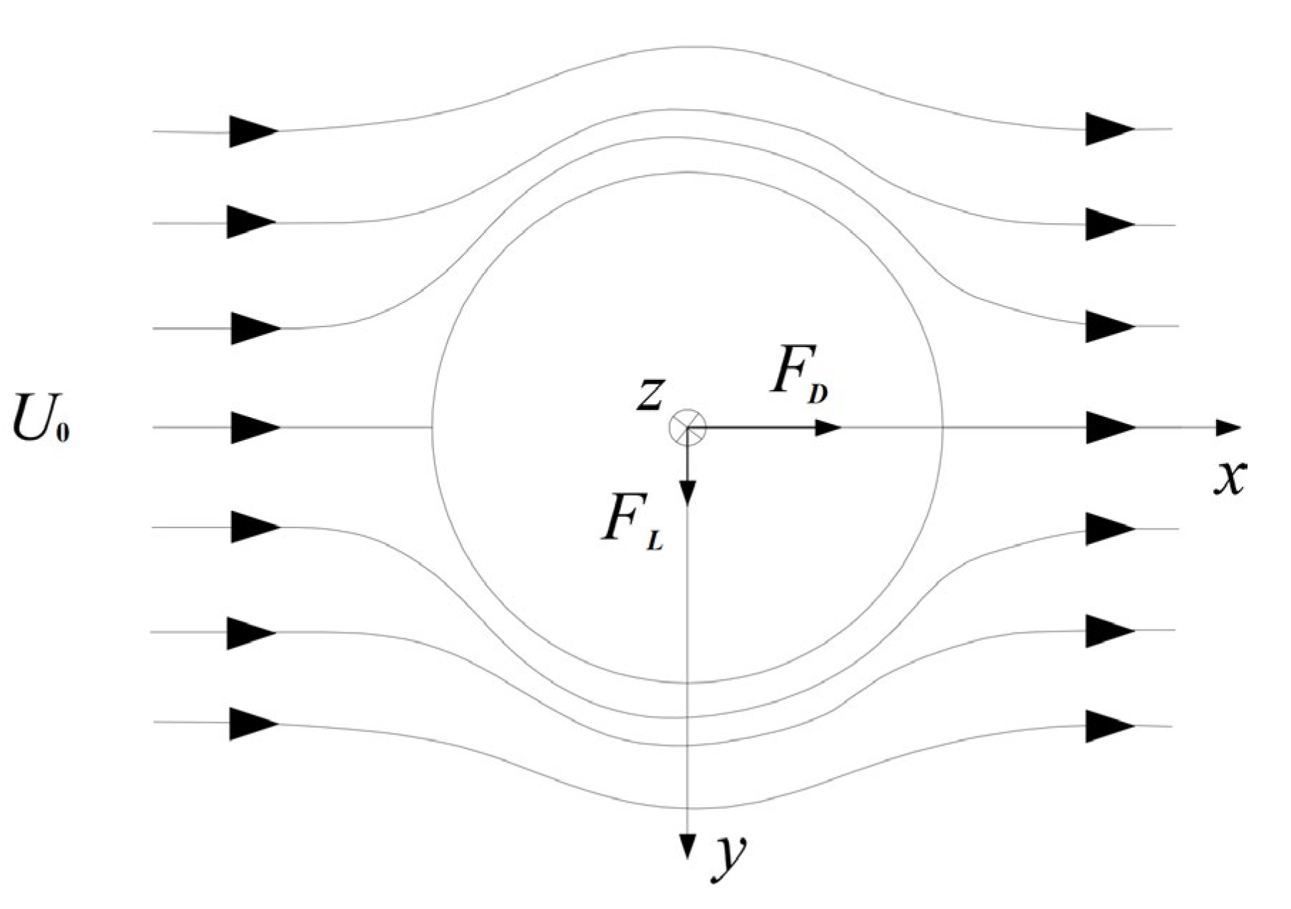
The experiment employs a three-component force balance to directly measure the time-averaged drag FD (and, when desired, the lift FL); the mechanical layout and sensor coordinate system are illustrated in Figure 7. Leveraging real-time data acquisition, drag is recorded across a series of Reynolds numbers and benchmarked against canonical empirical circular-cylinder datasets to enhance measurement fidelity. At low Re, departures of the measured FD from classical correlations are attributable chiefly to end effects, wall (confinement) interference, and uncertainty in free-stream velocity determination—offering a prototypical case study for students to dissect error sources.

3.3. AI and Data-Driven Modeling Approach

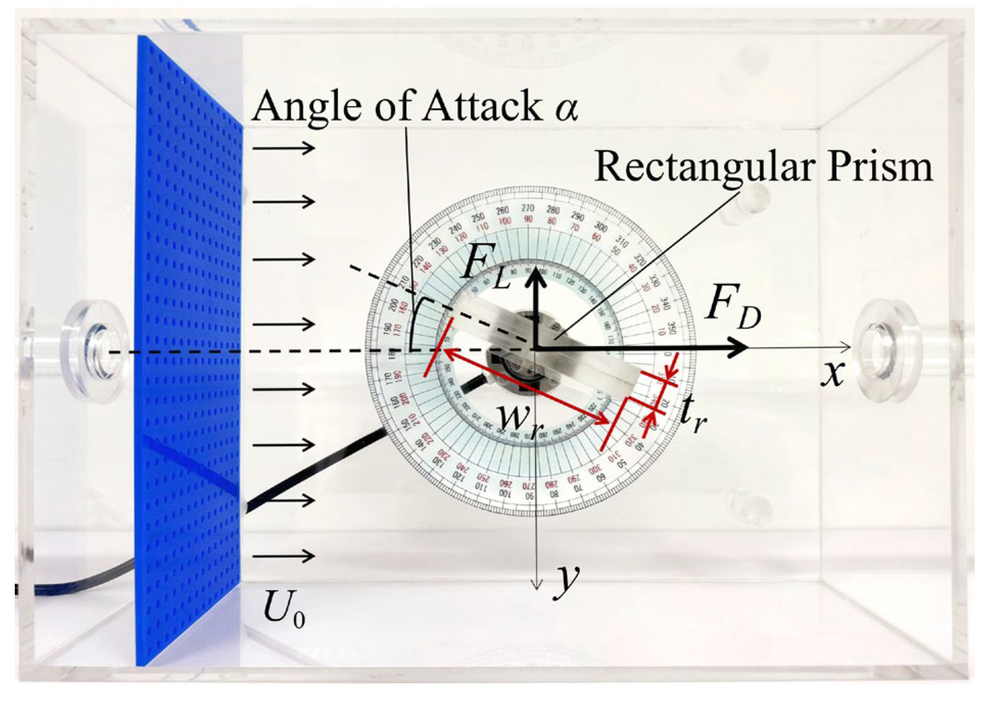
For non-circular or geometrically intricate bluff bodies, conventional analytical or semi-empirical formulations struggle to reconcile predictive accuracy with the need for rapid evaluation. To deepen exploitation of the experimental platform’s data and to reinforce the inquiry-driven (research) dimension of instruction, we incorporate an artificial neural network (ANN) to regress the drag and lift coefficients of a finite-thickness rectangular bluff body. This establishes a transferable, student-oriented paradigm for data-driven modeling. A finite-thickness rectangular cylinder with width wr = 7 cm, thickness tr = 2 cm, and height hr = 12 cm is employed as the illustrative test article, and its arrangement within the measurement tank is shown in Figure 8.
During the experiments, the freestream velocity U0, angle of attack α, and immersion depth H (kept below the cylinder height to mitigate free-surface interference) were varied under a strict one-factor-at-a-time protocol: in any given run, only one of these parameters (velocity, angle of attack, or immersion ratio) was changed, while the remaining parameters were held stable within approximately 1% to minimize passive coupling and confounding effects. A force measurement system was used to synchronously acquire drag and lift, enabling analysis of the influence of flow velocity, angle of attack, and immersion depth on the wake characteristics. After extraction of statistically steady segments, temporal averaging, and outlier rejection, an artificial neural network (ANN) dataset was constructed. To reduce computational cost, a single random hold-out partition was performed, splitting the data into mutually independent training, validation, and test sets in proportions of 70%, 15%, and 15%, respectively. The training set was used solely for parameter (weight) optimization; the validation set was used only for hyperparameter selection and early stopping; and the test set was invoked exactly once after all model architecture and hyperparameters had been definitively fixed, without participating in any tuning procedure.
To neutralize disparities in physical units and scale, the ANN ingests a three-component, dimensionless feature vector composed of the Reynolds number, angle of attack, and normalized submergence depth:
X = [ x 1 , x 2 , x 3 ] T = [ R e ,   α * , H *   ] T
The Reynolds number Re is defined using the prism (rectangular column) thickness tt as the characteristic length, Re = U0t/ν. Constrained by the test facility’s maximum flow rate, Re is swept from 50 to 500 in increments of 50. The normalized angle of attack is α* = α/(π/2), with the physical angle αα varying from 0° to 90° in 3° steps. The dimensionless submergence is H* = H/t, with H ranging from 5 cm to 11 cm in 1 cm increments. The network outputs the nondimensional drag and lift coefficients, assembled into a two-component output vector:
Y = [ y 1 , y 2 ] T = [ C D ,   C L ] T
To improve training efficiency and stability while mitigating adverse effects arising from disparate parameter scales, all input and output variables are min–max scaled before model training so that each is mapped to the interval (−1, 1). The scaling transformation [24] is given by the following expression:
i n = ( i n ,   max i n ,   min ) ( i i min ) ( i max i min ) + i n ,   min
Let i denote any input feature with extrema imin and imax; its scaled counterpart is in, which by construction satisfies in,min = −1 and in,max = 1. The inverse scaling is also applied to the model outputs to recover their physical (dimensioned or conventionally nondimensional) values. Specifically,
o = ( o n o n ,   min ) ( o max o min ) ( o n ,   max o n ,   min ) + o min
Here, o denotes the (physical) output variable with bounds omin and omax; its normalized counterpart on is constrained by construction to the interval −1, 1, i.e., on,min = −1 and on,max = 1.
The artificial neural network is configured as a fully connected, single-hidden-layer feedforward model. The input layer includes 3 nodes; the hidden layer contains k neurons, where k is subsequently selected based on convergence diagnostics; and the output layer comprises 2 nodes. The hidden layer utilizes the rectified linear unit (ReLU) activation function.
ReLU ( x ) = max ( 0 ,   x )
The derivative employed during backpropagation is:
ReLU ( x ) = 0 , x < 0 1   , x > 0
At x = 0, an admissible subgradient may be chosen as 0 or 1 (we adopt a conventional selection when needed). A single-hidden-layer fully connected feedforward network with ReLU activation enjoys the universal approximation property once the hidden width is sufficiently large. A linear (identity) activation f(x) = x is used at the output layer. Hence, the single-hidden-layer network is expressed as:
h 1 h 2 h k = w h 11 w h 12 w h 13 w h 21 w h 22 w h 23 w h k 1 w h k 2 w h k 3   x 1 n x 2 n x 3 n +   b h 1 b h 2 b h k
y 1 n y 1 n = w y 11 w y 12 w y 1 k w y 21 w y 22 w y 2 k ReLU ( h 1 ) ReLU ( h 2 ) ReLU ( h k ) + b y 1 b y 2
where x1n, x2n, and x3n denote the input-layer neurons corresponding to the normalized input parameter values. hk denotes a neuron in the hidden layer. wh denotes the weights connecting the input layer to the hidden layer; for example, whk3 is the weight between the third input neuron and the k-th hidden neuron. bh denotes the bias associated with a hidden-layer neuron. y1n and y2n denote the output-layer neurons corresponding to the normalized output parameter values. wy denotes the weights connecting the hidden layer to the output layer; for example, wy2k is the weight between the k-th hidden neuron and the second output neuron. by denotes the bias associated with an output-layer neuron. The hidden-layer width together with these weights and biases constitutes the trainable parameters used to build the predictive model.

4. Results

4.1. Surface Pressure Distribution

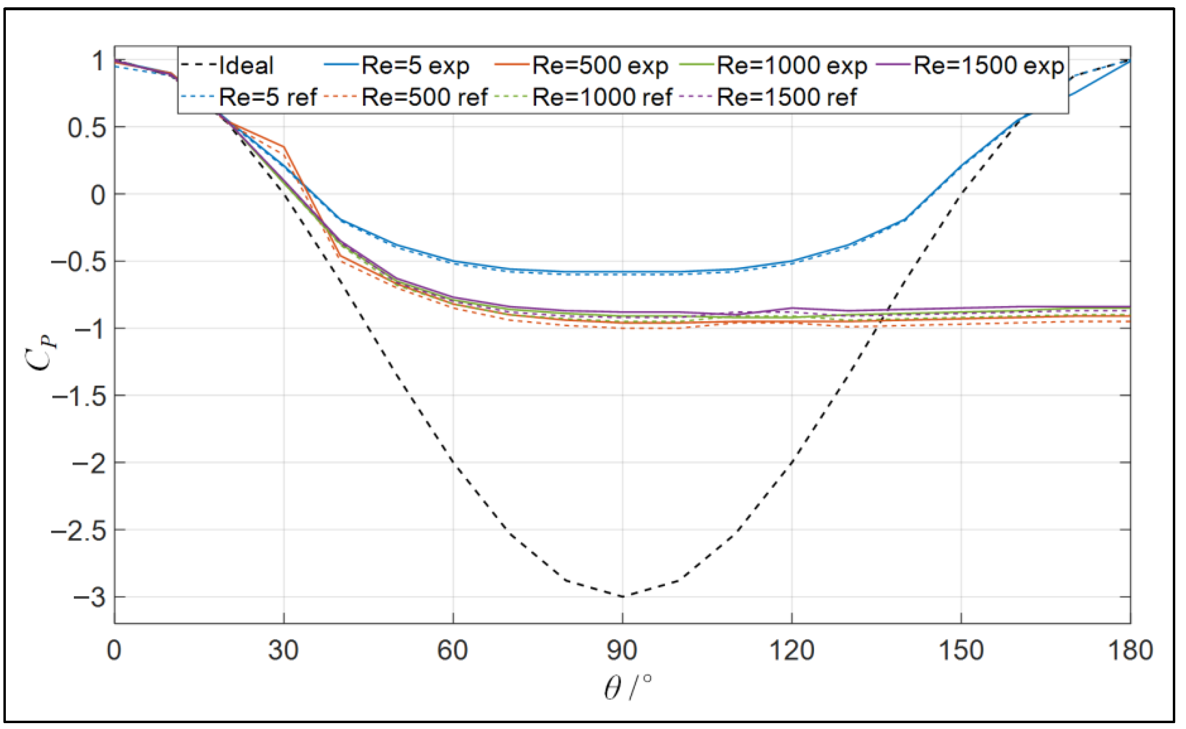
Surface pressure distributions were measured, at ambient temperature, on a stationary, non-rotating circular cylinder whose axis is perpendicular to the incoming flow. At a selected cross-section, multiple pressure taps were installed circumferentially. By rotating the cylinder, each tap was brought successively to prescribed azimuthal (polar) positions, enabling acquisition of the pressure coefficient under several inflow conditions at a water submergence depth of 10 cm. Based on the facility’s flow-rate limits, the Reynolds number was maintained within 5–1500, and four representative operating conditions, Re = 5, 500, 1000, and 1500, were chosen. Measurement points span the angular interval from 0° (defined at the upstream stagnation point) along one side of the cylinder surface to 180° (trailing edge). The experimental data are compared against the ideal inviscid potential-flow solution and selected empirical/semi-empirical reference distributions, as presented in Figure 9.
Comparison with the ideal potential-flow analytical solution and reference empirical (semi-empirical) curves shows that the upstream stagnation-point deviation is only about 1%. As θ increases through 10–40°, the surface pressure drops rapidly into suction; an inflection then emerges near 70–80°, establishing a broad plateau CP = −0.9 ∼−1.0, far higher (smaller in absolute magnitude) than the ideal prediction CP = −3 at 90°. This reflects early separation of a laminar (or transitional) boundary layer and dominance of base (wake) pressure. The inferred separation angle (≈70–80°) is modestly downstream of classical low-Re smooth-cylinder values, plausibly influenced by end- and support-induced three-dimensional disturbances, local momentum redistribution, and finite-length effects. Minimal variation in the amplitude or shape of the negative-pressure plateau across Re = 500–1500 indicates that the flow in this low-to-moderate Re range has not yet transitioned to turbulent reattachment or entered a “drag crisis” mechanism. Agreement between experimental and reference curves is good over the mid and rear sectors, while slight discrepancies in the early acceleration region gradients likely arise from (i) embedded assumptions regarding boundary-layer momentum deficit in the empirical formulations, (ii) angular positioning and dynamic-pressure calibration uncertainties (on the order of a few percent), and (iii) spatial smoothing of local static pressure by the tap diameter. Collectively, the results elucidate how viscosity, separation, and wake dynamics break the symmetry of ideal potential flow and quantitatively delineate the gap between the theoretical upper bound and the realized flow field.

4.2. Drag Measurement

To assess the reliability and repeatability of the setup, steady hydrodynamic tests were conducted on a cylinder (immersion depth 11 cm) under constant free-stream conditions across the subcritical Reynolds number range Re = 200–1400, with multiple repeated runs. Calibrated force sensors resolved the streamwise (drag) and vertical (lift) components; because the measured lift was zero, the analysis focuses solely on drag. The resulting drag data are compared with values derived from the literature [1,5] in Table 1.
As summarized in Table 1, comparison with canonical smooth-cylinder reference data shows that the relative drag deviations span −10.25% to +7.91%, with a mean signed deviation of +2.05%, a mean absolute deviation of 6.43%, and a root-mean-square (RMS) percentage deviation of 6.87%. These metrics demonstrate good accuracy and repeatability of the force measurement system. At Re = 200, the drag magnitude falls to the 10−5 N order; constrained by the system signal-to-noise ratio and force resolution, the relative contributions of residual baseline (offset) and zero drift become amplified, producing the largest negative deviation. The slight positive deviations at intermediate to higher Re likely reflect the combined influence of modest test-section blockage, three-dimensional end and free-surface leakage, free-stream turbulence intensity, and minor surface roughness. The alternation of positive and negative deviations without monotonic drift further supports the robustness of the calibration factor and processing chain. Physically, the data recover the classical subcritical trend of a gradual decrease in cylinder drag coefficient with increasing Re (even though the CD curve is not explicitly shown), furnishing a reliable baseline for later implementation of flow-control strategies or extension to higher Re, while underscoring the need to quantify more precisely the uncertainty contributions from blockage ratio, turbulence intensity, and water temperature (viscosity).

4.3. Development and Performance Evaluation of the Predictive Model

To develop an artificial neural network (ANN) predictor that strikes an effective balance between accuracy and parsimony, we adopted a structural optimization strategy of progressing from simple to more complex configurations and then pruning by preferential simplification. A parameter sweep was conducted on the number of neurons in the single hidden layer. Guided by the empirical guideline in the literature [25]—namely that the hidden layer size should be approximately 1.5–3 times the number of input neurons—and accounting for the dataset’s sample size and feature dimensionality, we selected the range 5–12 as candidate architectures. Each candidate was independently trained and validated in MATLAB R2024a; convergence rate and training/validation errors were compiled (Table 2), and evidence of overfitting (suppressed training error accompanied by a validation error rebound) or underfitting (uniformly large errors with further gains still achievable by adding neurons) was assessed. The architecture with nine hidden neurons delivered the best composite performance, thereby fixing the hidden-layer size at k = 9.
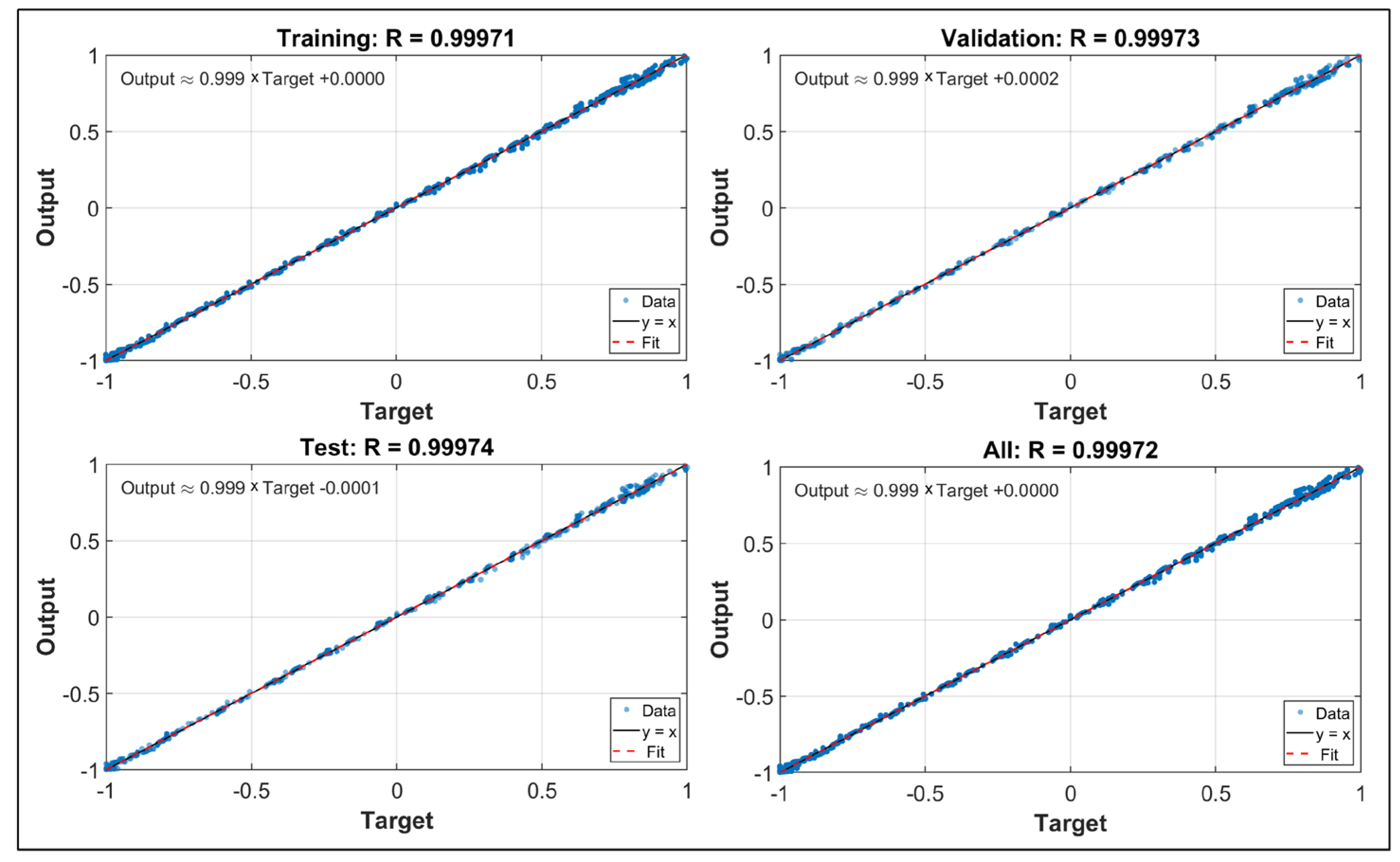
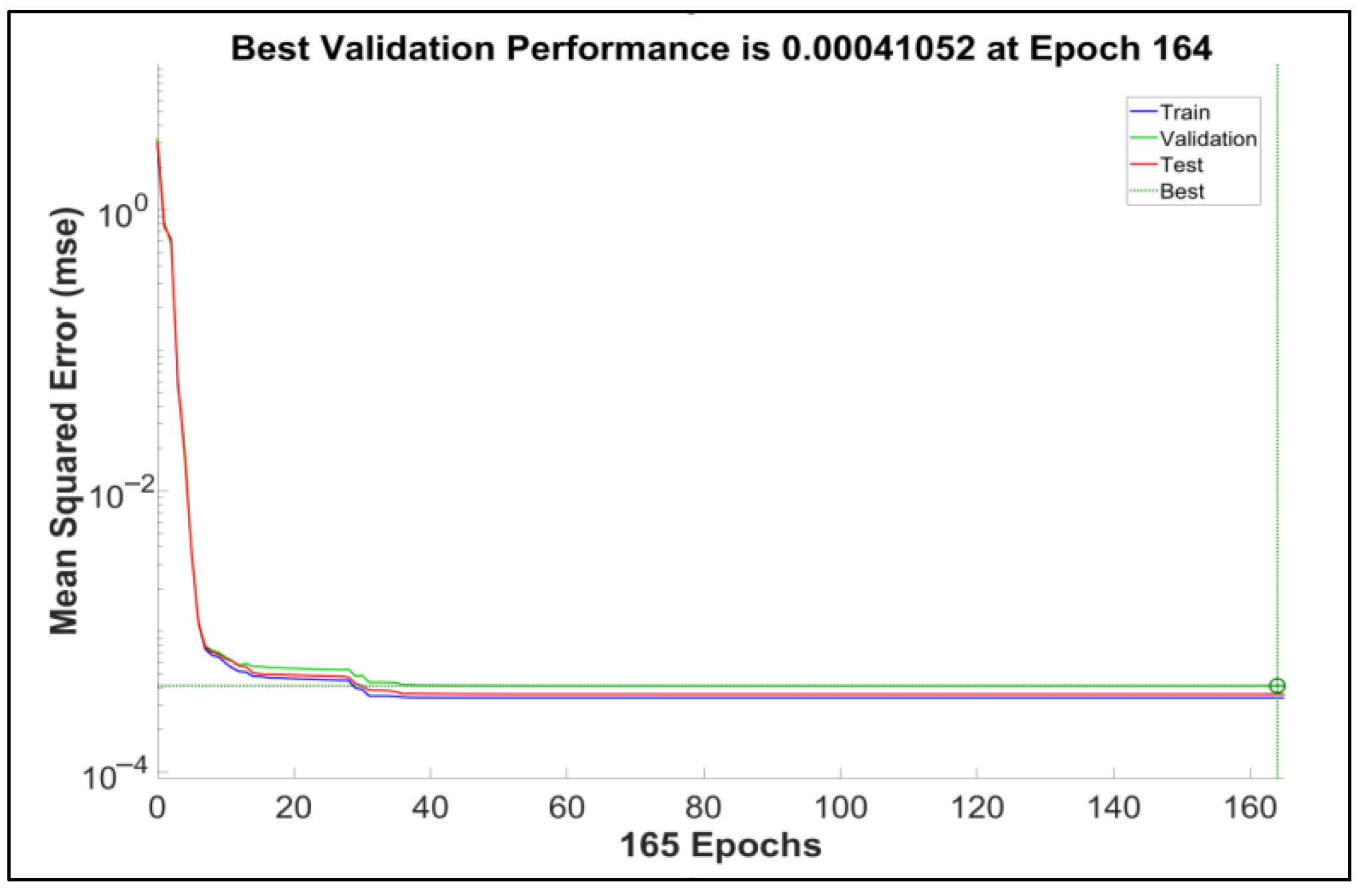
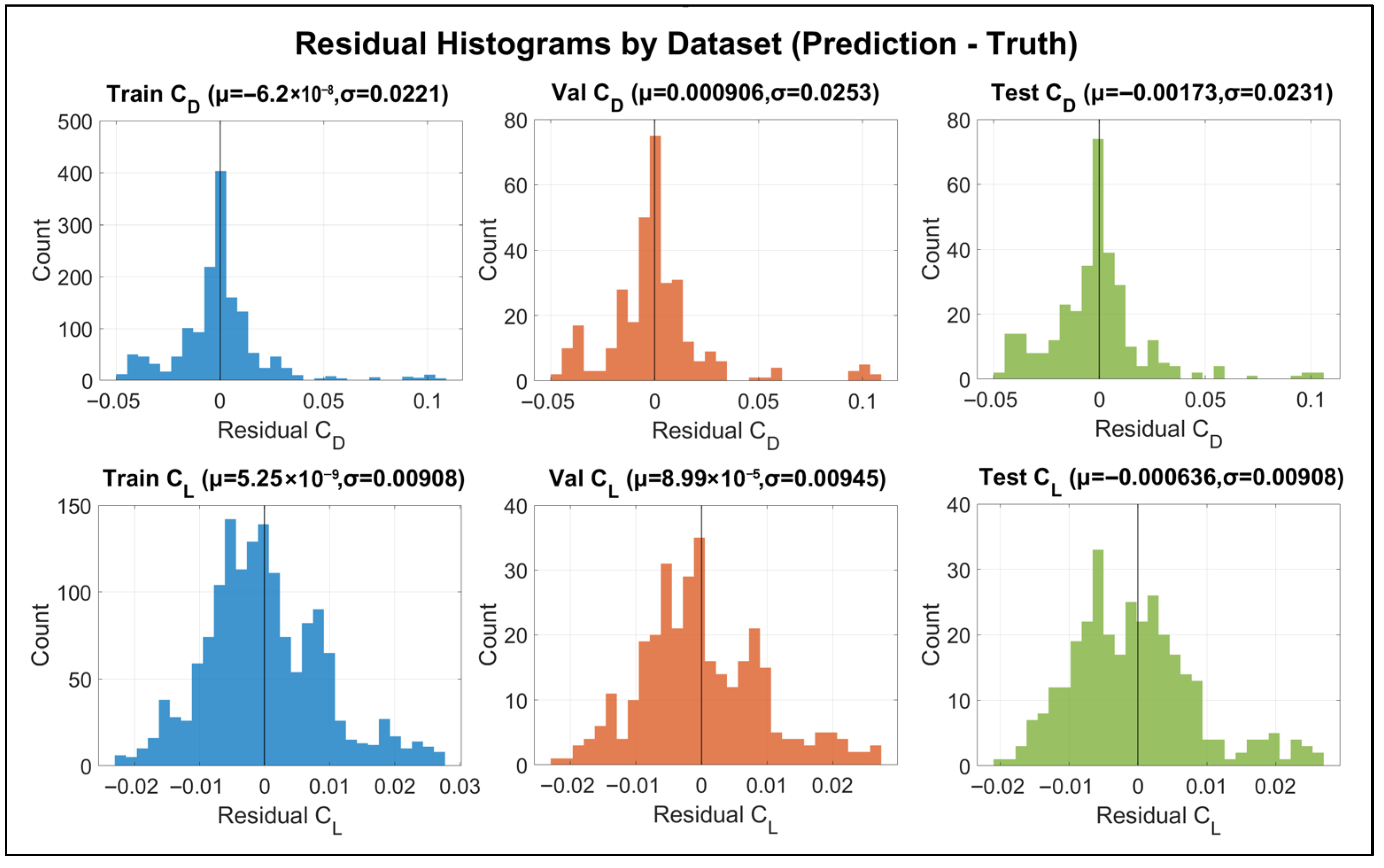
Figure 10, Figure 11 and Figure 12 present the regression plot and the mean squared error (MSE) validation trajectory for the model employing 9 neurons in its single hidden layer. Figure 10 shows that the predicted versus target values form a tight cluster about the ideal 1:1 line; the fitted line exhibits a slope near unity and an intercept approaching zero, with correlation coefficients for all subsets exceeding 0.99, evidencing excellent predictive fidelity. In Figure 11, the MSE for each data subset undergoes a rapid initial decline and reaches a plateau after roughly 164 iterations, ultimately converging to a low value (MSE = 0.00041502), corroborating the model’s stability and robustness. Figure 12 further demonstrates that the residual means for CD and CL across the training, validation, and test sets are on the order of 10−3 or smaller (CD: μ between −1.73 × 10⁻³ and 9.06 × 10⁻⁴; CL: μ between −6.36 × 10⁻⁴ and 8.99 × 10⁻⁵), which—when compared with their respective standard deviations (CD: σ ≈ 0.022–0.025; CL: σ ≈ 0.0090–0.0095)—indicates the absence of systematic bias. The σ values for all three data partitions reveal no overfitting; residual distributions are approximately unimodal and symmetric, and CL exhibits lower dispersion than CD, collectively attesting to the model’s strong generalization capacity and statistical robustness.
In the trained ANN architecture, the input-to-hidden layer weight matrix has dimensions 9 × 3, while the hidden-to-output layer weight matrix is 2 × 9. The hidden layer bias term is represented by a 9 × 1 matrix, and the output layer bias by a 2 × 1 vector. Following training and performance assessment, these weights and biases were extracted to formulate predictive expressions. Thus, the hidden layer net input (linear combination) is given in Equation (14), and the normalized output variables are defined in Equation (15).
h 1 h 2 h 3 h 4 h 5 h 6 h 7 h 8 h 9 = 1.3460 0.1823 0.0038 0.0096 0.6000 0.0004 0.0066 1.2978 0.0012 0.0129 0.9694 0.0008 0.0383 1.0545 0.0002 0.0069 1.3853 0.0005 0.0329 0.0015 0.0004 1.2245 1.2621 0.0000 0.0287 1.5857 0.0013   x 1 n x 2 n x 3 n + 0.8186 0.2606 0.6677 0.4290 0.7516 0.1694 0.0156 0.0376 0.2618
y 1 n y 2 n = 0.1931 0.3217 0.6799 0.6035 0.5694 0.0789 1.1663 0.0021 0.1048 0.0189 2.4230 1.0777 0.4720 0.5828 1.1286 1.2368 0.0653 0.7589   ReLU ( h 1 ) ReLU ( h 2 ) ReLU ( h 3 ) ReLU ( h 4 ) ReLU ( h 5 ) ReLU ( h 6 ) ReLU ( h 7 ) ReLU ( h 8 ) ReLU ( h 9 ) + 0.7393 1.4682
In Equation (15), the hidden-layer activation function ReLU(hx) is evaluated as specified in Equation (10). The quantities y1n and y2n denote the model’s normalized outputs; applying the denormalization procedure defined in Equation (9) yields the drag coefficient CD and the lift coefficient CL.
Within the discrete parameter space Re = 50–500, α = 0–90°, and H = 5–11 cm, a stratified balanced sampling strategy was implemented: for each Reynolds number, three representative angles of attack (low/medium/high) were selected, and for every angle-of-attack combination, the immersion depths were uniformly allocated, yielding 30 representative operating conditions. The drag and lift coefficients CD and CL predicted by the present correlation were compared with estimates derived from the empirical formulas reported in Anderson’s monograph [26] (see Table 3). The two sets of results exhibit strong agreement in both the principal trends with respect to Re and α and in relative magnitudes, thereby supporting the applicability of the proposed modeling approach within the current parameter domain. The mean absolute deviation of CD is 3.122%, with a maximum of 6.596%; the mean absolute deviation of CL is 4.301%, with a maximum of 6.383%. All deviations are positive (predictions exceeding empirical estimates) and show no monotonic accumulation with Re, α, or H. This indicates that the positive bias reflects a mild systematic increment rather than a progressive drift, plausibly attributable to blockage effects associated with the finite test section. The few larger deviations occur primarily at intermediate Re where the drag coefficient is comparatively low, a behavior likely linked to transition sensitivity and signal-to-noise ratio limitations rather than to a structural deficiency of the model.

4.4. Sources of Uncertainty and Limitations

The results of this study are subject to additional uncertainties arising primarily from blockage effects, incoming-flow turbulence intensity, and viscosity drift due to water temperature variation. For the rectangular cylinder, the projected width in the flow direction varies with the angle of attack between its thickness tr and its width wr, yielding a geometric blockage ratio lying within the interval expressed in Equation (16):
β w = [ t r / w 0 ,   w r / w 0 ] = [ 0.04 ,   0.14 ]
Accounting for the open free surface and end leakage, an effective attenuation coefficient η ≈ 0.35 is adopted, leading to an effective blockage ratio given by Equation (17):
β eff = η β w = [ 0.014 ,   0.049 ] < 0.05
Within this low-blockage regime, a first-order wall-interference approximation is employed, as indicated in Equation (18):
Δ C D / C D k D β eff , Δ C L / C L k L β eff
Here, ΔCD and ΔCL denote the changes in the drag and lift coefficients induced by blockage; kD ≈ 1.2 and kL ≈ 0.8, the uncorrected drag coefficient is estimated to exhibit a positive bias of approximately 1.7–5.9%, while the uncorrected lift coefficient shows a positive bias of approximately 1.1–3.9%.
Although the incoming-flow turbulence intensity was not measured directly, it is empirically estimated as I ≈ 2% (consistent with the typical 1–3% range under flow-straightening plate conditions). This contributes an additional uncertainty of about 1% to the mean subcritical values of CD and CL. The laboratory water temperature was approximately 20 °C with a deviation of ±0.5 °C, corresponding to a kinematic viscosity ν ≈ 1.00 × 10⁻⁶ m2/s. The viscosity variation induced by temperature fluctuations is about 1%, yielding a similar 1% deviation in the Reynolds number Re; the propagated uncertainty transferred to CD and CL is <0.1% and therefore negligible. The principal limitation of this study is that the uncertainty analysis for the rectangular cylinder flow experiments relies on approximate methods and lacks rigorous, high-fidelity quantification. Future work will focus on a more precise evaluation of blockage effects and direct, high-accuracy measurement of the incoming turbulence intensity.

5. Discussion

Across the investigated low-to-moderate Reynolds number regime, the instructional bluff-body flow platform developed herein enabled synchronous acquisition of multi-point surface pressure distributions and integral hydrodynamic forces on the cylinder. The circumferential pressure evolution—elevated at the forward stagnation point, a rapid downstream decline, then a gradual variation near the separation angle—matches canonical subcritical behavior reported in the literature, with no drag-crisis-associated abrupt reduction, evidencing that flow management and flume scaling effectively suppressed sidewall and free-surface perturbations to mainstream uniformity. Drag trends measured by the three-component force sensor are consistent with published data, and the scatter exhibits no systematic drift, corroborating structural stiffness and calibration stability. Incorporation of an artificial neural network (ANN) for predicting the drag and lift of flow past a rectangular cylinder preserved strong evaluative performance, indicating that principal dependencies can be reconstructed from a constrained feature set (Reynolds number, angle of attack, and submergence depth); residual errors predominantly stem from the transient vortex-shedding phase and end effects not explicitly parameterized. Pedagogical deployment showed that students, by traversing the sequence “local pressure → global force → data-driven modeling,” achieved cross-stage cognitive transfer from physical mechanism understanding to intelligent prediction, more effectively stimulating inquiry and reflective thinking than conventional single-purpose verification experiments.
The proposed low-cost instructional platform exhibits reliability and pedagogical value; nevertheless, its performance envelope and breadth of application remain constrained by scientific and technical limitations. Principal constraints include: pump capacity and flume geometry, which cap the upper Reynolds number and currently preclude access to the critical and supercritical flow regimes; the adoption at this stage of a mid-span quasi-two-dimensional assumption without quantitative characterization of finite-height cylinder end effects and free-surface-induced three-dimensionality; an uncertainty analysis that relies on approximate methods and lacks rigorous quantification, including direct measurement of turbulence intensity; potential attenuation of three-dimensional vortex coherence caused by the combined influence of a free surface and open-ended boundaries, thereby modulating lift fluctuations; an insufficient sensor signal-to-noise ratio at low force levels, limiting precise identification of the dominant lift frequency; and a comparatively narrow training dataset for the artificial neural network, whose generalization across varied body geometries and broader Reynolds number ranges is weakened by the absence of embedded physical constraints. Future work will expand the attainable Reynolds number range through increased flow capacity and geometric scaling; deploy end plates or cover plates to mitigate end effects and free-surface coupling; conduct quantitative evaluation of three-dimensional end effects and the validity bounds of the quasi-two-dimensional approximation; integrate high-density pressure scanning and flow-field visualization (e.g., PIV); incorporate physics-informed constraints or hybrid network architectures to enhance model interpretability; and establish a quantitative framework for assessing instructional effectiveness, thereby progressively strengthening the platform’s research and educational value.

6. Conclusions

This work develops a low-cost, reproducible instructional platform for bluff-body flow that unifies transparent flume multi-point surface pressure measurement, synchronous global hydrodynamic force acquisition, and ANN-enabled data-driven prediction. The measured circumferential pressure distribution around the cylinder aligns with canonical subcritical flow behavior; drag measurements exhibit stable performance with an average absolute deviation of approximately 6.43%. ANN predictions for CD and CL achieve low error levels, with test-set mean absolute relative errors near 4%, correlation coefficient R > 0.99, and residuals free of systematic bias. These outcomes confirm the platform’s dual capability: supporting core fluid mechanics theory verification while illustrating the efficacy of data-driven modeling for rapid flow-parameter estimation. The experimental results indicate that the platform enhances students’ integrated competencies across the full workflow of experimental design, data analysis, and intelligent modeling, demonstrating strong potential for practical application.
In sum, the findings substantiate that hydrodynamic instruction for representative marine engineering bluff bodies can, within economical constraints, realize coupled local–global data fusion and AI-enabled modeling, yielding a scalable, transferable intelligent experimental pathway. Future developments will target the following: broadening the accessible Re range and geometric repertoire; enhancing circumferential and temporal resolution to clarify separation and vortex-shedding dynamics; fusing multi-modal transient flow diagnostics; embedding physical constraints or hybrid intelligent architectures to elevate generalization and interpretability; and instituting systematic quantitative assessment of instructional impact. Advancing these fronts will position the platform for deeper translation into research validation and open innovation laboratories, fostering a sustainably evolving intelligent experimental ecosystem in fluid mechanics.

Author Contributions

Conceptualization, H.Z. and B.Z.; methodology, H.Z.; software, H.Z.; validation, B.Z., X.L. and Q.L.; formal analysis, H.Z.; investigation, H.Z.; resources, X.L.; data curation, H.Z.; writing—original draft preparation, H.Z.; writing—review and editing, H.Z.; visualization, H.Z.; supervision, H.Z.; project administration, H.Z.; funding acquisition, X.L. All authors have read and agreed to the published version of the manuscript.

Funding

This research was funded by the National Natural Science Foundation of China (Grant No. 52471301), the Experimental Technology Research Project of Zhejiang University (Grant No. SYBJS202310), and the 2025 Zhejiang University Undergraduate “X + AI” Experimental Teaching Reform Initiative.

Institutional Review Board Statement

Not applicable.

Informed Consent Statement

Not applicable.

Data Availability Statement

The study data are available within this article.

Conflicts of Interest

The authors declare no conflicts of interest.

References

  1. Zdravkovich, M.M. Flow Around Circular Cylinders. Vol. 1: Fundamentals; Oxford University Press: Oxford, UK, 1997. [Google Scholar]
  2. Williamson, C.H.K. Vortex dynamics in the cylinder wake. Annu. Rev. Fluid Mech. 1996, 28, 477–539. [Google Scholar] [CrossRef]
  3. Roshko, A. On the drag and shedding frequency of two-dimensional bluff bodies. NACA Rep. 1954, 1191. [Google Scholar]
  4. Bearman, P.W. Vortex shedding from oscillating bluff bodies. Annu. Rev. Fluid Mech. 1984, 16, 195–222. [Google Scholar] [CrossRef]
  5. Norberg, C. An experimental investigation of the flow around a circular cylinder: Influence of aspect ratio. J. Fluid Mech. 1994, 258, 287–316. [Google Scholar] [CrossRef]
  6. Schewe, G. On the force fluctuations acting on a circular cylinder in crossflow from subcritical up to transcritical Reynolds numbers. J. Fluid Mech. 1983, 133, 265–285. [Google Scholar] [CrossRef]
  7. Sánchez Martín, J.; Vázquez Rodríguez, S.; García Cubero, M.T. FLUID-LABVIR: A hybrid virtual laboratory platform for fluid mechanics engineering education. Educ. Chem. Eng. 2021, 36, 123–134. [Google Scholar]
  8. Freeman, S.; Eddy, S.L.; McDonough, M.; Smith, M.K.; Okoroafor, N.; Jordt, H.; Wenderoth, M.P. Active learning increases student performance in science, engineering, and mathematics. Proc. Natl. Acad. Sci. USA 2014, 111, 8410–8415. [Google Scholar] [CrossRef]
  9. Prince, M. Does active learning work? A review of the research. J. Eng. Educ. 2004, 93, 223–231. [Google Scholar] [CrossRef]
  10. Lu, G.D.; Li, T.Y. Reflections on Pathways for the Construction and Development of Emerging Engineering Education. Res. High. Eng. Educ. 2017, 3, 20–26. [Google Scholar]
  11. Zhong, D.H. Connotations and Action Framework for Building Emerging Engineering Education. Res. High. Eng. Educ. 2017, 3, 1–6. [Google Scholar]
  12. Rowley, C.W.; Dawson, S.T.M. Model reduction for flow analysis and control. Annu. Rev. Fluid Mech. 2017, 49, 387–417. [Google Scholar] [CrossRef]
  13. Duraisamy, K.; Iaccarino, G.; Xiao, H. Turbulence modeling in the age of data. Annu. Rev. Fluid Mech. 2019, 51, 357–377. [Google Scholar] [CrossRef]
  14. Brunton, S.L.; Noack, B.R.; Koumoutsakos, P. Machine learning for fluid mechanics. Annu. Rev. Fluid Mech. 2020, 52, 477–508. [Google Scholar] [CrossRef]
  15. Ling, J.; Kurzawski, A.; Templeton, J. Reynolds stress modeling using deep neural networks with embedded invariance. J. Fluid Mech. 2016, 807, 155–166. [Google Scholar] [CrossRef]
  16. Wang, J.-X.; Wu, J.-L.; Xiao, H. Physics-informed machine learning approach for reconstructing Reynolds stress modeling discrepancy. Phys. Rev. Fluids 2017, 2, 034603. [Google Scholar] [CrossRef]
  17. Raissi, M.; Perdikaris, P.; Karniadakis, G.E. Physics-informed neural networks: A deep learning framework for solving forward and inverse problems. J. Comput. Phys. 2019, 378, 686–707. [Google Scholar] [CrossRef]
  18. Fukami, K.; Fukagata, K.; Taira, K. Super-resolution reconstruction of turbulent flows with machine learning. J. Fluid Mech. 2019, 870, 106–120. [Google Scholar] [CrossRef]
  19. Guo, X.; Li, W.; Iorio, F. Convolutional neural networks for steady flow approximation. In Proceedings of the 22nd ACM SIGKDD International Conference on Knowledge Discovery and Data Mining (KDD’16), San Francisco, CA, USA, 13–17 August 2016; ACM: New York, NY, USA, 2016; pp. 481–490. [Google Scholar] [CrossRef]
  20. Milano, M.; Koumoutsakos, P. Neural network modeling for near wall turbulent flow. J. Comput. Phys. 2002, 182, 1–26. [Google Scholar] [CrossRef]
  21. Han, Y.; Wang, Y.; Guo, C.Y.; Wang, C.; Sun, C. Experimental teaching platform for an oscillating rotating cylinder based on the Magnus effect. Exp. Technol. Manag. 2020, 37, 54–57. [Google Scholar] [CrossRef]
  22. Guo, C.Y.; Zhang, H.R.; Han, Y.; Kuai, Y.F.; Li, R.X.; Gao, Y. Design of a high-fidelity flow field measurement experimental teaching platform based on SPIV technology. Mech. Pract. 2025, 47, 416–425. [Google Scholar]
  23. Vinuesa, R.; Brunton, S.L.; McKeon, B.J. The transformative potential of machine learning for experiments in fluid mechanics. Nat. Rev. Phys. 2023, 5, 536–545. [Google Scholar] [CrossRef]
  24. Vijaya Kumar, S.D.; Lo, M.; Karuppanan, S.; Ovinis, M. Empirical failure pressure prediction equations for pipelines with longitudinal interacting corrosion defects based on artificial neural network. J. Mar. Sci. Eng. 2022, 10, 764. [Google Scholar] [CrossRef]
  25. González-Díaz, R.; Gutiérrez-Naranjo, A.M.; Paluzo-Hidalgo, E. Two-hidden-layer feedforward neural networks are universal approximators: A constructive approach. arXiv 2019, arXiv:1907.11457. Available online: https://arxiv.org/abs/1907.11457 (accessed on 14 August 2025).
  26. Anderson, J.D. Fundamentals of Aerodynamics, 6th ed.; McGraw-Hill Education: New York, NY, USA, 2017. [Google Scholar]
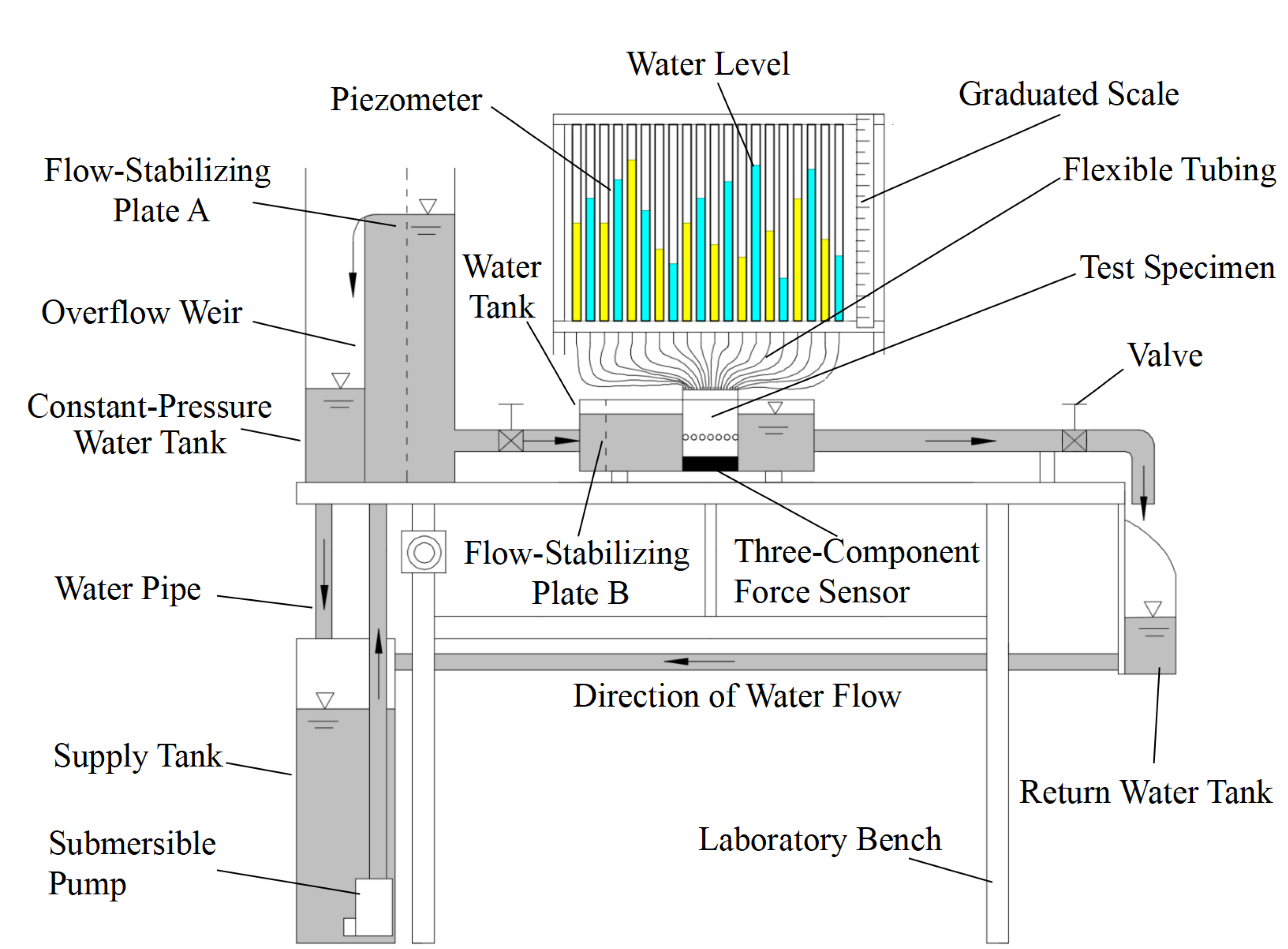
Figure 1. Schematic of the experimental apparatus.
Jmse 13 01761 g001
Figure 2. Measuring flume.
Jmse 13 01761 g002
Figure 3. Cylinder and multi-point pressure measurement device.
Jmse 13 01761 g003
Figure 4. Force measurement system.
Jmse 13 01761 g004
Figure 5. Overall photograph of the integrated pressure and force measurement apparatus.
Jmse 13 01761 g005
Figure 6. Schematic of pressure tap locations on the circular cylinder in crossflow.
Jmse 13 01761 g006
Figure 7. Schematic of drag/lift and the sensor coordinate system.
Jmse 13 01761 g007
Figure 8. Arrangement of the rectangular cylinder.
Jmse 13 01761 g008
Figure 9. Comparison of pressure coefficient distributions.
Jmse 13 01761 g009
Figure 10. Regression plot of the model.
Jmse 13 01761 g010
Figure 11. Performance validation curve of the model.
Jmse 13 01761 g011
Figure 12. Histograms of residuals for CD and CL.
Jmse 13 01761 g012
Table 1. Comparison of measured crossflow drag results.
ReFD/NDeviation/%
ReferenceTest
2002.83 × 10−52.54 × 10⁻⁵−10.25
4001.11 × 10−41.19 × 10⁻⁴+7.21
6002.46 × 10−42.56 × 10⁻⁴+4.07
8004.30 × 10−44.64 × 10⁻⁴+7.91
10006.60 × 10−46.41 × 10⁻⁴−2.88
12001.28 × 10−31.36 × 10⁻³+6.25
Table 2. Performance of single-hidden-layer ANN models with different numbers of hidden neurons.
IndexHidden NeuronsR2
150.9623
260.9654
370.9712
480.9827
590.9997
6100.9977
7110.9934
8120.9931
Table 3. Back-testing results for drag and lift coefficients.
ReαH/cmCDDeviation/%CLDeviation/%
Exp.EquationExp.Equation
50660.1230.1262.4390.1970.2053.850
5045101.3041.331.9940.7990.8121.627
5072111.8952.026.5960.5640.5924.965
508792.2372.2580.9390.1180.1256.383
100350.0920.0986.5220.1330.1426.383
1003981.0921.1253.0220.6580.694.863
1007591.8921.921.4800.4040.4214.156
150960.1070.1135.6070.1790.1885.263
1505171.2921.3726.1920.8270.8664.691
15069111.8921.9050.6870.6250.6564.943
200380.0870.093.4480.1200.1232.227
20048101.2021.2786.3230.7990.8384.881
2008462.0522.144.2880.3570.3744.703
250670.1070.1091.8690.1960.2044.337
2506951.8831.8860.1590.6310.6614.798
300350.0810.0832.4690.0990.1034.357
300680.1070.1080.9350.1960.2044.337
3006661.7991.8010.1110.7240.7351.547
3505771.5191.5371.1850.9210.9230.195
35072101.9411.9530.6180.5520.5856.021
400670.0920.0986.5220.1960.2044.337
4003690.9921.044.8390.6390.6714.975
40063111.6921.7181.5370.7050.7425.248
4008781.9922.031.9080.1390.1432.789
45012100.1520.1551.9740.2350.2454.255
4504291.0021.0676.4870.7330.7725.292
45066101.7021.7623.5250.6960.7315.089
45078111.8921.984.6510.3850.4014.048
50066111.7331.7752.4240.6970.7335.093
5007851.9922.052.9120.4000.4143.386
Disclaimer/Publisher’s Note: The statements, opinions and data contained in all publications are solely those of the individual author(s) and contributor(s) and not of MDPI and/or the editor(s). MDPI and/or the editor(s) disclaim responsibility for any injury to people or property resulting from any ideas, methods, instructions or products referred to in the content.