A Nonlinear Filter Based on Fast Unscented Transformation with Lie Group State Representation for SINS/DVL Integration

Abstract

This study addresses the nonlinear estimation problem in the strapdown inertial navigation system (SINS) and Doppler velocity log (DVL) integrated navigation by proposing an improved filtering algorithm based on $S{E}_2(3)$ Lie group state representation. A dynamic model satisfying the group affine condition is established to systematically construct both left-invariant and right-invariant error state spaces, upon which two nonlinear filtering approaches are developed. Although the fast unscented transformation method is not novel by itself, its first integration with the $S{E}_2(3)$ Lie group model for SINS/DVL integrated navigation represents a significant advancement. Experimental results demonstrate that under large misalignment angles, the proposed method achieves slightly lower attitude errors compared to linear approaches, while also reducing position estimation errors during dynamic maneuvers. The 12,000 s endurance test confirms the algorithm’s stable long-term performance. Compared with conventional unscented Kalman filter methods, the proposed approach not only reduces computation time by 90% but also achieves real-time processing capability on embedded platforms through optimized sampling strategies and hierarchical state propagation mechanisms. These innovations provide an underwater navigation solution that combines theoretical rigor with engineering practicality, effectively overcoming the computational efficiency and dynamic adaptability limitations of traditional nonlinear filtering methods.

1. Introduction

As a self-contained navigation system entirely independent of external signals, the strapdown inertial navigation system (SINS) has become a core solution for modern underwater vehicles and marine navigation due to its superior anti-jamming capability and stealth characteristics. The system continuously monitors the carrier’s angular velocity and linear acceleration variations in real-time through high-precision inertial measurement units (IMUs), executing autonomous navigation solutions based on Newtonian mechanical principles [1]. With operational frequencies typically reaching hundreds of Hertz, SINS effectively meets high-dynamic navigation requirements in complex underwater environments. Nevertheless, due to the inherent bias instability and scale factor error of the inertial sensor, the system solution results will continue to diverge over time. This error accumulation characteristic renders pure inertial navigation inadequate for long-endurance applications demanding high precision. Consequently, integrated navigation techniques have gained universal adoption in both academic research and engineering practice, employing periodic error correction through external observation inputs [2,3,4]. Among available aiding sources, Doppler velocity logs (DVLs) leveraging the Doppler effect emerge as the most effective solution, offering unique underwater operational compatibility and velocity measurement accuracy. DVLs precisely measure seabed-relative velocity components by transmitting acoustic waves and analyzing echo signals via Doppler shift principles. This measurement methodology remains unaffected by aquatic environmental factors and exhibits no time-dependent error accumulation, thereby forming an ideal complement to SINS [5,6,7].

1.1. Research Background and Key Challenges

The SINS/DVL integrated navigation system implementation comprises three functionally coupled core modules: the mechanization module performs real-time updates of carrier state parameters including attitude, velocity, and position through inertial navigation differential equations; the state estimation module designs optimal estimation algorithms based on discrete system models; the feedback correction module realizes closed-loop modification through error estimate injection into the solution process. Existing research methods bifurcate into direct and indirect categories based on state variable selection approaches [8]. The direct method uses navigation parameters as state variables. This approach requires handling nonlinear system models. In contrast, the indirect approach employs navigation errors as states. This maintains linear or weak nonlinear system properties. Such characteristics are advantageous for classical Kalman filter applications. Both methodologies present complementary trade-offs requiring balanced evaluation of system complexity, computational efficiency and estimation accuracy. More fundamentally, the integrated system’s state estimation represents a strongly nonlinear constrained optimization problem whose complexity stems principally from coupling interactions between state-space parameters. Significant progress has recently been achieved in navigation modeling via differential geometry theory, particularly through the invariant extended Kalman filter (IEKF) developed by Barrau and Bonnabel’s team [9,10,11,12,13,14,15,16]—a landmark contribution that constructs linearization-independent error quantities to fundamentally overcome inherent error accumulation limitations in traditional nonlinear filtering. Theoretical analyses confirm IEKF’s rigorous preservation of global consistency in unobservable subspaces [17], a feature critical for long-duration navigation stability that has been industrially validated in SAGEM’s commercial navigation products.

Recent investigations [18,19,20,21] have demonstrated that error models exhibit universal adaptability to arbitrary misalignment angles when formulated within a group-affine mechanization framework. However, achieving stable convergence under large misalignment conditions necessitates the simultaneous fulfillment of two critical requirements: the mechanization process must preserve group-affine properties while the observation model must satisfy specific invariance constraints. During initial alignment of SINS/DVL integrated systems, maintaining group-affine properties in the mechanization typically disrupts the measurement model’s invariant structure [21]. Conversely, preserving measurement model invariance often requires sacrificing the group-affine characteristics in mechanization. This fundamental incompatibility between theoretical requirements has substantially restricted the method’s real-world engineering implementation. For addressing nonlinear estimation challenges in high-precision navigation, the unscented Kalman filter (UKF) presents a potential resolution [22]. Distinct from conventional extended Kalman filter (EKF) methods, UKF circumvents error quantity construction by directly propagating and updating global states through sigma points, thereby fundamentally eliminating approximation errors induced by linearization. Nevertheless, practical implementation of UKF encounters two primary challenges: first, its computational complexity exhibits exponential growth with increasing state dimensions, making real-time performance difficult to achieve in resource-constrained embedded systems; second, the standard unscented transformation (UT) process requires propagation of numerous sigma points, resulting in substantial computational overhead.

1.2. Innovative Approach and Technical Contributions

To address this challenge, the present study innovatively employs the geometric properties of the $S{E}_2(3)$ group to construct a unified state-space framework. This Lie group structure comprehensively describes the carrier’s pose information, including position, velocity, and attitude, while its corresponding Lie algebra $s{e}_2(3)$ provides the mathematical foundation for local linear space representation [23,24,25,26,27]. The group-algebra transformation mechanism offers a concise yet rigorous mathematical tool for nonlinear estimation under large misalignment conditions, preserving the intrinsic characteristics of nonlinear systems while facilitating linearization approaches for filter implementation. To meet high-precision nonlinear estimation requirements, this study adopts a refined unscented Kalman filter scheme featuring two key technical innovations: first, the introduction of a fast unscented transformation (FUT) algorithm that substantially reduces computational complexity through specialized processing of sigma points; second, the optimization of sigma-point propagation strategy within the group-affine model framework, where only dominant points undergo complete nonlinear propagation while other sampling points receive linear approximation. This hierarchical approach effectively reconciles the accuracy–efficiency trade-off, endowing the algorithm with both high estimation precision and real-time computational capability. For engineering implementation, the study establishes a comprehensive theoretical framework and technical methodology: the system model strictly adheres to Earth coordinate transformation principles to guarantee group-affine conditions; the filter derivation employs a unified formal representation based on Lie group theory; and experimental validation systematically evaluates algorithm performance through lake trial data analysis. It is worth noting that the primary contribution lies not in the proposal of FUT itself, but in its tight integration with the earth-fixed frame and the group-affine SINS/DVL model to achieve real-time high-precision navigation under large misalignment angles.

1.3. Paper Organization Overview

The remainder of this paper is organized as follows: Section 2 introduces the group-affine compliant state model and its transformation relationships in Earth coordinates; Section 3 systematically elaborates the UKF and FUKF derivation processes and their implementation within group state space; Section 4 conducts comparative experiments using real lake test data, quantitatively assessing the proposed model’s navigation accuracy and robustness; Section 5 summarizes critical findings.

2. Preliminary Knowledge

This section presents the dynamics of SINS expressed in a group-affine-compliant group representation, as derived in prior work.

In the Earth-Centered Earth-Fixed (ECEF) frame, the SINS dynamics can be represented in matrix form as follows [28]:

$${\dot{\mathbf{C}}}_b^e={\mathbf{C}}_b^e\left({\mathsf{\omega }}_{ib}^b\times \right)-\left({\mathsf{\omega }}_{ie}^e\times \right){\mathbf{C}}_b^e,$$

(1)

$${\dot{\mathbf{v}}}_{ib}^e={\mathbf{C}}_b^e{\mathbf{f}}_b-\left({\mathsf{\omega }}_{ie}^e\times \right){\mathbf{v}}_{ib}^e+{\mathbf{G}}_{ib}^e,$$

(2)

$${\dot{\mathbf{r}}}_{ib}^e={\mathbf{v}}_{ib}^e-\left({\mathsf{\omega }}_{ie}^e\times \right){\mathbf{r}}_{ib}^e,$$

(3)

where e, i, and b denote the ECEF, inertial, and body frames, respectively; $\left(\cdot \times \right)$ represents the skew-symmetric operation; ${\mathbf{C}}_b^e$ is the direction cosine matrix from the body to the ECEF frame; ${\mathbf{v}}_{ib}^e$ and ${\mathbf{r}}_{ib}^e$ denote the projections of the body’s velocity and position relative to the inertial frame in the ECEF frame; ${\mathsf{\omega }}_{ib}^b$ is the angular velocity; ${\mathbf{f}}_b$ represents the specific force; ${\mathsf{\omega }}_{ie}^e$ is the Earth’s rotation rate in the ECEF frame; and ${\mathbf{g}}_{ib}^e$ is the gravity vector. The relationship between the traditional velocity ${\mathbf{v}}_{eb}^e$ and the proposed velocity vector ${\mathbf{v}}_{ib}^e$ is given by Equation (4).

$${\mathbf{v}}_{ib}^e={\mathbf{v}}_{eb}^e+({\omega }_{ie}^e\times )r_{ib}^e={\mathbf{v}}_{eb}^e+({\omega }_{ie}^e\times )r_{eb}^e,$$

(4)

The relationship between the gravity vector $g_{ib}^e$ and ${\mathbf{G}}_{ib}^e$ is given by Equation (5).

$${\mathbf{G}}_{ib}^e=g_{ib}^e+{({\omega }_{ie}^e\times )}^2{r}_{ib}^e=g_{ib}^e+{({\omega }_{ie}^e\times )}^2{r}_{eb}^e,$$

(5)

The gyroscope measurement model is expressed as Equation (6).

$${\omega }_{ib}^b={\tilde{\omega }}_{ib}^b-{\epsilon }^b-{\eta }_g^b,$$

(6)

$${\dot{\epsilon }}^b=0,$$

(7)

where ${\tilde{\omega }}_{ib}^b$ is the noise-corrupted gyroscope output, ${\epsilon }^b$ is the gyroscope bias, and ${\eta }_g^b$ is zero-mean Gaussian white noise.

Analogously, the accelerometer measurement model is Equation (8).

$$f^b={\tilde{f}}^b-{\nabla }^b-{\eta }_a^b,$$

(8)

$${\dot{\nabla }}^b=0,$$

(9)

where ${\tilde{f}}^b$ denotes the noise-corrupted accelerometer output, ${\nabla }^b$ represents the accelerometer drift, and ${\eta }_a^b$ is zero-mean Gaussian white noise.

Within the Lie group theory framework, a system model satisfying specific conditions can be classified as group-affine, characterized by Equation (10).

$$f_u\left({\mathsf{\chi }}_1{\mathsf{\chi }}_2\right)=f_u\left({\mathsf{\chi }}_1\right){\mathsf{\chi }}_2+{\mathsf{\chi }}_1{f}_u\left({\mathsf{\chi }}_2\right)-{\mathsf{\chi }}_1{f}_u\left(I_d\right){\mathsf{\chi }}_2,$$

(10)

where $I_d$ is the identity group state of $S{E}_2(3)$, and ${\mathsf{\chi }}_1,{\mathsf{\chi }}_2$ represents a specific group realization.

Following prior research [18], the $S{E}_2(3)$ group element is constructed by integrating the attitude matrix ${\mathbf{C}}_b^e$, transformed velocity ${\mathbf{v}}_{ib}^e$, and position $r_{ib}^e$ yielding the structure:

$$S{E}_2(3)\triangleq \left\{\mathsf{\chi }=\left[\begin{array}{cc}{\mathbf{C}}_b^e& \begin{array}{cc}{\mathbf{v}}_{ib}^e& r_{ib}^e\end{array}\\ \begin{array}{l}{0}_{1\times 3}\\ 0_{1\times 3}\end{array}& \begin{array}{cc}\begin{array}{l}1\\ 0\end{array}& \begin{array}{l}0\\ 1\end{array}\end{array}\end{array}\right]\in {ℝ}^{5\times 5}\left|\begin{array}{l}{\mathbf{C}}_b^e\in SO\left(3\right)\\ {\mathbf{v}}_{ib}^e,r_{ib}^e\in {ℝ}^3\end{array}\right.\right\},$$

(11)

with its inverse given by Equation (12).

$${\mathsf{\chi }}^{-1}=\left[\begin{array}{cc}{{\mathbf{C}}_b^e}^T& \begin{array}{cc}-{{\mathbf{C}}_b^e}^T{\mathbf{v}}_{ib}^e& -{{\mathbf{C}}_b^e}^T{r}_{ib}^e\end{array}\\ \begin{array}{l}{0}_{1\times 3}\\ 0_{1\times 3}\end{array}& \begin{array}{cc}\begin{array}{l}1\\ 0\end{array}& \begin{array}{l}0\\ 1\end{array}\end{array}\end{array}\right]=\left[\begin{array}{cc}{\mathbf{C}}_e^b& \begin{array}{cc}-{\mathbf{v}}_{ib}^b& -r_{ib}^b\end{array}\\ \begin{array}{l}{0}_{1\times 3}\\ 0_{1\times 3}\end{array}& \begin{array}{cc}\begin{array}{l}1\\ 0\end{array}& \begin{array}{l}0\\ 1\end{array}\end{array}\end{array}\right],$$

(12)

The corresponding Lie algebra $s{e}_2(3)$ is Equation (13).

$$s{e}_2(3)\triangleq \left\{{\mathsf{\xi }}^{\wedge }=\left[\begin{array}{cc}\left(\mathsf{\varphi }\times \right)& \begin{array}{cc}\mathsf{\delta }\mathbf{v}& \mathsf{\delta }\mathbf{p}\end{array}\\ \begin{array}{l}{0}_{1\times 3}\\ 0_{1\times 3}\end{array}& \begin{array}{cc}\begin{array}{l}0\\ 0\end{array}& \begin{array}{l}0\\ 0\end{array}\end{array}\end{array}\right]\in {ℝ}^{5\times 5}\left|\begin{array}{l}\mathsf{\xi }={\left[\begin{array}{ccc}\mathsf{\varphi }& \mathsf{\delta }\mathbf{v}& \mathsf{\delta }\mathbf{p}\end{array}\right]}^T\\ \mathsf{\varphi },\mathsf{\delta }\mathbf{v},\mathsf{\delta }\mathbf{p}\in {ℝ}^3\end{array}\right.\right\},$$

(13)

where $\left(·\wedge \right)$ is the logarithmic mapping from $\mathsf{\xi }\in {ℝ}^9$ to $s{e}_2(3)$, and $\mathsf{\varphi },\mathsf{\delta }\mathbf{v},\mathsf{\delta }\mathbf{p}$ represent the attitude, velocity, and position errors, respectively.

Based on the $S{E}_2(3)$ group, the SINS dynamics can be reformulated into a concise Lie group expression:

$$\dot{\mathsf{\chi }}=f_u\left(\mathsf{\chi }\right)=\left[\begin{array}{ccc}{C}_b^e({\omega }_{ib}^b\times )-({\omega }_{ie}^e\times ){\mathbf{C}}_b^e& {\mathbf{C}}_b^e{f}^b-({\omega }_{ie}^e\times ){\mathbf{v}}_{ib}^e+{\mathbf{G}}_{ib}^e& -({\omega }_{ie}^e\times )r_{ib}^e+{\mathbf{v}}_{ib}^e\\ 0_{1\times 3}& 0& 0\\ 0_{1\times 3}& 0& 0\end{array}\right],$$

(14)

Rigorous derivation confirms that this transformation satisfies the fundamental requirements of group-affine.

In the DVL-aided initial alignment process, a critical characteristic exists: the velocity observation ${\mathbf{v}}_{eb}^b$ provided by the DVL originates from the body frame. This leads to the model based on Equation (11) exhibiting neither left-invariant nor right-invariant properties. However, analysis of the conventional ECEF model Equation (15) reveals that velocity measurements inherently align more closely with the characteristics of a right-invariant observation.

$$\mathsf{\gamma }=\left[\begin{array}{cc}{\mathbf{C}}_b^e& \begin{array}{cc}{\mathbf{v}}_{eb}^e& r_{eb}^e\end{array}\\ \begin{array}{l}{0}_{1\times 3}\\ 0_{1\times 3}\end{array}& \begin{array}{cc}\begin{array}{l}1\\ 0\end{array}& \begin{array}{l}0\\ 1\end{array}\end{array}\end{array}\right],$$

(15)

Consequently, right-invariant error models often demonstrate superior performance in practical applications, though their theoretical limitations must be acknowledged.

A comparative analysis of the two invariant models highlights key distinctions: left-invariant models feature a state transition matrix entirely decoupled from system state estimates, whereas right-invariant models exhibit weak state-coupling effects, primarily involving interactions between gyroscope drift, accelerometer bias, and navigation state variables. Given the typically small magnitude of these error terms, such coupling effects are often negligible in practice. From an observation-equation perspective, the right-invariant model only requires global position ${\tilde{r}}_{ib}^e$ information, while the left-invariant model necessitates coupled processing of attitude ${\tilde{\mathbf{C}}}_b^e$, velocity ${\tilde{\mathbf{v}}}_{ib}^e$, and position ${\tilde{r}}_{ib}^e$, rendering it more sensitive to estimation errors. Considering the inherently higher uncertainty in attitude determination, left-invariant models generally underperform relative to their right-invariant counterparts.

For these reasons, this study focuses on advancing UKF algorithm improvements within a right-invariant error model framework based on the $S{E}_2(3)$ group representation, which strictly satisfies group-affine conditions.

3. Theoretical Derivation

This section presents the definitions of Lie group invariant errors and elaborates on an UKF framework for integrated navigation systems on $S{E}_2(3)$ along with its modified FUKF. Based on invariant error definitions, four algorithmic variants are developed: left-invariant UKF, right-invariant UKF, left-invariant FUKF, and right-invariant FUKF, denoted as SE2(3)-LUKF, SE2(3)-RUKF, SE2(3)-LFUT, and SE2(3)-RFUT, respectively.

Mathematically, two distinct invariant error representations are employed. The right invariant error is defined as Equation (16).

$$\begin{array}{ll}{\mathsf{\eta }}_l& =\mathsf{\chi }{\tilde{\mathsf{\chi }}}^{-1}\\ & =\left[\begin{array}{cc}{\mathbf{C}}_b^e\hfill & \begin{array}{cc}{\mathbf{v}}_{ib}^e& r_{ib}^e\end{array}\\ 0_{2\times 3}& I_{2\times 2}\end{array}\right]\left[\begin{array}{cc}{\tilde{\mathbf{C}}}_b^{eT}& \begin{array}{cc}-{\tilde{\mathbf{C}}}_b^{eT}{\tilde{\mathbf{v}}}_{ib}^e& -{\tilde{\mathbf{C}}}_b^{eT}{\tilde{r}}_{ib}^e\end{array}\\ 0_{2\times 3}& I_{2\times 2}\end{array}\right]\\ & =\left[\begin{array}{cc}{\mathbf{C}}_b^e{\tilde{\mathbf{C}}}_b^{eT}& \begin{array}{cc}{\mathbf{v}}_{ib}^e-{\mathbf{C}}_b^e{\tilde{\mathbf{C}}}_b^{eT}{\tilde{\mathbf{v}}}_{ib}^e& r_{ib}^e-{\mathbf{C}}_b^e{\tilde{\mathbf{C}}}_b^{eT}{\tilde{r}}_{ib}^e\end{array}\\ 0_{2\times 3}& I_{2\times 2}\end{array}\right]\\ & =\left[\begin{array}{cc}\mathbf{d}{\mathbf{C}}_r& \begin{array}{cc}\mathbf{d}{\mathbf{v}}_r& {\mathbf{d}\mathbf{r}}_r\end{array}\\ 0_{2\times 3}& I_{2\times 2}\end{array}\right]\end{array},$$

(16)

where ${\tilde{\mathbf{C}}}_b^e,{\tilde{\mathbf{v}}}_{ib}^e,{\tilde{r}}_{ib}^e$ denote estimated attitude, velocity, and position states, while ${\mathbf{C}}_b^e,{\mathbf{v}}_{ib}^e,r_{ib}^e$ represent their true values.

Conversely, the left-invariant error is defined as Equation (17).

$$\begin{array}{ll}{\mathsf{\eta }}_l& ={\tilde{\mathsf{\chi }}}^{-1}\mathsf{\chi }\\ & =\left[\begin{array}{cc}{\tilde{\mathbf{C}}}_b^{eT}& \begin{array}{cc}-{\tilde{\mathbf{C}}}_b^{eT}{\tilde{\mathbf{v}}}_{ib}^e& -{\tilde{\mathbf{C}}}_b^{eT}{\tilde{r}}_{ib}^e\end{array}\\ 0_{2\times 3}& I_{2\times 2}\end{array}\right]\left[\begin{array}{cc}{\mathbf{C}}_b^e& \begin{array}{cc}{\mathbf{v}}_{ib}^e& r_{ib}^e\end{array}\\ 0_{2\times 3}& I_{2\times 2}\end{array}\right]\\ & =\left[\begin{array}{cc}{\tilde{\mathbf{C}}}_b^{eT}{\mathbf{C}}_b^e& \begin{array}{cc}{\tilde{\mathbf{C}}}_b^{eT}\left({\mathbf{v}}_{ib}^e-{\tilde{\mathbf{v}}}_{ib}^e\right)& {\tilde{\mathbf{C}}}_b^{eT}\left(r_{ib}^e-{\tilde{r}}_{ib}^e\right)\end{array}\\ 0_{2\times 3}& I_{2\times 2}\end{array}\right]\\ & =\left[\begin{array}{cc}\mathbf{d}{\mathbf{C}}_l& \begin{array}{cc}\mathbf{d}{\mathbf{v}}_l& {\mathbf{d}\mathbf{r}}_l\end{array}\\ 0_{2\times 3}& I_{2\times 2}\end{array}\right]\end{array},$$

(17)

3.1. UKF Based on $S{E}_2(3)$ Lie Group State Representation

According to the definition of invariant errors, two algorithmic variants are proposed: the left-invariant SE2(3)-LUKF and the right-invariant SE2(3)-RUKF. Both approaches employ Lie algebra as the state error variable.

In the UKF framework, a fixed number of sigma points is selected in Lie algebra before being mapped onto the $S{E}_2(3)$ group space via a retraction operation. The perturbed navigation state ${\tilde{\mathsf{\chi }}}_{k-1}$ is propagated once to obtain the updated perturbed navigation state ${\tilde{\mathsf{\chi }}}_k$, while the nominal navigation state ${\mathsf{\chi }}_{k-1}$ is propagated once to yield the corrected navigation state ${\overline{\mathsf{\chi }}}_k$. Subsequently, the Lie group error between the updated perturbed navigation state ${\tilde{\mathsf{\chi }}}_k$ and the corrected navigation state ${\overline{\mathsf{\chi }}}_k$ is subjected to an inverse retraction operation, generating the Lie algebra error variable after a single nonlinear propagation step. This enables the estimation of the mean and covariance of the Lie algebra error variable [22]. Throughout this process, the Lie algebra maintains a consistent geometric relationship with the Lie group, ensuring that the probability density of the Lie algebra adheres to a Gaussian distribution.

• Initialization State Variables: The initialization procedure establishes the state variables as ${\mathbf{X}}_0=\left[\begin{array}{cc}{\mathsf{\chi }}_0& {\mathbf{b}}_0\end{array}\right]$, are composed of initial attitude ${\mathbf{C}}_{b,0}^e$, velocity ${\mathbf{v}}_{ib,0}^e$, and position $r_{ib,0}^e$. Initial biases ${\mathbf{b}}_0=\left[\begin{array}{cc}{{\mathsf{\epsilon }}^{\mathbf{b}}}_0& {{\nabla }^b}_0\end{array}\right]$ incorporate gyroscope bias ${{\mathsf{\epsilon }}^b}_0$ and accelerometer bias ${{\nabla }^b}_0$, with their nominal values derived from sensor prior information. The state error covariance matrix $\mathbf{P}$ and noise covariance matrix $\mathbf{Q}$ are initialized based on prior knowledge of initial alignment errors and sensor random noise characteristics. The error state vector for the proposed nonlinear filtering algorithm is defined as Equation (18).

$$\mathsf{\xi }=\left[\begin{array}{ccccc}{\mathsf{\xi }}_{\varphi }& {\mathsf{\xi }}_v& {\mathsf{\xi }}_r& {\mathsf{\xi }}_{\epsilon }& {\mathsf{\xi }}_{\nabla }\end{array}\right],$$

(18)

where ${\mathsf{\xi }}_{\chi }=\left[\begin{array}{ccc}{\mathsf{\xi }}_{\varphi }& {\mathsf{\xi }}_v& {\mathsf{\xi }}_r\end{array}\right]$ represent the Lie algebraic error states for attitude ${\mathbf{C}}_{b,0}^e$, velocity ${\mathbf{v}}_{ib,0}^e$, and position ${\mathbf{r}}_{ib,0}^e$, respectively, while ${\mathsf{\xi }}_b=\left[\begin{array}{cc}{\mathsf{\xi }}_{\epsilon }& {\mathsf{\xi }}_{\nabla }\end{array}\right]$ denote the error states for gyroscope biases ${\mathsf{\epsilon }}^b$ and accelerometer biases ${\nabla }^b$.

2.

Propagation Navigation State: The state propagation follows the time-difference Equations (1)–(3), (7), and (9), with numerical implementation employing a single-sample inertial navigation algorithm for nonlinear propagation to enhance computational efficiency.

$${\mathbf{X}}_k=f\left({\mathbf{X}}_{k-1}\right)=\left\{\begin{array}{l}{\dot{\mathbf{C}}}_b^e={\mathbf{C}}_b^e\left({\mathsf{\omega }}_{ib}^b\times \right)-\left({\mathsf{\omega }}_{ie}^e\times \right){\mathbf{C}}_b^e\\ {\dot{\mathbf{v}}}_{ib}^e={\mathbf{C}}_b^e{\mathbf{f}}_b-\left({\mathsf{\omega }}_{ie}^e\times \right){\mathbf{v}}_{ib}^e+{\mathbf{G}}_{ib}^e\\ {\dot{\mathbf{r}}}_{ib}^e={\mathbf{v}}_{ib}^e-\left({\mathsf{\omega }}_{ie}^e\times \right){\mathbf{r}}_{ib}^e\\ {\dot{\epsilon }}^b=0\\ {\dot{\nabla }}^b=0\end{array}\right.,$$

(19)

3.

Generation of Sigma Points: Sigma point generation applies the unscented transform to the posterior state estimate ${\widehat{\mathbf{X}}}_{k-1}=\left[\begin{array}{cc}{\widehat{\mathsf{\chi }}}_{k-1}& {\widehat{\mathbf{b}}}_{k-1}\end{array}\right]$ and its covariance ${\mathbf{P}}_{k-1}$:

$$\left\{\begin{array}{l}{\mathsf{\xi }}_{k-1}^{\left(j\right)}=chol{\left(n{\mathbf{P}}_{k-1}\right)}_j,j=1,\cdots ,n\\ {\mathsf{\xi }}_{k-1}^{\left(j+n\right)}=-chol{\left(n{\mathbf{P}}_{k-1}\right)}_j,j=1,\cdots ,n\end{array}\right.,$$

(20)

where $n$ denotes the system state dimension. For computational simplification, the UKF weights are uniformly set to $n$, and “chol” represents the Cholesky decomposition of a matrix ${\mathbf{P}}_{k-1}=\mathbf{S}{\mathbf{S}}^T$.

Given the sensitivity of the UKF performance to its numerous parameters, where improper parameter selection may lead to filter divergence or degraded performance, this study adopts a simplified UKF variant for large misalignment angle scenarios. While maintaining the UKF framework structure, the implemented algorithm follows CKF parameter settings rather than conventional UKF configurations, thus representing a modified rather than pure UKF implementation. The simplification avoids extensive parameter tuning while preserving the primary focus on large misalignment angle performance analysis.

4.

Sigma Point Propagation and Perturbed State Update: Sigma points are propagated through two approaches: retraction and nonlinear propagation. The left and right invariant errors are processed through similar operations, with the right-invariant error defined as Equation (21).

$${\tilde{\mathbf{X}}}_{k-1}^{\left(j\right)}={\psi }_r\left(\left({\mathsf{\chi }}_{k-1},{\mathbf{b}}_{k-1}\right),{\mathsf{\xi }}_{k-1}^{\left(j\right)}\right)=\left(\exp \left({\mathsf{\xi }}_{\chi ,k-1}^{\left(j\right)}\right){\mathsf{\chi }}_{k-1},{\mathbf{b}}_{k-1}+{\mathsf{\xi }}_{b,k-1}^{\left(j\right)}\right),j=1,\cdots ,2n,$$

(21)

where $\exp \left(·\right)$ denotes the matrix exponential mapping, and ${\tilde{\mathbf{X}}}_{k-1}^{\left(j\right)}$ represents the perturbed sigma points. ${\mathsf{\chi }}_{k-1}$ and ${\mathbf{b}}_{k-1}$ indicate the previous state variables.

The left-invariant error follows an analogous formulation Equation (22).

$${\tilde{\mathbf{X}}}_{k-1}^{\left(j\right)}={\psi }_l\left(\right({\mathsf{\chi }}_{k-1},{\mathbf{b}}_{k-1}),{\mathsf{\xi }}_{k-1}^{\left(j\right)})=\left({\mathsf{\chi }}_{k-1}\exp \left({\mathsf{\xi }}_{\chi ,k-1}^{\left(j\right)}\right),{\mathbf{b}}_{k-1}+{\mathsf{\xi }}_{b,k-1}^{\left(j\right)}\right),j=1,\cdots ,2n,$$

(22)

The perturbed sigma points ${\tilde{\mathbf{X}}}_{k-1}^{\left(j\right)}$ are then propagated through the navigation equations to obtain the updated sigma points ${\tilde{\mathbf{X}}}_k^{\left(j\right)}=\left[\begin{array}{cc}{\tilde{\mathsf{\chi }}}_k^{\left(j\right)}& {\tilde{\mathbf{b}}}_k^{\left(j\right)}\end{array}\right]$:

$${\tilde{\mathbf{X}}}_k^{\left(j\right)}=f\left({\tilde{\mathbf{X}}}_{k-1}^{\left(j\right)}\right),j=1,\cdots ,2n,$$

(23)

Simultaneously, the nominal state ${\mathbf{X}}_{k-1}=\left[\begin{array}{cc}{\mathsf{\chi }}_{k-1}& {\mathbf{b}}_{k-1}\end{array}\right]$ is nonlinearly propagated to yield the predicted state ${\overline{\mathbf{X}}}_k$:

$${\overline{\mathbf{X}}}_k=\left[\begin{array}{cc}{\overline{\mathsf{\chi }}}_k& {\overline{\mathbf{b}}}_k\end{array}\right]=f\left({\mathbf{X}}_{k-1}\right),$$

(24)

5.

Error Variable Update: The error variable between the perturbed update state ${\tilde{\mathbf{X}}}_k^{\left(j\right)}$ and the nominal navigation state ${\overline{\mathbf{X}}}_k$ is computed via inverse retraction. The right-invariant error is expressed as Equation (25).

$${\varsigma }_k^{\left(j\right)}={\psi }_r^{-1}\left(\left({\tilde{\mathsf{\chi }}}_{k-1}^{\left(j\right)},{\tilde{\mathbf{b}}}_{k-1}^{\left(j\right)}\right),\left({\overline{\mathsf{\chi }}}_k,{\overline{\mathbf{b}}}_k\right)\right)=\left(log\left({\tilde{\mathsf{\chi }}}_{k-1}^{\left(j\right)}{{\overline{\mathsf{\chi }}}_k}^{-1}\right),{\tilde{\mathbf{b}}}_{k-1}^{\left(j\right)}-{\overline{\mathbf{b}}}_k\right),j=1,\cdots ,2n,$$

(25)

where $\log \left(·\right)$ denotes the matrix logarithm mapping. ${\tilde{\mathbf{X}}}_{k-1}^{\left(j\right)}$ denotes the propagated perturbed sigma points. ${\mathsf{\chi }}_{k-1}$ and ${\mathbf{b}}_{k-1}$ represents the nominal and error-augmented states, respectively.

The left-invariant error is obtained as Equation (26).

$${\varsigma }_k^{\left(j\right)}={\psi }_l^{-1}\left(\left({\tilde{\mathsf{\chi }}}_{k-1}^{\left(j\right)},{\tilde{\mathbf{b}}}_{k-1}^{\left(j\right)}\right),\left({\overline{\mathsf{\chi }}}_k,{\overline{\mathbf{b}}}_k\right)\right)=\left(log\left({\overline{\mathsf{\chi }}}_k^{-1}{\tilde{\mathsf{\chi }}}_{k-1}^{\left(j\right)}\right),{\tilde{\mathbf{b}}}_{k-1}^{\left(j\right)}-{\overline{\mathbf{b}}}_k\right),j=1,\cdots ,2n,$$

(26)

6.

Computation of Predicted Mean ${\overline{\varsigma }}_k$ and Covariance ${\mathbf{P}}_{k/k-1}$: The predicted mean ${\overline{\varsigma }}_k$ of the error state variable is given by Equation (27).

$${\overline{\varsigma }}_k={\displaystyle \sum _{j=1}^{2n}{\omega }_j{\varsigma }_k^{\left(j\right)}},$$

(27)

where ${\omega }_j={\displaystyle \frac{1}{2n}},j=1,\cdots ,2n$.

The updated right-invariant error is computed as ${\overline{\mathsf{\chi }}}_k^{+}=\exp \left({\overline{\varsigma }}_k\right){\overline{\mathsf{\chi }}}_k$, while the left-invariant error is computed as ${\overline{\mathsf{\chi }}}_k^{+}={\overline{\mathsf{\chi }}}_k\exp \left({\overline{\varsigma }}_k\right)$.

The predicted covariance matrix ${\mathbf{P}}_{k/k-1}$ is Equation (28).

$${\mathbf{P}}_{k/k-1}={\displaystyle \sum _{j=1}^{2n}{\omega }_j\left({\varsigma }_k^{\left(j\right)}-\overline{\varsigma }\right)}{\left({\varsigma }_k^{\left(j\right)}-\overline{\varsigma }\right)}^T+{\mathbf{G}}_k{\mathbf{Q}}_{k-1}{\mathbf{G}}_k^T,$$

(28)

where in both invariant formulations, ${\mathbf{G}}_k$ represents the process noise covariance for right-invariant errors ${\mathbf{G}}_{r,k}$ or left-invariant errors ${\mathbf{G}}_{l,k}$. In the design of filtering algorithms for integrated navigation systems, the conventional unscented Kalman filter employs state augmentation to handle process noise, propagating the noise covariance through augmented sigma points. While this approach achieves high accuracy, its computational complexity scales cubically with state dimension, imposing significant computational burdens, particularly in high-dimensional SINS/GNSS systems. To enhance real-time performance, the proposed improvement exploits the geometric properties of Lie group filtering by directly injecting noise through the ${\mathbf{G}}_k{\mathbf{Q}}_{k-1}{\mathbf{G}}_k^T$ formulation, replacing sigma point propagation. This simplification is theoretically justified by the state-invariant property of noise transition matrix G under group affine conditions for navigation systems, which confines the upper bound of linear propagation errors to $\mathbf{O}\left(\Delta t^2\right)$.

7.

Measurement Update: The measurement sigma points are first computed for the SINS/DVL integrated navigation system. Since the DVL provides velocity measurements ${\mathbf{v}}_{eb}^b$, the measurement equation is expressed as Equation (29).

$${\mathbf{v}}_{eb}^b={\mathbf{C}}_b^{eT}\left({\mathbf{v}}_{ib}^e-\left({\omega }_{ie}^e\times \right){\mathbf{r}}_{ib}^e\right),$$

(29)

where the study primarily focuses on filtering algorithms, with the assumptions of co-located IMU/DVL configuration (zero lever arm) and negligible installation errors. But the framework of the study can be extended to handle lever-arm effects.

For each sigma point ${\tilde{\mathbf{X}}}_k^{\left(j\right)}$, a corresponding measurement prediction ${\tilde{\mathbf{Z}}}_k^{\left(j\right)}$ is calculated according to Equation (29). The mean measurement is then obtained as ${\overline{\tilde{\mathbf{Z}}}}_k={\displaystyle \sum _{j=1}^{2n}{\omega }_j{\tilde{\mathbf{Z}}}_k^{\left(j\right)}}$. Subsequently, the Kalman gain ${\mathbf{K}}_k$ is computed as Equation (30).

$${\mathbf{K}}_k={\mathbf{P}}_{\xi Z}{{\mathbf{P}}_{ZZ}}^{-1},$$

(30)

where

$${\mathbf{P}}_{\xi Z}={\displaystyle \sum _{j=1}^{2n}{\omega }_j\left({\varsigma }_k^{\left(j\right)}-\overline{\varsigma }\right)}{\left({\tilde{\mathbf{Z}}}_k^{\left(j\right)}-{\overline{\tilde{\mathbf{Z}}}}_k\right)}^T,$$

(31)

$${{\mathbf{P}}_{ZZ}}^{-1}={\displaystyle \sum _{j=1}^{2n}{\omega }_j\left({\tilde{\mathbf{Z}}}_k^{\left(j\right)}-{\overline{\tilde{\mathbf{Z}}}}_k\right)}{\left({\tilde{\mathbf{Z}}}_k^{\left(j\right)}-{\overline{\tilde{\mathbf{Z}}}}_k\right)}^T+{\mathbf{R}}_{k-1},$$

(32)

where ${\mathbf{R}}_{k-1}$ represents the measurement noise covariance matrix from the previous time step. In this study, ${\mathbf{K}}_k$ denotes a 15 × 3 matrix, while ${\mathbf{P}}_{\xi Z}$ is configured as another 15 × 3 matrix and ${\mathbf{P}}_{ZZ}$ as a 3 × 3 matrix.

The posterior state error covariance and state estimate are updated as follows. The covariance matrix update is Equation (33).

$${\mathbf{P}}_k={\mathbf{P}}_{k/k-1}-{\mathbf{K}}_k{\mathbf{P}}_{ZZ}{{\mathbf{K}}_k}^T,$$

(33)

and the error state update is Equation (34)

$$\mathsf{\delta }{\mathbf{Z}}_k=\left[\begin{array}{cc}\mathsf{\delta }{\mathbf{Z}}_{\chi ,k}& \mathsf{\delta }{\mathbf{Z}}_{b,k}\end{array}\right]={\overline{\varsigma }}_k+{\mathbf{K}}_k\left({\mathbf{Z}}_k-{\overline{\tilde{\mathbf{Z}}}}_k\right),$$

(34)

where ${\mathbf{Z}}_k$ denotes the actual measurement at time k, while $\mathsf{\delta }{\mathbf{Z}}_{\chi ,k}$ represents the attitude, velocity, and position error states, and $\mathsf{\delta }{\mathbf{Z}}_{b,k}$ denotes the gyroscope and accelerometer bias errors.

For the right-invariant formulation, the posterior state estimate is obtained through Equation (35).

$$\begin{array}{l}{\widehat{\mathsf{\chi }}}_k=\exp \left(\mathsf{\delta }{\mathbf{Z}}_{\chi ,k}\right){\overline{\mathsf{\chi }}}_k\\ {\widehat{\mathbf{b}}}_k={\overline{\mathbf{b}}}_k+\mathsf{\delta }{\mathbf{Z}}_{b,k}\end{array},$$

(35)

while the left-invariant case yields Equation (36).

$$\begin{array}{l}{\widehat{\mathsf{\chi }}}_k={\overline{\mathsf{\chi }}}_k\exp \left(\mathsf{\delta }{\mathbf{Z}}_{\chi ,k}\right)\\ {\widehat{\mathbf{b}}}_k={\overline{\mathbf{b}}}_k+\mathsf{\delta }{\mathbf{Z}}_{b,k}\end{array},$$

(36)

Traditional UKF algorithms require individual state propagation for each sigma point, resulting in computational complexity that grows nonlinearly with state dimension. However, as demonstrated in [14], from the perspective of control-theoretic observer convergence, a vector error model independent of the group state can accurately reconstruct nonlinear group state errors. Specifically, inertial navigation dynamics satisfying the group-affine condition exhibit a group-algebra transformation mechanism, providing a mathematically rigorous yet efficient framework for nonlinear estimation under large misalignment conditions. When the group-affine condition holds, the nonlinear propagation of state variables can be replaced by the linear propagation of error state variables through the Fast Unscented Transform instead of the conventional UT.

3.2. Fast Unscented Kalman Filter Based on $S{E}_2(3)$ Lie Group State Representation

A linear propagation mechanism under group-affine conditions is introduced, employing the FUT algorithm. Theoretical analysis demonstrates that when the group-affine condition is satisfied, nonlinear propagation can be exclusively applied to dominant sigma points while linear approximation suffices for the remaining points. This approach achieves substantial computational efficiency improvement while maintaining estimation accuracy.

The FUKF algorithm retains the basic framework of UKF but incorporates critical refinements in sigma point propagation. By establishing a linear propagation model for error states, redundant nonlinear computations are avoided. This modification not only reduces computational load but also preserves the intrinsic geometric properties of the group structure.

Under group-affine conditions, the left- and right-invariant error state models are derived as Equations (37) and (38).

$$\mathbf{d}{\dot{x}}_l={\mathbf{F}}_l\mathbf{d}{x}_l+{\mathbf{G}}_l{\eta }^b,$$

(37)

$$\mathbf{d}{\dot{x}}_r={\mathbf{F}}_r\mathbf{d}{x}_r+{\mathbf{G}}_r{\eta }^b,$$

(38)

where detailed parameter definitions are provided in the Appendix B and Appendix C.

Following sigma point generation, the propagation is performed as Equation (39).

$${\mathsf{\xi }}_k^{\left(j\right)}={\mathbf{F}}_k{\mathsf{\xi }}_{k-1}^{\left(j\right)},$$

(39)

where for left- and right-invariant errors, ${\mathbf{F}}_k$ represents the k-th instance of ${\mathbf{F}}_l$ and ${\mathbf{F}}_r$, respectively.

The error mean is calculated as Equation (40).

$${\overline{\varsigma }}_k={\displaystyle \sum _{j=1}^{2n}{\omega }_j{\mathsf{\xi }}_k^{\left(j\right)}},$$

(40)

while the nominal state is propagated nonlinearly using Equation (24) to obtain the predicted state. The propagated errors are then combined with the predicted state.

For right-invariant errors:

$${\tilde{\mathbf{X}}}_k^{\left(j\right)}={\psi }_r\left(\left({\overline{\mathsf{\chi }}}_k,{\overline{\mathbf{b}}}_k\right),{\mathsf{\xi }}_k^{\left(j\right)}\right)=\left(\exp \left({\mathsf{\xi }}_{\mathsf{\chi },k}^{\left(j\right)}\right){\overline{\mathsf{\chi }}}_k,{\overline{\mathbf{b}}}_k+{\mathsf{\xi }}_{b,k}^{\left(j\right)}\right),j=1,\cdots ,2n,$$

(41)

For left-invariant errors:

$${\tilde{\mathbf{X}}}_k^{\left(j\right)}={\psi }_l\left(\left({\overline{\mathsf{\chi }}}_k,{\overline{\mathbf{b}}}_k\right),{\mathsf{\xi }}_k^{\left(j\right)}\right)=\left({\overline{\mathsf{\chi }}}_k\exp \left({\mathsf{\xi }}_{\mathsf{\chi },k}^{\left(j\right)}\right),{\overline{\mathbf{b}}}_k+{\mathsf{\xi }}_{b,k}^{\left(j\right)}\right),j=1,\cdots ,2n,$$

(42)

Subsequent steps mirror the UKF procedure, computing the predicted covariance matrix and performing complete measurement updates to yield the posterior state error covariance and state estimate.

It should be noted that the FUT algorithm adopted in this work was originally proposed in [29]. The contribution lies in its integration with the group-affine compliant Earth-fixed mechanical framework derived by our research team, specifically applied to state groups represented in the e-frame, rather than in the original development of the FUT method itself.

4. Experimental Verification

The experimental data presented in this section were collected during a field test conducted by the research team on a lake vessel at Mulan Lake in January 2022. The vessel’s trajectory spanned approximately 12,600 s, during which measured DVL data were acquired for subsequent experimental validation. The major sensor parameters are summarized in

Table 1. Specifications of Field Test Equipment.

Sensor	Index		Parameter
SINS	Gyroscope	dynamic range	$\pm {400}^{\text{°}}/\mathrm{s}$
		drift bias	${0.003}^{\text{°}}/\mathrm{h}$
		random noise	${0.0005}^{\text{°}}/\sqrt{\mathrm{h}}$
	Accelerometer	dynamic range	$\pm 50\mathrm{g}$
		Drift bias	$[40,30,90]\mathsf{\mu }\mathrm{g}$
		random noise	$[10,10,20]\mathsf{\mu }\mathrm{g}/\sqrt{\mathrm{h}}$
	Date Update rate		$200\mathrm{Hz}$
DVL	Scale factor error		$0.3\%$
	DVL random noise		$0.003\mathrm{m}/\mathrm{s}$
	Date update rate		$1\mathrm{Hz}$

.

For comparative evaluation, three filtering approaches are implemented: the conventional Earth-frame mechanization linear filter (denoted as SO-KF, with error state-space and measurement models detailed in Appendix A), the Earth-frame transformed right-error linear filter (denoted as RSE-KF, see Appendix B for model formulation), and the Earth-frame transformed left-error linear filter (denoted as LSE-KF, with complete models provided in Appendix C). The detailed model derivations can be found in [30]. This study primarily focuses on performance comparison between UKF and FUKF frameworks employing right-invariant errors.

4.1. Performance Evaluation of Large Misalignment Initial Alignment Under Various Conditions

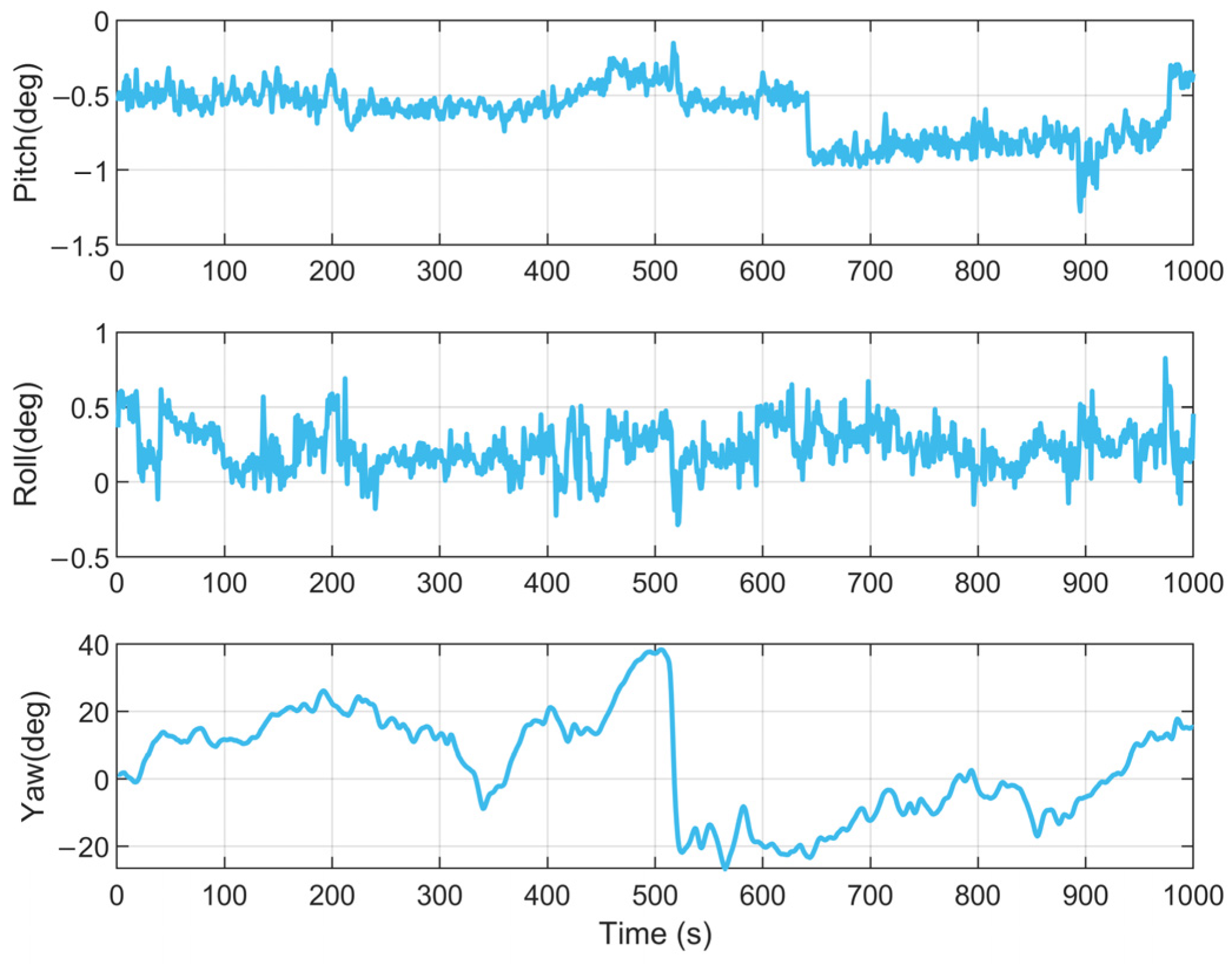
Three 1000 s test segments with different motion characteristics were selected to comprehensively assess the aforementioned initial alignment methods. The first segment (3500–4500 s) featured constant-velocity motion, the second segment (5000–6000 s) involved low-maneuver conditions, and the third segment (8000–9000 s) consisted of high-speed maneuvers. The corresponding trajectory segments are overlapped in Figure 1 for visual reference.

For these three test scenarios, the initial errors for pitch, roll, and yaw angles were set to 30°, 30°, and 80°, respectively. Initial velocity and position errors were both set to zero. The gyroscope bias was configured at 0.02°/h with measurement noise of 0.005°/h, while the accelerometer bias was set to 0.1 mg with measurement noise of 0.1 mg. Consequently, the state noise covariance was established accordingly by Equation (43).

$$\mathbf{Q}=diag{\left[{0.005}^{\circ }/h{\mathbf{I}}_{3\times 1};0.1mg{\mathbf{I}}_{3\times 1}\right]}^2,$$

(43)

Regarding the state-space model, initial attitude covariances were assigned as 10°, 10°, and 27°, with initial velocity covariance at 1 m/s and initial position covariance at 10 m. The time step is specified as 0.005 for all simulations. The state vector in this work is defined with a dimension of 15. The linear filter’s initial state estimation was configured with $\mathsf{\delta }{\widehat{\mathbf{x}}}_0=0_{15\times 1}$. To facilitate computational efficiency comparison, the hardware specifications are explicitly stated: the experiments were conducted on a Lenovo Xiaoxin Air 14 ARE 2020 laptop (Beijing, China) equipped with an AMD Ryzen 5 4600U processor featuring 6 cores, 12 logical processors, and a base clock frequency of 2.10 GHz.

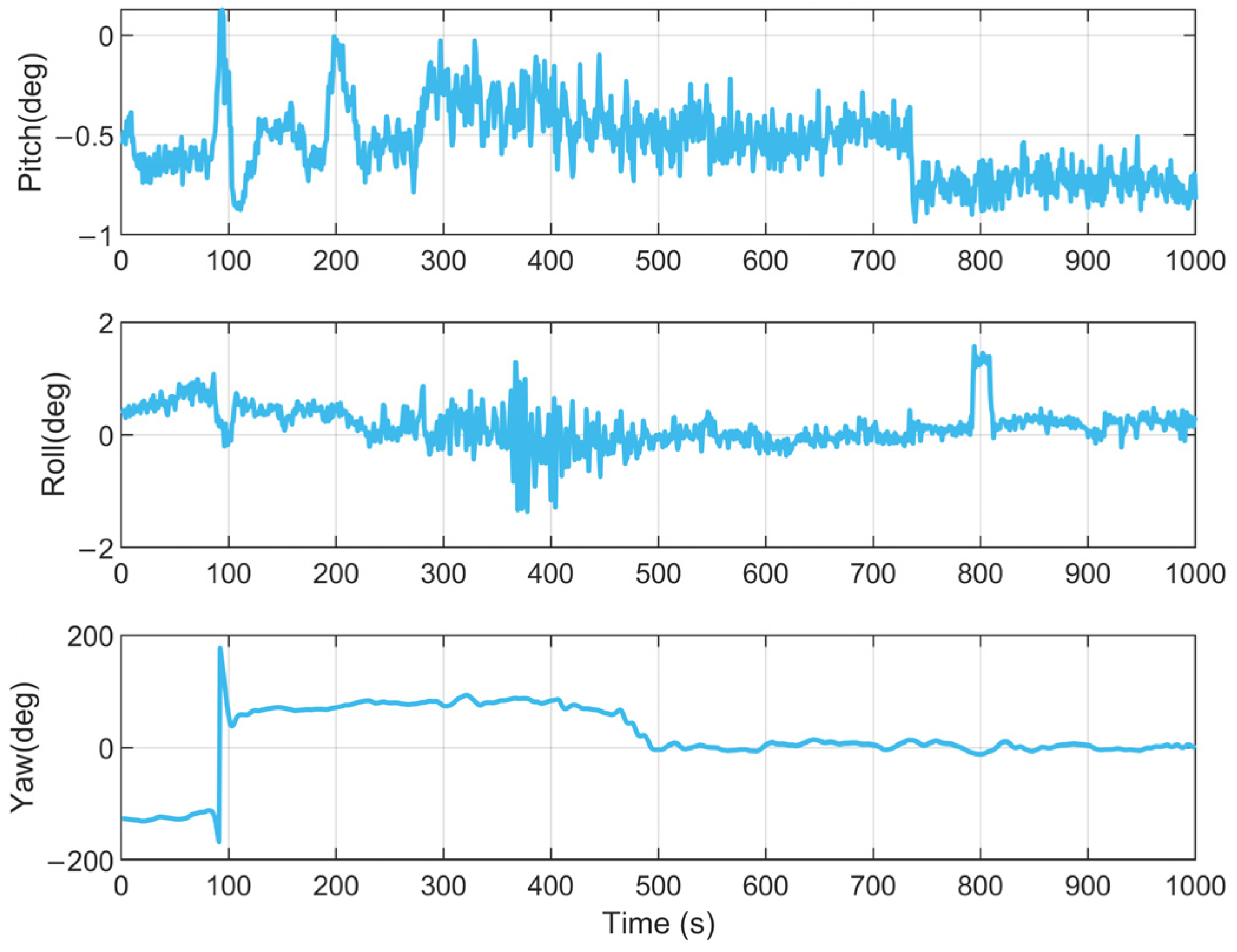
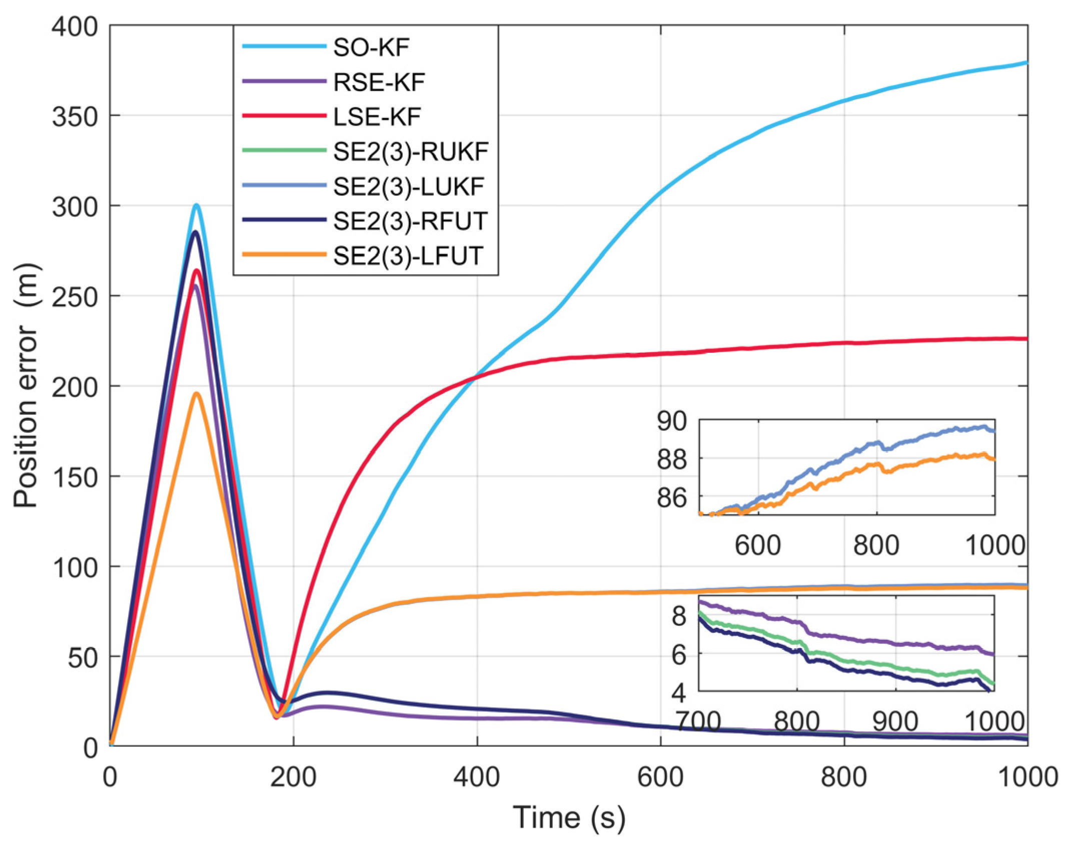
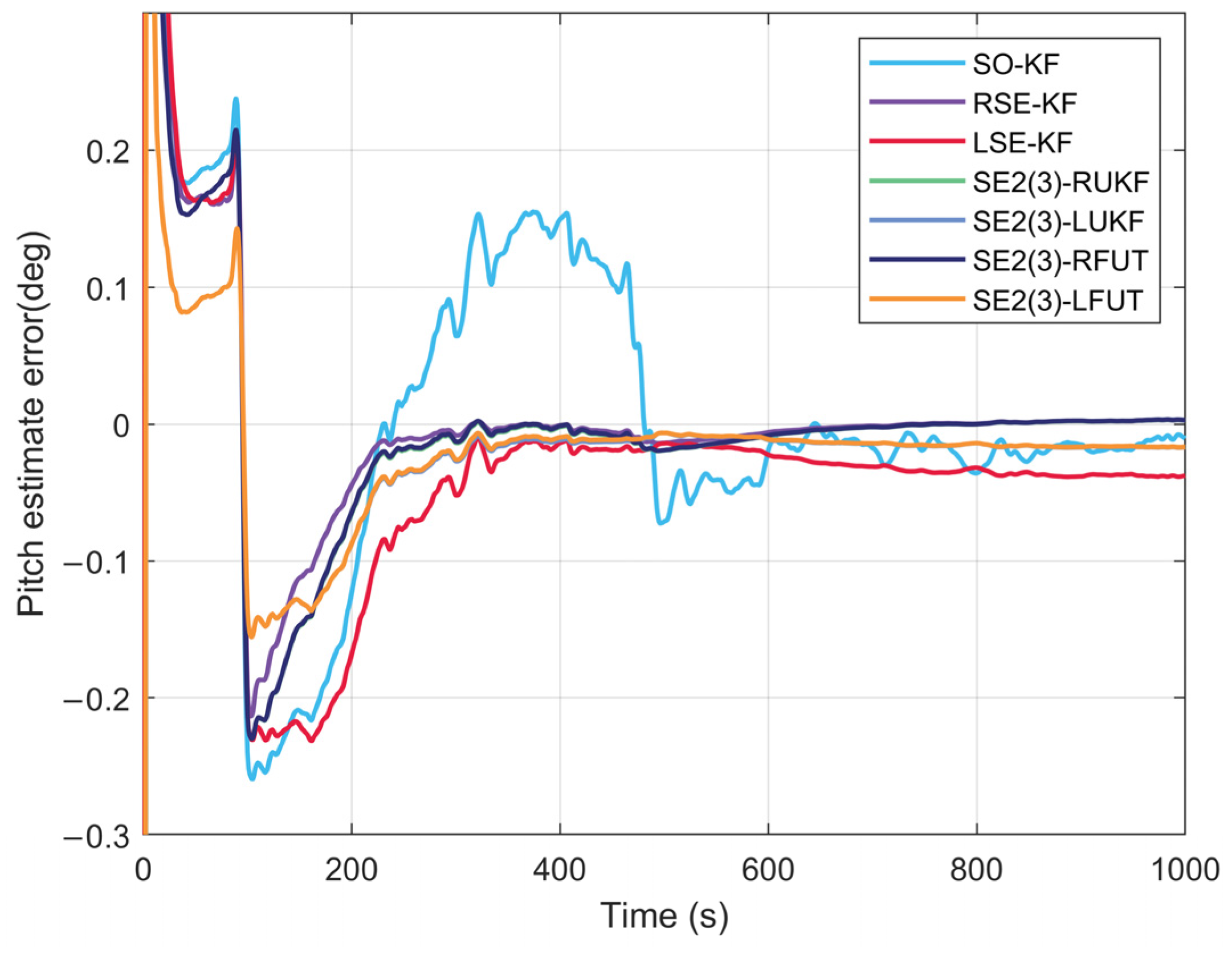
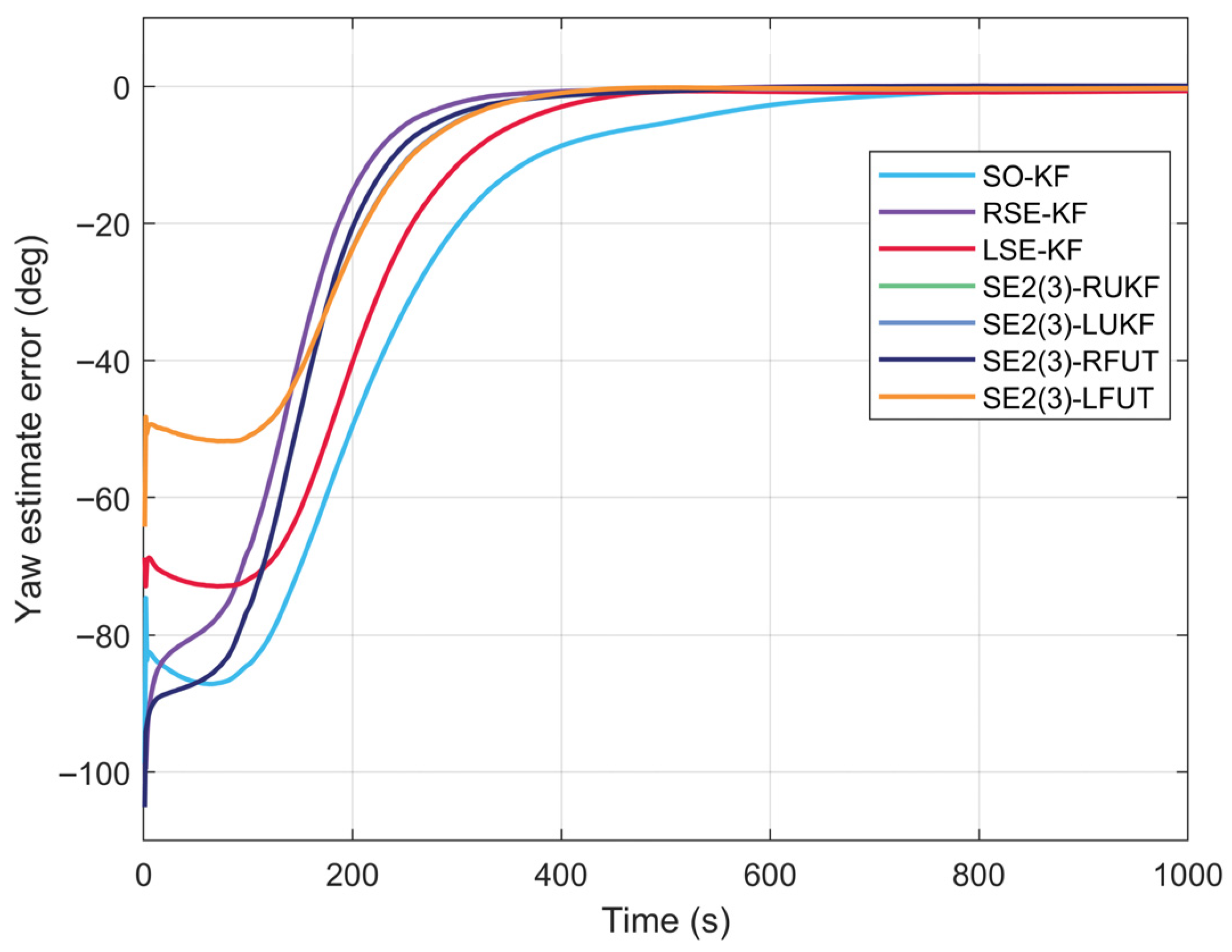
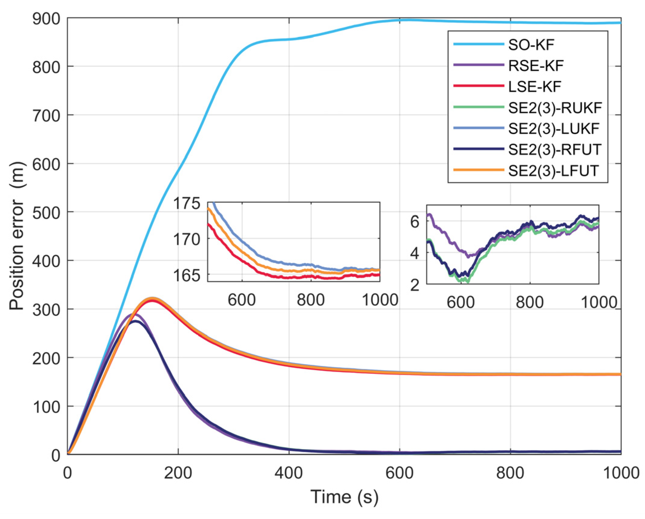
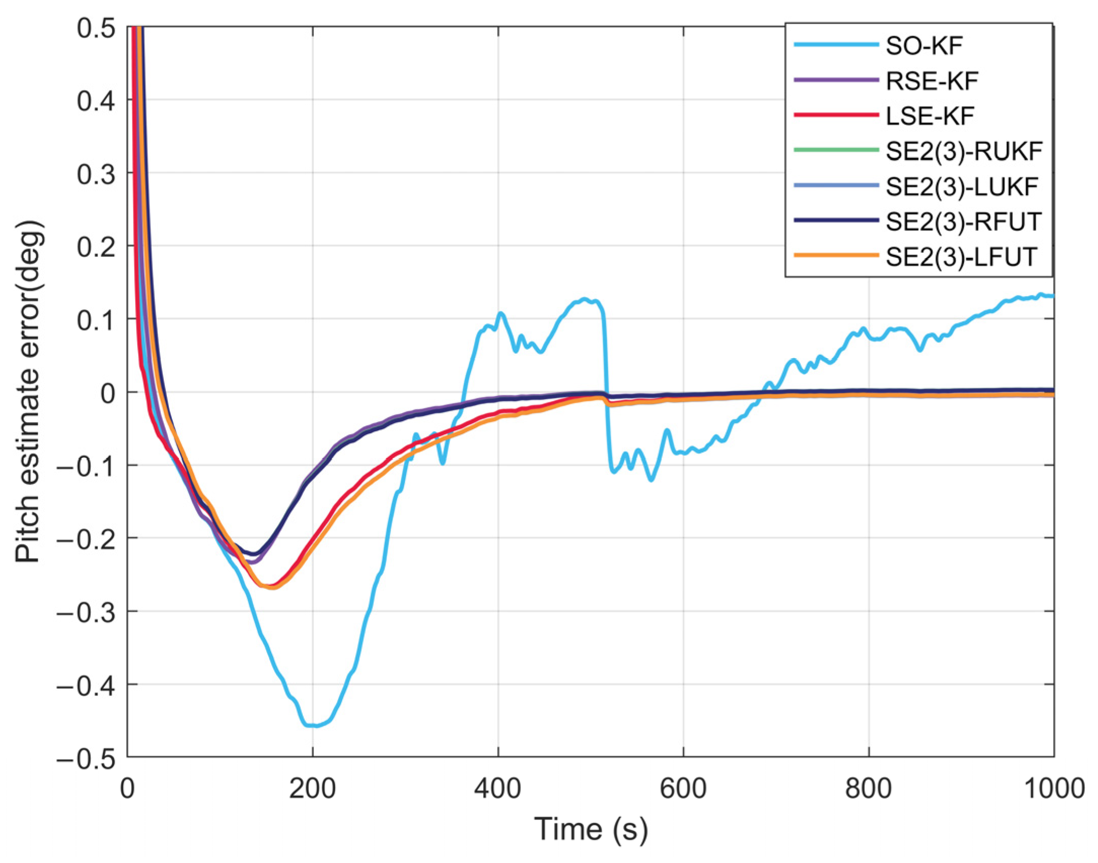
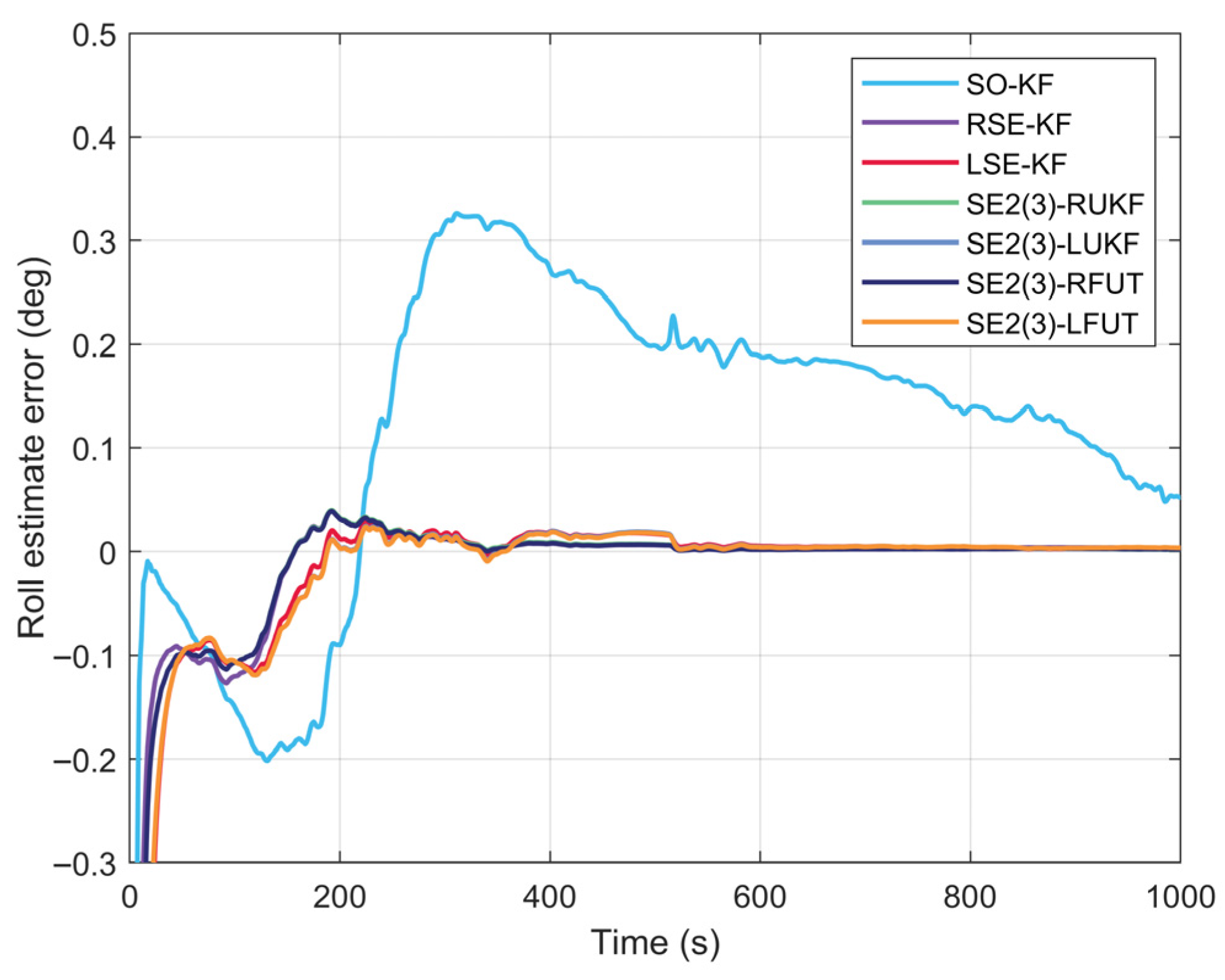
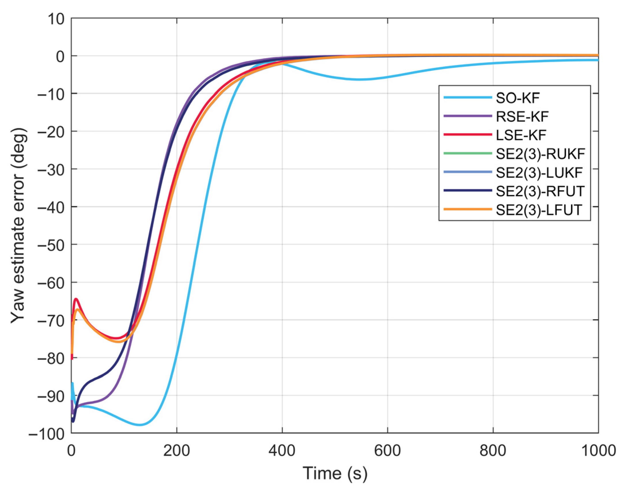
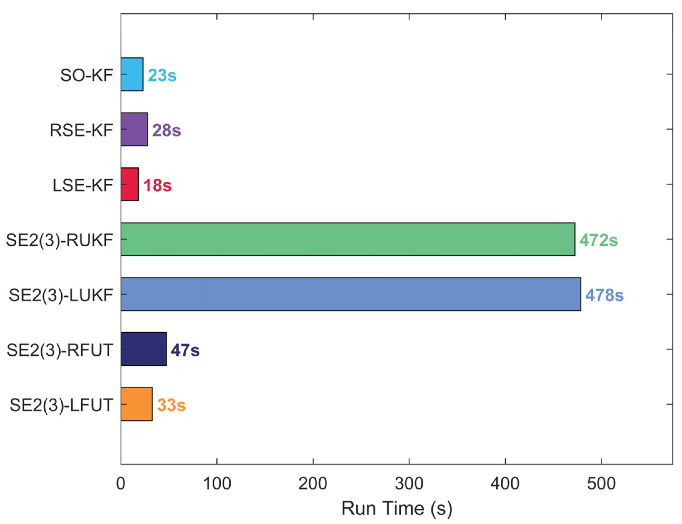
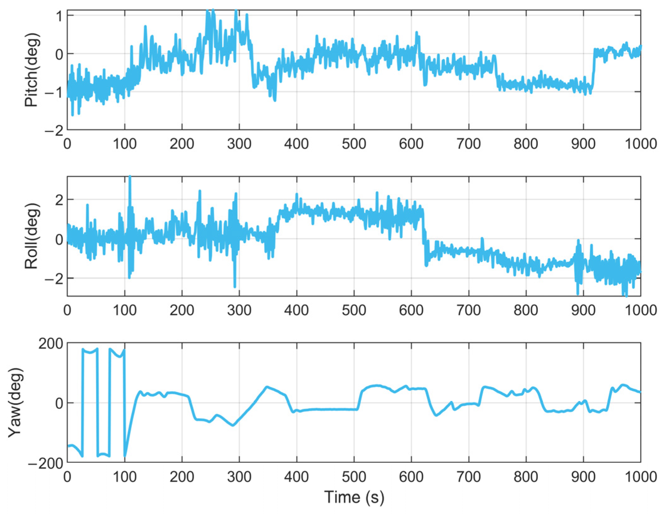
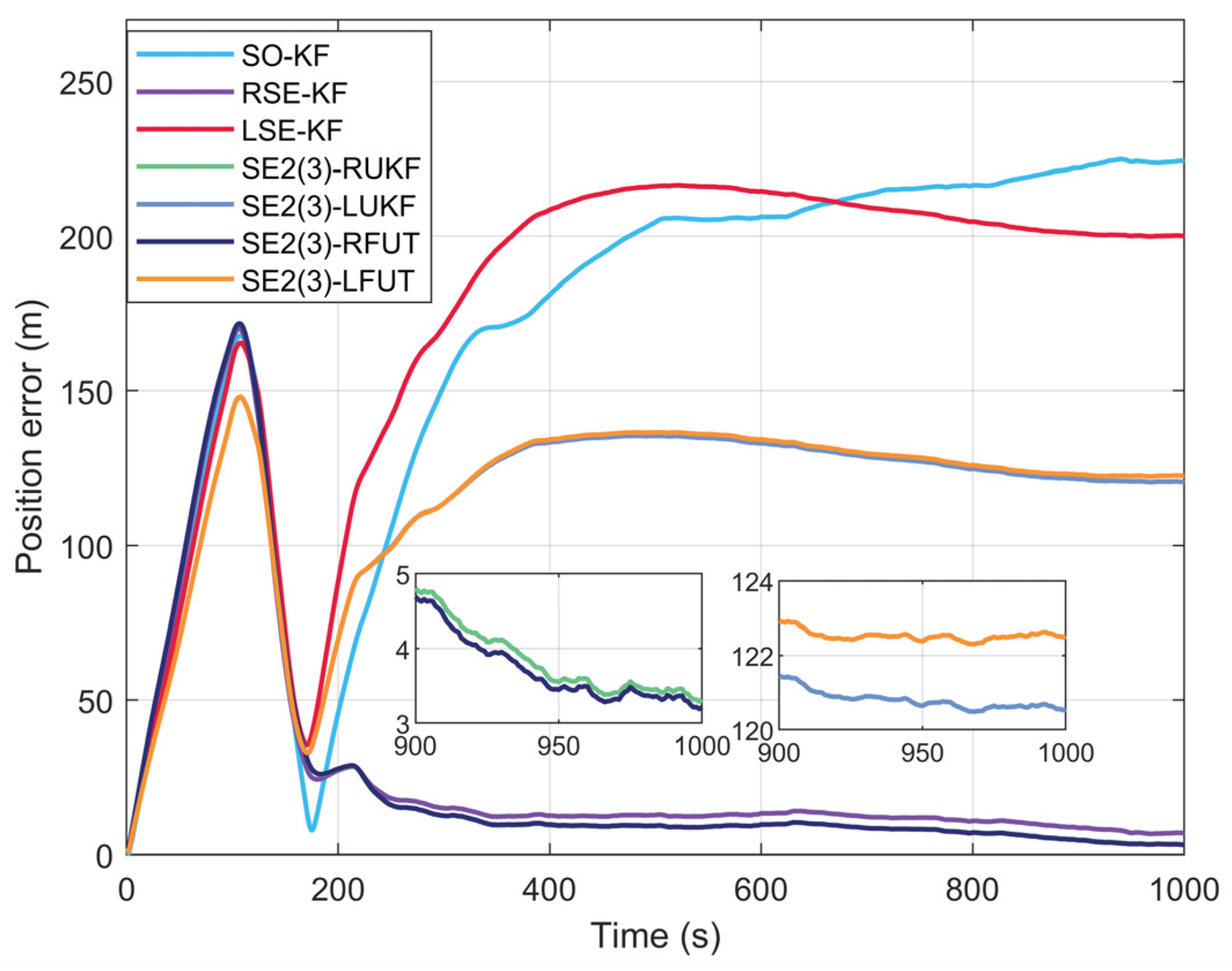
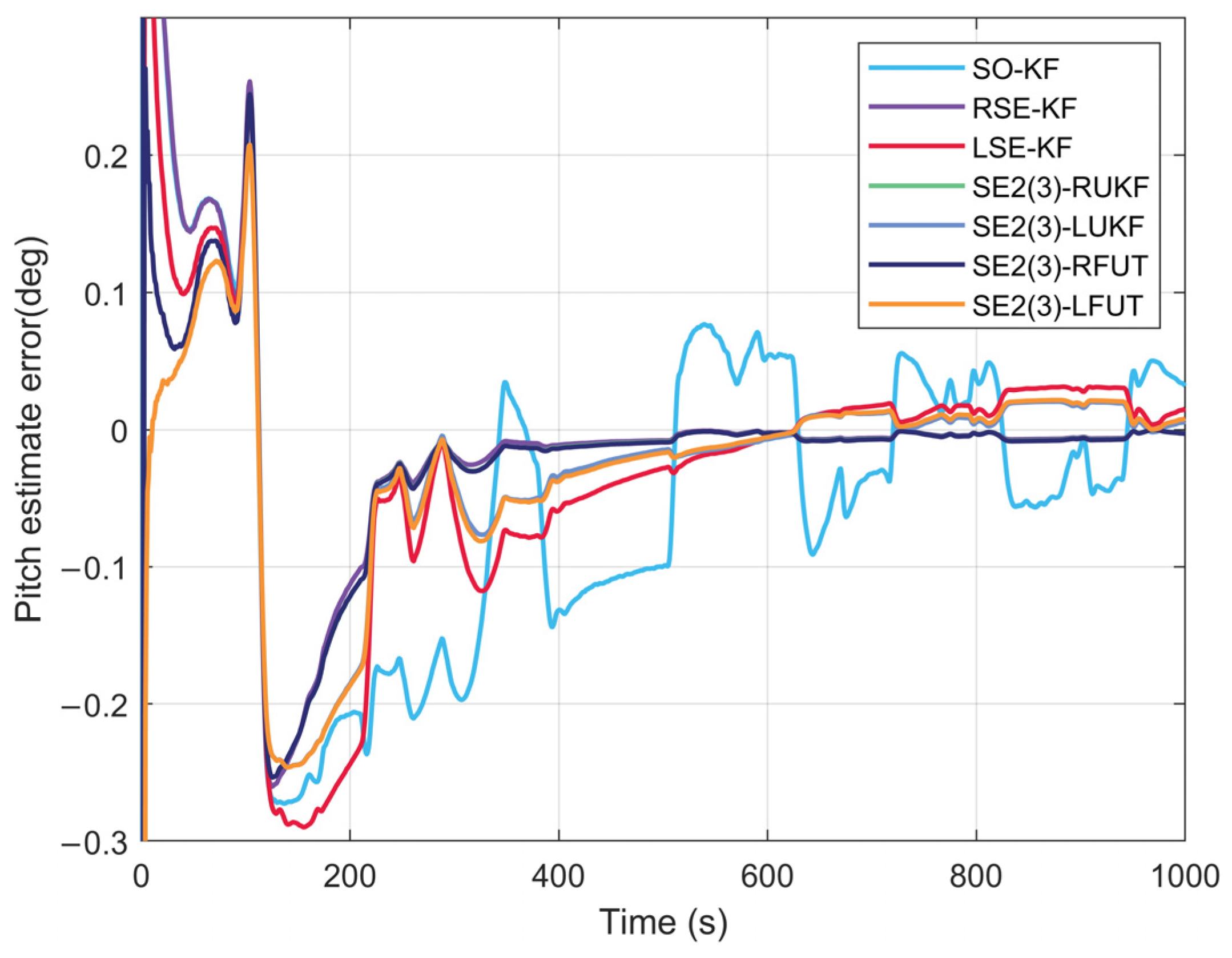
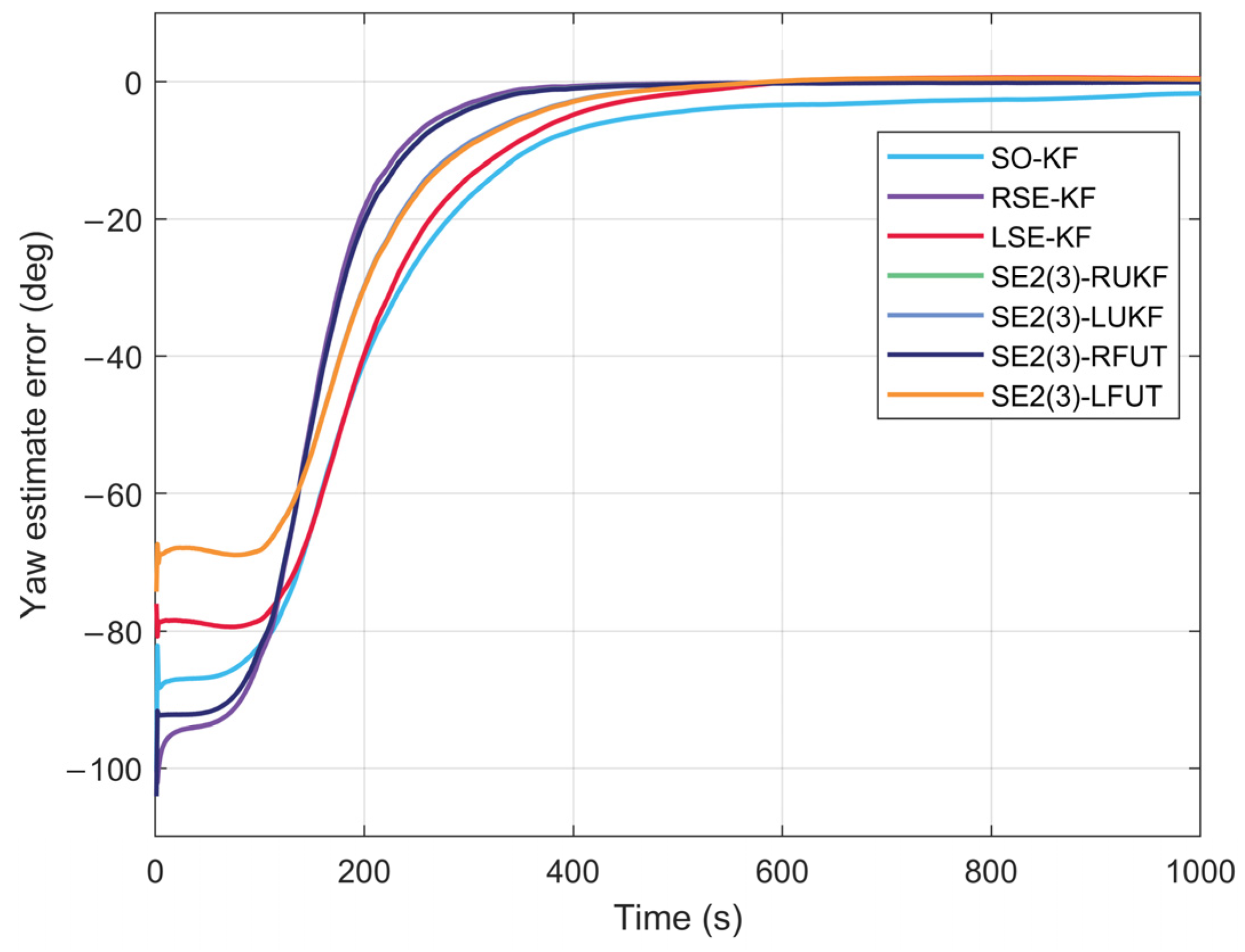
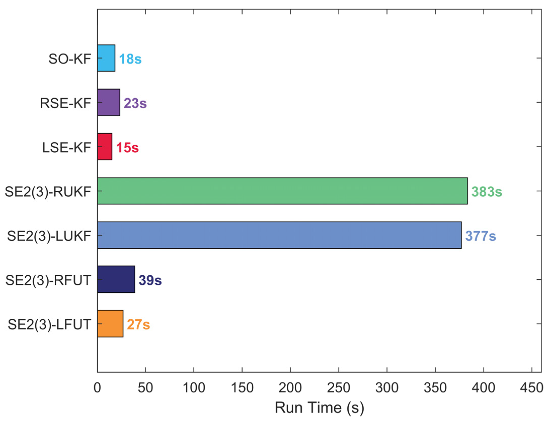
The reference attitude corresponding to the first data segment is presented in Figure 2, while error results are illustrated in Figure 3, Figure 4, Figure 5 and Figure 6. Figure 3 displays the integrated position error during initial alignment of the SINS/DVL system for the first data segment. Figure 4, Figure 5 and Figure 6 demonstrate the attitude estimation errors obtained by different initial alignment methods, respectively. Figure 7 compares the computational time of various initial alignment approaches.

Experimental results demonstrate significant performance differences among filtering methods regarding position error estimation during SINS/DVL initial alignment under constant-velocity conditions. The RSE-KF algorithm demonstrates optimal performance, while the conventional SO-KF exhibits relatively inferior estimation accuracy. This phenomenon aligns with the preceding Lie group theoretical explanation. In DVL-aided measurement scenarios, the measurement model intrinsically corresponds to a right-invariant formulation. When using left-invariant error representation, the linearization of measurement equations unavoidably introduces coupling effects among attitude, velocity, and position estimation errors, ultimately degrading estimation accuracy. In contrast, while the right-invariant error representation still exhibits weak coupling effects among gyro biases, accelerometer biases, and the attitude, velocity, and position states in the state transition matrix, its observation matrix depends solely on global position estimates.

In contrast, the nonlinear filtering methods inherently handle nonlinear equations without linearization-induced approximation errors, theoretically offering superior estimation performance. Experimental results indicate that the FUKF method maintains comparable accuracy to conventional UKF while achieving nearly an order-of-magnitude improvement in computational efficiency. Specifically, FUT requires only 10% of the computational time of traditional UKF, with an acceptable increase of approximately ten seconds compared to linear methods, accompanied by enhanced position estimation accuracy. Regarding attitude estimation (including pitch, roll, and yaw angles), performance differences between nonlinear and conventional linear methods appear relatively minor, suggesting that nonlinear advantages primarily manifest in velocity and position estimation, particularly under significant dynamic or nonlinear conditions.

Overall, under constant-velocity motion, the FUKF not only preserves the accuracy benefits of nonlinear filtering but also achieves substantial computational efficiency improvements through optimized processing flows, establishing an ideal balance between computational cost and estimation accuracy.

The reference attitude for the second data segment is presented in Figure 8, while the corresponding error results are illustrated in Figure 9, Figure 10, Figure 11 and Figure 12. Figure 9 displays the SINS/DVL integrated position error during initial alignment for the second data segment, and Figure 10, Figure 11 and Figure 12 show the attitude estimation errors from different initial alignment methods. Figure 13 compares the computational time across various initial alignment approaches.

Experimental results demonstrate distinct performance variations among the three traditional linear filtering methods in terms of position error estimation during initial alignment under low-speed maneuvering conditions. The RSE-KF exhibits the best performance, followed by the LSE-KF, while the conventional SO-KF performs relatively worst, which aligns with theoretical expectations. Notably, the LSE-KF slightly outperforms nonlinear filtering methods in position estimation accuracy under low-speed maneuvering conditions. This phenomenon can be attributed to two key factors: while low-speed motions (such as minor accelerations or gradual turns) introduce some system dynamics, the overall movement characteristics remain relatively gentle. Under these conditions, LSE-KF benefits from its conservative noise parameter configuration (e.g., employing larger process noise covariance), which enhances its robustness. Furthermore, the SE2(3)-LFUT method’s sensitivity to weak nonlinearities (like minor acceleration disturbances) in low-speed scenarios may lead to slight discrepancies between theoretical models and actual system behavior, whereas LSE-KF’s simpler linearized model proves more adaptable to such operational conditions. This observation suggests that the conservative noise settings of LSE-KF provide a distinct advantage when handling the weak nonlinearities characteristic of low-speed motion scenarios. In contrast, for the right-invariant error representation, estimation accuracy primarily depends on the coupling relationship among global position estimation, gyro drift, and accelerometer bias. Since these factors present relatively low nonlinearity, the experimental results remain consistent with theoretical predictions: the nonlinear filtering methods SE2(3)-RFUT and SE2(3)-RUKF slightly outperform RSE-KF in position error estimation, while differences in attitude angle estimation among the three methods are negligible.

Overall, under low-speed maneuvering conditions, right-invariant error-based nonlinear filtering demonstrates significant advantages. The FUKF not only preserves the precision of traditional nonlinear filtering but also achieves substantial computational efficiency improvements through optimized processing. This presents an enhanced solution for initial alignment in navigation systems under similar scenarios.

Figure 14 presents the reference attitude during initial alignment for the third data segment, with corresponding error results shown in Figure 15, Figure 16, Figure 17 and Figure 18. Figure 15 illustrates the SINS/DVL integrated position error during initial alignment for the third data segment, while Figure 16, Figure 17 and Figure 18 demonstrate the attitude estimation errors obtained from different initial alignment methods. Figure 19 compares the computational time among various initial alignment approaches.

Experimental results demonstrate that nonlinear methods exhibit superior performance compared to linear approaches when using left-invariant error representation. This phenomenon stems from the strongly nonlinear dynamic characteristics under high-speed maneuvering conditions, where the linear approximation in LSE-KF fails to accurately capture the complex system dynamics. In contrast, nonlinear methods effectively preserve the geometric constraints in state space by maintaining complete Lie group structural relationships, thereby achieving better estimation accuracy. The right-invariant error framework further validates the theoretical analysis. For position errors, the SE2(3)-RFUT method yields optimal performance, followed by SE2(3)-RUKF, with both surpassing the linear RSE-KF approach. However, the three methods show comparable performance in attitude angle estimation accuracy. These findings confirm the practical advantages of right-invariant representation in high-speed maneuvering scenarios.

Theoretical and experimental investigations collectively lead to important conclusions: the FUKF algorithm maintains outstanding comprehensive performance throughout initial alignment for all three characteristic motion scenarios, including constant velocity conditions, low-speed maneuvering operations, and high-speed maneuvering situations. By innovatively optimizing state propagation through group-affine properties, the algorithm maintains the accuracy advantages of traditional nonlinear filtering while achieving significant computational complexity reduction. Specifically, this technical solution employs carefully designed numerical computation methods to effectively reduce computational load without compromising estimation accuracy, providing a practical approach for inertial navigation systems with stringent real-time requirements.

4.2. Long-Duration Navigation Performance Evaluation

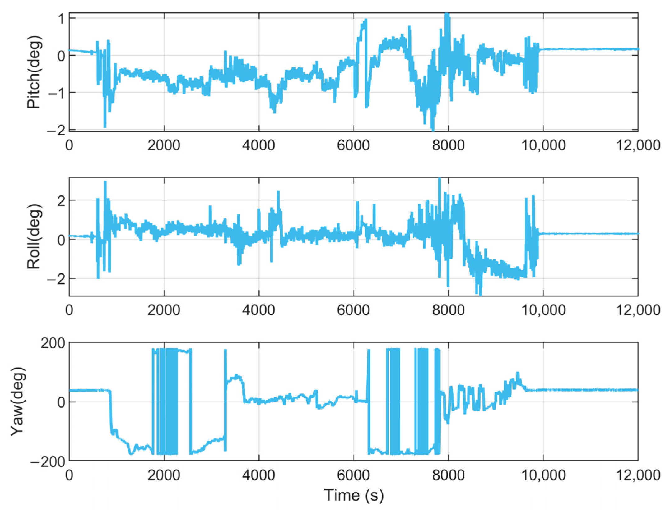
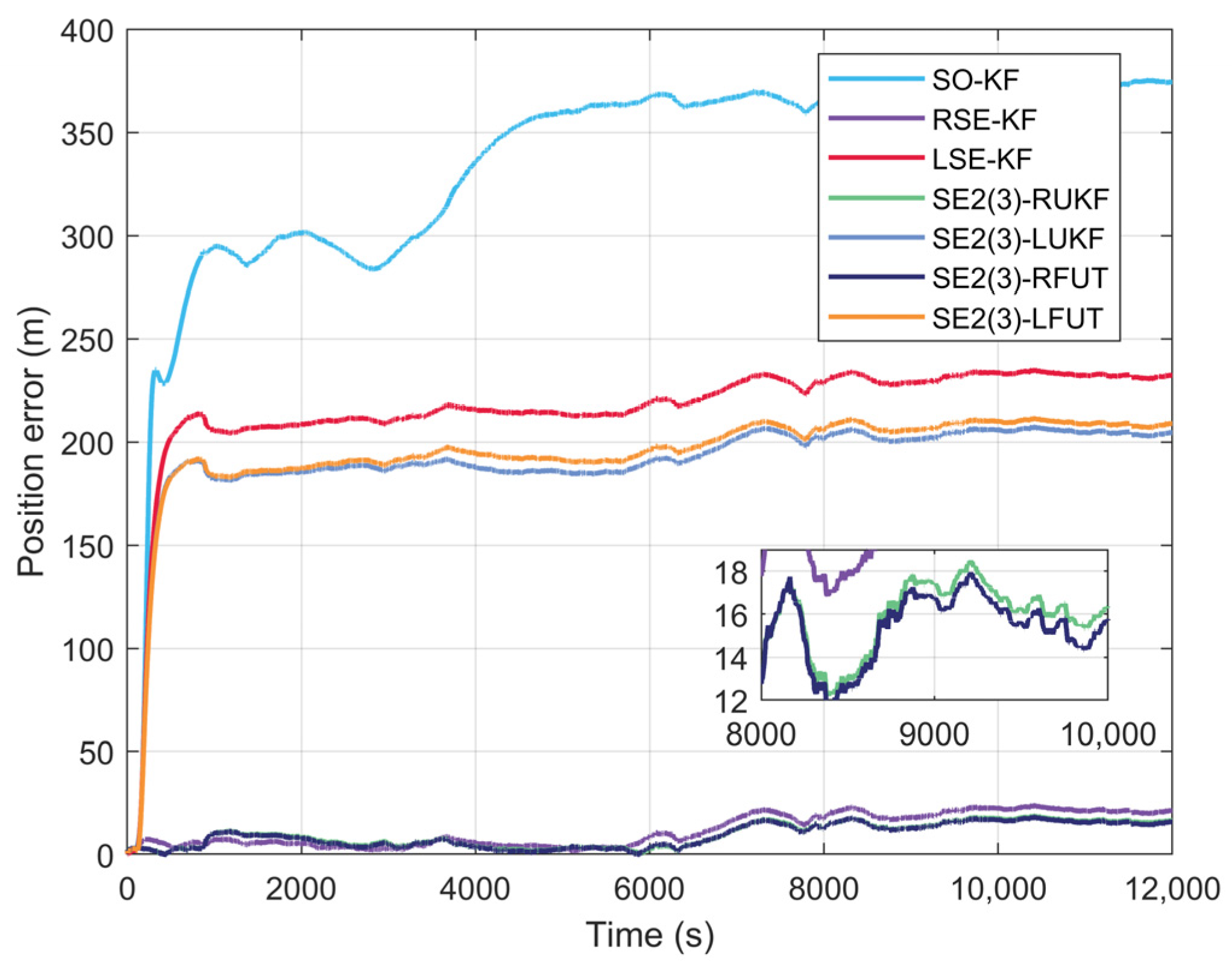
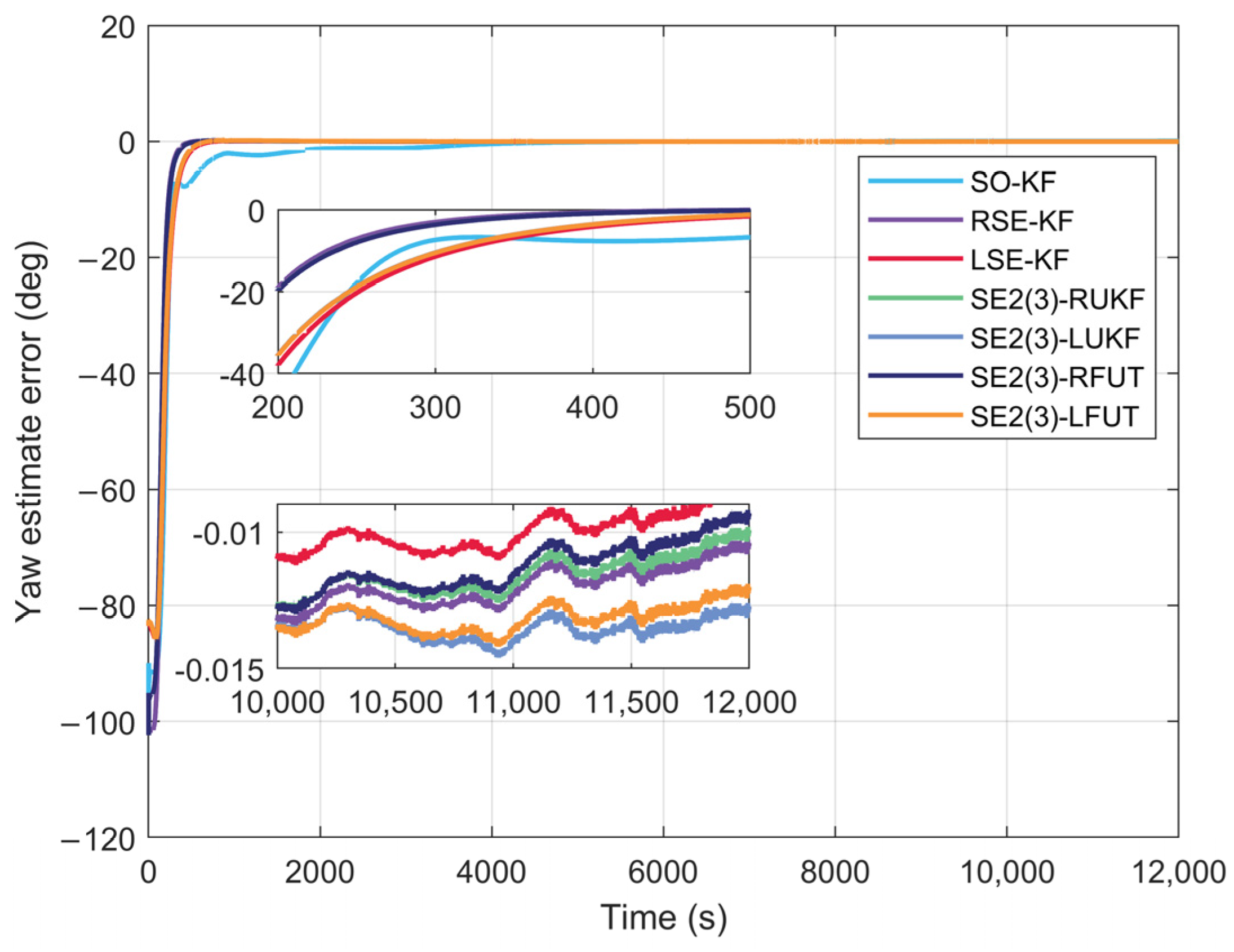
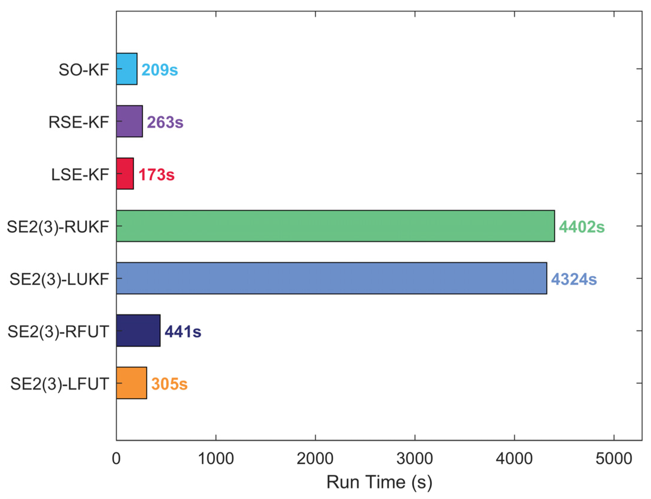
To validate the robustness of the proposed method in extended navigation scenarios, a prolonged 12,000 s navigation test was conducted under consistent parameter configurations. The reference attitude is presented in Figure 20, with corresponding error results illustrated in Figure 21, Figure 22, Figure 23 and Figure 24. Figure 21 displays the SINS/DVL position error, while Figure 22, Figure 23 and Figure 24 present the attitude estimation errors achieved by different initial alignment methods. Figure 25 compares the computational time across various initial alignment approaches.

Experimental results under extended navigation conditions demonstrate consistent algorithm performance characteristics with previous analyses. Regarding position error estimation, the RSE-KF representation demonstrates significant superiority over the LSE-KF, with the conventional SO-KF method exhibiting the poorest performance. For the right-invariant system, all three methods achieve comparable attitude angle estimation accuracy, while SE2(3)-RFUT shows optimal position error performance, followed by SE2(3)-RUKF, both outperforming the linear RSE-KF method—findings that fully align with theoretical predictions. In the left-invariant system, SE2(3)-LFUT and SE2(3)-LUKF demonstrate similar performance, yet both markedly surpass the linear LSE-KF approach. From a computational efficiency perspective, FUT-based methods require substantially less computation time than conventional UKF approaches, maintaining only marginally higher costs than linear methods while significantly improving real-time capabilities.

The proposed navigation system integrates transformed e-frame transformation and group representation with FUKF algorithms. Experimental and theoretical results demonstrate its superior performance. The system achieves excellent accuracy in large-misalignment initial alignment. It also maintains robust performance during long-duration navigation. The proposed approach not only enhances computational efficiency through optimized numerical procedures but also preserves the accuracy advantages of nonlinear filtering. Furthermore, this methodology provides a practical solution for high-precision navigation systems in complex environments, contributing valuable theoretical insights and practical references for advancing inertial navigation technology.

5. Conclusions

The Lie group modeling approach for state errors demonstrates distinct advantages in handling large initial misalignment angles. While traditional linear filtering methods can accomplish alignment tasks, they exhibit inherent theoretical limitations: the state equation based on left-invariant errors fully captures independence with respect to estimated states, yet its corresponding measurement equation retains nonlinear characteristics; the right-invariant error formulation accounts for coupling relationships between gyro drifts, accelerometer biases, and navigation states, but its overall modeling precision remains constrained by linearization assumptions. Nonlinear filtering techniques, particularly the unscented Kalman filter, offer notable benefits by avoiding linearization approximations, though their practical engineering application is hindered by substantial computational burdens.

To address this challenge, this study proposes an improved filtering scheme by the existing FUKF algorithm [29] and integrating a navigation model architecture that satisfies group-affine requirements. The method optimizes sigma-point sampling, performing nonlinear propagation solely on dominant sampling points while employing simplified computations for the remaining points, thereby maintaining estimation accuracy while significantly improving computational efficiency. Systematic validation demonstrates the method’s superior performance across multiple applications, including large misalignment initial alignment and SINS/DVL integrated navigation, particularly excelling in computational efficiency. The proposed approach reduces computation time by 90%. It should be noted that this work primarily entails the innovative application of the existing FUT algorithm within a specific navigation system modeling framework rather than the original development of the algorithm itself. The proposed framework demonstrates compatibility with such error compensation through state vector augmentation (e.g., incorporating lever-arm parameters in $S{E}_2(3)$), which may constitute a promising direction for future research. Meanwhile, future research could explore integrating probabilistic risk assessment methods (e.g., ANP and fuzzy evaluation models [31]) to enhance fault tolerance in SINS/DVL fusion under uncertain environmental conditions.

References

1. Paull, L.; Saeedi, S.; Seto, M.; Li, H. AUV Navigation and Localization: A Review. IEEE J. Ocean. Eng. 2014, 39, 131–149. [Google Scholar] [CrossRef]
2. Chen, K.-Y.; Huang, N.-Y.; Su, W.; Cheng, E. An Underwater Concealed Navigation and Positioning Method Based on SINS and LBL. J. Unmanned Undersea Syst. 2022, 30, 37–43. [Google Scholar]
3. Liu, K.-R. Research on Deep-Sea Ultra-Short Baseline Positioning Algorithm Based on Underwater Acoustic Ultra-Wideband Signal. Ph.D. Thesis, Hainan University, Haikou, China, 2020. [Google Scholar]
4. Li, W.-J.; Wang, Z.-J.; Sun, Z.; Zhang, S.-M. Sound Velocity Correction Method for Ultra-Short Baseline Based on Depth Constraint. J. Navig. Position. 2022, 10, 40–45. [Google Scholar]
5. Wang, B.; Liu, J.-Y.; Liu, P.-J. Overview of SINS/DVL Integrated Navigation Technology. J. Navig. Position. 2020, 8, 1–6+22. [Google Scholar] [CrossRef]
6. Zhao, J.-B.; Ge, X.-Y.; Feng, X.-L.; Zhou, H.-K. Survey of Underwater SINS/DVL Integrated Navigation Technology. J. Unmanned Undersea Syst. 2018, 26, 2–9. [Google Scholar]
7. Zhu, Z. Research on Underwater SINS/DVL Integrated Navigation Technology. Master’s Thesis, China Three Gorges University, Yichang, China, 2024. [Google Scholar] [CrossRef]
8. Lu, D.-H.; Song, S.-L.; Wang, J.; Cai, Y.-X.; Shen, H.-H. Development Review of Underwater SINS/DVL Integrated Navigation Technology. Control Theory Appl. 2022, 39, 1159–1170. [Google Scholar]
9. Barrau, A.; Bonnabel, S. Intrinsic Filtering on SO(3) with Discrete-Time Observations. In Proceedings of the 52nd IEEE Conference on Decision and Control, Florence, Italy, 10–13 December 2013; pp. 3255–3260. [Google Scholar] [CrossRef]
10. Bonnabel, S.; Martin, P.; Salaün, E. Invariant Extended Kalman Filter: Theory and Application to a Velocity-Aided Attitude Estimation Problem. In Proceedings of the 48h IEEE Conference on Decision and Control, Shanghai, China, 15–18 December 2009; pp. 1297–1304. [Google Scholar] [CrossRef]
11. Barrau, A.; Bonnabel, S. Invariant Filtering for Pose EKF-SLAM Aided by an IMU. In Proceedings of the 2015 54th IEEE Conference on Decision and Control, Osaka, Japan, 15–18 December 2015; pp. 2133–2138. [Google Scholar] [CrossRef]
12. Barrau, A.; Bonnabel, S. An EKF-SLAM Algorithm with Consistency Properties. arXiv 2015, arXiv:1510.06263. [Google Scholar] [CrossRef]
13. Barrau, A.; Bonnabel, S. Alignment Method for an Inertial Unit. U.S. Patent 15/037,653, 6 October 2016. [Google Scholar]
14. Barrau, A.; Bonnabel, S. The Invariant Extended Kalman Filter as a Stable Observer. IEEE Trans. Autom. Control 2017, 62, 1797–1812. [Google Scholar] [CrossRef]
15. Brossard, M.; Bonnabel, S.; Barrau, A. Invariant Kalman Filtering for Visual Inertial SLAM. In Proceedings of the 2018 21st International Conference on Information Fusion, Cambridge, UK, 10–13 July 2018; pp. 2021–2028. [Google Scholar] [CrossRef]
16. Barrau, A.; Bonnabel, S. A Mathematical Framework for IMU Error Propagation with Applications to Pre-integration. In Proceedings of the 2020 IEEE International Conference on Robotics and Automation, Paris, France, 31 May–31 August 2020; pp. 5732–5738. [Google Scholar] [CrossRef]
17. Barrau, A. Non-linear State Error Based Extended Kalman Filters with Applications to Navigation. Ph.D. Thesis, Department of Automatic, Mines ParisTech, Paris, France, 2015. [Google Scholar]
18. Chang, L.; Di, J.; Qin, F. Inertial-based Integration with Transformed INS Mechanization in Earth Frame. IEEE/ASME Trans. Mechatron. 2022, 27, 1738–1749. [Google Scholar] [CrossRef]
19. Chang, L.; Bian, Q.; Zuo, Y.; Zhou, Q. SINS/GNSS-integrated Navigation Based on Group Affine SINS Mechanization in Local-level Frame. IEEE/ASME Trans. Mechatron. 2023, 28, 2471–2482. [Google Scholar] [CrossRef]
20. Chang, L.; Tang, H.; Hu, G.; Xu, J. SINS/DVL Linear Initial Alignment Based on Lie Group SE3(3). IEEE Trans. Aerosp. Electron. Syst. 2023, 59, 7203–7217. [Google Scholar] [CrossRef]
21. Chang, L.; Luo, Y. Log-linear Error State Model Derivation Without Approximation for INS. IEEE Trans. Aerosp. Electron. Syst. 2023, 59, 2029–2035. [Google Scholar] [CrossRef]
22. Du, S.; Huang, Y.; Lin, B.; Qian, J.; Zhang, Y. A Lie Group Manifold-Based Nonlinear Estimation Algorithm and Its Application to Low-Accuracy SINS/GNSS Integrated Navigation. IEEE Trans. Instrum. Meas. 2022, 71, 1002927. [Google Scholar] [CrossRef]
23. Chirikjian, G.S. Stochastic Models, Information Theory, and Lie Groups: Analytic Methods and Modern Applications; Springer: Berlin/Heidelberg, Germany, 2011; Volume 2. [Google Scholar]
24. Barfoot, T.D. State Estimation for Robotics; Cambridge University Press: Cambridge, UK, 2017. [Google Scholar]
25. Solà, J.; Deray, J.; Atchuthan, D. A Micro Lie Theory for State Estimation in Robotics. arXiv 2018, arXiv:1812.01537. [Google Scholar]
26. Hartley, R.; Ghaffari, M.; Eustice, R.M.; Grizzle, J.W. Contact Aided Invariant Extended Kalman Filtering for Robot State Estimation. Int. J. Robot. Res. 2020, 39, 402–430. [Google Scholar] [CrossRef]
27. Mao, J.; Lian, J.; Hu, X. Strapdown Inertial Navigation Algorithms Based on Lie Group. J. Navigat. 2017, 70, 165–183. [Google Scholar] [CrossRef]
28. Tang, H.; Xu, J.; Chang, L.; Shi, W.; He, H. Invariant Error-based Integrated Solution for SINS/DVL in Earth Frame: Extension and Comparison. IEEE Trans. Instrum. Meas. 2023, 72, 9500617. [Google Scholar] [CrossRef]
29. Jin, Y.; Zhang, W.-A.; Tang, J.; Sun, H.; Shi, L. A Nonlinear Filter for Pose Estimation Based on Fast Unscented Transform on Lie Groups. IEEE Robot. Autom. Lett. 2024, 9, 10431–10438. [Google Scholar] [CrossRef]
30. Luo, Y.; Guo, C.; You, S.; Hu, J.; Liu, J. SE2(3) Based Extended Kalman Filtering and Smoothing Framework for Inertial-integrated Navigation. arXiv 2021, arXiv:2102.12897. [Google Scholar]
31. Chen, X.; Liu, S.; Liu, R.W.; Wu, H.; Han, B.; Zhao, J. Quantifying Arctic Oil Spilling Event Risk by Integrating an Analytic Network Process and Fuzzy Comprehensive Evaluation Model. Ocean Coast. Manag. 2022, 228, 106326. [Google Scholar] [CrossRef]
Figure 1. Mulan Lake Test Trajectory.
Jmse 13 01682 g001
Figure 2. Reference attitude during initial alignment for the first data segment.
Jmse 13 01682 g002
Figure 3. Position error during initial alignment for the first data segment.
Jmse 13 01682 g003
Figure 4. Pitch angle during initial alignment for the first data segment.
Jmse 13 01682 g004
Figure 5. Roll angle during initial alignment for the first data segment.
Jmse 13 01682 g005
Figure 6. Yaw angle during initial alignment for the first data segment.
Jmse 13 01682 g006
Figure 7. Computational time comparison for the first data segment.
Jmse 13 01682 g007
Figure 8. Reference attitude during initial alignment for the second data segment.
Jmse 13 01682 g008
Figure 9. Position error during initial alignment for the second data segment.
Jmse 13 01682 g009
Figure 10. Pitch angle during initial alignment for the second data segment.
Jmse 13 01682 g010
Figure 11. Roll angle during initial alignment for the second data segment.
Jmse 13 01682 g011
Figure 12. Yaw angle during initial alignment for the second data segment.
Jmse 13 01682 g012
Figure 13. Computational time comparison for the second data segment.
Jmse 13 01682 g013
Figure 14. Reference attitude during initial alignment for the third data segment.
Jmse 13 01682 g014
Figure 15. Position error during initial alignment for the third data segment.
Jmse 13 01682 g015
Figure 16. Pitch angle during initial alignment for the third data segment.
Jmse 13 01682 g016
Figure 17. Roll angle during initial alignment for the third data segment.
Jmse 13 01682 g017
Figure 18. Yaw angle during initial alignment for the third data segment.
Jmse 13 01682 g018
Figure 19. Computational time comparison for the third data segment.
Jmse 13 01682 g019
Figure 20. Reference attitude during long-duration navigation.
Jmse 13 01682 g020
Figure 21. Position error during long-duration navigation.
Jmse 13 01682 g021
Figure 22. Pitch angle during long-duration navigation.
Jmse 13 01682 g022
Figure 23. Roll angle during long-duration navigation.
Jmse 13 01682 g023
Figure 24. Yaw angle during long-duration navigation.
Jmse 13 01682 g024
Figure 25. Computational time comparison for long-duration navigation.
Jmse 13 01682 g025