Abstract
Accurate wave forecasting under typhoon conditions is essential for coastal safety in the Pearl River Estuary. This study explores the use of Random Forest (RF) and Long Short-Term Memory (LSTM) models to predict significant wave heights, using SWAN-simulated data from 87 historical typhoon events. Ten representative typhoons were reserved for independent testing. Results show that the LSTM model outperforms RF in 3 h forecasts, achieving a lower mean RMSE and higher R2, particularly in capturing wave peaks under highly dynamic conditions. For 6 h forecasts, both models exhibit decreased accuracy, with RF performing slightly better in stable scenarios, while LSTM remains more responsive in complex wave evolution. Generalization tests at three nearby stations demonstrate that both models, especially LSTM, retain strong predictive skill beyond the training location. These findings highlight the potential of combining numerical wave models with machine learning for short-term, data-driven wave forecasting in typhoon-prone and observation-sparse regions. The study also points to future improvements through integration of wind field predictors, model updating strategies, and ensemble meteorological data.
1. Introduction
Short-term wave forecasting is essential for ensuring the safety and efficiency of ship navigation, coastal engineering operations, and disaster mitigation efforts, especially under extreme weather conditions [1,2]. Accurate forecasts can substantially reduce the risks posed by rapidly evolving sea states, particularly during tropical cyclones, which often generate extreme wave conditions and threaten coastal infrastructure and maritime activities [3].
Numerical models are widely used in studying and forecasting the significant wave height (Hs) [4]. Well-established models such as the Simulating Waves Nearshore (SWAN) model [5], MIKE 21 [6], and Delft-3D [7] have been extensively applied in predicting Hs in coastal and nearshore regions, and have demonstrated good performance under typhoon-induced extreme wave conditions [8,9,10]. In operational practice, however, these models are more often applied in hindcast mode to reconstruct past wave conditions, as their real-time use is limited by high computational cost, the need for extensive input data, and the time required for setup and calibration [11]. This limitation creates a clear need for alternative approaches capable of producing rapid forecasts. Machine learning (ML) models, once trained, can generate predictions almost instantaneously, making them a promising complement to numerical models for short-term wave forecasting.
In recent years, ML techniques have shown great promise in coastal and ocean engineering applications [12,13,14,15], especially for forecasting wave conditions [16,17,18]. A variety of models, such as support vector machines (SVMs), random forest (RF), artificial neural network (ANN), and recurrent architectures like long short-term memory (LSTM) networks, have been successfully employed to capture the dynamic behavior of ocean waves [19,20,21,22,23,24]. For example, ANN has been applied to estimate wave breaking height using environmental parameters [25]. RF, ANN, and SVMs have been compared for swell occurrence prediction, with RF achieving the highest accuracy [26]. Jörges et al. [27] found that incorporating bathymetric features alongside meteorological inputs can significantly enhance the accuracy of LSTM-based wave height forecasting models. Lu et al. [28] proposed a hybrid deep learning framework named Extreme-Enhanced LSTM-NBEATS, which achieved high accuracy in 24 h Hs forecasts, particularly under extreme wave conditions in the Gulf of Mexico. More recently, Tan et al. [29] developed a Swin Transformer-based deep learning model for regional wave height prediction. With a carefully designed architecture, the model accurately reproduces wave heights up to 24 h in advance across the target region. Overall, ML approaches can improve wave height prediction accuracy while reducing computational cost [30,31]. In additions, previous studies have demonstrated the strong performance of RF in short-term environmental forecasting [32] and the ability of LSTM to model dynamic wave processes with high accuracy [27]. Therefore, in this study, RF and LSTM are selected as two representative and widely used ML models to evaluate and compare their predictive capabilities for significant wave height forecasting. These two models represent distinct methodological paradigms (tree-based ensemble learning vs. recurrent neural networks), enabling a meaningful comparative evaluation of their predictive capabilities within the same experimental framework.
Despite recent progress, the effectiveness of data-driven ML models for wave prediction still largely depends on the availability of sufficient observational data for training [28,33,34]. Most existing applications have been conducted in open-ocean or well-instrumented coastal environments where long-term buoy records are available. For example, an innovative deep-learning framework combining Variational Mode Decomposition, LSTM, and Transfer Learning has been successfully applied to Hs forecasting using buoy measurements and ECMWF wind data [35]. Similarly, generalized machine learning approaches such as ANN, SNN, XGBoost, and LightGBM have been trained on large coastal datasets from 47 stations along the North American coast and evaluated on 6 independent stations [36]. To mitigate the limitation of sparse in situ data, especially during extreme weather events, researchers have begun integrating physics-based numerical simulations with ML algorithms to improve prediction skill in data-scarce but high-risk scenarios [11,37,38]. One approach involves using data generated from established wave models, such as SWAN, to train surrogate ML models that can approximate wave conditions with reduced computational demand. For instance, Chen et al. [39] developed a surrogate prediction framework based on the random forest algorithm, trained on spatial wave data derived from SWAN simulations, which enabled efficient wave condition forecasting without running the full numerical model. Expanding on this idea, Chen et al. [40] demonstrated that coupling SWAN with machine learning techniques, including backpropagation neural networks and random forest regression, can significantly improve the prediction of wave heights under typhoon conditions, outperforming the original SWAN model in both accuracy and responsiveness.
In contrast, research in the offshore waters adjacent to the Pearl River Estuary (PRE) in the northern South China Sea (the northern part of the South China Sea) remains relatively limited, particularly under typhoon conditions when reliable Hs measurements are scarce due to safety constraints and instrument failures. This region is one of the most economically developed and densely populated coastal areas in China, with intensive maritime traffic, port operations, and coastal infrastructure. The scarcity of accurate and timely wave forecasts under extreme conditions poses substantial risks to navigation safety, coastal engineering, and disaster preparedness. These limitations posed a significant challenge for developing robust short-term forecasting systems in such high-risk areas.
This study aims to develop a hybrid prediction framework that integrates high-resolution SWAN simulations with RF and LSTM to improve short-term significant wave height forecasting in data-scarce estuarine environments. The framework is trained and validated using SWAN-simulated wave data from multiple historical typhoon events in the PRE, a region in the northern South China Sea where frequent tropical cyclones generate complex and highly variable wave fields. The novelty of this study lies in systematically evaluating both temporal- and spatial-generalization performance under typhoon conditions and revealing the stage-dependent predictive behavior of RF and LSTM across multiple events. This approach provides a transferable methodology for enhancing wave forecasting capability in similar coastal regions worldwide. This paper is organized as follows: Section 2 describes the study area, SWAN model setup, machine learning model architectures, and experimental design. Section 3 presents the results of wave height prediction performance and model generalization across typhoon events. Section 4 discusses the findings, and Section 5 concludes the study with key implications and future perspectives.
2. Materials and Methods
2.1. Study Area, Typhoons and Data
This study focuses on the northern South China Sea, with particular emphasis on the coastal waters surrounding the PRE. This region is frequently influenced by tropical cyclones that traverse or make landfall along the southern coast of China, inducing complex and extreme wave conditions. To ensure accurate wave modeling, especially during typhoon events, the computational domain was designed to extend beyond PRE. Specifically, the model domain ranges from 13° N to 30° N and from 105° E to 125° E, as shown in Figure 1. This domain configuration ensures that tropical cyclones entering the region at least 24 h prior to expected landfall are fully contained within the simulation boundaries. This spatial extension helps avoid artificial edge effects and ensures complete coverage of extreme wave development and propagation.
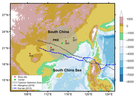
Figure 1.
Study area and observational stations in the northern South China Sea.
The green dot marks the center of the typhoon selection region (QF308), with a 350 km radius used to confirm historical typhoon events. Red dots indicate the locations of four buoys (QF303, QF304, QF306, and QF307). Two typhoons Mangkhut (2018, gray line) and Kai-tak (2012, blue line) are selected for SWAN model validation, with their tracks displayed across the South China Sea.
Wind forcing data were obtained from the ERA5 wind reanalysis dataset provided by the European Centre for Medium-Range Weather Forecasts (ECMWF) [41]. With hourly temporal resolution and 0.25 degree spatial resolution, ERA5 has been widely adopted in wave modeling applications [42]. In this paper, a total of 87 typhoons were selected based on the following criteria: the tropical cyclone must have passed through a circular region with a radius of 350 km centered at 114.797° E, 21.890° N (as marked in Figure 1), and the maximum 10 m wind speed within this region must have exceeded 32.7 m/s, which is the threshold for classification as a typhoon. All thyphoons name and time list in Table A1 of Appendix A. This selection ensures that all included events had a direct in fluence on the Pearl River Estuary and its surrounding waters, and represent a wide range of extreme wave-generating conditions. The corresponding ERA5 wind fields for these typhoon events were used as dynamic forcing inputs to drive the SWAN model and simulate the extreme sea states.
Bathymetric data were constructed by merging the ETOPO1 ocean bathymetry dataset from the National Oceanic and Atmospheric Administration (NOAA) [43] with high-resolution measured depth data, providing detailed underwater topography essential for accurate nearshore wave transformation. Buoy observations used for model validation were obtained from in situ wave buoy datasets provided by the South China Sea Branch of the State Oceanic Administration (SCSB-SOA), China. The data were accessed through the official data portal [44], and include long-term measurements of significant wave height, peak wave period, and wind speed. In this study, four buoy stations identified as QF303, QF304, QF306, and QF307 are involved in the model validation. These buoy sites are positioned in the northern South China Sea and provide high-resolution observational records, which are used to validate the accuracy of the model (Figure 1).
2.2. SWAN Model
2.2.1. Model Description
The SWAN model is the third-generation spectral wave model, which is a spectral wave model that captures the dynamics of such high-frequency waves when they are nearshore. It was employed to simulate the evolution of wave fields under typhoon forcing, in this paper. SWAN solves the wave-action balance equation in the frequency–direction domain, accounting for energy propagation, generation, dissipation, and nonlinear interactions. The equations take the following form:
where is the wave-action density, is the wave-energy density, is the relative angular frequency, and is the wave direction. The terms on the left-hand side of Equation (2) represent, respectively: local rate of change in action density; propagation in space; shifting in frequency space due to depth and current-induced refraction; and changes in wave direction caused by depth and current variations. The right-hand side S/σ is the net source term, representing the sum of all physical processes that contribute to energy generation and dissipation:
where is the wind input source term; denotes nonlinear wave–wave interactions; and includes dissipation due to whitecapping dissipation, depth-induced breaking, and bottom friction.
2.2.2. Model Setup
The SWAN model domain covers the northern South China Sea, with a focus on the Pearl River Estuary (PRE) and adjacent coastal waters. An unstructured triangular mesh was employed to capture typhoon-induced wave dynamics while maintaining computational efficiency. The mesh comprises 28,543 nodes and 54,832 triangular elements. Its spatial resolution varies from approximately 43 km near the open boundary to 0.5 km in the nearshore region around the PRE, where accurate wave transformation is particularly critical (Figure 2a). Bathymetry was constructed by merging the global ETOPO1 dataset (see Section 2.1 for details) with measured depth observations in the nearshore area, ensuring improved accuracy for shallow-water wave processes (Figure 2b). SWAN models were driven by time-varying wind fields from the ERA5 dataset. The selected typhoon events, as described in Section 2.1, were extracted based on intensity and proximity to the Pearl River Estuary, and their corresponding ERA5 wind fields were interpolated onto the model grid, in space. All wave energy was generated locally by wind input. No wave-current coupling or tide-induced water level variation was considered in this setup, allowing a focused analysis on wind-induced wave dynamics.
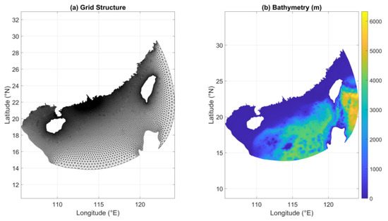
Figure 2.
Unstructured triangular grid and bathymetry of the SWAN model domain: (a) grid structure used in the SWAN model setup; (b) bathymetry of the study area, based on the unstructured mesh.
Wind-wave growth was represented using the WAM Cycle-4 (Janssen) formulation, in which the air–sea momentum flux is internally computed from the 10 m wind field, rather than prescribed through a fixed drag coefficient. Whitecapping dissipation was parameterized with the default SWAN coefficients. The SWAN model applied in this study was version 41.45. A computational time step of 10 min was adopted to balance accuracy and efficiency, with model outputs stored at hourly intervals. Preliminary sensitivity tests with a shorter time step (5 min) showed negligible improvement in significant wave height simulations, while substantially increasing computational cost. In addition, the model performance was evaluated against buoy observations. Although no further calibration of SWAN source-term coefficients was performed, the default parameterization provided reasonable agreement for the present application.
2.2.3. Model Validation
To evaluate the accuracy of the SWAN model when driven by ERA5 wind fields, the simulation of Super Typhoon Mangkhut (2018, International ID: 1822) and Kai-tak (2012, International ID: 1213) were conducted. The best track of the storms are illustrated in Figure 1. Mangkhut and Kai-tak were selected due to their extreme intensity and direct impact on the northern South China Sea, particularly the Pearl River Estuary. The primary aim of this validation is to assess whether ERA5 reanalysis datasets are capable of producing reliable wave hindcasts in this region, under typhoon conditions. The model running time spanned from 0000 UTC on 14 September to 2300 UTC on 17 September 2018, covering the evolution of Mangkhut within the computational domain.
Model performance was evaluated for two physical parameters: wind speed and significant wave height (Hs). Simulated results were compared against in situ observations from four buoy sites, QF303, QF304, QF306, and QF307, as introduced in Figure 1. Three evaluation metrics were used to quantify model accuracy: mean absolute error (MAE), root mean square error (RMSE) and the Pearson correlation coefficient (COR), which are defined in Equations (4)–(6). RMSE provides an absolute measure of deviation between simulated results (Mod) and observed values (Obs), while COR reflects the strength of linear agreement.
where N is the total number of data points, and and are the mean values of the modeled and observed data, respectively. A smaller RMSE and a higher COR indicate better model performance.
Figure 3 and Figure 4 show the validation results of wind speed and significant wave height at the four buoy stations, while Table 1 presents the corresponding error metrics. At QF304, QF306, and QF307 during Mangkhut (Figure 3a–c), the SWAN wind fields generally follow the observed trends, but slightly underestimate peak wind speeds, especially around the 20–30 h mark. At QF306 during Kai-tak (Figure 3d), the model captures the timing and magnitude of the peak reasonably well, though some early-phase overestimation (10–30 h) is visible. During Mangkhut (Figure 4a–c), SWAN generally reproduces the temporal evolution and peak Hs well at QF303, QF306, and QF307, with slight underestimation at peaks, especially at QF306. In Kai-tak (Figure 4d), the model successfully captures the sharp rise and fall in Hs at QF306, but appears to lag slightly behind observations in peak timing. Overall, these results demonstrate that SWAN provides a reasonably accurate representation of both wind forcing and wave evolution under typhoon conditions. This validation supports the use of SWAN-simulated wind and wave fields as reliable input for subsequent machine learning-based forecasting using RF and LSTM models.

Figure 3.
Comparison of observed and SWAN-simulated wind speed during Typhoons Mangkhut (2018) and Kai-tak (2012).
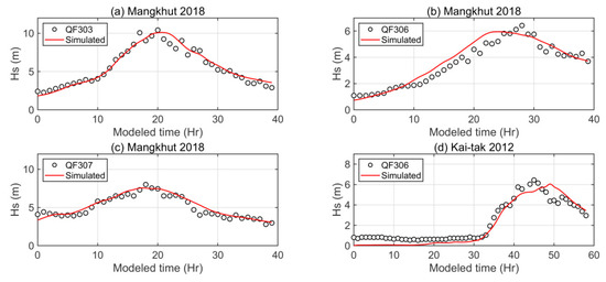
Figure 4.
Comparison of observed and SWAN-simulated significant wave height during Typhoons Mangkhut (2018) and Kai-tak (2012).

Table 1.
Validation statistics of 10 m wind speed and significant wave height at four buoy stations during Typhoon Mangkhut (2018) and Kai-tak (2012).
2.3. Machine Learning Models
To enable efficient wave forecasting beyond the computational limitations of physics-based SWAN simulations, two machine learning models were employed: Random Forest (RF) and Long Short-Term Memory (LSTM) neural networks. Trained on wind–wave time series derived from the SWAN model, these models serve as fast, data-driven surrogates for wave prediction.
2.3.1. Random Forest Model
Random Forest (RF) is a widely used ensemble learning algorithm based on decision trees, introduced by Leo Breiman [45]. It constructs a collection of trees trained on different subsets of the data, and aggregates their predictions to improve generalization and reduce overfitting. Owing to its robustness against noise and ability to capture nonlinear and partially random patterns, RF is suited for short-term prediction, which involves both deterministic and stochastic processes [19,46].
In this study, the RF model was trained to predict Hs using past wind speed and SWAN-simulated significant wave heights. The input features consisted of 6 h sequences of these, extracted from SWAN-simulated time series. The prediction targets were the Hs values at lead times of 3 and 6 h, respectively. Prior to model training, the original dataset was preprocessed by removing outliers and filling missing values, using linear interpolation. No z-score standardization was applied to the input features. This is because tree-based algorithms split the feature space based on threshold comparisons, and are invariant to monotonic transformations of individual features. Consequently, scaling the inputs does not alter the tree structures or the resulting predictions. Each time-series sample was constructed as a feature vector representing the past 6 h. Model evaluation followed an event-based split: 10 typhoon events were held out entirely as the independent test set, while the remaining 77 typhoon events were each randomly divided into 80% training and 20% validation subsets (Shown in Figure 5). The number of trees and maximum tree depth were optimized through a grid search to balance model complexity and generalization ability. The final model used 100 decision trees, with a maximum depth of 3. Model accuracy was evaluated on the testing set using RMSE, as defined in Equation (5).
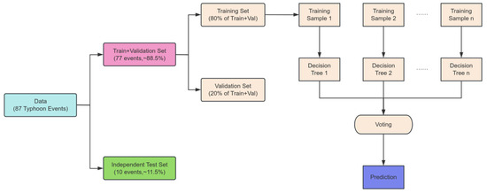
Figure 5.
Random forest model architecture for ensemble learning.
2.3.2. LSTM
Long Short-Term Memory (LSTM) networks are a type of recurrent neural network (RNN) specifically designed to learn long-range dependencies in sequential data. By incorporating gating mechanisms, including input, forget, and output gates, LSTM networks can effectively predict Hs [47,48].
In this study, an LSTM model was constructed to predict Hs based on time series inputs of wind and wave conditions. The input to the network is a 6-step sequence composed of 3 features at each time step: significant wave height, eastern wind speed, and northern wind speed. This results in a 6 × 3 feature matrix for each sample, constructed using a sliding-window approach. The network architecture consists of a single LSTM layer with 100 hidden units, followed by two fully connected layers. The first dense layer has 50 neurons with ReLU activation, and the second layer outputs a scalar representing the predicted Hs at a lead time of either 3 or 6 h. Only the final output of the LSTM sequence is used for regression. The structure of the LSTM network is illustrated in Figure 6. Prior to training, both input features and target values were normalized using z-score standardization. The model was trained using the Adam optimizer with an initial learning rate of 0.005, a batch size of 32, and a maximum of 50 epochs. A gradient clipping threshold of 1.0 was applied to prevent gradient explosion. The learning rate was reduced by 80% every 30 epochs, and data were shuffled before each epoch to enhance generalization. The key hyperparameters and training parameters used in the LSTM model are summarized in Table 2.
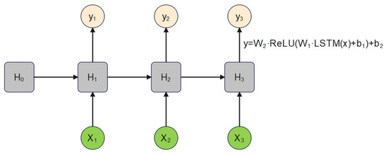
Figure 6.
Architecture of the LSTM network used for time-series prediction: x is input data, y is output data, H is hidden state.
Table 2.
Hyperparameters and training configuration of the LSTM model.
2.3.3. Experimental Design
To evaluate the performance of the two machine learning approaches (RF and LSTM) in significant wave height forecasting, four experimental configurations were designed by combining two modeling algorithms with two prediction lead times (3 h and 6 h). The selection of 3 h and 6 h forecast horizons was motivated by both operational and scientific considerations. Very short lead times (such as 1 h) provide limited added value over direct nowcasting, as real-time wave data or numerical model outputs are often already available within this interval. In contrast, longer horizons (such as 12 h) are prone to rapidly increasing uncertainty under highly dynamic typhoon conditions, particularly when future wind-field inputs are not provided. Lu et al. [28]’s study has also highlighted the practicality of 3 to 6 h forecasts.
All experiments used time-series data generated from SWAN simulations driven by historical typhoon wind fields by ERA5. To ensure strict independence between training and evaluation, the 87 historical typhoon events were divided such that 77 events were used in the training phase (with an internal 80:20 split for training and validation), and the remaining 10 events were reserved as an independent test set. The input features consisted of significant wave height (Hs), the u-component of wind speed (UWND), and the v-component of wind speed (VWND) over the preceding 6 h at each buoy location. The prediction target was the significant wave height at either a 3 h or 6 h lead time. A summary of the experimental setups is provided in Table 3.
Table 3.
Description of the four machine learning prediction schemes.
To quantitatively evaluate model performance across experiments, two statistical metrics were used: root mean square error (RMSE) and coefficient of determination (R2). RMSE has been defined previously in Equation (5). The coefficient of determination is calculated as
where and denote the observed and predicted values, respectively, and is the mean of the observed data. The value of R2 ranges between 0 and 1, with higher values indicating better agreement between predicted and observed results. Together with RMSE, these metrics were used to comprehensively assess model accuracy and generalization. The overall workflow of the prediction framework is illustrated in Figure 7.
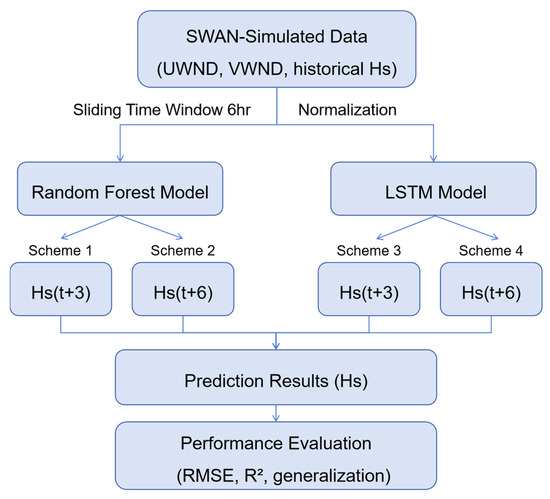
Figure 7.
The overall workflow of the prediction framework using SWAN-simulated data and two machine learning models.
In this study, we used the UWND and VWND as primary meteorological inputs, along with Hs. These two wind components were chosen because (i) they are the fundamental vector components from which wind magnitude and direction can be accurately derived, thereby implicitly incorporating directional effects without introducing redundant variables; (ii) in the offshore waters adjacent to the Pearl River Estuary, particularly under typhoon conditions, wind stress is the dominant physical forcing for wave growth, and these two components directly represent both magnitude and direction; (iii) they are directly available from ERA5 reanalysis data with high spatial and temporal resolution; and (iv) previous studies have demonstrated their strong predictive power for wave height forecasting in both statistical and machine learning frameworks [28].
3. Results
To ensure a consistent and fair evaluation of forecasting performance, the dataset included 10 typhoon events reserved for testing. Among these, six representative events—Gordon (1989), Brendan (1991), Kalmaegi (2014), Khanun (2017), Nesat (2022), and Koinu (2023)—were randomly selected for detailed presentation in this section. These events span a broad temporal range and capture diverse storm intensities and wave field evolutions in the northern South China Sea. Model performance was assessed separately for 3 h and 6 h forecast horizons (Section 3.1, Section 3.2 and Section 3.3). The spatial-generalization analysis in Section 3.4 was conducted using the 3 h forecast models only, as this lead time showed better accuracy and stability. The remaining four test events exhibited similar patterns, and are therefore not discussed in depth, to maintain conciseness.
3.1. The 3 h Wave-Height Forecast Performance of RF and LSTM
Figure 8 and Table 4 present the 3 h Hs forecast performance of the RF and LSTM models for six representative typhoon events at buoy QF-303. Across all events, the LSTM model consistently achieved lower RMSE values (average 0.233 m) and higher R2 values (average 0.953) than the RF model (average RMSE 0.271 m, R2 0.935), indicating better overall fitting accuracy and predictive capability. Event-specific results show that LSTM outperformed RF in five of the six typhoons in terms of RMSE, with notable improvements in high-variability events such as Kalmaegi 2014 (RMSE reduced from 0.21 m to 0.17 m) and Koinu 2023 (0.25 m to 0.20 m). Even in earlier events like Gordon 1989, LSTM reduced the error by 0.08 m, while maintaining high R2 (>0.97). The only event where LSTM’s RMSE slightly exceeded RF’s was Khanun 2017 (0.25 m vs. 0.23 m), which coincided with a relatively smooth peak evolution where RF’s tree-based structure captured the wave growth/decay adequately.
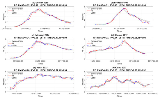
Figure 8.
Comparison of significant wav- height time series at 3 h forecast horizons. The black circles represent SWAN results at Buoy QF303. The red solid line indicates predictions from the RF model, while the blue dashed line shows predictions from the LSTM model.
Table 4.
Performance metrics (RMSE and R2) of 3 h significant wave height forecasts for each typhoon event and overall average.
For the 3 h forecast at buoy QF-303, both RF and LSTM models showed good agreement with SWAN-simulated peak significant wave heights (Hs) across the all test typhoon events (Table 5). The mean absolute percentage error (MAPE) for peak Hs was 6.71% for RF and 4.54% for LSTM, indicating that the LSTM model consistently provided slightly more accurate peak estimates. In terms of temporal alignment, lag times between the predicted and SWAN reference peaks varied across events. RF predictions showed a mean lag of 2.17 h, with some events (such as Kalmaegi 2014) producing early peaks (−2 h). LSTM lag times were generally shorter, averaging 0.5 h, and in several events (such as Khanun 2017 and Nesat 2022) the predicted peaks were synchronized with SWAN results. These findings suggest that, for QF-303, the LSTM model not only achieves higher accuracy in peak wave-height estimation, but also reduces peak timing errors compared to the RF model. LSTM exhibited a stronger ability to capture temporal dynamics. This may be attributed to the LSTM’s gated structure, which effectively captures long-term dependencies between wind forcing and wave response, enhancing its responsiveness under nonlinear and high-variability conditions. Its advantage in fitting extremes and handling complex typhoon-induced wave fields suggests that LSTM is more suitable for short-term forecasting of significant wave heights under extreme weather scenarios.
Table 5.
QF 303 peak significant wave heights (Hs) from SWAN model, RF, and LSTM models for test typhoon events, with percentage errors and lag times (3 h forecast horizons).
3.2. The 6 h Wave-Height Forcast Performance of RF and LSTM
To assess the sensitivity of model performance to forecast lead time, we extended the comparison between RF and LSTM models to a 6 h prediction horizon. Figure 9 shows the time-series predictions from both models during the six representive typhoon events referenced against SWAN-simulated results at buoy QF303. The associated RMSE and R2 values are annotated in Figure 9 and summarized in Table 6.
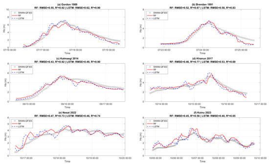
Figure 9.
Comparison of significant wave-height time series at 6 h forecast horizons. The black circles represent SWAN results at Buoy QF303. The red solid line indicates predictions from the RF model, while the blue dashed line shows predictions from the LSTM model.
Table 6.
Performance metrics (RMSE and R2) of 6-hour significant wave height forecasts for each typhoon event, and overall average.
Compared to the 3 h forecast, both models exhibited a notable drop in prediction accuracy in Table 6. RF achieved a mean RMSE of 0.480 m and R2 of 0.795, while LSTM yielded a slightly higher RMSE of 0.513 m and a lower R2 of 0.785. These values represented increases in average error, indicating that longer forecast horizons led to amplified uncertainty and cumulative errors. In terms of event-specific performance, RF achieved lower RMSEs in events such as Gordon, Kalmaegi, and Nesat. For example, in Gordon (1989), RF attained an RMSE of 0.55 m, marginally outperforming LSTM’s 0.62 m. Similarly, in Kalmaegi (2014), the RMSEs were 0.43 m (RF) and 0.49 m (LSTM). However, in the Koinu (2023) simulation, LSTM showed superior performance, reducing the RMSE from 0.45 m (RF) to 0.40 m, which reflected its capacity to track complex, multi-peaked wave patterns. Figure 9 also illustrates the fact that both models performed well during stable wave conditions, but their accuracy degraded near peaks or turning points. RF tended to show delayed decay or early drop-off, while LSTM exhibited localized overfitting or oscillations, especially during Brendan and Khanun, where sharp changes led to discontinuous predictions. These findings suggested that although LSTM possessed inherent advantages in modeling nonlinear dynamics, the lack of future wind field input in current settings constrained its long-range forecasting capability.
For the 6 h forecast horizon at buoy QF-303, both RF and LSTM models reproduced the general magnitude of SWAN-simulated peak significant wave heights (Hs) (shown in Table 7). The MAPE for peak Hs was 10.13% for RF and 12.34% for LSTM, indicating that RF yielded slightly more accurate peak magnitude estimates at this longer lead time. Peak-timing errors were also more pronounced: the mean absolute lag time was 1.17 h for RF and 1.33 h for LSTM. RF predictions tended to be delayed by 1–2 h in several events (such as Gordon 1989, Khanun 2017, and Nesat 2022) but occurred earlier by 1–2 h in others. LSTM exhibited a similar pattern, but with larger early-peak deviations in some events (up to 3 h early for Koinu 2023). Despite the overall decline in performance at 6 h horizons, this analysis provided a necessary baseline for understanding the temporal limits of data-driven models under typhoon-induced conditions. The results revealed that RF maintained smoother and more stable outputs, on average, while LSTM retained potential advantages in capturing extremes.
Table 7.
QF 303 peak significant wave heights (Hs) from SWAN model, RF, and LSTM models for test typhoon events, with percentage errors and lag times (6 h forecast horizons).
3.3. Performance Comparison Between 3 h and 6 h Forecasts
Figure 10 compares the 3 h and 6 h forecast performances of the RF and LSTM models at buoy QF-303. Across all typhoon events, both models showed increased RMSE and reduced R2 when the forecast horizon was extended, indicating a degradation in predictive accuracy over longer lead times. Interestingly, typhoon events with relatively smaller increases in RMSE, such as Nesat (2022) and Koinu (2023), exhibited some of the largest reductions in R2. This pattern suggests that even when the magnitude error remains relatively stable, the temporal correlation between predicted and reference wave-height series can degrade markedly. In certain storm events, extending the forecast horizon has a stronger impact on phase alignment and predictive consistency than on absolute error magnitude.
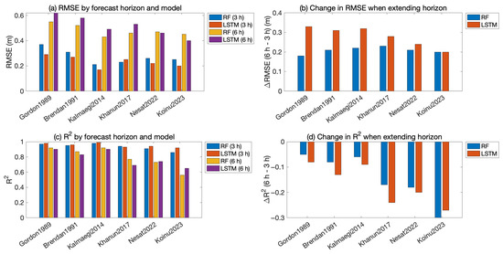
Figure 10.
Performance comparison between 3 h and 6 h forecasts for RF and LSTM models at buoy QF-303: (a) RMSE values; (b) change in RMSE when extending the forecast horizon from 3 h to 6 h; (c) R2 values; (d) change in R2 when extending the forecast horizon from 3 h to 6 h.
Figure 11 illustrated the variations in peak significant wave-height (Hs) prediction errors and peak timing differences between the 3 h and 6 h forecasts for the six representative typhoon events. For peak Hs magnitude, both RF and LSTM models exhibited increased MAPE when the forecast horizon was extended to 6 h, indicating reduced accuracy in capturing extremes at longer lead times. In the 3 h forecasts, LSTM consistently achieved lower MAPE values than RF, reflecting its advantage in short-term peak estimation. However, for the 6 h forecasts, the LSTM errors increased more sharply in some events (such as Nesat (2022) and Koinu (2023)), suggesting greater sensitivity to the loss of recent temporal information. In peak timing, RF tended to delay peaks by 2–3 h in some events, while LSTM showed smaller lags at 3 h but produced early peaks (up to 3 h) in some 6 h forecasts. Overall, LSTM excels in short-term peak prediction, whereas RF yields more stable—but often delayed—timing at longer horizons.
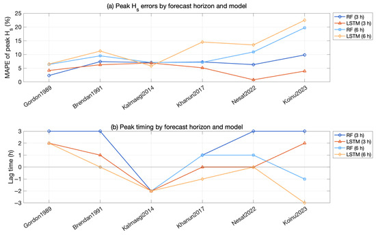
Figure 11.
Peak significant wave-height errors (MAPE) and peak timing differences (lag times) for RF and LSTM models at 3 h and 6 h forecast horizons across six typhoon events.
3.4. Spatial Generalization of 3 h Forecast Models to Other Locations
To assess the spatial-generalization capability of the trained models, the RF and LSTM models, originally developed at buoy QF-303 for 3 h forecast horizons, were applied to three sites: QF306, QF307 and QF308 (center of the typhoon selection zone). QF-304 was excluded from this analysis, as it lies outside the typhoon selection zone defined in Section 2.1.
Both models demonstrated strong generalization ability across the three sites in Table 8. The LSTM model consistently outperformed the RF model, achieving lower RMSE and higher R2 across all locations. Specifically, at QF306, LSTM achieved an RMSE of 0.283 m and an R2 of 0.974, clearly better than RF’s RMSE of 0.397 m and R2 of 0.949. At QF307, performance improved further for both models, with LSTM yielding an RMSE of 0.234 m and an R2 of 0.950. At QF308, the LSTM model still achieved an RMSE of 0.286 m and an R2 of 0.975, while RF recorded an RMSE of 0.417 m and an R2 of 0.947. These results demonstrate that both models are capable of transferring learned wind–wave relationships from the training site (QF303) to other nearby locations, but LSTM exhibits stronger robustness and stability. Interestingly, the spatial location of the target sites relative to the training site (QF303) appears to influence model performance. QF306 and QF308 are both located to the west of QF303 (Figure 1), and their R2 are not only similar to each other, but also noticeably better than those for QF307, which is situated to the east of QF303. This difference may be attributed to the prevailing typhoon tracks and associated wave propagation patterns in the northern South China Sea, where sites on the same side of the training buoy are more likely to share similar wind–wave dynamics, thereby benefiting model transferability.
Table 8.
Averaged performance metrics (RMSE and R2) of 3 h significant wave-height forecasts for all 87 typhoon events at QF306, QF307, and QF308, using RF and LSTM models trained at QF303.
Detailed time-series comparisons for six representative typhoon events at each site are presented in Figure 12, Figure 13 and Figure 14. Despite being trained solely on QF303 data, the models were able to reproduce the temporal evolution of wave height under different typhoon paths and spatial conditions. Both models captured the rising and falling trends of wave height reasonably well. In particular, for events such as Kalmaegi and Nesat, the LSTM model displayed a high level of temporal consistency with the reference curves, demonstrating its capacity to generalize the underlying wind–wave dynamics beyond the training site.
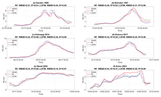
Figure 12.
Comparison of significant wave-height time series at 3 h forecast horizons at Buoy QF306.
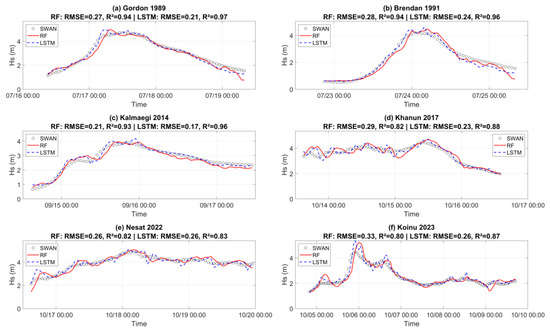
Figure 13.
Comparison of significant wave-height time series at 3 h forecast horizons at Buoy QF307.
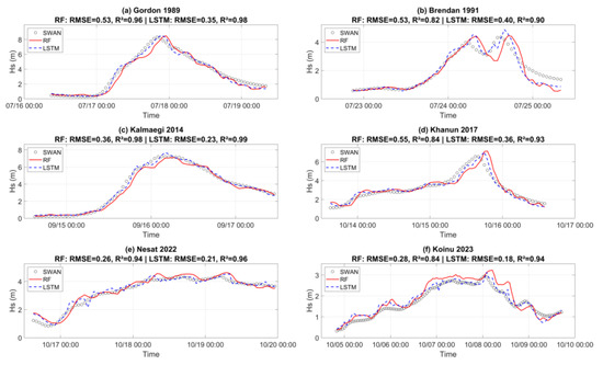
Figure 14.
Comparison of significant wave-height time series at 3 h forecast horizons at Buoy QF308.
4. Discussion
This study developed and evaluated RF and LSTM for predicting Hs under typhoon conditions in the PRE region. SWAN-simulated data from 87 historical typhoon events were used, with 77 events for model training and 10 independent events for validation, enabling assessment of both event-level and spatial-generalization performance.
Our results indicate that RF tends to maintain higher stability during the early development and late dissipation stages of typhoon-induced waves, whereas LSTM performs better near the peak stage, when wave growth is most rapid. This stage-dependent behavior reflects the different learning mechanisms of the two models: RF excels at capturing relatively stable patterns with less temporal dependence, while LSTM is better suited for modeling highly dynamic transitions. These findings are consistent with previous literature that highlights the effectiveness of deep learning in capturing highly dynamic wave processes [38]. Moreover, regarding forecast horizons, the reduced accuracy in the 6 h predictions compared to the 3 h predictions is likely due to the absence of future wind-field inputs, which limits the models ability to capture subsequent changes in wave growth and decay. This effect is more pronounced in LSTM, which relies heavily on recent temporal patterns that may lose predictive relevance over longer horizons.
Although model performance across all validation typhoon events was broadly similar, certain variations were observed. For instance, during Typhoon Koinu 2023, the spatial-generalization performance at QF306 was notably lower than at QF307, despite both sites being geographically close (shown in Figure 12f and Figure 13f). A likely contributing factor is the relative position of the typhoon center in relation to the prediction site, which can strongly influence the local wind–wave generation environment. This variable was not explicitly included in the present study, meaning that spatial differences in storm forcing may not have been fully captured by the models. A similar perspective was emphasized by [49], who highlighted the importance of incorporating spatially varying wind fields for improving wave forecasts. Future work could therefore explore adding the relative distance and orientation between the typhoon center and prediction sites, as additional input features, to enhance model robustness in cross-event applications. Moreover, our findings highlight the concerns raised by [50] that ML models trained on historical data may perform unsatisfactorily when applied to newer data, due to shifting atmospheric and oceanic conditions. Future studies may mitigate these limitations by incorporating additional and more recent datasets, or by adopting physics-informed machine learning frameworks that embed governing wave dynamics into the predictive process.
5. Conclusions
In this paper, for the typhoon-prone offshore regions of the Pearl River Estuary, 3 h forecasts consistently outperformed 6 h forecasts, with LSTM surpassing RF at shorter lead times but experiencing a steeper accuracy decline as the horizon extended. By coupling high-resolution numerical simulations with machine learning, the proposed framework delivers rapid and accurate wave forecasts in a region where in situ observations are sparse but the economic stakes are high. This approach offers a transferable solution for short-term wave forecasting in other data-scarce yet high-risk coastal environments, and provides a practical pathway for enhancing real-time hazard preparedness.
Author Contributions
Conceptualization, M.M. and S.X.; methodology, M.M.; software, G.C.; validation, M.M. and G.C.; formal analysis, M.M.; investigation, W.T. and K.Y.; resources, M.M.; data curation, G.C.; writing—original draft preparation, M.M.; writing—review and editing, M.M. and W.T.; visualization, M.M.; supervision, S.X.; project administration, S.X.; funding acquisition, S.X. and K.Y. All authors have read and agreed to the published version of the manuscript.
Funding
This study was funded by the National Natural Science Foundation of China [Grant Numbers 52271266, 52471274].
Data Availability Statement
The raw data supporting the conclusions of this article will be made available by the authors on request.
Conflicts of Interest
The authors declare no conflicts of interest.
Abbreviations
The following abbreviations are used in this manuscript:
| Hs | Significant wave height (m) |
| SWAN | Simulating Waves Nearshore Model |
| ML | Machine Learning |
| SVMs | Support Vector Machines |
| RF | Random Forest |
| LSTM | Long Short-Term Memory Networks |
| PRE | Pearl River Estuary |
| ECMWF | European Centre for Medium-Range Weather Forecasts |
| SCSB-SOA | South China Sea Branch of the State Oceanic Administration |
| MAE | Mean absolute error |
| RMSE | Root mean square error |
| COR | Pearson correlation coefficient |
| R2 | Coefficient of determination |
| UWND | U-component of wind speed (m/s) |
| VWND | V-component of wind speed (m/s) |
| MAPE | Mean absolute percentage error (%) |
Appendix A
Table A1.
List of 87 historical typhoon events (names and IDs) used in this paper.
Table A1.
List of 87 historical typhoon events (names and IDs) used in this paper.
| Serial Number | Typhoon Number and Name | Serial Number | Typhoon Number and Name | Serial Number | Typhoon Number and Name |
|---|---|---|---|---|---|
| 1 | 202304Talim | 30 | 200107Yutu | 59 | 198721Nina |
| 2 | 202309Saola | 31 | 200104Utor | 60 | 198607Peggy |
| 3 | 202314Koinu | 32 | 200016Wukong | 61 | 198621Ellen |
| 4 | 202220Nesat | 33 | 199910York | 62 | 198515Tess |
| 5 | 202222Nalgae | 34 | 199908Sam | 63 | 198504Hal |
| 6 | 201822Mangkhut | 35 | 199903Maggie | 64 | 198314Joe |
| 7 | 201720Khanun | 36 | 199902Leo | 65 | 198309Ellen |
| 8 | 201713Hato | 37 | 199914Dan | 66 | 198103Ike |
| 9 | 201604Nida | 38 | 199810Babs | 67 | 198116Clara |
| 10 | 201622Haima | 39 | 199710Victor | 68 | 198007Joe |
| 11 | 201522Mujigae | 40 | 199615Sally | 69 | 197908Hope |
| 12 | 201510Linfa | 41 | 199515Sibyl | 70 | 197801Olive |
| 13 | 201415Kalmaegi | 42 | 199514Ryan | 71 | 197609Iris |
| 14 | 201311Utor | 43 | 199509Kent | 72 | 197515Flossie |
| 15 | 201319Usagi | 44 | 199505Helen | 73 | 197514Elsie |
| 16 | 201329Krosa | 45 | 199504Gary | 74 | 197411Ivy |
| 17 | 201208Vicente | 46 | 199309Tasha | 75 | 197424Elaine |
| 18 | 201214Tembin | 47 | 199302Koryn | 76 | 197422Carmen |
| 19 | 201213Kai-tak | 48 | 199318Dot | 77 | 197421Bess |
| 20 | 200906Molave | 49 | 199316Becky | 78 | 197313Louise |
| 21 | 200903Linfa | 50 | 199315Abe | 79 | 197307Georgia |
| 22 | 200915Koppu | 51 | 199111Fred | 80 | 197304Dot |
| 23 | 200812Niru | 52 | 199108Brendan | 81 | 197118Rose |
| 24 | 200814Hagupit | 53 | 199107Amy | 82 | 197114Lucy |
| 25 | 200606Prapiroon | 54 | 199006Percy | 83 | 197108Freda |
| 26 | 200510Sanvu | 55 | 199003Marian | 84 | 197125Della |
| 27 | 200312Krovanh | 56 | 198908Gordon | 85 | 197012Iris |
| 28 | 200307Imbudo | 57 | 198903Brenda | 86 | 197011Georgia |
| 29 | 200313Dujuan | 58 | 198805Warren | 87 | 196903Viola |
Note: Bold typhoons indicate events used for independent test set of the machine learning models. Italic typhoons indicate events used for validation of the SWAN model.
References
- Abouhalima, M.; das Neves, L.; Taveira-Pinto, F.; Rosa-Santos, P. Machine learning in coastal engineering: Applications, challenges, and perspectives. J. Mar. Sci. Eng. 2024, 12, 638. [Google Scholar] [CrossRef]
- Afzal, M.S.; Kumar, L.; Chugh, V.; Kumar, Y.; Zuhair, M. Prediction of significant wave height using machine learning and its application to extreme wave analysis. J. Earth Syst. Sci. 2023, 132, 51. [Google Scholar] [CrossRef]
- Tamizi, A.; Alves, J.-H.; Young, I.R. The physics of ocean wave evolution within tropical cyclones. J. Phys. Oceanogr. 2021, 51, 2373–2388. [Google Scholar] [CrossRef]
- Thomas, T.J.; Dwarakish, G. Numerical wave modelling—A review. Aquat. Procedia 2015, 4, 443–448. [Google Scholar] [CrossRef]
- Booij, N.; Holthuijsen, L.H.; Ris, R.C. The “SWAN” wave model for shallow water. In Proceedings of the 25th International Conference on Coastal Engineering, Orlando, FL, USA, 2–6 September 1996; pp. 668–676. [Google Scholar] [CrossRef]
- DHI. MIKE 21 Flow Model FM, Hydrodynamic Module, User Guide; DHI Technologies: Maharashtra, India, 2021. [Google Scholar]
- Deltares. Delft3D-FM, D-FLOW Flexible Mesh, User Manual; Deltares Delft: Delft, The Netherlands, 2021. [Google Scholar]
- Zhao, H.; Chen, P.; Zhang, W.; Yan, S.; Yang, J.; Kong, J. On the capability of SWAN model for South Atlantic Ocean wave simulation. Ocean. Dyn. 2025, 75, 51. [Google Scholar] [CrossRef]
- Huang, Y.; Weisberg, R.H.; Zheng, L.; Zijlema, M. Gulf of Mexico hurricane wave simulations using SWAN: Bulk formula-based drag coefficient sensitivity for Hurricane Ike. J. Geophys. Res. Oceans 2013, 118, 3916–3938. [Google Scholar] [CrossRef]
- Ou, S.-H.; Liau, J.-M.; Hsu, T.-W.; Tzang, S.-Y. Simulating typhoon waves by SWAN wave model in coastal waters of Taiwan. Ocean Eng. 2002, 29, 947–971. [Google Scholar] [CrossRef]
- Xie, W.; Xu, G.; Zhang, H.; Dong, C. Developing a deep learning-based storm surge forecasting model. Ocean Model. 2023, 182, 102179. [Google Scholar] [CrossRef]
- Serras, P.; Ibarra-Berastegi, G.; Sáenz, J.; Ulazia, A. Combining random forests and physics-based models to forecast the electricity generated by ocean waves: A case study of the Mutriku wave farm. Ocean Eng. 2019, 189, 106314. [Google Scholar] [CrossRef]
- Di Bacco, M.; Contento, A.; Scorzini, A.R. Exploring the compound nature of coastal flooding by tropical cyclones: A machine learning framework. J. Hydrol. 2024, 645, 132262. [Google Scholar] [CrossRef]
- Kim, T.; Lee, W.-D. Review on applications of machine learning in coastal and ocean engineering. J. Ocean Eng. Technol. 2022, 36, 194–210. [Google Scholar] [CrossRef]
- Masria, A.; Abouelsaad, O. Artificial intelligence applications in coastal engineering and its challenges—A review. Cont. Shelf Res. 2025, 286, 105425. [Google Scholar] [CrossRef]
- James, S.C.; Zhang, Y.; O’DOnncha, F. A machine learning framework to forecast wave conditions. Coast. Eng. 2018, 137, 1–10. [Google Scholar] [CrossRef]
- Jiang, J.; Huang, Z.-G.; Grebogi, C.; Lai, Y.-C. Predicting extreme events from data using deep machine learning: When and where. Phys. Rev. Res. 2022, 4, 023028. [Google Scholar] [CrossRef]
- Jing, Y.; Zhang, L.; Hao, W.; Huang, L. Numerical study of a CNN-based model for regional wave prediction. Ocean Eng. 2022, 255, 111400. [Google Scholar] [CrossRef]
- Campos, R.M.; Costa, M.O.; Almeida, F.; Soares, C.G. Operational wave forecast selection in the Atlantic Ocean using random forests. J. Mar. Sci. Eng. 2021, 9, 298. [Google Scholar] [CrossRef]
- Berbić, J.; Ocvirk, E.; Carević, D.; Lončar, G. Application of neural networks and support vector machine for significant wave height prediction. Oceanologia 2017, 59, 331–349. [Google Scholar] [CrossRef]
- Mahjoobi, J.; Mosabbeb, E.A. Prediction of significant wave height using regressive support vector machines. Ocean Eng. 2009, 36, 339–347. [Google Scholar] [CrossRef]
- Demetriou, D.; Michailides, C.; Papanastasiou, G.; Onoufriou, T. Nowcasting significant wave height by hierarchical machine learning classification. Ocean Eng. 2021, 242, 110130. [Google Scholar] [CrossRef]
- Wei, Z. Forecasting wind waves in the US Atlantic Coast using an artificial neural network model: Towards an AI-based storm forecast system. Ocean Eng. 2021, 237, 109646. [Google Scholar] [CrossRef]
- Patanè, L.; Iuppa, C.; Faraci, C.; Xibilia, M.G. A deep hybrid network for significant wave height estimation. Ocean Model. 2024, 189, 102363. [Google Scholar] [CrossRef]
- Duong, N.T.; Tran, K.Q.; Luu, L.X.; Tran, L.H. Prediction of breaking wave height by using artificial neural network-based approach. Ocean Model. 2023, 182, 102177. [Google Scholar] [CrossRef]
- Kang, D.; Oh, S. A Study of Machine Learning Model for Prediction of Swelling Waves Occurrence on East Sea. J. Korean Inst. Inf. Technol. 2019, 17, 11–17. [Google Scholar] [CrossRef]
- Jörges, C.; Berkenbrink, C.; Stumpe, B. Prediction and reconstruction of ocean wave heights based on bathymetric data using LSTM neural networks. Ocean Eng. 2021, 232, 109046. [Google Scholar] [CrossRef]
- Lu, X.; Peng, Z.; Li, C.; Chen, L.; Qiao, G.; Li, C.; Yang, B.; He, Q. An innovative deep learning model for accurate wave height predictions with enhanced performance for extreme waves. Ocean Eng. 2025, 322, 120502. [Google Scholar] [CrossRef]
- Tan, W.; Yuan, C.; Xu, S.; Xu, Y.; Stocchino, A. A Swin-Transformer-based deep-learning model for rolled-out predictions of regional wind waves. Phys. Fluids 2025, 37, 036625. [Google Scholar] [CrossRef]
- Huang, L.; Jing, Y.; Chen, H.; Zhang, L.; Liu, Y. A regional wind wave prediction surrogate model based on CNN deep learning network. Appl. Ocean Res. 2022, 126, 103287. [Google Scholar] [CrossRef]
- Zhang, J.; Luo, F.; Quan, X.; Wang, Y.; Shi, J.; Shen, C.; Zhang, C. Improving wave height prediction accuracy with deep learning. Ocean Model. 2024, 188, 102312. [Google Scholar] [CrossRef]
- Ho, C.-Y.; Cheng, K.-S.; Ang, C.-H. Utilizing the random forest method for short-term wind speed forecasting in the coastal area of central Taiwan. Energies 2023, 16, 1374. [Google Scholar] [CrossRef]
- Zhang, W.; Sun, Y.; Wu, Y.; Dong, J.; Song, X.; Gao, Z.; Pang, R.; Guoan, B. A deep-learning real-time bias correction method for significant wave height forecasts in the Western North Pacific. Ocean Model. 2024, 187, 102289. [Google Scholar] [CrossRef]
- Sithara, S.; Unni, A.; Pramada, S. Machine learning approaches to predict significant wave height and assessment of model uncertainty. Ocean Eng. 2025, 328, 121039. [Google Scholar] [CrossRef]
- Bekiryazıcı, Ş.; Amarouche, K.; Ozcan, N.; Akpınar, A. An innovative deep learning-based approach for significant wave height forecasting. Ocean Eng. 2025, 323, 120623. [Google Scholar] [CrossRef]
- Hasan, A.; Kayes, I.; Alam, M.; Shahriar, T.; Habib, M.A. Generalized machine learning models to predict significant wave height utilizing wind and atmospheric parameters. Energy Convers. Manag. X 2024, 23, 100623. [Google Scholar] [CrossRef]
- O’dOnncha, F.; Zhang, Y.; Chen, B.; James, S.C. An integrated framework that combines machine learning and numerical models to improve wave-condition forecasts. J. Mar. Syst. 2018, 186, 29–36. [Google Scholar] [CrossRef]
- Wei, Z.; Davison, A. A convolutional neural network based model to predict nearshore waves and hydrodynamics. Coast. Eng. 2022, 171, 104044. [Google Scholar] [CrossRef]
- Chen, J.; Pillai, A.C.; Johanning, L.; Ashton, I. Using machine learning to derive spatial wave data: A case study for a marine energy site. Environ. Model. Softw. 2021, 142, 105066. [Google Scholar] [CrossRef]
- Chen, C.; Lin, H.; Guan, D.; Cai, F.; Wang, Q.; Liu, Q. Enhancing typhoon wave hindcasting with random forests and BP neural networks in the SWAN model. Front. Mar. Sci. 2024, 11, 1472047. [Google Scholar] [CrossRef]
- Hersbach, H.; Bell, B.; Berrisford, P.; Hirahara, S.; Horányi, A.; Muñoz-Sabater, J.; Nicolas, J.; Peubey, C.; Radu, R.; Schepers, D. The ERA5 global reanalysis. Q. J. R. Meteorol. Soc. 2020, 146, 1999–2049. [Google Scholar] [CrossRef]
- Elshinnawy, A.I.; Menéndez, M.; Medina, R. A parameterization for the correction of ERA5 severe winds for extreme ocean wave modelling. Ocean Eng. 2024, 312, 119048. [Google Scholar] [CrossRef]
- Amante, C.; Eakins, B.W. ETOPO1 Arc-Minute Global Relief Model: Procedures, Data Sources and Analysis; National Oceanic and Atmospheric Administration: Washington, DC, USA, 2009. [Google Scholar]
- SCSB-SOA. 2025. Available online: http://g.hyyb.org/systems/HyybData/DataDB/ (accessed on 1 January 2025).
- Breiman, L. Random forests. Mach. Learn. 2001, 45, 5–32. [Google Scholar] [CrossRef]
- Ibarra-Berastegi, G.; Saénz, J.; Esnaola, G.; Ezcurra, A.; Ulazia, A. Short-term forecasting of the wave energy flux: Analogues, random forests, and physics-based models. Ocean Eng. 2015, 104, 530–539. [Google Scholar] [CrossRef]
- Abdullah, F.A.R.; Ningsih, N.S.; Al-Khan, T.M. Significant wave height forecasting using long short-term memory neural network in Indonesian waters. J. Ocean Eng. Mar. Energy 2022, 8, 183–192. [Google Scholar] [CrossRef]
- Fan, S.; Xiao, N.; Dong, S. A novel model to predict significant wave height based on long short-term memory network. Ocean Eng. 2020, 205, 107298. [Google Scholar] [CrossRef]
- Chang, H.-K.; Liou, J.-C.; Liu, S.-J.; Liaw, S.-R. Simulated wave-driven ANN model for typhoon waves. Adv. Eng. Softw. 2011, 42, 25–34. [Google Scholar] [CrossRef]
- Ellenson, A.; Pei, Y.; Wilson, G.; Özkan-Haller, H.T.; Fern, X. An application of a machine learning algorithm to determine and describe error patterns within wave model output. Coast. Eng. 2020, 157, 103595. [Google Scholar] [CrossRef]
Disclaimer/Publisher’s Note: The statements, opinions and data contained in all publications are solely those of the individual author(s) and contributor(s) and not of MDPI and/or the editor(s). MDPI and/or the editor(s) disclaim responsibility for any injury to people or property resulting from any ideas, methods, instructions or products referred to in the content. |
© 2025 by the authors. Licensee MDPI, Basel, Switzerland. This article is an open access article distributed under the terms and conditions of the Creative Commons Attribution (CC BY) license (https://creativecommons.org/licenses/by/4.0/).