Faulted-Pole Discrimination in Shipboard DC Microgrids Using S-Transformation and Convolutional Neural Networks

Abstract

The complex topology of shipboard DC microgrids and the strong coupling between positive and negative poles during faults pose significant challenges for faulted-pole identification, especially under high-resistance conditions. To address these issues, this paper proposes a novel faulted-pole identification method based on S-Transformation and convolutional neural networks (CNNs). Single-ended voltage and current measurements from the generator side are used to generate time–frequency spectrograms via S-Transformation, which are then processed by a CNN trained to classify the faulted pole. This approach avoids reliance on complex threshold settings. Simulation results on a representative shipboard DC microgrid demonstrate that the proposed method achieves high accuracy, fast response, and strong robustness, even under high-resistance fault scenarios. The method significantly enhances the selectivity and reliability of fault protection, offering a promising solution for advanced marine DC power systems. Compared to conventional fault-diagnosis techniques, the proposed model achieves notable improvements in classification accuracy and computational efficiency for line-fault detection.

1. Introduction

Shipboard DC microgrids have emerged as a key technological direction in modern ship-power systems, offering higher system stability and significant reductions in space and weight compared to traditional shipboard AC systems. The use of power electronic devices in DC microgrids enables the elimination of large transformers, reduces cable weight, and allows for the stable parallel operation of generators with different frequencies, thus lowering fuel consumption and improving overall efficiency [1,2,3,4,5]. Despite recent advancements, protection and fault management in shipboard DC microgrids remain technically challenging.

The application of artificial intelligence (AI) techniques in fault protection for DC grids has been growing, particularly in fault early-warning, fault detection, and internal–external fault discrimination. Deep learning and semi-supervised learning have significantly enhanced fault-detection capabilities, but AI-based pole selection in DC grids remains underexplored. Traditional fault-pole identification methods face challenges in shipboard DC microgrids due to complex system topology and difficulty distinguishing high-impedance fault signals. To address these issues, this paper proposes a fault-pole discrimination method based on S-Transformation and CNN, which can accurately and quickly identify faults, especially in high-impedance fault scenarios.

The rest of the paper is organized as follows: Section 2 introduces a literature review in the relevant field; Section 3 introduces the principles of S-Transformation and CNNs; Section 4 presents the proposed faulted-pole discrimination model and its parameter settings; Section 5 evaluates the performance of the model through case studies and compares it with traditional methods; and Section 6 concludes the paper.

2. Literature Review

2.1. AI Applications in DC-Grid Fault Protection

Artificial intelligence techniques have seen growing use in DC grid protection and fault management, particularly for fault early-warning systems, fault detection, and internal–external fault discrimination.

AI techniques in fault early-warning systems involves their widespread application in predicting electrical machine faults. There is a particular focus on deep learning methods (such as autoencoders, Generative Adversarial Networks, and reinforcement learning) and semi-supervised learning to reduce reliance on labeled datasets, thereby significantly enhancing fault-detection capabilities, particularly in renewable energy systems [6]. In [7], an adversarial-based deep-transfer-learning model is proposed to detect and classify short-circuit faults in DC microgrids without using historical fault data. In [8], the reinforcement learning and convolutional neural network–long short-term memory (LSTM) model are used for fault diagnosis and protection strategy design in the DC grids. In [9], a fault-protection scheme based on Discrete Wavelet Transform (DWT) multi-resolution analysis, and Artificial Neural Networks (ANNs) is proposed for fault detection and classification in multi-terminal HVDC grids, which significantly improves fault-recognition accuracy and reduces computational burden. In [10], a voltage instability assessment method based on deep-transfer-learning convolutional neural networks (DTCNN) is proposed for post-fault voltage recovery and stability control in DC microgrids, which achieves efficient and real-time voltage monitoring and protection. In [11], a fault location method based on Support Vector Machines (SVMs) is proposed for high-impedance faults in DC microgrid clusters, with high accuracy, low cost, and no reliance on communication links. In [12], an online cascading-failure screening method based on Gradient Boosting Decision Tree (GBDT) and dynamic weighting techniques is proposed. The method is designed to quickly identify and predict high-risk cascading failures in the sending-end systems of Line-Commutated Converter High-Voltage Direct Current (LCC-HVDC) with high wind power penetration. In [13], a machine learning-based fault-detection and -location method for low-voltage DC microgrids is proposed by combining Compressed Sensing (CS) and Regression Tree (RT) techniques for fast fault detection and using a feature matrix with an LSTM model for high-accuracy fault localization. In [14], a fault-diagnosis method for HVDC systems based on LSTM networks and a knowledge graph is presented, to achieve high-precision and rapid fault classification by extracting fault waveform features. In [15], a fault-detection and classification method for low-voltage DC microgrids is proposed. The method combines novel morphological operators and a multi-class AdaBoost algorithm, efficiently denoising and accurately classifying AC and DC side faults, improving both fault-detection accuracy and response speed. In [16], a series arc fault-diagnosis method based on multi-scale features and random forests is proposed. The method accurately locates faults in DC distribution systems, meeting high accuracy and real-time performance requirements. In [17], a data-driven hybrid machine learning approach is proposed. The method achieves high-precision fault detection and classification in low-voltage DC microgrids, using a bagged ensemble learner and a cosine k-nearest neighbor algorithm. In [18], an online fault-protection method based on transfer-learning convolutional neural networks (TCNNs) is proposed for low-voltage DC microgrid systems, capable of accurately detecting and classifying faults, thus significantly improving accuracy and reducing data redundancy. Some studies have incorporated fault characteristics into AI-based methods, resulting in improved fault-detection accuracy over traditional protection schemes and shallow AI models, as well as enhanced interpretability and reduced computational complexity compared to deep learning-based approaches [19].

Despite these advances, AI-driven pole selection (i.e., determining whether a fault is on the positive pole, negative pole, or both) remains underexplored, creating a gap in comprehensive AI-based DC-grid protection.

2.2. Pole Selection Research in DC Grids

For two-terminal DC grids, methods such as resonance frequency and calculated DC resistance have been proposed to accurately identify the faulted pole. However, in shipboard DC microgrids, the system topology is more complex, and the coupling between the positive and negative poles becomes more intricate after a fault [20]. In [21], an online detection and protection method based on “double D method” graph theory is proposed for fault-line selection and fault-type identification in complex topology DC grids. In [22], a core contribution of this paper lies in proposing an entropy-based protection scheme specifically designed for the detection and protection of Pole-to-Ground (PG) faults in DC microgrids. The proposed scheme utilizes Shannon entropy and relative entropy to evaluate the informational variations in current waveforms under fault and normal conditions, enabling efficient and reliable fault detection. In [23], a directional protection strategy based on the Modified Squared Poverty Gap Index (MSPGI) is proposed for fault detection and isolation in ring-bus Low-Voltage DC (LVDC) microgrids. The method aims to distinguish different types of faults, particularly pole-to-pole and pole-to-ground faults, by monitoring the fault-induced components of a current. In [24], a method is proposed for selecting the fault polarity in LCC-HVDC systems by analyzing the polarity of the Pole Differential Current (PDC), accurately identifying the fault’s location based on the sign of the PDC. In [25], a method is proposed for distinguishing between positive and negative pole-to-ground faults by combining local current measurements, inductance estimation, and current direction analysis. In positive pole-to-ground faults, current flows from the positive pole, while in negative pole-to-ground faults, it flows into the negative pole, enabling rapid fault identification and isolation. In [26], a pilot protection scheme based on modulus power is proposed for detecting internal faults (such as positive-pole grounding faults, negative-pole grounding faults, and double-pole short-circuit faults) in flexible HVDC transmission lines, by analyzing modulus power polarity differences and determining fault polarity and location based on power characteristics. In [27], a fault-pole detection scheme based on traveling waves and low-frequency voltage components is proposed for detecting positive-pole-to-ground faults, negative-pole-to-ground faults, inter-pole faults, and high-transition-resistance faults in single-circuit and double-circuit HVDC transmission systems. In [28], a voltage correlation-based fault-detection method for single pole-to-ground faults in MMC-HVDC transmission lines is proposed, which identifies the fault pole with high efficiency and robustness, particularly under high-resistance grounding faults. In [29], a method based on the rate of change of traveling wave voltage (ROCOTW) and Fréchet distance (FD) is proposed to accurately distinguish between positive and negative ground faults in internal fault scenarios by analyzing the traveling wave-voltage characteristics, thereby improving the accuracy of fault-detection in flexible HVDC transmission lines. In [30], a protection scheme based on the K-means data description (KMDD) method is proposed for fast and accurate detection and classification of internal faults in bipolar HVDC transmission lines, using inverter-side voltage and current signals to distinguish positive- and negative-pole faults.

However, these conventional techniques often struggle under high-resistance positive-pole faults, where the voltage drop is insufficient to trigger threshold-based detection and the voltage–current signatures of positive- and negative-pole faults become indistinguishable, leading to misidentification or delayed tripping [31].

To address these limitations, this paper proposes a novel faulted-pole discrimination method for shipboard DC microgrids based on S-Transformation and CNN. The method uses single-ended measurements from the generation side as feature signals, performing time–frequency spectrogram using S-Transformation to generate time–frequency spectrograms. These are then processed by a CNN to extract features and achieve accurate and rapid fault discrimination, even under challenging conditions involving high-resistance faults.

3. S-Transformation and Convolutional Neural Networks

The proposed model utilizes S-Transformation and CNNs for signal preprocessing and feature learning, respectively. This section introduces the theoretical background and implementation of both techniques.

3.1. S-Transformation

The S-Transformation, first introduced by R.G. Stockwell in 1996, is a powerful time–frequency analysis method known for its excellent frequency localization [32]. Its discrete form enables direct processing of sampled simulation waveforms, making it widely applicable for fault feature extraction.

3.1.1. Continuous S-Transformation

For a one-dimensional signal $x(t)$, the standard expression of the S-Transformation is as follows [33]:

$$S(\tau ,f)={\displaystyle {\int }_{-\infty }^{\infty }x(t)\omega (t-\tau )e^{-j2\pi f\tau }}dt$$

(1)

$$w(t-\tau )={\displaystyle \frac{\left|f\right|}{\sqrt{2\pi }}}{e}^{-{\displaystyle \frac{{(t-\tau )}^2{f}^2}{2}}}$$

(2)

where $\omega (t-\tau )$ is the Gaussian function, $\tau$ is the translation factor that controls the movement of the window along the time axis $t$, $f$ is the characteristic frequency of the signal, and $j$ is the imaginary unit. The full expression is:

$$S(\tau ,f)={\displaystyle {\int }_{-\infty }^{+\infty }x(t)\frac{\left|f\right|}{\sqrt{2\pi }}}{e}^{-{\displaystyle \frac{(t-\tau )}{2{\sigma }^2}}}{e}^{-j2\pi ft}dt$$

(3)

This formulation retains the absolute phase and provides a time–frequency representation with multi-resolution characteristics.

3.1.2. Discrete S-Transformation

For a one-dimensional discrete signal, the discrete S-Transformation projects the time-series vector onto the generated set of vectors. The sampling time interval between two adjacent points is $T$, and the discrete Fourier transform of signals $x[kT]$ is [34]:

$$X\left[{\displaystyle \frac{n}{NT}}\right]={\displaystyle \frac{1}{N}}{\displaystyle \sum _{k=0}^{N-1}x\left[kT\right]}{e}^{-{\displaystyle \frac{i2\pi nk}{N}}}$$

(4)

where $n=0,1,····· ·,N-1$, $k=0,1······N-1$.

Principle of the fast Fourier transform (FFT) algorithm:

$$S(\tau ,f)={\displaystyle {\int }_{-\infty }^{+\infty }X(\alpha +f)e^{-\frac{2{\pi }^2{\alpha }^2}{f^2}}{e}^{j2\pi \alpha \tau }d\alpha }$$

(5)

Let $\tau =jT, f={\displaystyle \frac{n}{NT}}, \alpha ={\displaystyle \frac{m}{NT}}$, and the formula for the discrete S-Transformation is as follows:

$$\left\{\begin{array}{l}S\left[jT,{\displaystyle \frac{n}{NT}}\right]={\displaystyle \sum _{m=0}^{N-1}X\left[\frac{m+n}{NT}\right]e^{\frac{i2\pi mj}{N}}{e}^{-\frac{2\pi m^2}{n^2}},n\ne 0}\\ S\left[jT,0\right]={\displaystyle \frac{1}{N}}{\displaystyle \sum _{m=0}^{N-1}x\left[\frac{m}{NT}\right],n=0}\end{array}\right.$$

(6)

where $j,m,n$ is $0,1\dots , N-1$.

The discrete values of the original signal are processed by the S-Transformation to obtain the time-domain matrix. The result can be converted into a two-dimensional time–frequency spectrogram. As shown in Figure 1, taking the positive terminal line-current value of the generator side as an example, the output signal is analyzed, and the two-dimensional time–frequency spectrogram obtained after the S-Transformation is displayed.

During the circuit simulation process of the ship DC microgrid system, since the output signal of the simulated circuit is extracted as discrete data, the discrete S-Transformation is used to perform time–frequency conversion on the signal, providing a two-dimensional time–frequency spectrogram for subsequent CNN feature extraction.

3.2. Convolutional Neural Networks

CNNs are a type of deep learning architecture specifically designed for processing spatial features. They have strong feature-extraction capabilities and can extract deeper features from feature data. CNNs avoid the complex computations required by traditional deep learning methods for feature extraction, making them widely used in image recognition. A CNN primarily consists of convolutional layers, pooling layers, and fully connected layers, as shown in the structure diagram in Figure 2.

3.2.1. Convolutional Layer

The convolutional layer performs an inner product operation on the input matrix using a sliding window of the convolutional filter (kernel), with its computation formulas given by Equations (7) and (8) [35]. The size of the convolutional kernel is strongly related to the extracted fault features. A larger kernel can improve the efficiency of feature extraction in the convolutional layer, while a smaller kernel can extract finer features.

$$y_i^{l+1}(j)=g_i^l•h^l(j)+b_i^l$$

(7)

$$z_i^{l+1}(j)=p(y_i^{l+1}(j))$$

(8)

where $h^l(j)$ and $y_i^{l+1}(j)$ represent the input and output of the $j$ neuron in the $l$ layer, $g_i^l$ and $b_i^l$ represent the weight and bias of the $i$ convolutional kernel in the $l$ layer, respectively.

3.2.2. Pooling Layer

The pooling layer reduces the dimensionality of the feature maps and thus lowers the number of parameters in the network. Common pooling techniques include max pooling and average pooling, where values within each receptive field are summarized into a single representative value.

3.2.3. Fully Connected Layer

The output of the final pooling layer is flattened into a one-dimensional vector and passed to a fully connected layer. This layer acts as a classifier by mapping extracted features to output labels.

CNNs are capable of revealing latent features from time–frequency images generated by the S-Transformation, greatly enhancing the model’s learning capacity and generalization ability.

4. Modeling and Analysis

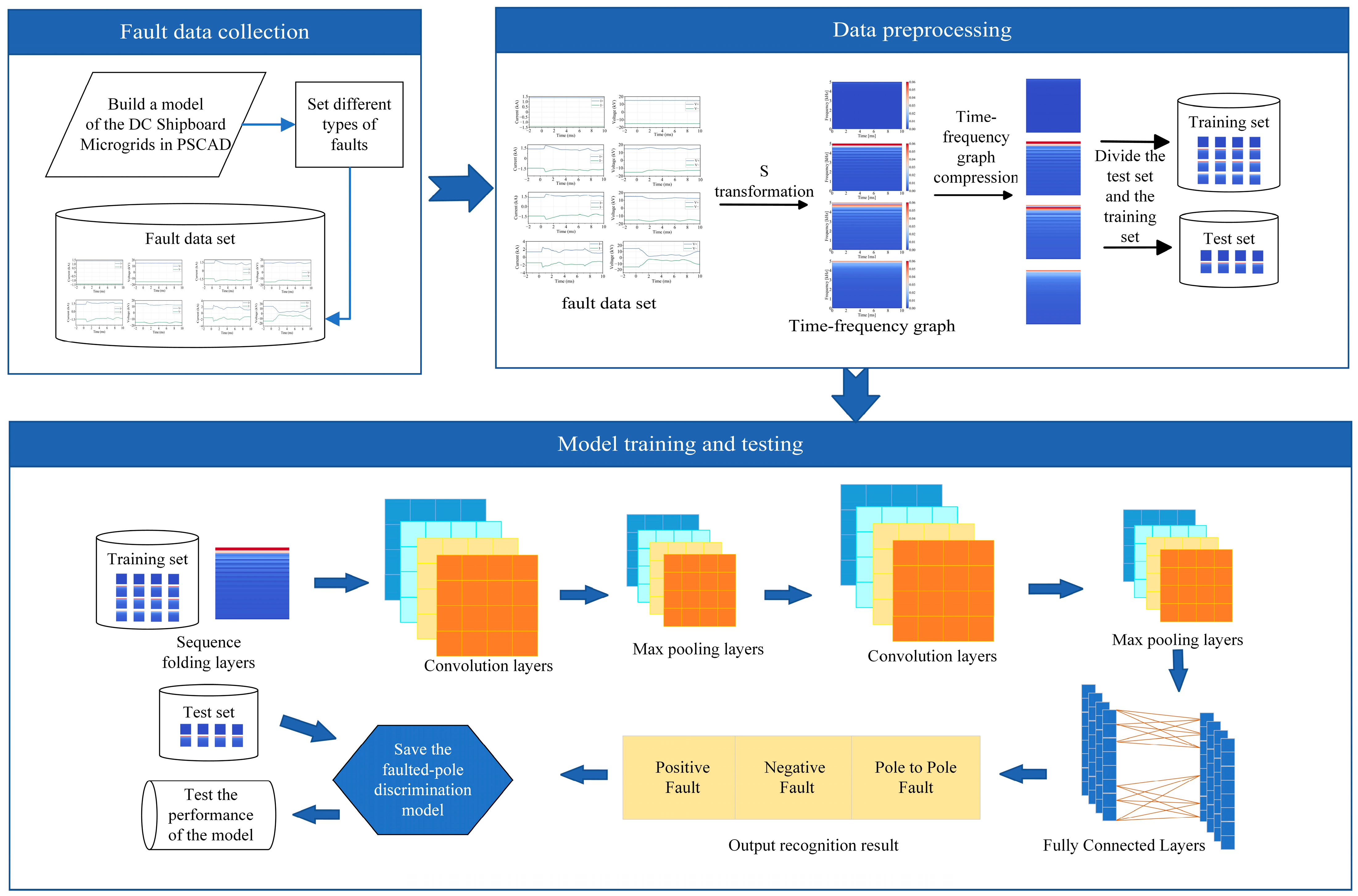
As shown in Figure 3, the proposed faulted-pole discrimination process for shipboard DC microgrid line faults consists of three main stages:

Stage 1: Fault data collection. A detailed shipboard DC microgrid is modeled in PSCAD v4.5. By simulating various operating conditions and fault types, single-ended voltage and current waveforms are collected at the generator terminal during fault transients. These waveforms are used as feature data for training and testing.

Stage 2: Data preprocessing. The collected signals are converted into time–frequency spectrograms using S-Transformation. The spectrograms are resized to fit the CNN input format, and the dataset is split into training and testing subsets.

Stage 3: Model training and testing. A CNN is trained on the processed training data to extract features and classify fault types. The testing set is then used to evaluate the model’s performance.

Figure 3. The flowchart of the faulted-pole discrimination model.

Figure 3. The flowchart of the faulted-pole discrimination model.

4.1. Data Preprocessing

Feature data is obtained by collecting the positive and negative voltage and current data from the generation and rectification end under different operating states, fault locations, and fault types. The obtained feature-data signals are transformed into time–frequency data using S-Transformation, resulting in a two-dimensional time–frequency matrix, where the rows represent the frequency features after time–frequency transformation, and the columns represent the time-feature information.

CNN models require fixed input dimensions. Small images may lose key fault features, while large images increase memory consumption and training time. Additionally, raw signals often contain redundant features. Therefore, selecting appropriate matrix dimensions is crucial.

To ensure timely diagnosis, the first 10 ms of fault data is used, sampled at 10 kHz. Each sample includes four signals: positive and negative voltage and current. Thus, the raw data dimension is 4 × 100. After S-Transformation, FFT-based spectral components reduce the frequency dimension to 50, resulting in a 4 × 50 × 100 spectrogram. For efficiency, the spectrograms are downsampled to 4 × 50 × 50. The compressed time–frequency spectrogram is shown in Figure 4.

4.2. Model Training and Testing

The CNN model training involves three steps: forward propagation, loss calculation, and backward propagation.

4.2.1. Forward Propagation

In the forward propagation stage, the input signal image is passed through the convolutional layer, pooling layer, and fully connected layer in the network, ultimately producing the output. The convolutional layer extracts features through convolution operations using convolutional filters, and an activation function is applied after each convolutional layer to introduce non-linearity. The pooling layer is used to reduce the spatial dimensions of the feature map. The fully connected layer calculates the output through weighted sums and biases, and generates a probability distribution through the softmax activation function. The network computation formula is shown in Equation (9).

$$Q=F_n(\cdots (F_3(F_2(F_1(X{W}_1))W_2)W_3)\cdots W_n)$$

(9)

where $Q$ is the output of the output layer; $F_n$ represents the non-linear transformation performed by each layer; $W_n$ represents the weights of each layer.

4.2.2. Loss Calculation

The loss function measures the difference between the model’s predicted results and the true labels. In classification tasks, a commonly used loss function is the cross-entropy loss function.

$$Loss=-{\displaystyle \sum _{c=1}^c{y}_c·}\log (d_c)$$

(10)

where $c$ is the total number of classes, $y_c$ is the true label of class $c$, and $d_c$ is the probability predicted by the model that the sample belongs to class $c$.

4.2.3. Backward Propagation

In the backpropagation stage, the gradient of each parameter is calculated using the chain rule, as shown in the equation, to determine the contribution of each parameter to the final loss. The weights and biases in the network model during forward propagation are continuously updated using the gradient descent method. The formula is as follows:

$$\left(\begin{array}{l}{W}_{t+1}=W_t-\eta {\displaystyle \frac{\mathsf{\partial }E}{W_t}}\\ b_{t+1}=b_t-\eta {\displaystyle \frac{\mathsf{\partial }E}{b_t}}\end{array}\right.$$

(11)

where $W$ is the weight, $b$ is the weight, $\eta$ is the learning rate, and $E$ represents the error function.

4.3. CNN Parameter Settings

Key CNN parameters include convolution and pooling layers, learning rate, and batch size.

4.3.1. Convolutional Layer and Pooling Layer

The model architecture is based on a simplified version of the VGG network. It includes two convolutional layers and two pooling layers. The first convolutional layer uses a 3 × 1 kernel that slides along the time axis, while the second employs a 3 × 3 kernel that captures joint time–frequency features. Pooling is performed using 2 × 1 kernels, downsampling only along the time dimension. Dropout regularization is applied with rates of 0.3 and 0.4 after the first and second pooling layers, respectively, to mitigate overfitting.

4.3.2. Learning Rate

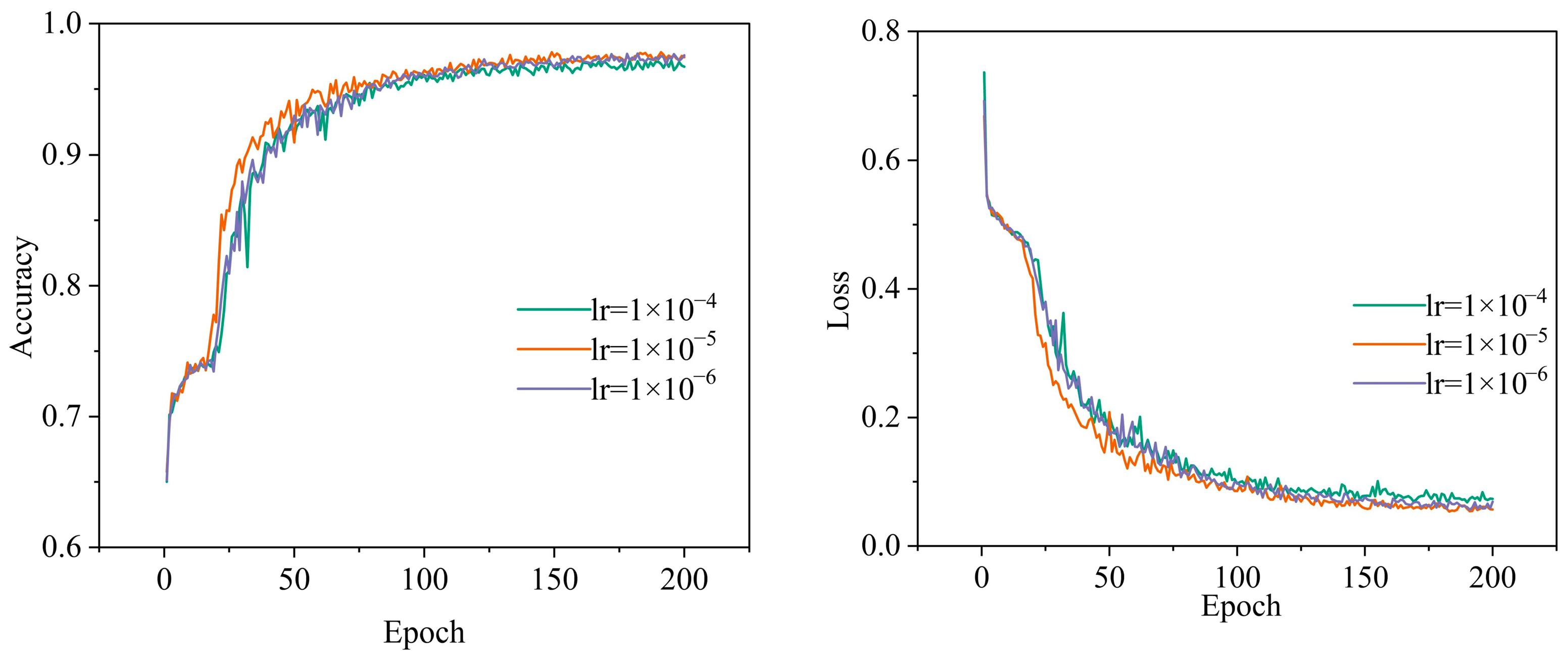
An adaptive learning-rate schedule is employed. The initial rate is set to 0.001. If the validation loss does not improve after three consecutive epochs, the learning rate is reduced by multiplying it by 0.9. To prevent vanishing learning rates, lower bounds of 0.0001, 0.00001, and 0.000001 are tested.

As shown in Figure 5 and

Table 1. Model performance with different learning rates.

Learning-Rate Lower Bound	Training Time/s	Accuracy
0.0001	103.63	0.9821
0.00001	101.81	0.9898
0.000001	121.13	0.9868

, when the learning-rate lower bound is set to 0.00001, the convergence speed, model training time, and test accuracy are all better than the other two cases. Therefore, the learning-rate lower bound chosen in this paper is 0.00001.

The specific formula for calculating accuracy can be expressed as [36]:

$$Accuracy={\displaystyle \frac{TP+TN}{TP+TN+FP+FN}}$$

(12)

In the formula:

TP: The number of samples correctly predicted as positive.

TN: The number of samples correctly predicted as negative.

FP: The number of negative samples incorrectly predicted as positive.

FN: The number of positive samples incorrectly predicted as negative.

4.3.3. Batch Size

Batch size determines how many samples are processed before the model updates its parameters. Three values (16, 32, and 64) are evaluated. Larger batch sizes yield faster training but may reduce generalization. This is because larger batches allow for more efficient parallel computation, speeding up training. However, they may lead to overfitting and reduce the model’s ability to generalize. Smaller batch sizes, while improving accuracy, come with the trade-off of increased computational time due to more frequent updates required during training.

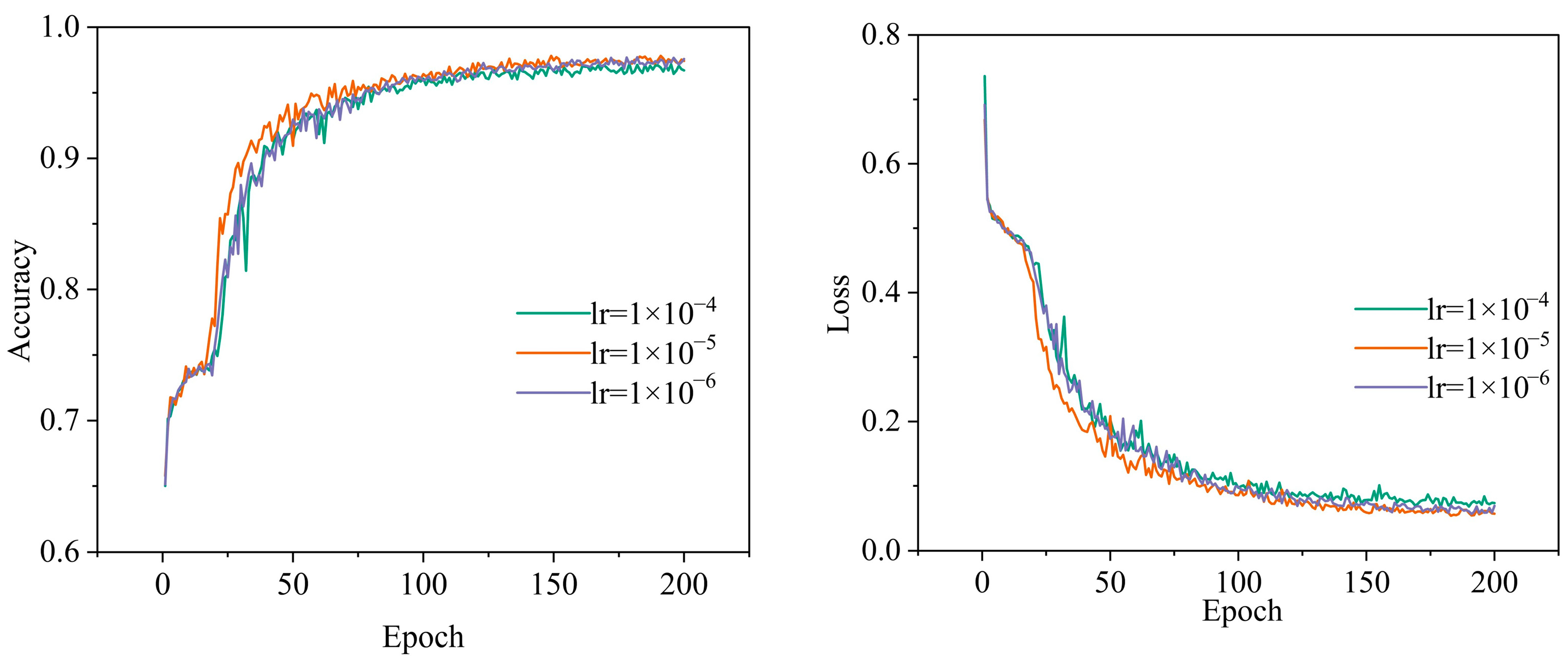
As shown in Figure 6 and

Table 2. Model performance with different batch sizes.

Batch Size	Training Time/s	Accuracy
16	150.31	0.9793
32	103.12	0.9898
64	92.84	0.9821

, when the batch size is 32, although the model training time is 10.28 s longer than when the batch size is 64, the accuracy and loss-function convergence speed are both better than those with a batch size of 64. Therefore, the batch size selected in this paper is 32.

5. Simulation and Verification

The simulation environment is shown in

Table 3. Simulation environment.

Item	Parameter
System version	Windows11 x64
Processor model (CPU)	Intel(R) Core (TM) i5-12600F, Santa Clara, CA, USA
Processing speed	3.7 GHz
Memory (RAM)	16 GB
GPU	RTX3060

, with the network model built using the TensorFlow deep learning framework and Python 3.9 programming language.

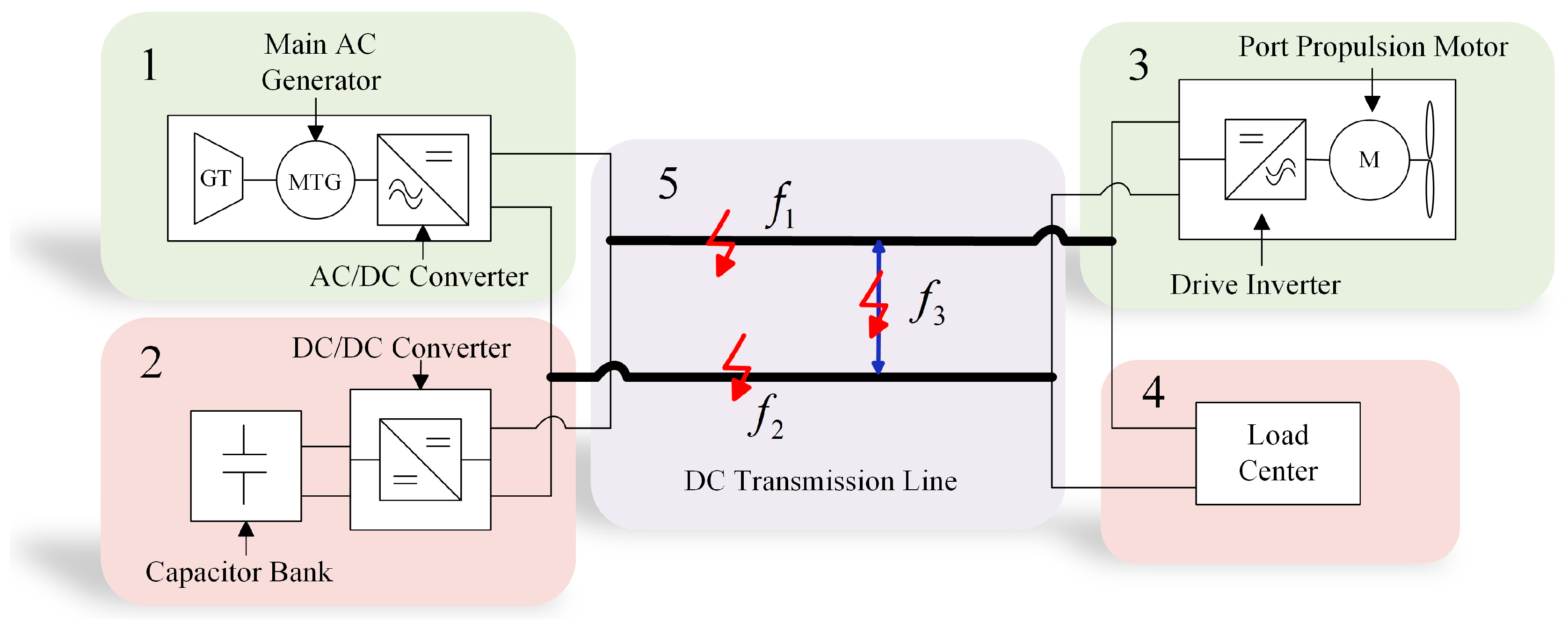
Figure 7 presents the model constructed in PSCAD software, which represents a ±15 kV dual-end, four-terminal system. In this model, element 1 corresponds to the power-generation module of the ship microgrid; 2 denotes the ship microgrid’s energy storage system (ESS); 3 represents the electric propulsion system; 4 indicates the ship’s load center; and 5 refers to the DC transmission line. $f_1$ is a positive-pole fault (PPF), $f_2$ is a negative-pole fault (NPF), and $f_3$ is a pole-to-pole fault (PTPF).

By simulating various operating conditions and fault scenarios, extensive simulations were conducted to generate both training and testing datasets. The specific data are presented in

Table 4. Dataset configurations and parameters.

Parameter	Possible Configuration
Types	PPF, NPF, PTPF
Ship-power load	0, 5%, 10%, 15%, …, 100%
Fault distance	0, 10%, 20%, 30%, …, 100%
Fault resistance (Ω)	0, 5, 10, 20, 40, 50, 80, 100, 150, 200, 250, 300

, covering PPF, NPF, and PTPF cases. The PTPF scenario represents a metallic short-circuit fault, with a fault resistance set to 0 Ω.

5.1. PPF, NPF, and PTPF

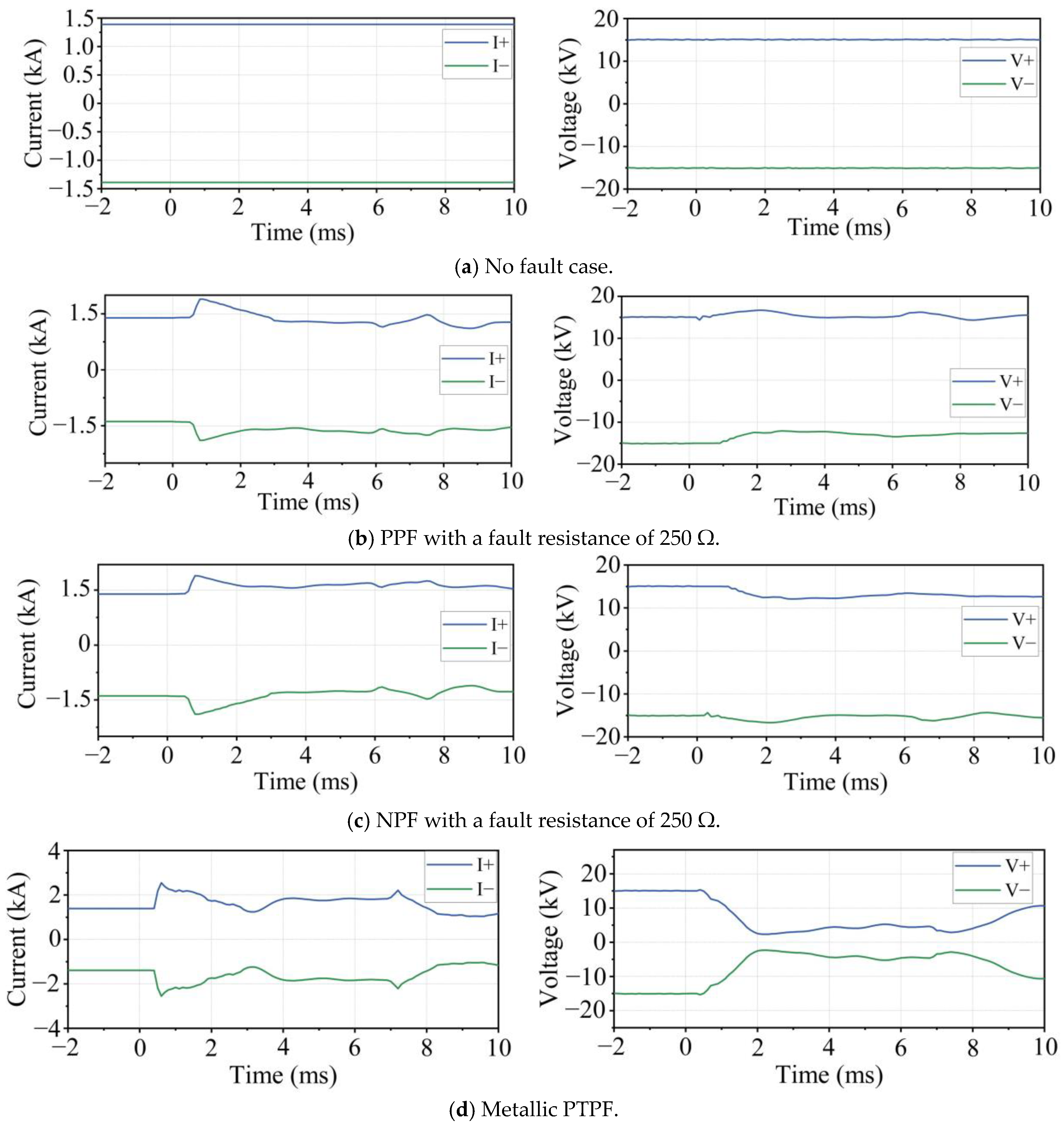
Figure 8 consists of four subplots, all of which present the simulated waveforms of the generator-side terminal under different fault scenarios when the system load is 70% of full capacity. Each subplot contains two parts: the left panel shows the positive or negative line current, while the right panel shows the corresponding voltage. Specifically, Figure 8a shows the normal operating conditions without any fault. Figure 8b,c depict faults occurring at 50% of the line length on the positive and negative lines, respectively, with a fault resistance of 250 Ω. Figure 8d depicts a metallic PTPF.

As illustrated in Figure 8, faults on the line lead to abrupt changes in voltage and current at the generator end. These transient features are extracted and used as input signals for testing the proposed faulted-pole discrimination model. The testing results confirm that the method successfully and accurately identifies all three fault types represented in Figure 8b–d.

It is particularly noteworthy that in Figure 8b,c, the fault currents on the positive and negative lines are highly similar due to the high fault resistance (250 Ω), making it difficult for conventional methods to distinguish between them. However, the proposed method based on S-Transformation and convolutional neural networks accurately discriminates the faulted pole in both cases. This demonstrates the strong robustness and effectiveness of the proposed approach, especially in challenging scenarios where traditional techniques often fail.

5.2. Sensitivity to Fault Distance

When the system load is set to 70% of its full capacity and the fault resistance is fixed at 150 Ω, the performance of the proposed faulted-pole discrimination model under various fault distances is evaluated. The simulation results are summarized in

Table 5. Simulation results for various fault distances.

Fault Distance (%)	Fault Type	Discrimination Result	Fault Type	Discrimination Result	Fault Type	Discrimination Result
0	PPF	PPF	NPF	NPF	PTPF	PTPF
5	PPF	PPF	NPF	NPF	PTPF	PTPF
10	PPF	PPF	NPF	NPF	PTPF	PTPF
20	PPF	PPF	NPF	NPF	PTPF	PTPF
40	PPF	PPF	NPF	NPF	PTPF	PTPF
60	PPF	PPF	NPF	NPF	PTPF	PTPF
90	PPF	PPF	NPF	NPF	PTPF	PTPF
100	PPF	PPF	NPF	NPF	PTPF	PTPF

.

As shown in Table 5, the proposed model consistently achieves accurate faulted-pole identification across different fault locations along the transmission line. This indicates that the model exhibits strong robustness to variations in fault distance and is capable of maintaining high classification performance under diverse spatial-fault conditions.

5.3. Sensitivity to Fault Resistance

To evaluate the method’s robustness to varying fault resistances, simulations are conducted under a fixed fault location at 50% of the line length, with the system load maintained at 70% of its full capacity. The results for different fault-resistance values are presented in

Table 6. Simulation results for various fault resistances.

Fault Resistance (Ω)	Fault Type	Discrimination Result	Fault Type	Discrimination Result
0	PPF	PPF	NPF	NPF
10	PPF	PPF	NPF	NPF
50	PPF	PPF	NPF	NPF
100	PPF	PPF	NPF	NPF
150	PPF	PPF	NPF	NPF
200	PPF	PPF	NPF	NPF
250	PPF	PPF	NPF	NPF
300	PPF	PPF	NPF	NPF

.

As observed in Table 6, the proposed faulted-pole discrimination model maintains high accuracy across a wide range of fault resistances. Even in the case of high-resistance faults, which typically pose challenges to conventional protection schemes, the model continues to deliver reliable identification performance. These results demonstrate that the proposed method is suitable for practical applications where high-resistance faults may occur.

5.4. Comparative Analysis with Existing Classification Models

To further validate the effectiveness of the proposed ship DC microgrid faulted-pole discrimination model, a comparison is made between the model combining S-Transformation and CNN (S-CNN) and traditional fault-classification methods.

• Traditional convolutional neural network (CNN) [37,38];
• CNN combined with Support Vector Machine (CNN-SVM) [39];
• Wavelet Transform combined with CNN (WT-CNN) [40].

The comparative results are shown in

Table 7. Faulted-pole discrimination performance of different models.

Algorithm	Classification Accuracy of Different Defect Types (%)			Total Accuracy (%)	Training Time/s
	PPF	NPF	PTPF
CNN	98.68	95.11	99.53	97.27	168.80
CNN-SVM	60.78	98.02	99.56	71.31	42.57
WT-CNN	93.53	99.12	100.00	96.43	190.47
S-CNN	98.40	99.55	100.00	98.98	103.12

.

As shown in Table 7, the training time for the CNN-SVM model is shorter because CNN is used only for feature extraction and not involved in model training. Additionally, compared to CNN, the training process for SVM is much simpler, resulting in a lower faulted-pole discrimination rate. Overall, the faulted-pole discrimination model combining S-Transformation and CNN outperforms traditional methods in terms of accuracy. Considering both time and accuracy, the faulted-pole discrimination model proposed in this paper has higher accuracy and shorter training and testing times.

6. Conclusions

This paper presents a novel faulted-pole identification method for shipboard DC microgrids based on S-Transformation and CNN. S-Transformation is used to convert voltage and current signals into time–frequency spectrograms, capturing the essential features of fault transients. These spectrograms are compressed and fed into a CNN for classification.

The proposed CNN model improves upon the traditional VGG architecture by optimizing convolutional kernel sizes and selecting effective hyperparameters through a systematic comparison of learning rates and batch sizes. Simulation results show that the proposed method achieves superior fault-classification accuracy and faster training/testing times compared to conventional approaches such as CNN, CNN-SVM, and WT-CNN.

The method proves especially effective under high-resistance and complex fault scenarios, significantly enhancing fault selectivity and robustness. This work provides valuable technical support for real-time faulted-pole detection in next-generation shipboard DC microgrids.

References

1. Yang, Y.; Jin, B.; Liu, Y.; Wei, X.; Wang, K.; Zhang, X. Modeling and Simulation of Medium Voltage DC Power System for All Electric Ships. In Proceedings of the 2024 IEEE 2nd International Conference on Power Science and Technology (ICPST), Dali, China, 9–11 May 2024; IEEE: New York, NY, USA, 2024; pp. 1962–1965. [Google Scholar]
2. Li, Z.; Chen, J.; Li, K.; Xu, Z.; Liu, Y.; Wang, M. Robust Model Predictive Control for Onboard Interleaved Multilevel Boost DC-DC Converter in DC Shipboard Microgrids. IEEE Trans. Transp. Electrif. 2025, 11, 8876–8888. [Google Scholar] [CrossRef]
3. Liu, Y.; Liao, J.; Guo, C.; Tan, Z.; Wang, Y.; Wei, N.; Song, Y. Fault Severity Classification Based Coordination Control Strategy of Fault Current Limiter and Modular Multilevel Converter for Adaptive Fault Current Limiting. J. Mod. Power Syst. Clean Energy 2025, 13, 1432–1443. [Google Scholar]
4. Maydison, H.; Zhang, H.; Han, N.; Oh, D.; Jang, J. Optimized Diesel–Battery Hybrid Electric Propulsion System for Fast Patrol Boats with Global Warming Potential Reduction. J. Mar. Sci. Eng. 2025, 13, 1071. [Google Scholar] [CrossRef]
5. Paipa-Sanabria, E.; González-Montoya, D.; Coronado-Hernández, J.R. Green Technologies for Environmental Air and Water Impact Reduction in Ships: A Systematic Literature Review. J. Mar. Sci. Eng. 2025, 13, 839. [Google Scholar] [CrossRef]
6. Habyarimana, M.; Adebiyi, A.A. A Review of Artificial Intelligence Applications in Predicting Faults in Electrical Machines. Energies 2025, 18, 1616. [Google Scholar] [CrossRef]
7. Wang, T.; Zhang, C.; Hao, Z.; Monti, A.; Ponci, F. Data-driven Fault Detection and Isolation in DC Microgrids Without Prior Fault Data: A Transfer Learning Approach. Appl. Energy 2023, 336, 120708. [Google Scholar] [CrossRef]
8. Yang, Y.; Tu, F.; Huang, S.; Tu, Y.; Liu, T. Research on CNN-LSTM DC Power System Fault Diagnosis and Differential Protection Strategy Based on Reinforcement Learning. Front. Energy Res. 2023, 11, 1258549. [Google Scholar] [CrossRef]
9. Yousaf, M.Z.; Khalid, S.; Tahir, M.F.; Tzes, A.; Raza, A. A novel dc fault protection scheme based on intelligent network for meshed dc grids. Int. J. Electr. Power Energy Syst. 2023, 154, 109423. [Google Scholar] [CrossRef]
10. Shanmugapriya, V.; Vidyasagar, S.; Raju, D.K. Post-fault voltage recovery and voltage instability assessment of DC microgrid with Deep Transfer-learning Convolution Neural Network. Electr. Power Syst. Res. 2025, 239, 111234. [Google Scholar] [CrossRef]
11. Bayati, N.; Balouji, E.; Baghaee, H.R.; Hajizadeh, A.; Soltani, M.; Lin, Z.; Savaghebi, M. Locating high-impedance faults in DC microgrid clusters using support vector machines. Appl. Energy 2022, 308, 118338. [Google Scholar] [CrossRef]
12. Liu, T.; Yan, J.; Liu, Y.; Chung, C.Y. Cascading Failure Screening Based on Gradient Boosting Decision Tree for HVDC Sending-End Systems with High Wind Power Penetration. IEEE Trans. Power Syst. 2025, 99, 1–13. [Google Scholar] [CrossRef]
13. Salehimehr, S.; Miraftabzadeh, S.M.; Brenna, M. A novel machine learning-based approach for fault detection and location in low-voltage DC microgrids. Sustainability 2024, 16, 2821. [Google Scholar] [CrossRef]
14. Chen, Q.; Wu, J.; Li, Q.; Gao, X.; Yu, R.; Guo, J.; Yang, B. Long short-term memory network-based HVDC systems fault diagnosis under knowledge graph. Electronics 2023, 12, 2242. [Google Scholar] [CrossRef]
15. Dash, P.K.; Pattnaik, S.R.; Prasad, E.N.; Bisoi, R. Detection and classification of DC and feeder faults in DC microgrid using new morphological operators with multi-class AdaBoost algorithm. Appl. Energy 2023, 340, 121013. [Google Scholar] [CrossRef]
16. Yin, Z.; Wang, L.; Yang, S.; Gao, Y. A series arc fault diagnosis method in DC distribution systems based on multiscale features and random forests. IEEE Sens. J. 2022, 23, 2605–2617. [Google Scholar] [CrossRef]
17. Deb, A.; Jain, A.K. An effective data-driven machine learning hybrid approach for fault detection and classification in a standalone low-voltage DC microgrid. Electr. Eng. 2024, 106, 6199–6212. [Google Scholar] [CrossRef]
18. Veerapandiyan, S.; Sugavanam, V. On-line fault identification, location, and seamless service restoration using transfer learning-based convolution neural network for low-voltage DC microgrid. Electr. Power Compon. Syst. 2023, 51, 785–808. [Google Scholar] [CrossRef]
19. Li, J.; Song, G.; Yan, J.; Li, Y.; Xu, Z. Data-driven Fault Detection and Classification for MTDC Systems by Integrating HCTSA and Softmax Regression. IEEE Trans. Power Deliv. 2021, 37, 893–904. [Google Scholar] [CrossRef]
20. Yang, Y.; Tai, N.; Fan, C.; Yang, L.; Chen, S. Resonance Frequency-based Protection Scheme for Ultra-High-Voltage Direct-Current Transmission Lines. IET Gener. Transm. Distrib. 2018, 12, 318–327. [Google Scholar] [CrossRef]
21. Xu, Y.; Liu, J.; Fu, Y. Fault-Line Selection and Fault-Type Recognition in DC Systems Based on Graph Theory. Prot. Control Mod. Power Syst. 2018, 3, 27. [Google Scholar] [CrossRef]
22. Rahmani, R.; Sadeghi, S.H.H.; Askarian-Abyaneh, H.; Emadi, M.J. An entropy-based scheme for protection of DC microgrids. Electr. Power Syst. Res. 2024, 228, 110010. [Google Scholar] [CrossRef]
23. Salehi, M.; Taher, S.A.; Sadeghkhani, I.; Shahidehpour, M. A poverty severity index-based protection strategy for ring-bus low-voltage DC microgrids. IEEE Trans. Smart Grid 2019, 10, 6860–6869. [Google Scholar] [CrossRef]
24. Tiwari, R.S.; Sharma, J.P.; Gupta, O.H.; Ahmed Abdullah Sufyan, M. Extension of pole differential current based relaying for bipolar LCC HVDC lines. Sci. Rep. 2025, 15, 16142. [Google Scholar] [CrossRef]
25. Shamsoddini, M.; Vahidi, B.; Razani, R.; Mohamed, Y.A.R.I. A novel protection scheme for low voltage DC microgrid using inductance estimation. Int. J. Electr. Power Energy Syst. 2020, 120, 105992. [Google Scholar] [CrossRef]
26. Ma, J.; Xiao, Z.; Cheng, P. A pilot protection scheme for flexible HVDC transmission lines based on modulus power. Int. J. Electr. Power Energy Syst. 2022, 137, 107849. [Google Scholar] [CrossRef]
27. Chu, X.; Lv, H. Coupling characteristic analysis and a fault pole detection scheme for single-circuit and double-circuit HVDC transmission lines. Electr. Power Syst. Res. 2020, 181, 106179. [Google Scholar] [CrossRef]
28. An, N.; Shu, H.; Yang, B.; Cao, P.; Song, J.; Guo, Y. Voltage Correlation Based Single Pole-to-Ground Fault Detection of MMC-HVDC Transmission Line. IEEE Access 2020, 9, 118124–118133. [Google Scholar] [CrossRef]
29. Qin, H.; Peng, F.; Pan, Z.; Zhong, Y.; Liu, T.; Cao, R. A Single-Ended Protection Scheme for Flexible HVDC Transmission Lines Based on the Fréchet Distance of the Rate of Change of Fault Voltage Traveling Waves. IEEE Access 2025, 13, 128716–128728. [Google Scholar] [CrossRef]
30. Farshad, M. Detection and classification of internal faults in bipolar HVDC transmission lines based on K-means data description method. Int. J. Electr. Power Energy Syst. 2019, 104, 615–625. [Google Scholar] [CrossRef]
31. Lazzari, R.; Piegari, L.; Grillo, S.; Carminati, M.; Ragaini, E.; Bossi, C.; Tironi, E. Selectivity and Security of DC Microgrid Under Line-to-Ground Fault. Electr. Power Syst. Res. 2018, 165, 238–249. [Google Scholar] [CrossRef]
32. Datta, S.; Chattopadhyaya, A.; Chattopadhayay, S.; Das, A. S-transform based kurtosis analysis for detection of LG and LL faults in 14 Bus microgrid system. IETE J. Res. 2022, 68, 3766–3777. [Google Scholar] [CrossRef]
33. Mishra, S.; Gupta, S.; Yadav, A.; Abdelaziz, A.Y. Traveling wave-based fault localization in FACTS-compensated transmission line via signal decomposition techniques. Energies 2023, 16, 1871. [Google Scholar] [CrossRef]
34. Song, G.; Cheng, J.; Grattan, K.T.V. Recognition of microseismic and blasting signals in mines based on convolutional neural network and stockwell transform. IEEE Access 2020, 8, 45523–45530. [Google Scholar] [CrossRef]
35. Alzubaidi, L.; Zhang, J.; Humaidi, A.J.; Al-Dujaili, A.; Duan, Y.; Al-Shamma, O.; Santamaría, J.; Fadhel, M.A.; Al-Amidie, M.; Farhan, L. Review of deep learning: Concepts, CNN architectures, challenges, applications, future directions. J. Big Data 2021, 8, 53. [Google Scholar] [CrossRef] [PubMed]
36. Bacevicius, M.; Paulauskaite-Taraseviciene, A. Machine learning algorithms for raw and unbalanced intrusion detection data in a multi-class classification problem. Appl. Sci. 2023, 13, 7328. [Google Scholar] [CrossRef]
37. Liu, Y.; Zhu, Y.; Wu, K. CNN-based Fault Phase Identification Method of Double Circuit Transmission Lines. Electr. Power Compon. Syst. 2020, 48, 833–843. [Google Scholar] [CrossRef]
38. Lan, S.; Chen, M.J.; Chen, D.Y. A Novel HVDC Double-Terminal Non-Synchronous Fault Location Method Based on Convolutional Neural Network. IEEE Trans. Power Deliv. 2019, 34, 848–857. [Google Scholar] [CrossRef]
39. Gnanamalar, A.J.; Bhavani, R.; Arulini, A.S.; Veerraju, M.S. CNN–SVM Based Fault Detection, Classification, and Location of Multi-Terminal VSC–HVDC System. J. Electr. Eng. Technol. 2023, 18, 3335–3347. [Google Scholar] [CrossRef]
40. Paul, D.; Mohanty, S.K. Fault Classification in Transmission Lines Using Wavelet and CNN. In Proceedings of the 2019 IEEE 5th International Conference for Convergence in Technology (I2CT), Pune, India, 29–31 March 2019; IEEE: New York, NY, USA, 2019; pp. 1–6. [Google Scholar]
Figure 1. The time–frequency spectrogram of positive-pole current via S-Transformation.
Jmse 13 01510 g001
Figure 2. The structure of a typical CNN.
Jmse 13 01510 g002
Figure 4. Compressed time–frequency spectrogram.
Jmse 13 01510 g004
Figure 5. Training curves under different learning rates.
Jmse 13 01510 g005
Figure 6. Training curves under different batch sizes.
Jmse 13 01510 g006
Figure 7. Simulated ship DC microgrid model.
Jmse 13 01510 g007
Figure 8. Simulation results of different faults.
Jmse 13 01510 g008