Abstract
Turbidity currents pose significant threats to offshore seabed infrastructures, including subsea hydrocarbon production facilities and submarine communication cables. These powerful underwater flows can damage pipelines, potentially causing hydrocarbon spills that endanger local communities, the environment, and negatively impact energy production infrastructures. Therefore, a comprehensive understanding of the spatio-temporal development and destructive force of turbidity currents is essential. While numerical computation of 3D flow, sediment transport, and substrate exchange is possible, field-scale simulations are computationally intensive. In this study, we develop a simplified morphodynamic approach to model the flow properties of channelized turbidity currents and the associated trends of sediment accretion and erosion. This model is applied to the Baco–Malaylay submarine system to investigate the dynamics of a significant turbidity current event that impacted a submarine pipeline offshore the Philippines. The modeling results align with available seabed assessments and observed erosion trends of the protective rock berm. Our simplified modeling approach shows good agreement with simulations from a fully 3D numerical model, demonstrating its effectiveness in providing valuable insights while reducing computational demands.
1. Introduction
Sediments typically travel downhill from a continental source to an oceanic sink. From the coastal region, which extends to the edge of the continental shelf, sediment is transported to the deep marine environment primarily by turbidity currents. These gravity-driven underflows, generated by the excess density associated with the dispersed phase, travel downslope, eroding and incising the continental slope [1,2,3,4] and finally depositing sediment onto the continental rise and abyssal plain, forming some of the world’s largest sediment accumulations [5,6,7]. Turbidity currents, which may travel at speeds in excess of ~20 m/s [8,9], pose a tangible threat to offshore seafloor facilities (e.g., communication cables and pipelines), potentially causing network connection issues and/or loss of hydrocarbon containment, with negative impacts on energy security, communication networks, and safety risks to local communities. Even relatively dilute and low-velocity turbidity currents may generate scours around seafloor structures, which can be technically challenging to remedy in deep water settings. Turbidity current events persist over extended periods, as evidenced by measurements within the Congo submarine channel, where flow durations ranged from several weeks in the proximal part of the system [10] to several weeks in the distal sections [11].
Numerical modeling of turbidity currents can address significant scientific and operational challenges. Computational fluid dynamics (CFD) 3D simulations are powerful tools for investigating the dynamics of single turbidity current events over natural topographies [12,13,14,15]. However, the computational cost of these simulations is strongly related to the number of computational cells, which depends on the size of the area of interest and the desired model resolution. In practice, the resolution required for 3D computational grids can become a major obstacle, as highly resolved numerical models may require hours or days per simulation, even with powerful computers. As a consequence, the majority of 3D numerical simulations of turbidity currents are performed at laboratory scale [16,17]. Additionally, various sources of uncertainty must be considered when modeling turbidity currents. These currents can be triggered by different mechanisms, such as breaching [18], hyperpycnal currents driven by rivers in flood [9,19], typhoon-induced nearshore circulation [14], and mega-rip currents [15]. Consequently, the frequency of these mechanisms, initial conditions, location, and upstream boundary conditions in numerical simulations are considerably uncertain, necessitating the testing of multiple plausible scenarios. Furthermore, numerical models, regardless of their complexity, rely on empirical closure relations for determining sediment entrainment from the bed into suspension (e.g., [20]), which are based on laboratory data and have intrinsic uncertainties and limitations when applied at field scale. Additionally, sediment availability along the flow path and at the channel head plays a crucial role in the dynamics of turbidity currents and is often not entirely known. Testing these uncertain parameters and scenarios increases the computational power and time required for 3D simulations.
Given the factors discussed above, particularly for domains larger than tens of kilometers, it is evident that simplified turbidity current modeling approaches (e.g., [21]) may represent a powerful tool to gain insight on turbidity currents activity in a specific area. These models can provide indeed a practical and efficient means to understand the spatial development of turbidity currents without the high computational costs associated with detailed 3D simulations. On the other hand, two-dimensional vertical models (e.g., [22]) or layer averaged models that do not account for the spatial variation in the canyon width (e.g., [23,24,25]) cannot describe the pattern of erosion and deposition associated with the full complexity of canyon morphology. In this contribution, we describe a channel centerline-based turbidity current morphodynamic modeling approach that is used to reconstruct the bulk-flow properties of a significant turbidity current that impacted a submarine pipeline offshore the Philippines in December 2016. To complement conventional industry risk assessments, the results of this modeling effort are part of a broader multidisciplinary study investigating the root cause and dynamics of turbidity current activity in the area [14].
The structure of the paper is as follows: Section 2 outlines the mathematical formulation of the developed turbidity currents morphodynamic model. Section 3 introduces the study area (i.e., the Baco–Malaylay submarine system), highlighting the recent turbidity current activity, and presenting a detailed analysis of the down-channel morphological data used to inform the modeling. Section 4 presents the results of the model application, while Section 5 discusses the findings and concludes the study.
2. The Morphodynamic Model
Morphodynamics is the process by which the Earth’s surface movable bed morphology and hydrodynamics interact and evolve over time. This field addresses the problems arising from the evolution of bed morphology due to variations in sediment erosion and deposition patterns induced by the overlying flow-field, which itself changes dynamically in response to the evolving morphology. To accurately describe the morphodynamics of submarine channels, it is essential to couple the turbidity current flow-field (including fluid phase continuity, momentum, and suspended sediment mass conservation) with an evolution equation for the movable bed interface.
2.1. Governing Equations
Our formulation builds upon the gradually varied flow-field model introduced in [26], which is based on the foundational work presented in [27]. We consider the steady motion of a dilute, multi-size sediment class turbid underflow in a submarine channel with a seabed slope and active width . In a one-dimensional modeling framework, the conservation equations for the hydrodynamics of steady turbidity currents over a sloping channel are as follows:
where x is the streamwise down-channel coordinate locally tangent to the seabed, g is the acceleration due to gravity, and R is the sediment submerged specific gravity (e.g., 1.65 for quartz). U and h are bulk turbidity current velocity and thickness, respectively, whereas is the depth-averaged volumetric suspended sediment concentration, with the specific contribution of each sediment size class. Moreover, , , and are the sediment entrainment rate coefficient, the volume fraction bed composition, the near-bed concentration, and the settling velocity of the i-th sediment size class, respectively. Other quantities include the shear velocity , the water entrainment coefficient , and the bulk settling velocity of the mean (geometric) value of the suspended sediment particles, which is used to estimate the detrainment of water from the turbid underflow in the water conservation Equation (1). Finally, and represent the lateral flux of water and sediment away from the channel above the levee crest (Figure 1).
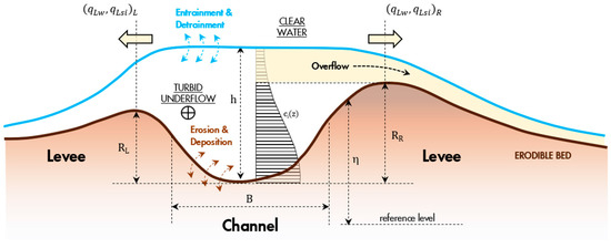
Figure 1.
Channel cross-section illustrating water entrainment and detrainment across the turbid interface, along with sediment entrainment and deposition processes from and to the erodible bed. The sketch also depicts a typical concentration profile and the portion of the sediment column that overspills above the levee crest. In the numerical model, the cross-section is assumed to be rectangular, with the dominant flow direction perpendicular to the cross-section.
Turbidity currents deposits are then modeled by coupling the conservation Equations (1)–(3) with the Exner sediment balance equation describing the evolution of the movable bed interface. For each sediment size class composing the mixture, we can write
where is the rate of variation in seabed elevation associated with each sediment particle diameter class, with the local value of the seabed elevation relative to some horizontal datum, whereas and are the i-th size class sediment porosity and bedload transport volume rate, respectively.
Within the above presented modeling framework, the flow is assumed to be steady, nonuniform on hydrodynamic timescales, whereas, on morphologic timescales, it is allowed to evolve due to the net sediment erosion and deposition of the underlying temporally varying seabed.
2.2. Closure Relationships
To solve the full morphodynamic problem (1–4), a set of closure relationships is required. Entrainment of clear water into the current is modeled following [28]. Sediment entrainment from the bed can be estimated using relations derived from open-channel flow settings, verified for turbidity currents (e.g., [29,30,31]), or the Partheniades formulation [32]. The near-bed concentration ratio of the (i)-th sediment class is evaluated using Garcia’s closure relationship [33]. Shear velocity is assumed proportional to the bulk-flow-averaged velocity through a constant flow conductance factor , incorporating all flow frictional effects: . Particle settling velocity is computed using relationships from the literature (e.g., Seminara and Tubino [34] fitting Parker’s data [35]). Bedload transport intensity is estimated by using empirical or semi-empirical relationships (e.g., [36,37]). Lateral flow overspill above channel levees is computed by extending classical overbank flow relations to turbidity flows [26]. Sediment overspill is estimated following [38] and [39], who showed that vertical concentration profiles in turbidity currents are analogous to those in fluvial environments, following the classical Rouse profile [26].
3. Application
3.1. Study Area
In the northeastern part of Mindoro Island, the Malaylay and Baco Rivers flow into the Verde Island Passage (VIP), a strait between Luzon and Mindoro Islands (Figure 2). The shallow shelf area at the river mouths is very narrow, averaging only a few hundred meters. This limited space for sediment accumulation creates a nearly direct link between the river mouths and the submarine canyons in deeper waters, facilitating the travel of submarine mass gravity flows to the basin [14].
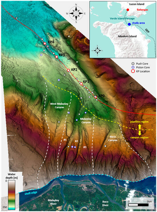
Figure 2.
Bathymetry map (2017 survey) and satellite image of the study area. The white dashed lines indicate the influence areas of the three main canyons on the Baco–Malaylay slope: West-Malaylay, Malaylay, and Baco. The yellow dashed line marks the boundary between the canyon and pipeline regions discussed in the text. The black dashed line represents the pipeline as built in 2001, while the red line shows its current position. Note that displacements occurred after the first turbidity current event impacted the GEP in 2006. Gray dots indicate the locations of sediment samples collected during the 2017 campaign, with push cores outlined in black and piston cores outlined in blue. White dots with red outlines show the relative locations of GEP KPs. The dashed cyan line represents the approximate 10 m isobath; no detailed bathymetric surveys are available for the inner-shelf area.
Additionally, a submarine gas export pipeline (GEP) runs through the eastern part of Mindoro Island, crossing the VIP to reach onshore processing facilities in Batangas Bay (Figure 2).
The northern seafloor of Mindoro Island, just offshore from the mouth of the Baco–Malaylay river system, can be divided into two main regions: the canyon region and the pipeline region (Figure 2). The canyon region encompasses the Baco–Malaylay continental slope, which is carved by numerous channels starting approximately 250 m from the coastline (possibly closer). These channels merge down the slope to form three larger canyons: the West-Malaylay, Malaylay, and Baco canyon systems (Figure 2). According to [14], the seafloor of these canyons shows alternating bands of erosion and deposition. These characteristic seafloor features, with wavelengths between 20 and 120 m (average 55 m) and heights of 2 to 4 m, are interpreted as upslope migrating bedforms primarily formed by turbidity current activity.
In contrast, the pipeline region consists of a wider, relatively flat-floored valley formed by the merging of the Malaylay and Baco canyon systems. This valley features a notable constriction near Kilometer Point 4 (KP4) (Figure 2). Similarly to the canyon region, the pipeline region is characterized by alternating areas of sediment deposition and erosional scours. These seabed features, with wavelengths of about 100–200 m and heights of 1.5–2 m, have a semicircular, downslope-elongated shape with downstream concavity (Figure 3, top and middle). This shape, along with the analysis of their internal structure from Sub-Bottom Profile (SBP) data, suggests that the bedforms in the pipeline region also migrate counter to the main flow direction (i.e., upslope), with sediment deposited on the upstream (stoss) side and eroded from the downstream (lee) side (Figure 3, bottom). Further evidence of the erosion and deposition pattern in the pipeline region is seen in the alternating emergent and buried sections of the rock berm installed in 2009 to protect the GEP (Figure 3, middle).
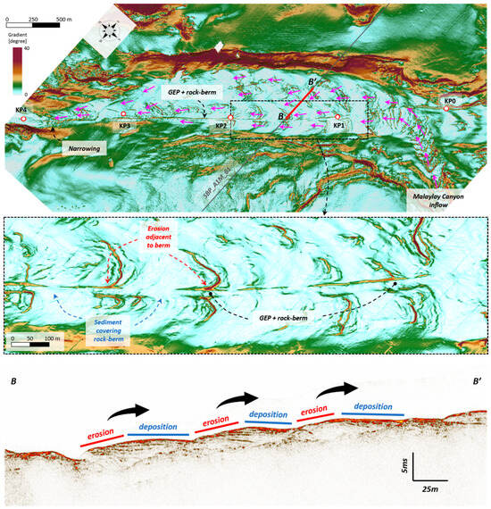
Figure 3.
Top: Detail of the 2017 bathymetric data (sea floor dip magnitude) focused on the pipeline region. Magenta arrows indicate turbidity current flow directions deduced from geomorphological indicators such as scours and lineations. The flow enters from the Malaylay canyon and is predominantly oriented from right to left. The steeper lateral edges of the rock berm protecting the GEP (approximately 2 m above the surrounding seafloor) are clearly resolved in the bathymetric slope map. White dots with red outlines indicate the relative locations of GEP KPs, while the gray line represents the Sub-Bottom Profiler (SBP) data shown in the bottom panel. Middle: Detail of the pipeline region showing the distribution of erosional scours and depositional areas close to the rock berm. The berm topography actively shapes the bedform pattern adjacent to the GEP. Bottom: Segment of SBP data revealing the internal stratigraphy of the bedform pattern. Red bars mark the stoss side where erosion has occurred, and blue bars indicate zones of dominant deposition on the lee side of the bedforms. Black arrows highlight the direction of bedform migration, which is opposite to the main flow (magenta arrows in the top image).
3.2. Turbidity Currents Activity
Since its installation in 2001, the GEP has experienced two significant turbidity current events in the Malaylay canyon system (2006 and 2016) that have threatened its integrity. These events were triggered by sediment resuspension in the shallow shelf area in front of the Malaylay and Baco river mouths, transported into the canyon heads by typhoon-induced waves and currents [14]. The first event, associated with Typhoon Durian in December 2006, caused the displacement of the GEP at two locations (KP0-1 and KP3-4, see Figure 2). The second event, which is the focus of this paper, was triggered by nearshore circulation induced by Typhoon Nock-ten in December 2016 and damaged the rock berm installed in 2009 to protect the KP0-4 segment of the GEP.
Streamwise profiles digitized along the main channels were used to extract the temporal evolution of the seafloor from multiple bathymetric surveys. These data reveal that the turbidity current induced by Typhoon Nock-ten displayed simultaneous flow activity in multiple channels just offshore from the mouth of the Baco–Malaylay river system. As shown in Figure 4, during the 2011–2017 period, the digitized profiles of all major channels in the Malaylay canyon system exhibit significant bathymetric changes, indicating activity between the two surveys. Specifically, the bedforms in channel #1 migrated more than one wavelength, while those in channels #2 and #3 showed upstream migration of up to half a wavelength. The thalweg of channel #1 was completely reshaped between the 2011 and 2017 seabed surveys, suggesting it was the most active of the three coalescent channels forming the Malaylay canyon during this period. The sediment transport process responsible for the bedform migration could have occurred at any time during the 2011–2017 interval, but it is reasonable to assume that most changes resulted from the major 2016 turbidity current triggered by Typhoon Nock-ten. In contrast, no significant bathymetric changes were detected during the 2007–2008 and 2008–2011 periods, indicating that the Malaylay canyon system was essentially inactive during those times.
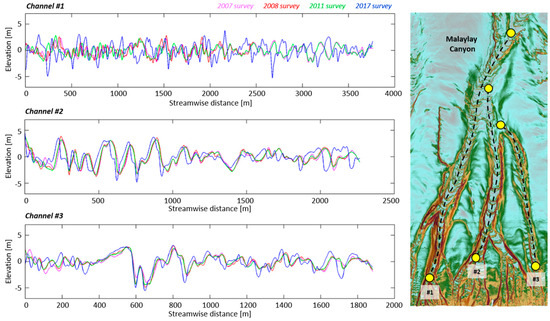
Figure 4.
Left: Downslope development of bedform elevations in the main channels (#1−2−3) of the Malaylay canyon, highlighting temporal changes in the seabed measured through repeated bathymetric surveys (2007, 2008, 2011, 2017). Right: Digitized streamwise profiles of channels #1−2−3 used to extract bathymetric changes over time. Magnitude slope color scale is the same as in Figure 3.
The West-Malaylay and Baco canyon systems exhibited minimal activity during the 2007–2008 and 2008–2011 periods. Clear signs of upstream migrating bedforms were only observed during the 2011–2017 period, indicating activity likely associated with Typhoon Nock-ten. However, the amplitude of these bedforms diminishes downslope, suggesting that flows through these channels dissipated before reaching the pipeline region [14]. This evidence points to the Malaylay canyon as the source of the 2016 turbidity current, with channel #1 serving as the main pathway for the current that impacted the pipeline.
3.3. Morphological Data Analysis
As discussed in Section 3.2., only flows passing through the Malaylay canyon system, located in the central part of the slope, are believed to have impacted the GEP during the Nock-ten-induced turbidity current event. To estimate its destructive force, the turbidity currents morphodynamic model described in Section 2 has been specifically applied to channel #1, identified as the most active of the three coalescent channels forming the Malaylay canyon.
Within the current modeling framework, various topographic and morphological attributes need to be estimated to compute the down-channel distribution of the turbidity current bulk-flow properties. These attributes include (i) the bed elevation profile along a prescribed channel centerline path, (ii) the spatial (down-channel) distribution of the channel width, and (iii) the downstream variation in channel bank heights along the channel path. These morphological attributes have been extracted from the available digital bathymetry, starting from the shelf-break, following the path of channel #1 down the slope, and continuing along the main canyon of the bend-valley region (Figure 5).
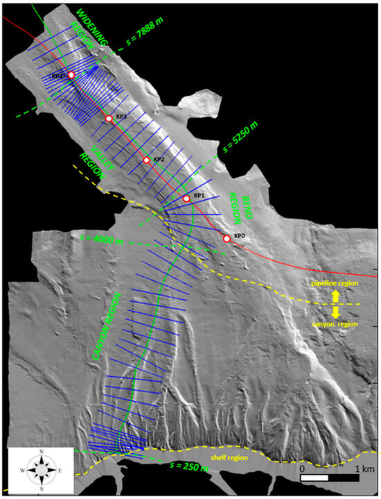
Figure 5.
Hillshade representation of the 2009 (i.e., post rock berm installation) bathymetric data. Superimposed are centerline path (green line), current position of the GEP (red line), analyzed cross-sections, and major reference KPs. Main regions along flow path and associated streamwise coordinate (s) are also represented: i.e., the canyon, bend, valley, and widening region.
The centerline bed elevation profile has been computed by interpolating the topographic elevation of the bathymetry data at centerline coordinates. Several cross-sections perpendicular to the channel axis (Figure 5) have been manually analyzed to determine the local width of the channel and the heights of the levee crests to the left and right of the centerline.
Figure 6 illustrates the down-channel distributions of bed elevation, channel width, levee heights, and channel gradient used in the numerical simulation to model the spatial development of the turbidity current. Along its approximately 9 km pathway, starting at the shelf-break (~250 m offshore from the river mouth), the Malaylay system exhibits a concave-up bathymetric profile, ranging from ~10 m to about 380 m in water depth. Downdip from the shelf-break, four distinct reaches can be identified: the canyon region (as previously defined), and within the pipeline region, the bend region, the valley region, and the widening region (Figure 5).
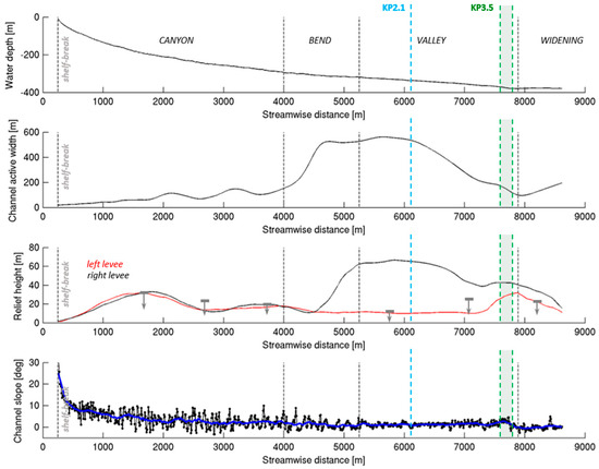
Figure 6.
Upper panel: longitudinal elevation of the seabed along the analyzed centerline (Figure 5). Second panel: extracted spatial distribution of the channel active width. Third panel: down−channel variation in channel levee heights with respect to local channel thalweg. Gray markers indicate estimated flow thickness range as interpreted from 2017 SBP data. Bottom panel: down−channel slope (black dotted line represents raw data, while blue line shows the smoothed trend obtained using a moving average). All panels: light blue dashed line indicates location at which canyon floor starts to narrow; green shaded area between dashed green lines indicates the region where the GEP rock berm was most seriously impacted by the 2016 event (associated pipeline KP are also indicated).
The canyon region is approximately 3.75 km long, with an average slope of ~4.4° (0.077) and a maximum slope of about 25° (0.436) just downdip from the shelf-break. In this reach, the channel width increases from about 20 m to roughly 150 m, while the channel bank height remains relatively symmetric between the right and left margins. In the upper part of the canyon region, where the channel relief increases faster than the channel width, cross-sections generally exhibit an incised shape with no depositional levees (Figure 7). The absence of bedforms along inter-canyon areas (Figure 7, right) supports the interpretation that turbidity currents become channelized (i.e., confined) almost immediately upon entering the slope [14]. Conversely, in the lower part of the canyon region, channel relief decreases to a more constant value of about 15–20 m (Figure 6), suggesting turbidity currents spill over the channel banks (Figure 7). The transition from strong reflectivity at the channel floor and lack of layering to layered deposits on the channel banks is interpreted as the shift from dominant erosion flows at the channel base to overbank deposition higher up on the channel margins and overbank (Figure 7, middle panel).
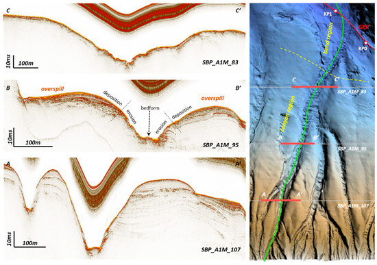
Figure 7.
Three east–west 2017 SBP lines in the canyon region along the centerline (green line) show different patterns. In section AA’, the channel walls suggest minimal flow overspill, indicating a thinner flow than the channel relief. Section BB’ shows erosion in the lower channel walls and deposition in the upper walls, suggesting recent flows reached or slightly exceeded channel limits. Section CC’ indicates coarser material with low penetration, and possibly some suspended sediment layering on the left side of the channel walls.
The transition from the canyon region to the valley region is marked by an abrupt change in direction from northeast to northwest (Figure 5). In this relatively short (~1.2 km) curved flow path, the channel gradient remains roughly constant at ~1.2° (0.021). The channel width progressively increases to about 500 m, and the levee height becomes highly asymmetric, with lower relief on the inner margin of the bend (Figure 6 and Figure 8). This area was of particular concern during the construction of the rock berm in 2009. The 2006 Typhoon Durian-induced event severely impacted the integrity of the GEP at this location, causing a displacement of the unprotected pipeline by 110 m off its axis between KP0-1 (Figure 2 and Figure 8, right).
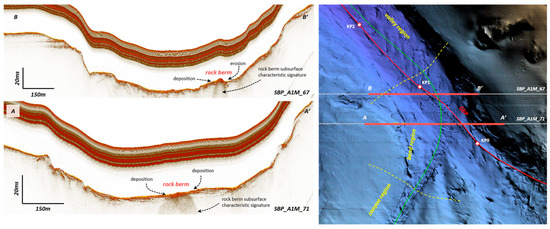
Figure 8.
Details of different east–west 2017 SBP lines in the bend region. Channel levees heights become asymmetric with the inner bank lower than the outer. No signature of significant overbank deposition can be observed. Note that the 2009 installed protective rock berm is preserved after the 2016 turbidity current event. Erosional scours and depositional areas close to the rock berm are mainly associated with the migration of preexisting bedforms. A green line represents the analyzed centerline.
The valley region spans approximately 2.6 km with a mean slope angle of ~1.3° (0.023). The absence of significant in-channel net depositional patterns (Figure 8) suggests that flows in this region are either slightly erosional or in equilibrium with the seabed morphology, with sedimentation dominated by migrating bedforms (Figure 3). The correlation between channel slope and densimetric Froude number [40] indicates that the flow is primarily supercritical, reinforcing the non-depositional character of the flow. In the proximal part of the valley region, the channel width remains roughly constant at about 550 m. Around KP2.1, the canyon floor begins to narrow, reaching a minimum width of about 100 m just upstream of KP4 (Figure 6). Channel levee heights are highly asymmetric (Figure 6 and Figure 9): the right flank is steep and about 60 m high, likely preventing significant spillover from turbidity currents. Conversely, the left channel wall dips gently, with a fairly constant levee height of about 10 m, allowing the upper part of the turbidity current to potentially overspill and deposit fine-grained particles in the overbank area. However, significant overbank deposition is only evident downstream of KP3 (Figure 9). As the channel approaches its narrowest section, the left flank steepens, creating a higher levee crest that progressively enhances flow confinement (Figure 6 and Figure 9). This promotes localized in-channel erosion, emphasized by the simultaneous rapid narrowing of the channel and a localized increase in gradient (~2.7°, 0.047) (Figure 6, green area). At this location (~KP3.5–3.7), the rock berm was completely eroded by the 2016 turbidity current event, leaving the pipeline unprotected (upper left SBP section of Figure 9). This occurred precisely where a 42 m pipeline displacement was found after the 2006 event (Figure 2). Downstream of KP3.7, the channel gradient suddenly drops, becoming nearly horizontal and leading to enhanced sediment deposition.
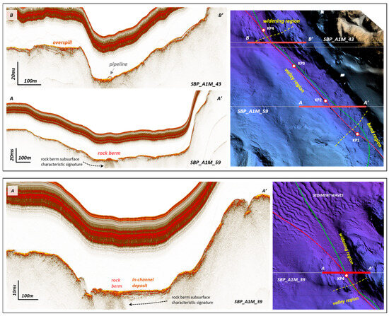
Figure 9.
Details of different east–west 2017 SBP lines in the valley (top panel) and widening (bottom panel) regions. In the valley region, channel levees heights are very asymmetric, and clear signature of overspill deposition are only evident in the left overbank area close to the narrowest section (i.e., downstream KP3). Note that in section BB’ the GEP is unprotected with the rock berm completely eroded by the Nock-ten event. In the widening region, in-channel sediment deposition is promoted. Note that the rock berm has been buried by sediment showing the depositional nature of the 2016 turbidity current event in this area. Green line represents the analyzed centerline.
Turbidity currents entering the widening region (Figure 5 and Figure 9) are primarily depositional, as indicated by the relatively thick deposits blanketing the seafloor immediately downslope of the narrowest section (Figure 9 bottom and Figure 10). In this region, the channel width expands, and the mean channel gradient is reduced to ~0.02° (~3 × 10⁻⁴). Additionally, levee heights decrease, and turbid underflows become progressively unconfined. Downstream of KP4, the deposit is sharply truncated by an erosional cut, promoted by a localized increase in the seabed slope (~4.9°, 0.082). The GEP’s integrity was not affected in this region by either the 2006 or 2016 events. The final run-out length of turbidity currents cannot be precisely inferred from seabed data analysis due to the presence of seafloor sediment waves in the more distal part of the widening region (Figure 9 and Figure 10). These sediment waves are likely the result of reworking of turbidite deposits by bottom currents with strong tidal components flowing from the N-NE across the area.
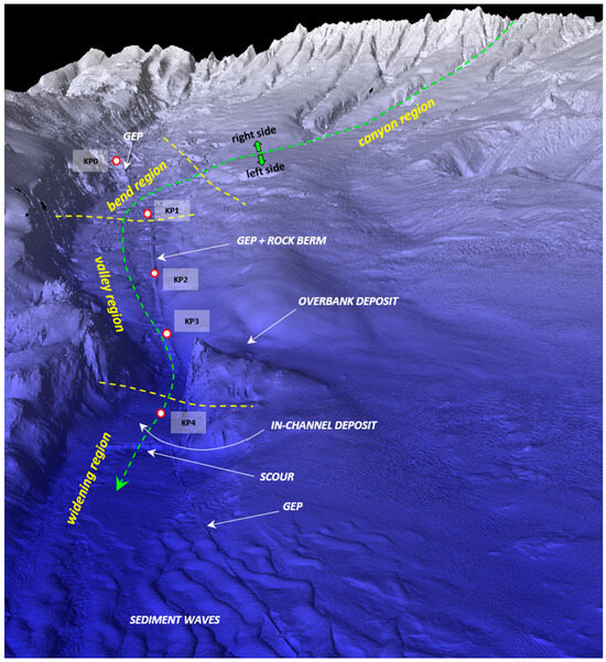
Figure 10.
Three-dimensional view of the seabed (2017 survey). Note the presence of sediment waves disturbing the seafloor in the distal part of the widening region. Dotted green line represents conceptualized turbidity current path.
4. Results
When modeling turbidity currents the choice of appropriate upstream boundary conditions, namely, flow velocity, flow depth, suspended sediment concentration, and partitioning between different sediment classes (when polydisperse solutions are employed) is a nontrivial task which usually requires further modeling. Following the innovative methodology described in [14], Nock-ten inflow boundary conditions at the head of the canyon (i.e., at the shelf-break) were derived by coupling available typhoon hindcast data with a sediment resuspension and transport model [41]. The values at peak conditions during the Nock-ten typhoon have been used as upstream boundary conditions, namely, flow velocity = 0.62 m/s, flow thickness = 2.8 m, and total suspended sediment concentration = 0.00169 (97% mud and 3% sand). Inflow sediment mixture has been modeled by employing two sediment classes with diameter 20 μm and 150 μm, representative for mud and sand, respectively. These values for the sediment grain size were consistent with observations from a set of push cores (35) and piston cores (8) collected during the 2017 campaign (see Figure 2 for core locations).
The sediment entrainment relationship plays a crucial role in determining the spatial development of the turbidity current along the entire canyon system. Regardless of the complexity employed to describe the flow-field, numerical models rely on laboratory-based empirical closure relations for determining sediment entrainment from the bed into suspension. These relations exhibit considerable variability and possess some inherent limitations when applied at field scale. Building on the work presented in [26], where the hydrodynamic model was successfully validated against both laboratory-scale and field-scale turbidity current measurements, we adopted the Partheniades sediment entrainment predictor to maintain consistency and ensure reliability within the established modeling framework:
where is the erosion flux for the i-th sediment size, is the sediment density, τ is the bed shear stress, and is critical shear stress for entrainment. Observed Nock-ten-related mean erosional trends have been used to constrain the entrainment into suspension of the coarse fraction (Table 1). Moreover, in agreement with observations from seabed cores, in-channel sediment composition has been assumed uniformly distributed and equal to 1% for the mud component and 99% for the sand.

Table 1.
Summary of model inputs.
As detailed in Section 2, the friction factor is defined in terms of flow conductance , which incorporates all flow-related frictional effects, such as skin friction of the bed, form drag caused by bedforms, and additional drag at the interface between turbid water and clear water. The friction factor is typically variable and, even in the absence of other drag forces beyond friction, flow conductance depends on factors like water depth. Nevertheless, for simplicity, this analysis assumes a constant flow conductance. Although the hypothesis of constant friction can be easily modified, it is deemed a reasonable assumption when modeling first-order (i.e., bulk) turbidity current properties, particularly under conditions where the spatial development of flow thickness changes gradually along the channel, as observed in this case study. A specific flow conductance value was employed in the numerical simulation. This choice is consistent with empirical data for sand-bed-dominated channels [42,43] and with a first-order estimate of composite flow roughness height comparable to observed bedforms, yielding modeled flow thicknesses that align well with both SBP observations and sediment core data. Table 1 summarizes the necessary modeling inputs used to estimate the first-order bulk-flow properties associated with the Nock-ten turbidity current event.
Figure 11 illustrates the modeled spatial development of bulk-flow properties during the Nock-ten event. The flow accelerates from the shelf-break through the canyon region, reaching a peak velocity of approximately 6 m/s before decelerating in the bend region to a steady velocity of around 4 m/s in the upper-middle valley region. As the flow approaches the narrowest section in the lower valley region, velocity increases again, with a maximum of approximately 5.7 m/s observed between KP3.5–3.7 (indicated by the green area in Figure 11). The modeled flow thickness generally remains below the levee crests, with spillover from turbidity current predicted only in the lower valley region where the upper part of the modeled flow surpasses the elevation of the left bank. These results align with SBP observations and sediment core data. Further validation of the modeled flow properties is provided by seabed observations and rock berm erosion processes linked to the Nock-ten event, verified directly from the available data.
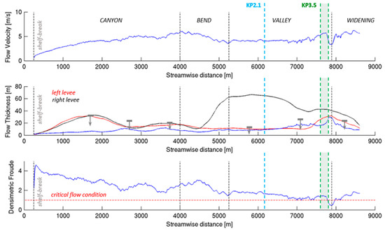
Figure 11.
Spatial development of bulk-flow properties for the reference simulation. Top panel: flow velocity. Middle panel: flow thickness; gray markers indicate estimated flow thickness range as interpreted from SBP data. Bottom panel: flow densimetric Froude number. All panels: green area indicates the region where the GEP rock berm was most seriously impacted by the 2016 event; light blue dashed line indicates the location at which canyon floor starts to narrow.
4.1. Comparison with Seabed Assessments
Trends of sediment accretion and erosion associated with the turbidity current induced by Typhoon Nock-ten were evaluated through a comparative analysis of available bathymetric surveys conducted before and after the 2016 event. For the valley region, a difference map was generated by subtracting the 2009 bathymetry (post rock berm installation) from the most recent survey data obtained in 2017. The resulting difference map is illustrated in Figure 12 (top). Although areas of both erosion (red) and deposition (blue) are observed, seabed activity related to the 2016 event exhibits a slightly erosional trend (0.60 m ± 0.25 m). The uncertainty in the observed mean deposit is comparable to the precision of water-depth measurements across the surveys. Figure 12 (bottom panel) presents a comparison between modeled and observed seabed changes associated with the 2016 event in the valley region. Modeling of the Nock-ten turbidity current flow assumed a duration of approximately 45 min, consistent with [14]. The model accurately captures the overall trend, predicting a mean erosional pattern of about 0.59 m. Notably, the model forecasts significant erosion between KP3.5–3.7, corresponding to the precise location where the rock berm was eroded during Typhoon Nock-ten.
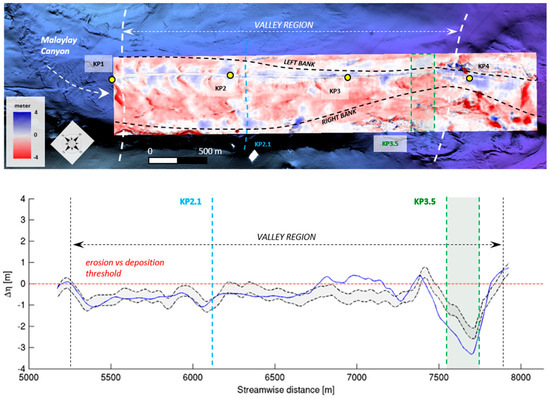
Figure 12.
Top: Observed seabed erosion (red color) and deposition (blue color) pattern associated with the Nock-ten turbidity current event along the valley region and the proximal reach of the widening. Black dashed lines indicate the channel banks defining the active channel width used in the numerical simulation. Bottom: Predicted (blue line) versus observed (gray envelope) width−averaged erosion/deposit associated with the 2016 event; the gray envelope accounts for the uncertainty in the observed trend including absolute errors in water-depth measurements from the different surveys. In both panels, the green area indicates the region where the GEP rock berm was most seriously impacted by the 2016 event, whereas a light blue dashed line indicates location at which canyon floor starts to narrow.
Results from the numerical simulation have further supported the interpretation of anti-dune characteristics of the bedforms present in both the canyon and valley regions of the Malaylay Canyon. Based on their dimensions, migration patterns, and estimated flow thickness, these bedforms may be classified as either anti-dunes or cyclic steps [14]. Anti-dunes are bedforms that develop in supercritical flow regimes, whereas cyclic steps are bedforms associated with transcritical flows on steep slopes. The modeling provides clear evidence that, under sustained flow conditions, a supercritical regime prevails from the head of the canyon to the lower part of the valley region (refer to Figure 11, bottom panel). The modeled flow attains near-critical conditions just upstream of KP3.5 and becomes distinctly sub-critical close to the narrowest section. It is important to note that this modeling effort focused on the most intense and large stage of the turbidity current flow associated with the Nock-ten typhoon at peak conditions. Transitions from sub-critical to supercritical flow along individual bedforms cannot be ruled out under less intense conditions associated with weaker but more frequent turbidity currents or during the waning stages of the largest turbidity currents. Smaller-scale turbidity currents that do not extend to the valley may flow over the short-wavelength bedforms of the canyon region in a cyclic steps mode. Further studies using fully 3D CFD simulations are required to ascertain whether such transcritical flows may occur along these bedforms.
4.2. Comparison with Observed ROCK Berm Erosion
The pipeline survey conducted in early 2017 highlighted the impact of the Nock-ten turbidity current event on the protective rock berm. In the bend region and the more proximal part of the valley between KP1.6 and KP2.1, the turbidity current had minimal impact on the rock berm. Between KP2.1 and KP3.5, some localized erosion processes occurred due to the narrowing of the canyon, yet the berm remained largely intact with no evidence of berm material being transported by the turbidity current. The most significant effects of the 2016 turbidity current were observed between KP3.5 and KP3.7, where the rock berm was eroded away, leaving the GEP exposed (see Figure 9 top panel, SBP section BB’). Further downstream, the berm appears to be intact and buried by sediment (see Figure 9 bottom panel, SBP section AA’).
The numerically simulated shear velocity (Figure 13) predicts the transport of rock berm material predominantly in the more distal part of the valley region near the narrowest section (i.e., between KP3.5 and KP3.7), which aligns with observations of berm erosion. The critical shear condition for the transport of rock berm sediment, specifically eclogite boulders with a mean diameter of 0.13 m and a density of 3200 kg/m3, was estimated using the classical Brownlie relation [44]. A comparison with the spatial development of the shear velocity as predicted by employing a fully 3D numerical model is also illustrated in Figure 13. The computational fluid dynamics 3D numerical simulation was performed using the TCsolver code [12,13,45,46,47]] under the same Nock-ten inlet peak conditions [14]. Despite the simplifications inherent in the centerline-based morphodynamic model, the agreement between the shear velocity behavior predicted by the two different models throughout the entire valley region is noteworthy.
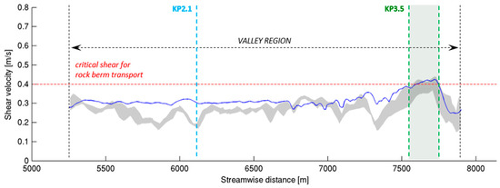
Figure 13.
The predicted Nock-ten shear velocity in the valley region is shown. The blue line represents the centerline-based reference simulation, while the gray envelope curves depict the TCsolver results extracted from an area near the centerline path. The red dashed line indicates the critical shear velocity associated with the incipient transport condition of the protective-berm boulders. The green area in the graph denotes the region where the GEP rock berm was completely removed during the Nock-ten event.
5. Discussion and Conclusions
A centerline-based morphodynamic model for the investigation of channelized turbidity currents flowing over natural topographies has been presented. Using a gradually varied modeling approach, the hydrodynamic problem is solved considering the flow as a steady state polydisperse suspension [26]. Sediment accretion and erosion patterns are modeled by coupling the flow-field solution with an appropriate version of the Exner equation of sediment conservation. This framework assumes the hydrodynamic time-scale (i.e., the rate at which the flow adjusts to a new topography) is much smaller than the morphodynamic timescale (i.e., the rate at which bottom topography adjusts to the new flow-field), which holds true under sustained, suspended-load-dominated flow conditions [11,48], the focus of this study. In addition to the steady state hypothesis of the flow-field, the model here presented is based on a number of approximations. The flow is assumed to be one-dimensional; hence the effects of secondary flows on channel bends and their effects on the main along channel flow are neglected. Moreover, the cross-section is represented as rectangular; hence variations in flow and sediment bed compositions along the transverse direction are not accounted for. Finally, the shallow water approximation is employed, and the suspended sediment concentration is assumed sufficiently small to allow for the Boussinesq approximation.
As part of a comprehensive multidisciplinary study (see [14]), which investigates the root cause, return period, and dynamics of turbidity current activity in the Malaylay canyon system, the model has been effectively used to reconstruct flow properties and associated patterns of sediment erosion and deposition of a significant typhoon-induced turbidity current that impacted the Malampaya GEP in December 2016. The primary sources of uncertainty were the appropriate estimates of inflow conditions, erosion fluxes, and bed roughness. Inflow boundary conditions were derived by integrating available typhoon hindcast data with a sediment resuspension and transport model [14] and directly incorporating them into the turbidity current model. Conversely, sediment entrainment from the sand bed and flow conductance were constrained using observed mean erosional trends and interpreted flow thickness, respectively. Modeled bulk-flow properties and erosion and deposition trends are consistent with the available data. Specifically, a relative peak in flow velocity and sediment bed erosion is predicted between KP3.5–3.7. At this location, the rock berm protecting the GEP was found to be washed away following typhoon Nock-ten’s passage in December 2016. Additionally, in agreement with observations, the modeled flow transport capacity accurately predicts the movement of rock berm material only where the rock berm sustained damage. Furthermore, numerical simulation results align with the interpreted anti-dune nature of the bedforms on the seafloor of the Malaylay system. Lastly, the reliability of the modeled flow properties is further assured by the good correlation between the spatial development of shear velocity as predicted by the current modeling approach and a fully 3D numerical model.
Despite the simplifications, the adopted modeling approach has proven then to be a powerful tool for gaining insight on the destructive force of turbidity currents and their induced erosion and sedimentation processes. With limited computational effort, extensive simulations (e.g., Monte Carlo experiments) can be performed to investigate the impact of physically plausible assumption on turbidity currents dynamics. Integrating simulation results with conventional structural reliability analyses enables the formulation of early recommendations for safe installation zones of subsea facilities. This approach can identify critical areas that may warrant further, more detailed, and computationally intensive studies, thus ensuring efficient and effective allocation of resources. By proactively identifying these critical areas, the environmental risks associated with hydrocarbon spills resulting from pipeline failures can be mitigated. Such spills can lead to severe ecological damage, affecting marine life, coastal habitats, and local communities. The loss of hydrocarbons not only poses a threat to the environment but also disrupts energy production and can have long-lasting consequences on the sustainability of offshore operations. Therefore, integrating these analyses is crucial for safeguarding both the marine ecosystem and the reliability of subsea infrastructures.
Author Contributions
Conceptualization, A.F. and M.B.P.; methodology, A.F. and M.B.P.; formal analysis, A.F.; investigation, all authors; data curation, A.F., M.B.P., O.E.S., and C.P.; writing—original draft preparation, A.F.; writing—review and editing, all authors. All authors have read and agreed to the published version of the manuscript.
Funding
This research received no external funding.
Data Availability Statement
In this study, no new data sources were used with respect to the ones included in [14] and its supplementary information files. The complete geophysical and geotechnical datasets were acquired by Shell and are proprietary to Shell. Due to the sensitivity of the matter, full access to these datasets is restricted and can be granted upon reasonable request only by Shell Global Solutions International B.V.
Acknowledgments
The authors thank Shell Philippines Exploration B.V. for partially funding this study. Initial geological and sedimentological support from Douglas G. Masson and Philip Weaver is also acknowledged.
Conflicts of Interest
The Authors Alessandro Frascati, Octavio Sequeiros were employed by the company Shell Global Solutions International B.V. The Author Alessandro Cantelli was employed by the company Shell International Exploration and Production Inc. The remaining authors declare that the research was conducted in the absence of any commercial or financial relationships that could be construed as a potential conflict of interest.
Abbreviations
The following abbreviations are used in this manuscript:
| CFD | Computational Fluid Dynamics |
| VIP | Verde Island Passage |
| GEP | Gas Export Pipeline |
| KP | Kilometer Point |
| SBP | Sub-Bottom Profile |
References
- Pirmez, C.; Beaubouef, R.; Friedmann, S.; Mohrig, D. Equilibrium profile and base level in submarine channels: Examples from late Pleistocene systems and implications for the architecture of deepwater reservoirs. In Global Deep-Water Reservoirs: Gulf Coast Section SEPM Foundation 20th Annual, Proceedings of the Perkins Research Conference, Houston, TX, USA, 3–6 December; Bob, F., Ed.; SEPM: Palm Harbor, FL, USA, 2000; pp. 782–805. [Google Scholar]
- Beaubouef, R.T.; Friedmann, S.J. High Resolution Seismic/Sequence Stratigraphic Framework for the Evolution of Pleistocene Intra Slope Basins, Western Gulf of Mexico: Depositional Models and Reservoir Analogs; Deep-Water Reservoirs of the World, Paul Weimer SEPM Society for Sedimentary Geology: Claremore, OK, USA, 2000. [Google Scholar] [CrossRef]
- Paull, C.K.; Ussler, W., III; Caress, D.W.; Lundstein, E.; Barry, J.; Covault, J.A.; Maier, K.L.; Xu, J.; Augenstein, S. Origins of large crescent-shaped bedforms within the axial channel of Monterey Canyon. Geosphere 2010, 6, 755–774. [Google Scholar] [CrossRef]
- Meiburg, E.; Kneller, B. Turbidity currents and their deposits. Annu. Rev. Fluid Mech. 2010, 42, 135–156. [Google Scholar] [CrossRef]
- Bouma, A.H.; Normark, W.R.; Barnes, N.E. Submarine Fans and Related Turbidite Systems; Springer: New York, NY, USA, 1985. [Google Scholar]
- Deptuck, M.E.; Piper, D.J.W.; Savoye, B.; Gervais, A. Dimensions and architecture of late Pleistocene submarine lobes off the northern margin of East Corsica. Sedimentology 2008, 55, 869–898. [Google Scholar] [CrossRef]
- Talling, P.J.; Masson, D.G.; Sumner, E.J.; Malgesini, G. Subaqueous sediment density flows: Depositional processes and deposit types. Sedimentology 2012, 59, 1937–2003. [Google Scholar] [CrossRef]
- Piper, D.J.W.; Cochonat, P.; Morrison, M.L. The sequence of events around the epicentre of the 1929 Grand Banks earthquake: Initiation of debris flows and turbidity current inferred from sidescan sonar. Sedimentology 1999, 46, 79–97. [Google Scholar] [CrossRef]
- Liu, J.T.; Wang, Y.-H.; Yang, R.J.; Hsu, R.T.; Kao, S.-J.; Lin, H.-L.; Kuo, F.H. Cyclone-induced hyperpycnal turbidity currents in a submarine canyon. J. Hydraul. Res. 2012, 117, C04033. [Google Scholar] [CrossRef]
- Azpiroz-Zabala, M.; Cartigny, M.J.B.; Talling, P.J.; Parsons, D.R.; Sumner, E.J.; Clare, M.A.; Simmons, S.M.; Cooper, C.; Pope, E.L. Newly recognized turbidity current structure can explain prolonged flushing of submarine canyons. Sci. Adv. 2017, 3, e1700200. [Google Scholar] [CrossRef] [PubMed]
- Baker, M.L.; Talling, P.J.; Burnett, R.; Pope, E.L.; Ruffell, S.C.; Urlaub, M.; Clare, M.A.; Jenkins, J.; Dietze, M.; Neasham, J.; et al. Seabed seismographs reveal duration and structure of longest runout sediment flows on Earth. Geophys. Res. Lett. 2024, 51, e2024GL111078. [Google Scholar] [CrossRef]
- Abd El-Gawad, S.; Cantelli, A.; Pirmez, C.; Minisini, D.; Sylvester, Z.; Imran, J. Three-dimensional numerical simulation of turbidity currents in a submarine channel on the seafloor of the Niger Delta slope. J. Geophys. Res. 2012, 117, C05026. [Google Scholar] [CrossRef]
- Abd El-Gawad, S.; Cantelli, A.; Pirmez, C.; Minisini, D.; Sylvester, Z.; Imran, J. 3-D numerical simulation of turbidity currents in submarine canyons off the Niger Delta. Mar. Geol. 2012, 326, 55–66. [Google Scholar] [CrossRef]
- Sequeiros, O.E.; Pittaluga, M.B.; Frascati, A.; Pirmez, C.; Masson, D.G.; Weaver, P.; Crosby, A.R.; Lazzaro, G.; Botter, G.; Rimmer, J.G. How typhoons trigger turbidity currents in submarine canyons. Sci. Rep. 2019, 9, 9220. [Google Scholar] [CrossRef]
- Porcile, G.; Pittaluga, M.B.; Frascati, A.; Sequeiros, O.E. Typhoon-induced megarips as triggers of turbidity currents offshore tropical river deltas. Commun. Earth Environ. 2020, 1, 2. [Google Scholar] [CrossRef]
- Georgoulas, A.N.; Angelidis, P.B.; Panagiotidis, T.G.; Kotsovinos, N.E. 3D numerical modelling of turbidity currents. Environ. Fluid Mech. 2010, 10, 603–635. [Google Scholar] [CrossRef]
- Meiburg, E.; Radhakrishnan, S.; Nasr-Azadani, M. Modeling Gravity and Turbidity Currents: Computational Approaches and Challenges. Appl. Mech. Rev. 2015, 67, 040802. [Google Scholar] [CrossRef]
- Van den Berg, J.H.; Van Gelder, A.; Mastbergen, D.R. The importance of breaching as a mechanism of subaqueous slope failure in fine sand. Sedimentology 2002, 49, 81–95. [Google Scholar] [CrossRef]
- Mulder, T.; Syvitski, J.P.; Migeon, S.; Faugères, J.-C.; Savoye, B. Marine hyperpycnal flows: Initiation, behavior and related deposits. A review. Mar. Pet. Geol. 2003, 20, 861–882. [Google Scholar] [CrossRef]
- Garcia, M.; Parker, G. Experiments on the entrainment of sediment into suspension by a dense bottom current. J. Geophys. Res. 1993, 98, 4793–4807. [Google Scholar] [CrossRef]
- Traer, M.; Fildani, A.; McHargue, T.; Hilley, G. Simulating depth-averaged, one-dimensional turbidity current dynamics using natural topographies. J. Geophys. Res. 2015, 120, 1485–1500. [Google Scholar] [CrossRef]
- Felix, M. Flow structure of turbidity currents. Sedimentology 2002, 49, 397–419. [Google Scholar] [CrossRef]
- Ma, H.; Parker, G.; Cartigny, M.; Viparelli, E.; Balachandar, S.; Fu, X.; Luchi, R. Two-layer formulation for long-runout turbidity currents: Theory and bypass flow case. J. Fluid Mech. 2025, 1009, A19. [Google Scholar] [CrossRef]
- Traer, M.M.; Fildani, A.; Fringer, O.; McHargue, T.; Hilley, G.E. Turbidity current dynamics: 1. Model formulation and identification of flow equilibrium conditions resulting from flow stripping and overspill. J. Geophys. Res. Earth Surf. 2018, 123, 501–519. [Google Scholar] [CrossRef]
- Traer, M.M.; Fildani, A.; Fringer, O.; McHargue, T.; Hilley, G.E. Turbidity current dynamics: 2. Simulating flow evolution toward equilibrium in idealized channels. J. Geophys. Res. Earth Surf. 2018, 123, 520–534. [Google Scholar] [CrossRef]
- Bolla Pittaluga, M.; Frascati, A.; Falivene, O. A gradually varied approach to model turbidity currents in submarine channels. J. Geophys. Res. 2018, 123, 80–96. [Google Scholar] [CrossRef]
- Parker, G.; Fukushima, Y.; Pantin, H.M. Self-accelerating turbidity currents. J. Fluid Mech. 1986, 171, 145–181. [Google Scholar] [CrossRef]
- Parker, G.; Garcia, M.; Fukushima, Y.; Yu, W. Experiments on turbidity currents over an erodible bed. J. Hydraul. Res. 1987, 25, 123–147. [Google Scholar] [CrossRef]
- García, M.; Parker, G. Entrainment of bed sediment into suspension. J. Hydraul. Eng. 1991, 117, 414–435. [Google Scholar] [CrossRef]
- Böttner, C.; Stevenson, C.J.; Englert, R.; Schönke, M.; Pandolpho, B.T.; Geersen, J.; Feldens, P.; Krastel, S. Extreme erosion and bulking in a giant submarine gravity flow. Sci. Adv. 2024, 10, eadp2584. [Google Scholar] [CrossRef]
- Smith, J.D.; McLean, S.R. Spatially averaged flow over a wavy surface. J. Geophys. Res. 1977, 82, 1735–1746. [Google Scholar] [CrossRef]
- Partheniades, E. Erosion and deposition of cohesive soils. J. Hydraul. Div. 1965, 91, 105–139. [Google Scholar] [CrossRef]
- Garcia, M. Depositional turbidity currents laden with poorly sorted sediment. J. Hydraul. Eng. 1994, 120, 1240–1263. [Google Scholar] [CrossRef]
- Seminara, G.; Tubino, M. Sand bars in tidal channels. Part 1. Free bars. J. Fluid Mech. 2001, 440, 49–74. [Google Scholar] [CrossRef]
- Parker, G. Self–formed rivers with stable banks and mobile bed: Part I, The sand–silt river. J. Fluid Mech. 1978, 89, 109–126. [Google Scholar] [CrossRef]
- Meyer-Peter, E.; Mueller, R. Formulas for bed-load transport. In Proceedings of the 2nd Meeting of the International Association for Hydraulic Structure Research, Stockholm, Sweden, 7–9 June 1948; pp. 39–64. [Google Scholar]
- van Rijn, L.C. Sediment transport, part I: Bed load transport. J. Hydraul. Eng. 1984, 110, 1431–1456. [Google Scholar] [CrossRef]
- Bolla Pittaluga, M.; Imran, J. A simple model for vertical profiles of velocity and suspended sediment concentration in straight and curved submarine channels. J. Geophys. Res. 2014, 119, 483–503. [Google Scholar] [CrossRef]
- de Leeuw, J.; Eggenhuisen, J.T.; Cartigny, M.J.B. Linking submarine channel–levee facies and architecture to flow structure of turbidity currents: Insights from flume tank experiments. Sedimentology 2018, 65, 931–951. [Google Scholar] [CrossRef]
- Sequeiros, O.E. Estimating turbidity current conditions from channel morphology: A Froude number approach. J. Geophys. Res. 2012, 117, C04003. [Google Scholar] [CrossRef]
- van Rijn, L.C.; Walstra, D.J.R.; van Ormondt, M. Description of TRANSPOR2004 and Implementation in Delft3D-Online; Final Report (Prepared for: DG Rijkswaterstaat, Rijksinstituut voor Kust en Zee|RIKZ, by WL Delft Hydraulics. Report Z3748.10, 2004); Delft hydraulics: Delft, The Netherlands, 2004. [Google Scholar]
- Wilkerson, G.V.; Parker, G. Physical basis for quasi-universal relationships describing bankfull hydraulic geometry of sand-bed rivers. J. Hydraul. Eng. 2011, 137, 739–753. [Google Scholar] [CrossRef]
- Li, C.; Czapiga, M.J.; Eke, E.C.; Viparelli, E.; Parker, G. Variable Shields number model for river bankfull geometry: Bankfull shear velocity is viscosity-dependent but grain size-independent. J. Hydraul. Research 2014, 53, 36–48. [Google Scholar] [CrossRef]
- Brownlie, W.R. Prediction of Flow Depth and Sediment Discharge in Open Channels; Report No. KH-R-43A; California Institute of Technology, W.M. Keck Laboratory: Pasedena, CA, USA, 1981. [Google Scholar]
- Huang, H.; Imran, J.; Pirmez, C. Numerical model of turbidity currents with a deforming bottom boundary. J. Hydraul. Eng. 2005, 131, 283–293. [Google Scholar] [CrossRef]
- Ezz, H.; Cantelli, A.; Imran, J. Experimental modeling of depositional turbidity currents in a sinuous submarine channel. Sediment. Geol. 2013, 290, 175–187. [Google Scholar] [CrossRef]
- Ezz, H.; Imran, J. Curvature-induced secondary flow in submarine channels. Environ. Fluid Mech. 2014, 14, 343–370. [Google Scholar] [CrossRef]
- Paola, C.; Voller, V. A generalized Exner equation for sediment mass balance. J. Geophys. Res. 2005, 110, F04014. [Google Scholar] [CrossRef]
Disclaimer/Publisher’s Note: The statements, opinions and data contained in all publications are solely those of the individual author(s) and contributor(s) and not of MDPI and/or the editor(s). MDPI and/or the editor(s) disclaim responsibility for any injury to people or property resulting from any ideas, methods, instructions or products referred to in the content. |
© 2025 by the authors. Licensee MDPI, Basel, Switzerland. This article is an open access article distributed under the terms and conditions of the Creative Commons Attribution (CC BY) license (https://creativecommons.org/licenses/by/4.0/).