Multi-Innovation-Based Parameter Identification for Vertical Dynamic Modeling of AUV Under High Maneuverability and Large Attitude Variations

Abstract

The parameter identification of Autonomous Underwater Vehicles (AUVs) serves as a fundamental basis for achieving high-precision motion control, state monitoring, and system development. Currently, AUV parameter identification typically relies on the complete motion information obtained from onboard sensors. However, in practical applications, it is often challenging to accurately measure key state variables such as velocity and angular velocity, resulting in incomplete measurement data that compromises identification accuracy and model reliability. This issue is particularly pronounced in vertical motion tasks involving low-speed, large pitch angles, and highly maneuverable conditions, where the strong coupling and nonlinear characteristics of underwater vehicles become more significant. Traditional hydrodynamic models based on full-state measurements often suffer from limited descriptive capability and difficulties in parameter estimation under such conditions. To address these challenges, this study investigates a parameter identification method for AUVs operating under vertical, large-amplitude maneuvers with constrained measurement information. A control autoregressive (CAR) model-based identification approach is derived, which requires only pitch angle, vertical velocity, and vertical position data, thereby reducing the dependence on complete state observations. To overcome the limitations of the conventional Recursive Least Squares (RLS) algorithm—namely, its slow convergence and low accuracy under rapidly changing conditions—a Multi-Innovation Least Squares (MILS) algorithm is proposed to enable the efficient estimation of nonlinear hydrodynamic characteristics in complex dynamic environments. The simulation and experimental results validate the effectiveness of the proposed method, demonstrating high identification accuracy and robustness in scenarios involving large pitch angles and rapid maneuvering. The results confirm that the combined use of the CAR model and MILS algorithm significantly enhances model adaptability and accuracy, providing a solid data foundation and theoretical support for the design of AUV control systems in complex operational environments.

1. Introduction

As marine resource exploration expands into deeper and more complex waters, Autonomous Underwater Vehicles (AUVs) have become indispensable tools in tasks such as seabed mapping, environmental monitoring, and subsea infrastructure inspection. The effective deployment of AUVs critically depends on accurate motion models that support reliable control, navigation, and fault-tolerant design, particularly under challenging conditions such as low-speed, large-pitch-angle maneuvers where conventional assumptions often fail [1].

Under various operating conditions, AUVs exhibit more pronounced nonlinear and coupled behaviors during low-speed navigation, large-pitch-angle maneuvers, and vertical motion tasks. In such scenarios, limited thrust, drastic changes in hydrodynamic forces, and sensitivity to attitude stability introduce complex dynamic responses [2]. Compared to horizontal-plane motion, vertical-plane motion is characterized by stronger nonlinearities, more complex hydrodynamic coupling, and greater parameter variability. Therefore, developing vertical-plane modeling strategies tailored to such conditions is essential for accurately capturing the underlying dynamics of the vehicle. However, in complex environments where incomplete state information and strong nonlinearities coexist, conventional modeling methods that rely on full-state observability are increasingly inadequate. Their limitations in terms of parameter identification accuracy and model generalization have prompted researchers to explore more efficient and robust identification techniques to meet real-world application challenges.

Current approaches for AUV dynamic modeling include numerical simulations, full-scale experiments, empirical formula-based methods, physics-based modeling, and system identification. Among these, numerical simulations based on computational fluid dynamics (CFD) have gained popularity for offering high-fidelity hydrodynamic data through direct solutions of governing equations [3]. However, they are computationally expensive, time-consuming, and highly dependent on model accuracy, mesh generation, and boundary condition setup, which limit their applicability to real-time modeling and online control. Although full-scale experiments provide accurate results, they are costly and time-intensive. Empirical methods offer implementation simplicity but suffer from limited accuracy and reliance on manual parameter tuning [4]. Mechanistic modeling can reveal underlying system dynamics but requires substantial computational resources and expert knowledge, hindering widespread adoption in engineering applications [5].

In contrast, system identification—an essential component of modern control theory—has emerged as a mainstream technique for modeling underwater vehicles due to its simplicity, ease of implementation, and suitability for online applications [6]. In this study, we propose a system identification framework based on a control autoregressive (CAR) model, which relies solely on pitch and depth measurements. This enables the accurate modeling of AUV vertical-plane dynamics under low-speed, high-pitch-angle conditions using low-cost, readily available sensors. To enhance identification accuracy under sparse or missing data conditions, we further develop a Multi-Innovation Least Squares (MILS) algorithm that leverages multiple past observations per iteration for improved robustness and data efficiency. The integration of system identification with experimental data has deepened in recent years, showing great promise in enhancing modeling accuracy and efficiency [7].

Within the system identification framework, parameter identification plays a central role, aiming to accurately estimate critical parameters such as hydrodynamic coefficients and inertial properties under a known or assumed model structure. For AUVs, accurate parameter estimation is crucial for model fidelity and high-performance control. However, traditional identification methods typically rely on complete state observations, such as velocity and acceleration, which are difficult to obtain in complex underwater environments [8]. Although such data provide rich dynamic information, their acquisition is challenged by several factors. First, high-end sensors such as precision inertial measurement units (IMUs) and Doppler velocity logs (DVLs) are often required, significantly increasing system cost and complexity. Second, sensor data quality may be compromised by noise and multipath effects, necessitating advanced data processing and filtering techniques [9,10,11]. These issues frequently result in incomplete measurements, reducing the effectiveness of traditional parameter identification methods.

Recent research has increasingly focused on identifying system parameters under data-scarce conditions. For example, Albertos et al. proposed estimating missing historical data in input–output models to support parameter identification [12]. Chen et al. developed an improved multistep gradient iteration method based on Kalman filtering for estimating parameters in autoregressive models with exogenous inputs (ARX) under missing observations [13]. Liu et al. introduced a variational Bayesian approach to handle random data loss in switched finite impulse response (FIR) systems [14].

The least squares (LS) algorithm, known for its unbiased estimation and high accuracy, has been widely used in parameter identification [15]. However, LS has inherent limitations, such as high memory requirements and unsuitability for real-time applications. To address these drawbacks, the recursive least squares (RLS) algorithm was developed, enabling iterative parameter updates with reduced storage demand and real-time capability [16]. Both LS and RLS offer high identification accuracy and are extensively applied in data-scarce scenarios. Further advancements have led to a variety of LS-based methods. For instance, Wu et al. proposed a multi-sensor fusion-based LS method, successfully applied to AUV hydrodynamic modeling in the Arctic; This method integrated online identification with motion control, enabling effective adaptation to ocean currents and external disturbances [17]. Xu et al. introduced a data-driven nonlinear maneuvering model using the truncated least squares support vector machine (TLS-SVM) to estimate dimensionless hydrodynamic coefficients, providing not only parameter estimates but also uncertainty bounds to enhance model robustness [18]. Yuan et al. utilized the least squares parameter estimation algorithm to identify the peak frequency of waves. By eliminating intermediate variables, the input–output expressions of the wave interference model were derived; Based on the obtained identification model, a recursive extended least squares identification algorithm based on an auxiliary model was developed to estimate the model parameters [19]. Yu et al. derived a simplified third-order pitch dynamics identification model and then used a specialized recursive weighted least squares algorithm to complete the offline estimation of the concentrated hydrodynamic forces [20].

Nevertheless, the RLS algorithm updates parameters using a single observation per iteration, leading to low data utilization and increased sensitivity to outliers. Its performance also degrades significantly when output data are missing, limiting its applicability in data-scarce systems. To overcome these issues, this study introduces multi-innovation theory and proposes a Multi-Innovation Least Squares (MILS) algorithm. Similarly to RLS, MILS supports online parameter identification but achieves higher estimation accuracy by flexibly incorporating multiple historical data points in each iteration, significantly improving data efficiency [21,22,23]. This approach is particularly suited for scenarios where data are costly, sparse, or partially missing, enabling more accurate and robust parameter estimation under such constraints.

Despite the availability of various identification methods for data-scarce systems, missing observations often lead to a loss of critical dynamic information, introducing bias in parameter estimates [24]. Moreover, the improper handling of missing data can significantly compromise model accuracy, affecting the reliability of parameter identification results and overall model integrity [25].

To address these challenges, this study focuses on parameter identification of underwater vehicles during longitudinal maneuvers, particularly under high-dynamic conditions such as large-depth changes and substantial pitch adjustments, where traditional models often lack accuracy. Instead of relying on full-state observations, our method leverages only pitch and depth measurements obtained from low-cost sensors, which are stable and robust even in dynamic underwater environments. Pitch, in particular, offers valuable nonlinear information during large-angle motions. By carefully structuring the CAR model and integrating it with the proposed MILS algorithm, the approach captures essential motion characteristics even under sparse or partially missing data conditions.

To this end, this study establishes a parameter identification framework based on the control autoregressive (CAR) model, utilizing only pitch angle and depth data to estimate hydrodynamic coefficients and eliminate reliance on complex observation systems. In response to the limitations of traditional models in scenarios involving aggressive maneuvers or sparse data, a Multi-Innovation Least Squares (MILS) algorithm is proposed. By efficiently utilizing multiple historical data points, MILS enhances both data utilization and robustness, significantly improving parameter estimation accuracy under non-ideal observation conditions. Overall, the proposed CAR-MILS-based parameter identification approach demonstrates superior performance in handling challenges such as high dynamics, large pitch angles, and complex hydrodynamic variations, offering a reliable modeling foundation for the development of more adaptive control systems.

The main contributions of this paper are summarized as follows:

• We develop a parameter identification framework tailored for vertical-plane AUV motion under low-speed and high-pitch conditions, requiring only pitch and depth data, which are accessible via low-cost, reliable sensors.
• A novel Multi-Innovation Least Squares (MILS) algorithm is proposed to enhance parameter estimation accuracy by utilizing multiple past observations per iteration, thereby improving data efficiency and robustness in the presence of sparse or missing data.
• Unlike conventional methods that rely on full-state observability or high-end inertial sensors, our approach offers a cost-effective, compact solution well suited for real-world field deployment and online control.
• The effectiveness and generalizability of the proposed CAR-MILS method are validated through comprehensive simulations and field experiments involving large-angle AUV maneuvers.

The remainder of this paper is organized as follows:

Section 2 derives the CAR model of the AUV in the vertical plane. Section 3 introduces the RLS algorithm. Section 4 presents the proposed MILS algorithm. Section 5 provides numerical simulation results, and Section 6 reports the physical experimental results. Finally, Section 7 concludes the paper.

2. The CAR Model of the AUV Model in the Vertical Plane

To facilitate comprehension, this research focuses on the vertical linear motion model of underwater vehicles as the object of study.

$$\left[\begin{array}{cccc}m-Z_{\dot{w}}& 0& 0& 0\\ 0& I_y-M_{\dot{q}}& 0& 0\\ 0& 0& 1& 0\\ 0& 0& 0& 1\end{array}\right]\left[\begin{array}{c}\dot{w}\\ \dot{q}\\ \dot{\theta }\\ \dot{\zeta }\end{array}\right]+\left[\begin{array}{cccc}-Z_w& 0& 0& 0\\ 0& -M_q& -M_{\theta }& 0\\ 0& -1& 0& 0\\ -1& 0& u_0& 0\end{array}\right]\left[\begin{array}{c}w\\ q\\ \theta \\ \zeta \end{array}\right]=\left[\begin{array}{c}{Z}_{\delta }\\ M_{\delta }\\ 0\\ 0\end{array}\right]{\delta }_s$$

(1)

where $Z_{\dot{w}}$, $M_{\dot{q}}$, $Z_w$, $M_q$, and $M_{\theta }$ represent the hydrodynamic coefficients of underwater vehicle; $I_y$ is the moment of inertia around the y-axis; $m$ is the mass; $w$ is the vertical velocity; $q$ is the angular velocity; $\theta$ is the pitch; $\zeta$ is the depth; and ${\delta }_s$ is the rudder angle.

Making $a_1={\displaystyle \frac{Z_w}{m-Z_{\dot{w}}}}$, $a_2={\displaystyle \frac{M_q}{I_y-M_{\dot{q}}}}$, $a_3={\displaystyle \frac{M_{\theta }}{I_y-M_{\dot{q}}}}$, $b_1={\displaystyle \frac{Z_{\delta }}{m-Z_{\dot{w}}}}$, and $b_2={\displaystyle \frac{M_{\delta }}{I_y-M_{\dot{q}}}}$, Equation (1) can be transformed into

$$\left[\begin{array}{c}\dot{w}\\ \dot{q}\\ \dot{\theta }\\ \dot{\zeta }\end{array}\right]=\left[\begin{array}{cccc}{a}_1& 0& 0& 0\\ 0& a_2& a_3& 0\\ 0& 1& 0& 0\\ 1& 0& -u_0& 0\end{array}\right]\left[\begin{array}{c}w\\ q\\ \theta \\ \zeta \end{array}\right]+\left[\begin{array}{c}{b}_1\\ b_2\\ 0\\ 0\end{array}\right]{\delta }_s$$

(2)

We take pitch $\theta$ and depth $\zeta$ as output terms and write them in the form of state space equations as follows:

$$\left\{\begin{array}{c}\dot{x}=Ax+Bu\\ y=Cx\end{array}\right.$$

(3)

where $x={\left[\begin{array}{cccc}w& q& \theta & \zeta \end{array}\right]}^T$, $u={\delta }_s$, $y={\left[\begin{array}{cc}\theta & \zeta \end{array}\right]}^T$,

$$A=\left[\begin{array}{cccc}{a}_1& 0& 0& 0\\ 0& a_2& a_3& 0\\ 0& 1& 0& 0\\ 1& 0& -u_0& 0\end{array}\right],B=\left[\begin{array}{c}{b}_1\\ b_2\\ 0\\ 0\end{array}\right],C=\left[\begin{array}{cccc}0& 0& 1& 0\\ 0& 0& 0& 1\end{array}\right]$$

Discretizing model about $\dot{x}=Ax+Bu$ yields

$$x(k+1)=\mathsf{\Phi }x(k)+\mathsf{\Delta }u(k)$$

(4)

where $\mathsf{\Phi }=\exp (Ah)=I+Ah+{\displaystyle \frac{1}{2}}{A}^2{h}^2+\cdots +{\displaystyle \frac{1}{n}}{A}^n{h}^n+\cdots$,

$$\mathsf{\Delta }=A^{-1}(\mathsf{\Phi }-I)B$$

If a first-order approximation is used to describe the system model, then

$$\mathsf{\Phi }=I+Ah,\mathsf{\Delta }\approx Bh$$

Therefore, equation $\dot{x}=Ax+Bu$ can be unfolded as

$$\left[\begin{array}{c}w(k+1)\\ q(k+1)\\ \theta (k+1)\\ \zeta (k+1)\end{array}\right]=\left[\begin{array}{cccc}h{a}_1+1& 0& 0& 0\\ 0& h{a}_2+1& h{a}_3& 0\\ 0& h& 1& 0\\ h& 0& -h{u}_0& 1\end{array}\right]\left[\begin{array}{c}w(k)\\ q(k)\\ \theta (k)\\ \zeta (k)\end{array}\right]+\left[\begin{array}{c}h{b}_1\\ h{b}_2\\ 0\\ 0\end{array}\right]{\delta }_z(k)$$

(5)

We define the unit forward operator $z:zx(k)=x(k+1)$, and then Equation (5) can be transformed into

$$z\left[\begin{array}{c}w(k)\\ q(k)\\ \theta (k)\\ \zeta (k)\end{array}\right]=\left[\begin{array}{cccc}h{a}_1+1& 0& 0& 0\\ 0& h{a}_2+1& h{a}_3& 0\\ 0& h& 1& 0\\ h& 0& -h{u}_0& 1\end{array}\right]\left[\begin{array}{c}w(k)\\ q(k)\\ \theta (k)\\ \zeta (k)\end{array}\right]+\left[\begin{array}{c}h{b}_1\\ h{b}_2\\ 0\\ 0\end{array}\right]{\delta }_s(k)$$

(6)

By combining Equations (3) and (6), it can be concluded that

$$y(k)=C{(L-\mathsf{\Phi })}^{-1}\mathsf{\Delta }u(k)$$

(7)

Expanding Equation (7) allowed us to obtain

$$\left\{\begin{array}{l}\theta (k)={\displaystyle \frac{{\alpha }_3}{z^2+{\alpha }_{1}z+{\alpha }_2}}{\delta }_s(k)\\ \zeta (k)={\displaystyle \frac{{\beta }_5{z}^2+{\beta }_{6}z+{\beta }_7}{z^4+{\beta }_1{z}^3+{\beta }_2{z}^2+{\beta }_{3}z+{\beta }_4}}{\delta }_s(k)\end{array}\right.$$

(8)

where ${\alpha }_i(i=1,2,3)$ and ${\beta }_i(i=1,2,\cdots ,7)$ are as follows

$$\left\{\begin{array}{l}{\alpha }_1=-(h{a}_2+2)\\ {\alpha }_2=-h^2{a}_3+h{a}_2+1\\ {\alpha }_3=h^2{b}_2\\ {\beta }_1=-h(a_1+a_2)-4\\ {\beta }_2=h^2(a_1{a}_3-a_3)+3h(a_1+a_2)+6\\ {\beta }_3=h^3{a}_1{a}_3+2h^2(a_3-a_1{a}_2)-3h(a_1+a_2)-4\\ {\beta }_4=-h^3{a}_1{a}_3+h^2(a_1{a}_2-a_3)+h(a_1+a_2)+1\\ {\beta }_5=h^2{b}_1\\ {\beta }_6=-h^3(a_2{b}_1+b_2{u}_0)-2h^2{b}_1\\ {\beta }_7=h^4(a_1{b}_2{u}_0-a_3{b}_1)+h^3(a_2{b}_1+b_2{u}_0)+h^2{b}_1\end{array}\right.$$

(9)

where h is the sampling interval.

We define $A_1(z)={\alpha }_1{z}^{-1}+{\alpha }_2{z}^{-2}$,$A_2(z)={\alpha }_3{z}^{-2}$, $B_1(z)={\beta }_1{z}^{-1}+{\beta }_2{z}^{-2}+{\beta }_3{z}^{-3}+{\beta }_4{z}^{-4}$, and $B_2(z)={\beta }_5{z}^{-2}+{\beta }_6{z}^{-3}+{\beta }_7{z}^{-4}$. The measurement data of AUV during their movement process are also prone to be contaminated by various noises. Therefore, considering the white noise sequence $v={\left[\begin{array}{cc}{v}_1(t)& v_2(t)\end{array}\right]}^T$ added to the right of Equation (8), this results in

$$\left\{\begin{array}{l}{A}_1(z)\theta (\mathrm{k})=A_2(z)\delta (k)+v_1(k)\\ B_1(z)\theta (k)=B_2(z)\delta (k)+v_2(k)\end{array}\right.$$

(10)

Equation (10) is the Controlled Autoregressive Model, hereafter referred to as CAR. Expanding Equation (10) in the form of a difference equation produces the following:

$$\left\{\begin{array}{cc}\hfill \theta (k)=& -{\alpha }_1\theta (k-1)-{\alpha }_2\theta (k-2)+{\alpha }_3{\delta }_s(k-2)+v_1(k)\hfill \\ \hfill \zeta (k)=& -{\beta }_1\zeta (k-1)-{\beta }_2\zeta (k-2)-{\beta }_3\zeta (k-3)-{\beta }_4\zeta (k-4)\hfill \\ \hfill & +{\beta }_5{\delta }_s(k-2)+{\beta }_6{\delta }_s(k-3)+{\beta }_7{\delta }_s(k-4)+v_2(k)\hfill \end{array}\right.$$

(11)

3. Recursive Least Squares Parameter Identification Algorithm (RLS)

We define the following equation

$$Y_t=H_t\theta +V_t$$

(12)

where

$$Y_t:=\left[\begin{array}{c}y(1)\\ y(2)\\ \cdots \\ {\displaystyle \frac{y(t-1)}{y(t)}}\end{array}\right]=\left[\begin{array}{c}{Y}_{t-1}\\ y(t)\end{array}\right]\in {ℝ}^t{H}_t:=\left[\begin{array}{c}{\phi }^T(1)\\ {\phi }^T(2)\\ \cdots \\ {\displaystyle \frac{{\phi }^T(t-1)}{{\phi }^T(t)}}\end{array}\right]=\left[\begin{array}{c}{H}_{t-1}\\ {\phi }^T(t)\end{array}\right]\in {ℝ}^{t\times n} V_t:=\left[\begin{array}{c}v(1)\\ v(2)\\ \cdots \\ {\displaystyle \frac{v(t-1)}{v(t)}}\end{array}\right]\in {ℝ}^t$$

We define the quadratic criterion function as follows:

$$J(\theta ):={(Y_t-H_t\theta )}^T(Y_t-H_t\theta )$$

(13)

By deriving $\theta$ from Equation (13), the least squares estimation (RLS) of parameter vector $\theta$ can be obtained as follows:

$${\widehat{\theta }}_{LS}(t)={(H_t^T{H}_t)}^{-1}{H}_t^T{Y}_t$$

(14)

According to the principle of least squares identification, the recursive least squares (RLS) algorithm of parameter vector $\theta$ in the identification system (12) can be represented as

$$\widehat{\theta }(t)=\widehat{\theta }(t-1)+L(t)[y(t)-{\phi }^T(t)\widehat{\theta }(t-1)]$$

(15)

$$L(t)=P(t-1)\phi (t){[1+{\phi }^{T}P(t-1)\phi (t)]}^{-1}$$

(16)

$$P(t)=[I-L(t){\phi }^T(t)]P(t-1),P(0)=p_{0}I$$

(17)

$\widehat{\theta }(t)$ is the estimated value of $\theta (t)$, $L(t)$ is a gain vector, $P(t)$ is a covariance matrix, and $e(t):=y(t)-{\phi }^T(t)\widehat{\theta }(t-1)$ is called innovation.

The computation procedures of the RLS algorithm are listed in the following.

(1)

Initialize: let $t=1$, $\theta (0)=1_n/p_0$, $P(0)=p_{0}I$, and $p_0$ be taken as a large number, e.g., $p_0={10}^6$.

(2)

Collect the input–output data $u(t)$ and $y(t)$. Form information vector $\phi (t)$.

(3)

Compute gain vector $L(t)$ by (16) and the covariance matrix $P(t)$ by (17).

(4)

Update parameter estimate $\widehat{\theta }(t)$ by (15).

(5)

Increase $t$ by 1 and go to Step 2.

4. Multiple Innovation Least Square Parameter Identification Algorithm (MILS)

We expand the scalar innovation $e(t)\in ℝ$ to an innovation vector as follows:

$$E(p,t)=\left[\begin{array}{c}e(t)\\ e(t-1)\\ \cdots \\ e(t-p+1)\end{array}\right]\in {ℝ}^p$$

(18)

where positive integer p represents the innovation length, and

$$e(t-i)=y(t-i)-{\phi }^T(t-i)\widehat{\theta }(t-i-1)$$

(19)

Generally, parameter estimation $\widehat{\theta }(t-1)$ at time $(t-1)$ is closer to true parameter $\theta$ than estimation $\widehat{\theta }(t-i)$ at time $(t-i)$ where $(i=2,\mathrm{3,4},\dots ,p-1)$. Therefore, the innovation vector (18) can be reasonably taken as

$$E(p,t)=\left[\begin{array}{c}y(t)-{\phi }^T(t)\widehat{\theta }(t-1)\\ y(t-1)-{\phi }^T(t-1)\widehat{\theta }(t-1)\\ \cdots \\ y(t-p+1)-{\phi }^T(t-p+1)\widehat{\theta }(t-1)\end{array}\right]\in {ℝ}^p$$

(20)

We define innovation matrix $\mathsf{\Phi }(p,t)$ and stack vector $Y(p,t)$ as follows:

$$\begin{array}{l}\mathsf{\Phi }(p,t)=[\phi (t),\phi (t-1),\cdots ,\phi (t-p+1)]\in {ℝ}^{n\times p}\\ Y(p,t)={[y(t),y(t-1),\cdots ,y(t-p+1)]}^T\in {ℝ}^p\end{array}$$

(21)

Therefore, the innovation vector can be expressed as

$$E(p,t)=Y(p,t)-{\mathsf{\Phi }}^T(p,t)\widehat{\theta }(t-1)$$

(22)

Based on the multi-innovation theory and the derivation of the recursive least squares identification algorithm, the Multi-Innovation Least Squares (MILS) algorithm can be derived as follows:

$$\widehat{\theta }(t)=\widehat{\theta }(t-1)+L(t)[Y(p,t)-{\mathsf{\Phi }}^T(p,t)\widehat{\theta }(t-1)]$$

(23)

$$L(t)=P(t-1)\mathsf{\Phi }(p,t)[I_p+{\mathsf{\Phi }}^T(p,t)P(t-1)\mathsf{\Phi }(p,t){]}^{-1}$$

(24)

$$P(t)=[I-L(t){\mathsf{\Phi }}^T(p,t)]P(t-1),P(0)=p_{0}I$$

(25)

$$\mathsf{\Phi }(p,t)=[\phi (t),\phi (t-1),\cdots ,\phi (t-p+1)]$$

(26)

$$Y(p,t)={[y(t),y(t-1),\cdots ,y(t-p+1)]}^T$$

(27)

$\widehat{\theta }(t)$ is the estimated value of $\theta (t)$, $L(t)\in {ℝ}^{n\times p}$ is a gain vector, $P(t)\in {ℝ}^{n\times p}$ is a covariance matrix, and $p\ge 1$ is the innovation length. As $p=1$, the MILS algorithm reduces to the RLS algorithm.

The computation procedures of the RLS algorithm are listed in the following.

(1)

Initialize: let $t=1$, $\theta (0)=1_n/p_0$, $P(0)=p_0{I}_n$, and $p_0$ be taken as a large number, e.g., $p_0={10}^6$, and $1_n$ is a dimensional column vector whose elements are all 1.

(2)

Collect the input–output data $u(t)$ and $y(t)$. Form the stacked output vector $Y(p,t)$ and the stacked information matric $\mathsf{\Phi }(p,t)$ by (27) and (26), respectively.

(3)

Update the parameter estimate $\widehat{\theta }(t)$ by (23).

(4)

Increase $t$ by 1 and go to Step 2.

5. Numerical Results

To validate the feasibility and effectiveness of the proposed identification method, a simulation experiment was conducted. Input and output data were generated based on Equation (1). The parameter estimates obtained by the MILS algorithm were then compared with those from the traditional Least Squares (LS) method, confirming the superior performance of MILS in parameter identification. For the simulation, the true values of the hydrodynamic parameters used are listed in

Table 1. Dimensionless AUV hydrodynamic coefficients.

Parameter	Value	Parameter	Value
$m^{\prime }$	0.038411	${I_y}^{\prime }$	0.001916
${Z_{\dot{w}}}^{\prime }$	−0.0295	${Z_w}^{\prime }$	−0.042841
${M_{\dot{q}}}^{\prime }$	−0.001128	${M_q}^{\prime }$	−0.01031
${M_{\delta }}^{\prime }$	−0.011997	${Z_{\delta }}^{\prime }$	0.028105
${M_{\theta }}^{\prime }$	$-0.155978/u_0^2$

. All coefficients in Table 1 are dimensionless.

Among them, set the initial speed $u_0=2.5 \mathrm{m}/\mathrm{s}$. Substituting the parameters from Table 1 into Equations (2), (3), and (9) yields

$$\left\{\begin{array}{l}\theta (k)={\displaystyle \frac{-0.0394}{z^2-1.6613z+0.57993}}{\delta }_s(k)\\ \zeta (k)={\displaystyle \frac{0.0041z^2+0.0030z+0.0030}{z^4-3.5982z^3+4.7340z^2-2.9030z+0.5324}}{\delta }_s(k)\end{array}\right.$$

Thus, its different form is

$$\left\{\begin{array}{cc}\hfill \theta (k)=& 1.6613\theta (k-1)-0.5793\theta (k-2)-0.0394{\delta }_s(k-2)\hfill \\ \hfill \zeta (k)=& 3.5982\zeta (k-1)-4.7340\zeta (k-2)+2.9030\zeta (k-3)-0.5324\zeta (k-4)\hfill \\ \hfill & +0.0041{\delta }_s(k-2)+0.0030{\delta }_s(k-3)+0.0030{\delta }_s(k-4)\hfill \end{array}\right.$$

The corresponding parameters are identified, and their real values are

$$\begin{array}{cc}\hfill {\vartheta }_1& ={\left[\begin{array}{ccc}-{\alpha }_1& {\alpha }_2& {\alpha }_3\end{array}\right]}^T={\left[\begin{array}{ccc}1.6613& -0.5793& -0.0394\end{array}\right]}^T\hfill \\ \hfill {\vartheta }_2& ={\left[\begin{array}{ccccccc}-{\beta }_1& -{\beta }_2& -{\beta }_3& -{\beta }_4& {\beta }_5& {\beta }_6& {\beta }_7\end{array}\right]}^T\hfill \\ \hfill & ={\left[\begin{array}{ccccccc}3.5982& -4.7340& 2.9030& -0.5324& 0.0041& 0.0030& 0.0030\end{array}\right]}^T\hfill \end{array}$$

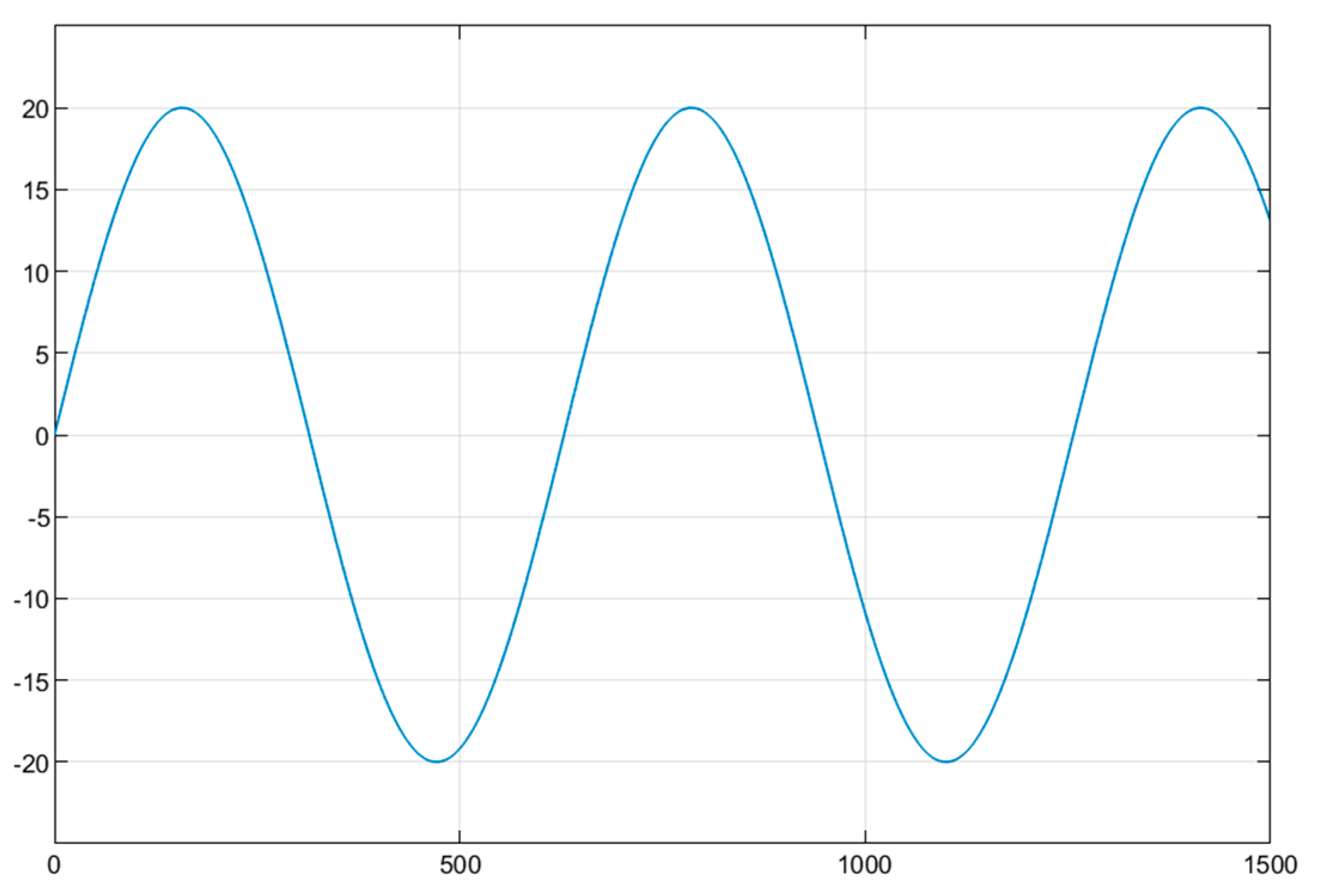
An open-loop simulation system was constructed using Matlab 2023b (Simulink). The simulation duration was set to 200 s, with an identification step h = 0.1 s and an initial motion speed $u_0=2.5 \mathrm{m}/\mathrm{s}$. To ensure the full excitation of the underwater vehicle, a sine function was chosen as the input for the rudder, as depicted in Figure 1.

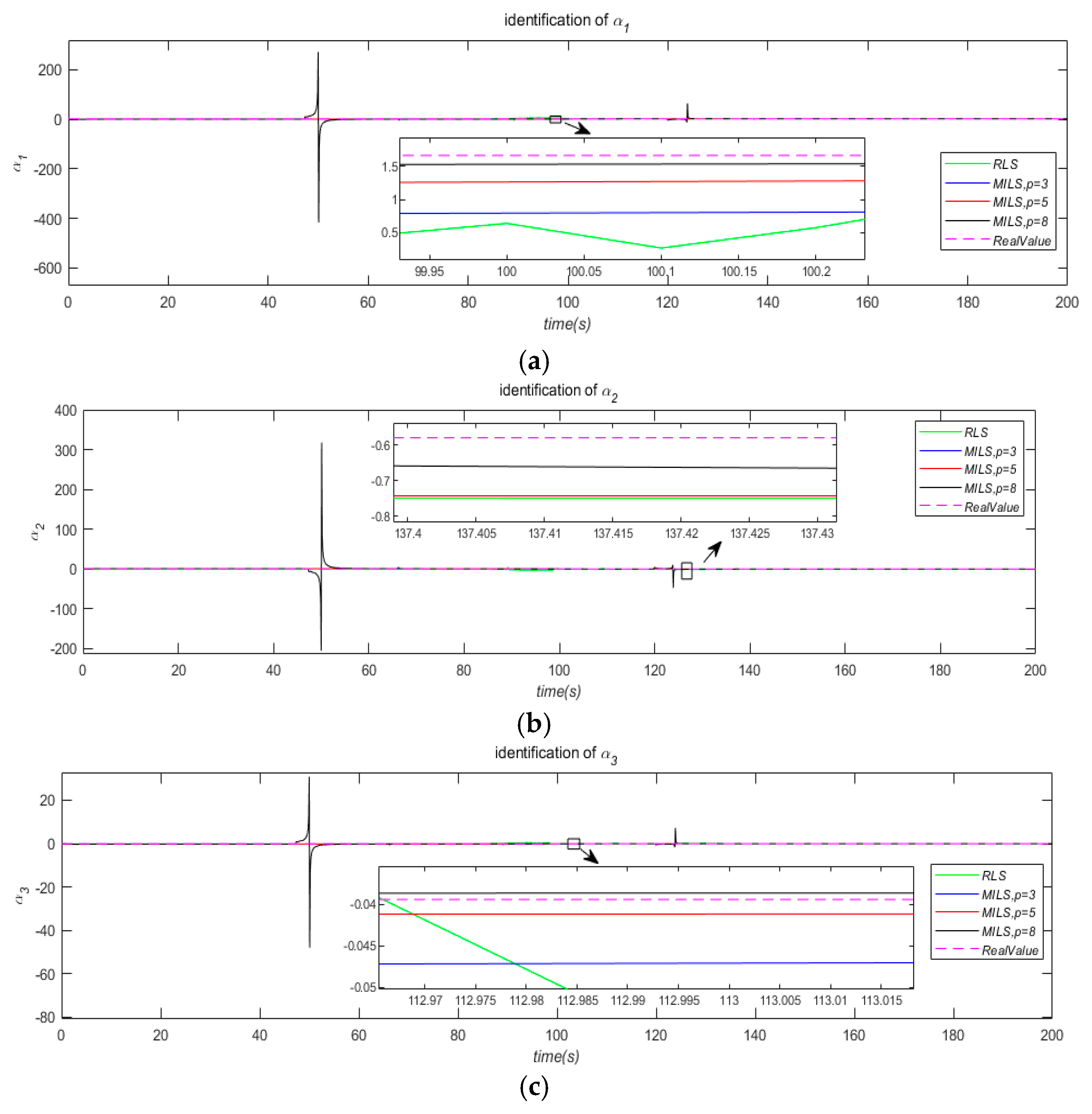
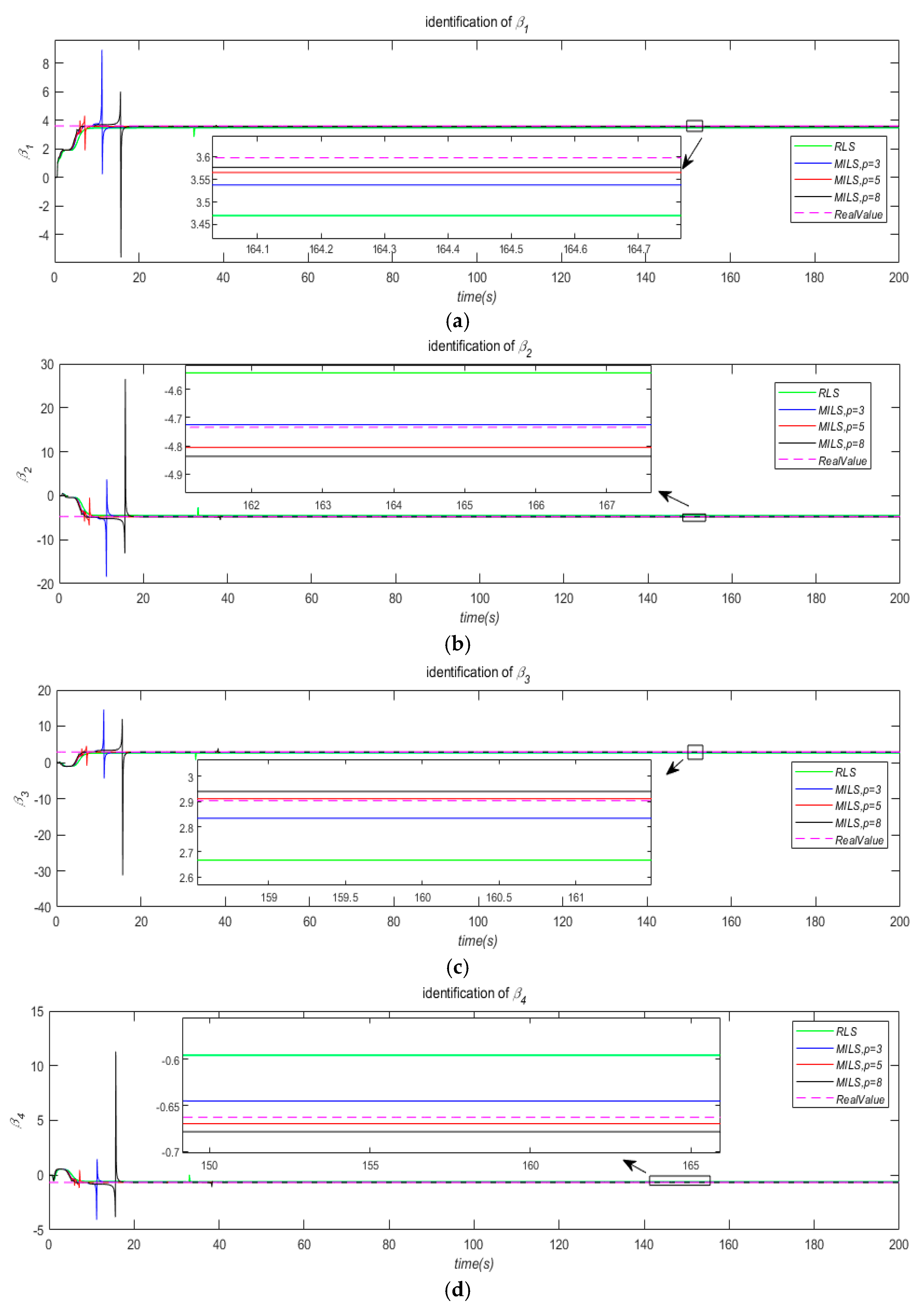
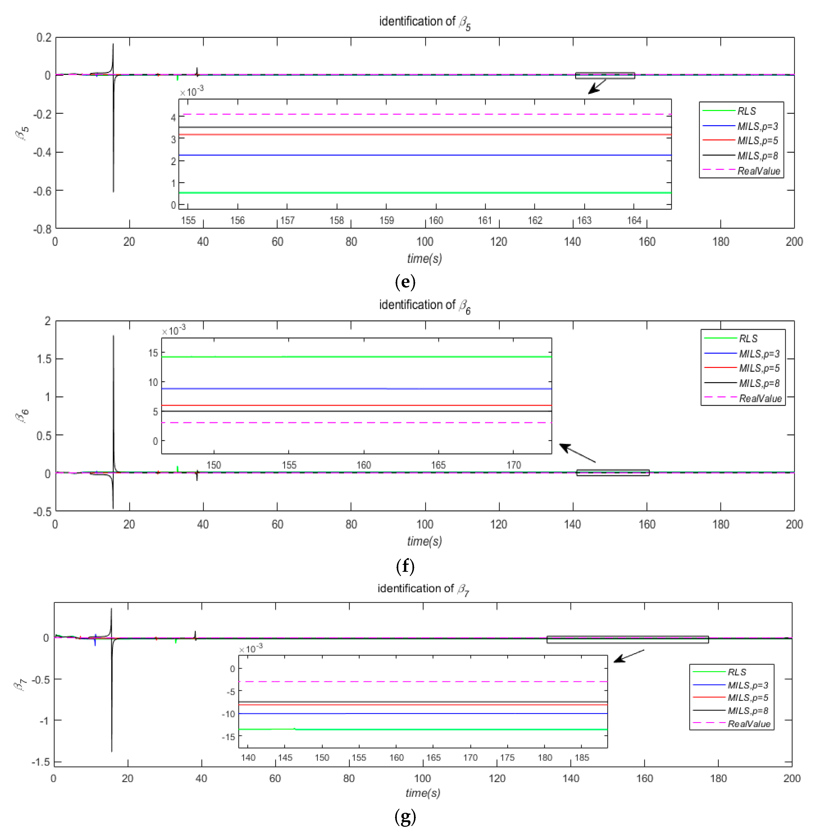
We conducted the parameter identification process based on LS and MILS algorithms, respectively. The estimated value of parameters ${\alpha }_i(i=1,2,3)$ with a time variation curve is shown in Figure 2, Subgraphs abc respectively represent the identification of parameters ${\alpha }_i(i=1,2,3)$. The estimated value of parameters ${\beta }_i(i=1,2,\cdots ,7)$ with a time variation curve is shown in Figure 3, Subgraphs a-g respectively represent the identification of parameters ${\beta }_i(i=1,2,\cdots ,7)$.

The relative estimation error of the parameters is defined as follows:

$$e:={\displaystyle \frac{‖\widehat{\vartheta }-\vartheta ‖}{‖\vartheta ‖}}\times 100\%$$

where e is the error, $\widehat{\vartheta }$ is the estimated parameters, and $\vartheta$ is the real parameters.

Regarding parameters ${\vartheta }_1={\left[\begin{array}{ccc}-{\alpha }_1& -{\alpha }_2& {\alpha }_3\end{array}\right]}^T$, their estimated values and errors based on LS are shown in

Table 2. Estimated values and estimation errors of parameters ${\vartheta }_1={\left[\begin{array}{ccc}-{\alpha }_1& -{\alpha }_2& {\alpha }_3\end{array}\right]}^T$.

$\mathit{t}$	${\mathit{\alpha }}_{\mathbf{1}}$	${\mathit{\alpha }}_{\mathbf{2}}$	${\mathit{\alpha }}_{\mathbf{3}}$	$\mathit{e}$(%)
30	0.2723	0.3123	−0.1997	94.2327
60	0.3639	0.2395	−0.1907	87.6009
100	0.4277	0.1910	−0.1833	83.0437
140	1.6717	−0.7512	−0.0382	9.7860
170	1.6607	−0.7428	−0.0395	9.2928
200	1.6614	−0.7433	−0.0394	9.3207
real value	1.6613	−0.5793	−0.0394	\

, and their estimated values and errors based on MILS (p = 3, 5, 8) are shown in

Table 3. Estimated values and estimated errors of parameters ${\vartheta }_1={\left[\begin{array}{ccc}-{\alpha }_1& -{\alpha }_2& {\alpha }_3\end{array}\right]}^T$ based on MILS.

$\mathit{p}$	$\mathit{t}$	${\mathit{\alpha }}_{\mathbf{1}}$	${\mathit{\alpha }}_{\mathbf{2}}$	${\mathit{\alpha }}_{\mathbf{3}}$	$\mathit{e}$ (%)
3	30	0.2874	0.3009	−0.1979	93.1516
	60	0.5046	0.1323	−0.1745	77.5499
	100	0.7862	−0.0803	−0.1414	57.5356
	140	1.6614	−0.7434	−0.0394	9.3222
	170	1.6613	−0.7433	−0.0394	9.3182
	200	1.6613	−0.7433	−0.0394	9.3182
5	30	0.3029	0.2892	−0.1961	92.0475
	60	0.5228	0.1188	−0.1723	76.2649
	100	1.2546	−0.4352	−0.0868	24.6657
	140	1.6613	−0.7433	−0.0394	9.3177
	170	1.6613	−0.7433	−0.0394	9.3182
	200	1.6613	−0.7433	−0.0394	9.3191
8	30	0.3029	0.2892	−0.1961	90.3457
	60	0.5228	0.1188	−0.1723	72.2974
	100	1.2546	−0.4352	−0.0868	8.6210
	140	1.6613	−0.7433	−0.0394	9.3181
	170	1.6613	−0.7433	−0.0394	9.3182
	200	1.6613	−0.7433	−0.0394	9.3182
real value		1.6613	−0.5793	−0.0394	\

.

The estimated values and errors of parameters ${\vartheta }_2={\left[\begin{array}{ccccccc}-{\beta }_1& -{\beta }_2& -{\beta }_3& -{\beta }_3& {\beta }_5& {\beta }_6& {\beta }_7\end{array}\right]}^T$ based on LS are shown in

Table 4. Estimated values and estimated errors of parameters ${\vartheta }_2={\left[\begin{array}{ccccccc}-{\beta }_1& -{\beta }_2& -{\beta }_3& -{\beta }_3& {\beta }_5& {\beta }_6& {\beta }_7\end{array}\right]}^T$ based on RLS.

$\mathit{t}$	${\mathit{\beta }}_{\mathbf{1}}$	${\mathit{\beta }}_{\mathbf{2}}$	${\mathit{\beta }}_{\mathbf{3}}$	${\mathit{\beta }}_{\mathbf{4}}$	${\mathit{\beta }}_{\mathbf{5}}$	${\mathit{\beta }}_{\mathbf{6}}$	${\mathit{\beta }}_{\mathbf{7}}$	$\mathit{e}$ (%)
5	2.1713	−1.1950	−0.2486	0.2729	0.0077	−0.0029	0.0153	75.53
10	3.4554	−4.4956	2.6199	−0.5797	−0.0003	0.0164	−0.0152	6.03
15	3.4575	−4.5020	2.6264	−0.5819	−0.0002	0.0161	−0.0150	5.89
20	3.4617	−4.5161	2.6414	−0.5871	0.0001	0.0153	−0.0144	5.60
35	3.4694	−4.5397	2.6654	−0.5950	0.0005	0.0142	−0.0136	5.11
50	3.4699	−4.5415	2.6672	−0.5956	0.0005	0.0142	−0.0136	5.08
real value	3.5982	−4.7340	2.9030	−0.5324	0.0041	0.0030	0.0030	\

, and their estimated values and errors based on MILS (p = 3, 5, 8) are shown in

Table 5. Estimated values and estimated errors of parameters ${\vartheta }_2={\left[\begin{array}{ccccccc}-{\beta }_1& -{\beta }_2& -{\beta }_3& -{\beta }_3& {\beta }_5& {\beta }_6& {\beta }_7\end{array}\right]}^T$ based on MILS.

$\mathit{p}$	$\mathit{t}$	${\mathit{\beta }}_{\mathbf{1}}$	${\mathit{\beta }}_{\mathbf{2}}$	${\mathit{\beta }}_{\mathbf{3}}$	${\mathit{\beta }}_{\mathbf{4}}$	${\mathit{\beta }}_{\mathbf{5}}$	${\mathit{\beta }}_{\mathbf{6}}$	${\mathit{\beta }}_{\mathbf{7}}$	$\mathit{e}$ (%)
3	5	2.6753	−2.5112	0.9129	−0.0766	0.0068	−0.0018	0.0086	47.5428
	10	3.4369	−4.4843	2.6402	−0.5928	0.0039	0.0042	−0.0050	6.0478
	15	3.5337	−4.7199	2.8325	−0.6462	0.0026	0.0077	−0.0091	2.2578
	20	3.5402	−4.7350	2.8439	−0.6491	0.0025	0.0081	−0.0096	2.1658
	35	3.5415	−4.7375	2.8455	−0.6495	0.0024	0.0083	−0.0097	2.1531
	50	3.5415	−4.7376	2.8456	−0.6495	0.0024	0.0083	−0.0097	2.1527
5	5	2.6508	−2.4323	0.8288	−0.0469	0.0063	−0.0001	0.0073	49.3521
	10	3.5594	−4.7909	2.8977	−0.6662	0.0032	0.0057	−0.0079	2.2742
	15	3.5656	−4.8056	2.9093	−0.6693	0.0031	0.0061	−0.0083	2.3872
	20	3.5658	−4.8061	2.9096	−0.6693	0.0031	0.0061	−0.0083	2.3902
	35	3.5659	−4.8065	2.9102	−0.6696	0.0031	0.0061	−0.0082	2.3964
	50	3.5662	−4.8073	2.9111	−0.6699	0.0031	0.0060	−0.0082	2.4063
8	5	2.8247	−2.8823	1.2219	−0.1640	0.0058	0.0008	0.0046	39.82
	10	3.5746	−4.8329	2.9365	−0.6781	0.0036	0.0046	−0.0072	2.73
	15	3.5786	−4.8424	2.9439	−0.6801	0.0035	0.0049	−0.0075	2.85
	20	3.5786	−4.8424	2.9439	−0.6801	0.0035	0.0049	−0.0075	2.85
	35	3.5788	−4.8432	2.9449	−0.6805	0.0035	0.0048	−0.0074	2.86
	50	3.5790	−4.8439	2.9457	−0.6808	0.0036	0.0047	−0.0073	2.87
real value		3.5982	−4.7340	2.9030	−0.5324	0.0041	0.0030	0.0030	\

.

Because there are data saturation issues, we set a forget factor with 0.97 at the identification for ${\beta }_i$ with RLS and MILS. Therefore, the convergence speed of ${\beta }_i$ is much faster than ${\alpha }_i$. To avoid affecting the comparison between RLS and MILS, both set the same forget factor.

After analyzing Figure 2 and Figure 3 and Table 2, Table 3, Table 4 and Table 5, the following conclusion can be drawn: the convergence speed based on MILS is significantly faster than that based on RLS, and the identification accuracy of MILS is also higher than that of RLS. Overall, the larger the innovation length p of MILS, the faster the convergence speed and identification accuracy of its algorithm, which will also be correspondingly improved. However the innovation length of MILS is not necessarily better. For example, in Table 5, the identification error of MILS with p = 8 increases compared to p = 5 because a larger innovation length means more complex calculations and is more prone to data saturation. Therefore, in practical applications, it is necessary to flexibly choose a reasonable innovation length.

To further verify the effectiveness of the identification algorithm, as shown in

Table 6. Estimated value of hydrodynamic coefficient.

Parameter		$\frac{Z_w}{m-Z_{\dot{w}}}$	$\frac{M_q}{I_y-M_{\dot{q}}}$	$\frac{M_{\theta }}{I_y-M_{\dot{q}}}$	$\frac{Z_{\delta }}{m-Z_{\dot{w}}}$	$\frac{M_{\delta }}{I_y-M_{\dot{q}}}$	$\mathit{e}$ (%)
real value		−0.6380	−3.3870	−8.1986	0.4139	−3.9412	/
estimated value (RLS)		−1.9136	−3.3864	−8.1972	0.0530	−3.9405	13.1651
estimated value (MILS)	p = 3	−1.1979	−3.3870	−8.1986	0.2414	−3.9412	6.0171
	p = 5	−0.9451	−3.3868	−8.1981	0.3192	−3.9410	3.3011
	p = 8	−0.8215	−3.3870	−8.1986	0.3579	−3.9412	1.9699

, the parameter estimation values shown in Equation (2) can be calculated by the estimated values shown in Table 2, Table 3, Table 4 and Table 5 and Equation (10).

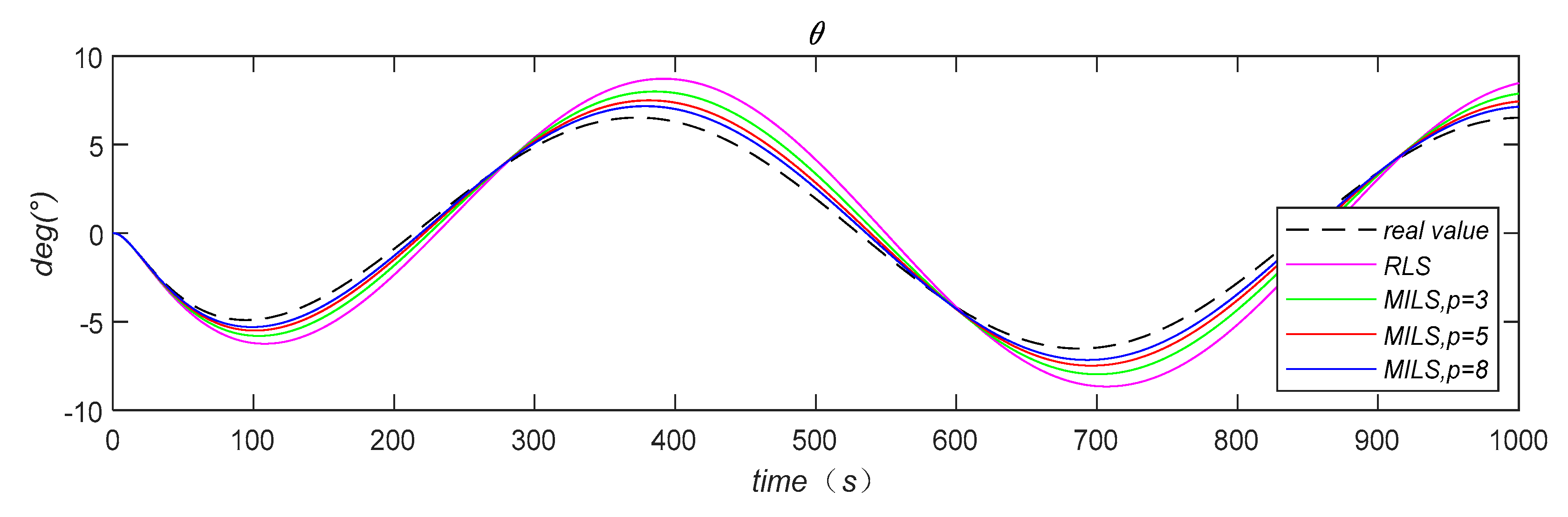
Substituting the estimated values of RLS and MILS shown in Table 4 into Equation (2), using the same sine function shown in Figure 1 as the input rudder, we perform a simulation to obtain the simulated pitch, $\theta$, and depth, $\zeta$, as shown in Figure 4 and Figure 5, respectively.

The estimation error term in Table 6 further confirms that the identification accuracy of MILS is much higher than that of RLS, and the larger the innovation length, the better the identification accuracy. Figure 4 and Figure 5 indicate that compared to RLS, the prediction results based on MILS identification are closer to the true values.

6. Physical Experiments

To further validate the practical applicability of the Multi-Innovation Least Squares (MILS) method in engineering practice, experimental data from full-scale sea trials of an Autonomous Underwater Vehicle (AUV) were utilized to identify a new dynamic model. The dimensions of the AUV’s rudder are shown in

Table 7. Rudder dimension parameters.

Parameter	Value	Unit
Cross-sectional area	4.90 × 10−3	${\mathrm{m}}^2$
Rudder width	6.70 × 10−2	$\mathrm{m}$
Rudder height	7.31 × 10−2	$\mathrm{m}$
Lift coefficient	3.0980	/
Drag coefficient	0.8000	/
Distance from center of gravity	0.7240	$\mathrm{m}$
Maximum rudder angle	13	$\mathrm{degree}(\circ )$

. The motion data were collected during free-run experiments conducted in an external lake [26]. Initially, a low-pass filtering algorithm was applied to the sea trial data to mitigate noise. Subsequently, a first-order model of the AUV’s vertical-plane dynamics was established, and its parameters were identified using the MSLS method. Finally, the identified model was evaluated through closed-loop simulation tests, with the simulated results compared against the measured data to assess model accuracy.

During straight-line motion in the lake, the AUV’s sway velocity remains approximately constant, while the heave velocity and yaw angle exhibit only small-amplitude perturbations. Consequently, higher-order hydrodynamic terms can be neglected, retaining only the first-order hydrodynamic coefficients. Based on the kinematic and dynamic characteristics of the AUV, a linear motion equation in the vertical plane is formulated.

$$\left[\begin{array}{ccc}m-Z_{\dot{w}}& -Z_{\dot{q}}& 0\\ -M_{\dot{w}}& I_{\mathrm{y}}-M_{\dot{q}}& 0\\ 0& 0& 1\end{array}\right]+\left[\begin{array}{ccc}-Z_w& mu-Z_q& 0\\ -M_w& -M_q& 0\\ 0& -1& 0\end{array}\right]\left[\begin{array}{l}w\\ q\\ \theta \end{array}\right]=\left[\begin{array}{c}{Z}_{\delta }\\ M_{\delta }\\ 0\end{array}\right]{\delta }_R$$

(28)

Among them, $Z_{\dot{w}}$, $Z_{\dot{q}}$, $M_{\dot{w}}$, $M_{\dot{q}}$, $Z_w$, $Z_q$, $M_w$, and $M_q$ are the hydrodynamic coefficients to be identified. m and $I_{\mathrm{y}}$ represent the mass of the AUV and the moment of inertia about the Y-axis, respectively, as shown in Table 5. $Z_{\delta }$ and $M_{\delta }$ represent the rudder force coefficient and the rudder moment coefficient, respectively, calculated based on theoretical formulas.

$$Z_{\delta }=-{\displaystyle \frac{1}{2}}\rho A{V}^2{C}_{lr}$$

(29)

$$M_{\delta }=-{\displaystyle \frac{1}{2}}\rho A{V}^2{C}_{lr}{x}_R$$

(30)

Here, ρ denotes the density of the lake water, A is the rudder wing’s cross-sectional area, V is the cruising speed, $C_{lr}$ is the lift coefficient, and $x_R$ represents the distance from the rudder to the coordinate origin.

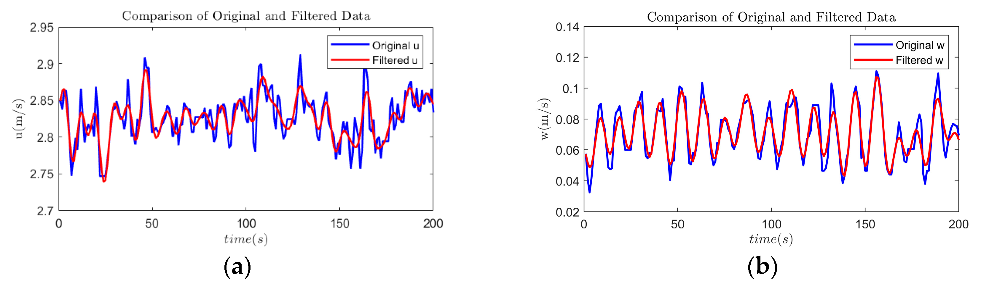
Considering that the measurement data contain noise, a noise term, $n(k)$, is added to the right-hand side of the equation. Accordingly, the identification model established based on the identification algorithm can be expressed as

$$y_1(k)={\phi }_1^T(k){\theta }_1+n(k)$$

(31)

$$y_2(k)={\phi }_2^T(k){\theta }_2+n(k)$$

(32)

where

$$\begin{array}{l}{y}_2(k)=\dot{w}(k),{\phi }_2^T(k)=[\begin{array}{cccc}\dot{q}(k)& w(k)& q(k)& Z_{\delta }{\delta }_R(k)\end{array}]\\ {\theta }_2=[\begin{array}{cccc}{\displaystyle \frac{Z_{\dot{q}}}{m-Z_{\dot{w}}}}& {\displaystyle \frac{Z_w}{m-Z_{\dot{w}}}}& {\displaystyle \frac{Z_q}{m-Z_{\dot{w}}}}& {\displaystyle \frac{1}{m-Z_{\dot{w}}}}\end{array}]\end{array}$$

During the data sampling process, limitations in sensor measurement accuracy and disturbances caused by underwater water flow inevitably lead to data loss and the presence of outliers. As a result, the measured data contain significant noise interference. After removing outliers and corrupted data points, a low-pass filtering method is applied to further process the sampled data, effectively minimizing noise interference. The variables before and after noise reduction are illustrated in Figure 6.

In the previous chapter, parameter identification for the underwater robot was carried out in a simulation environment, demonstrating the effectiveness and feasibility of the proposed Multiple Innovation Least Squares (MILS) algorithm. Building on this, the present chapter applies the MILS method to actual sea trial data from the AUV to further investigate parameter identification, with the aim of validating the MILS algorithm’s effectiveness in real-world underwater robot parameter estimation. During the identification process, an innovation length of p = 8 was selected. The resulting parameter estimates are presented in Figure 7.

After a certain number of iterations, the identification results of the hydrodynamic parameters converge to stable values. However, due to the complex noise interference inherent in the sea trial data, the convergence rate of parameter identification based on actual sea trial data is notably slower than that based on simulation data, and future work will focus on employing advanced filtering techniques and optimizing experimental conditions to improve convergence rates.

To verify the accuracy and effectiveness of the identified hydrodynamic coefficients, the coefficients were incorporated into the AUV’s linear motion equation in the vertical plane. Using this motion model, simulations of maneuvering motions in the horizontal plane were performed. To ensure reliable validation, the control inputs used in the simulations were kept consistent with those recorded in the sea trial data. The prediction results are shown in Figure 8, and the final error calculations are recorded in

Table 8. Experimental result error.

Error	w	θ	q
MILS(MAE)	0.043538	0.44549	0.001001
RLS(MAE)	0.15484	0.5104	0.0014849
MILS(MSE)	0.0027253	0.2779	1.52 × 10−6
RLS(MSE)	0.033808	0.41676	3.72 × 10−6

.

7. Conclusions

This article derives a Controlled Auto Regressive (CAR) model based on the simplified vertical motion of an Autonomous Underwater Vehicle (AUV). Parameter identification leveraging this CAR model significantly reduces the measurement information required from the AUV. Traditional parameter identification methods typically rely on extensive measurement data such as velocity, angular velocity, and acceleration, which depend heavily on the onboard sensors. However, these sensors may be unavailable or prone to substantial measurement errors. By contrast, the proposed CAR model-based approach enables parameter identification using only the AUV’s depth position, pitch attitude measurements, and rudder inputs—three types of information that are considerably easier to obtain. This approach decreases dependency on complex sensor suites and broadens the applicability of parameter identification methods for underwater vehicles. To validate the feasibility of the proposed method and improve the accuracy and convergence speed of parameter estimation, Recursive Least Squares (RLS) and Multi-Innovation Least Squares (MILS) algorithms were employed. The simulation results confirmed the effectiveness of the CAR model-based approach, with the MILS algorithm demonstrating superior identification accuracy and faster convergence compared to RLS. Furthermore, the algorithm, validated with data from free-running physical experiments, effectively captures the hydrodynamic characteristics of the AUV. This study provides valuable practical insights for the manipulation and adaptive control of underwater vehicles.