Design and Performance Study of a Magnetic Flux Leakage Pig for Subsea Pipeline Defect Detection

Abstract

Subsea pipelines, operating in high-pressure and high-salinity conditions, face ongoing risks of leakage. Pipeline leaks can pollute the marine environment and, in severe cases, cause safety incidents, endangering human lives and property. Regular integrity inspections of subsea pipelines are critical to prevent corrosion-related leaks. This study develops a magnetic flux leakage (MFL)-based pig for detecting corrosion in subsea pipelines. Using a three-dimensional finite element model, this study analyzes the effects of defect geometry, lift-off distance, and operating speed on MFL signals. It proposes a defect estimation method based on axial peak-to-valley values and radial peak spacing, with inversion accuracy validated against simulation results. This study establishes a theoretical and practical framework for subsea pipeline integrity management, providing an effective solution for corrosion monitoring.

1. Introduction

Subsea pipelines, vital for global energy transport, operate in high-pressure, high-salinity environments with complex geometries, rendering them prone to corrosion-induced defects, such as cracks and pitting [1]. These defects impair pipeline integrity, potentially causing environmental pollution and economic losses [2]. Thus, effective nondestructive evaluation (NDE) techniques are critical for ensuring operational safety and extending service life.

In-line inspection (ILI) technology is fundamental to pipeline integrity management, widely used for safety assessments and maintenance of energy transport pipelines, utilizing methods like magnetic flux leakage (MFL), ultrasonic testing, eddy current testing, CCTV, and radiographic testing [3,4,5]. Among these, MFL detection, a mature and reliable NDE technique, is widely used to detect and characterize pipeline defects via magnetic field perturbations [6,7]. The theoretical basis of MFL detection originates from Maxwell’s equations, established by James Clerk Maxwell in 1865, which elucidated electromagnetic principles and laid the foundation for MFL technology [8]. In 1966, Zastsepin et al. developed the magnetic dipole model, establishing the relationship between defects and MFL fields and enabling analytical solutions for defect-induced magnetic fields [9]. Mandal et al. later validated the magnetic dipole model’s accuracy experimentally and analyzed MFL field distributions under circumferential stress on pipeline surfaces [10]. As research advanced, techniques like the mirror method and numerical methods for solving MFL fields were developed. In 1975, Hwang et al. pioneered the use of the finite element method to analyze MFL fields, studying the effects of defect length and depth on MFL signals, a major breakthrough in MFL technology [11]. Recently, due to rising pipeline accident rates, researchers globally have extensively studied MFL using the finite element method. Coramik et al. employed ANSYS Maxwell 18 to analyze how crack geometry, magnetization speed, and sensor position affect MFL signals, optimizing detector speed and sensor placement using a custom PIG testing system [12]. Keshwani et al. used 3D finite element analysis to examine how defect surface angle, orientation, and interactions affect MFL signals, estimating defect sizes through a database [13]. Moreover, signal processing research has advanced significantly. Piotrowski et al. used wavelet analysis to reduce MFL signal noise, confirming that continuous wavelet coefficients can identify defect location and size [14]. Mukherjee et al. developed an adaptive channel equalization algorithm for MFL signal preprocessing, reconstructing defect signals to ease subsequent denoising [15].

In addition to MFL and other established NDE methods, transient test-based techniques (TTBTs) have emerged as a promising approach for fault detection in subsea pipelines. TTBTs leverage transient pressure wave analysis to identify anomalies such as leaks and blockages, offering advantages in detecting dynamic changes in pipeline conditions. Meniconi et al. (2024) demonstrated the efficacy of TTBTs in assessing the Trieste subsea pipeline, using transient tests to detect faults and optimize field testing protocols [16,17]. These studies highlight TTBTs’ potential to complement MFL by providing insights into hydraulic anomalies, although their application to corrosion defect characterization remains less explored compared to electromagnetic-based methods like MFL.

As MFL technology matured, diverse detection systems were developed for pipeline defect signal acquisition [18]. The Rosen Group (Germany) developed a high-resolution MFL detector with a sensor array, enabling precise identification of internal corrosion defects, as shown in Figure 1. Kim et al. designed a compact spider-type MFL detector for small-scale operations, employing an Arduino MEGA microcontroller and A1321 Hall sensors to collect magnetic field signals, with feasibility validated via simulations and experiments [19]. Xin et al. developed a high-precision, low-magnetic-force crack detection method using SMSE technology for micro-defects, creating a system with a PC, data acquisition card, and probe, capable of detecting 0.3 mm-wide cracks [20]. Guo et al. designed a triaxial high-definition MFL in-line detector using an ARM-STM32 chip, with reliability confirmed via pull-through experiments [21]. The Piao team at Tsinghua University developed an in-line inspection pig integrating a magnetization device, electrical sensors, a recording system, and an explosion-proof battery, enabling simultaneous measurement of 160-channel triaxial MFL and 80-channel PEC signals [22].

Despite advances in MFL detection for in-line inspections, existing studies primarily analyze single defect types, neglecting the combined effects of multiple factors in complex subsea pipeline conditions. This study tackles the diversity and detection challenges of corrosion defects in subsea pipelines by developing a high-sensitivity MFL pig. It systematically evaluates the effects of defect geometry, excitation strength, sensor lift-off distance, and operating speed on MFL signals using 3D finite element simulations and experimental validation. Additionally, it proposes a defect size inversion method based on axial peak-to-valley values and radial peak-to-peak spacing. This work clarifies the dynamic distribution characteristics of MFL signals, offering an accurate and efficient detection technology for subsea pipeline integrity management and establishing a robust theoretical and experimental foundation for intelligent pig development.

2. Theoretical Basis of Magnetic Flux Leakage Detection

2.1. Principles of In-Line Magnetic Flux Leakage Detection

Subsea pipelines, typically constructed from ferromagnetic materials with high magnetic permeability, utilize this property in magnetic flux leakage (MFL) detection technology [23]. When the excitation device magnetizes the pipeline to saturation, a smooth inner wall allows magnetic flux lines to distribute evenly, parallel to the wall, forming a closed magnetic circuit [24]. However, defects on the inner wall reduce the cross-sectional area, lowering local magnetic permeability and increasing magnetic reluctance, which distorts the magnetic field and generates leakage flux. As shown in Figure 2c, when magnetic flux lines from a permanent magnet encounter a defect, most continue parallel to the pipe wall beneath it, while a small portion leaks into the surrounding air, bypassing the defect before re-entering the wall [25]. This magnetic field, formed by leaking flux lines, is termed the magnetic flux leakage (MFL) field. Magnetic sensors detect and convert MFL field signals, which a data processing system analyzes to evaluate waveforms, enabling the assessment of inner wall damage and completion of pipeline integrity inspections [26].

2.2. Theoretical Calculation Methods for Magnetic Flux Leakage Fields

The finite element method (FEM) is used to model magnetic flux leakage (MFL) fields, providing high computational accuracy and flexibility, especially for creating effective mathematical models of complex defect geometries [27]. Finite element solutions for defect-induced MFL fields are derived from Maxwell’s equations: a cylindrical coordinate system (r, θ, z) is adopted, where z corresponds to the pipeline-axial direction, encompassing Gauss’s law for electricity, Gauss’s law for magnetism, Faraday’s law of electromagnetic induction, and Ampere’s circuital law.

Gauss’s law:

$$\nabla \times D=\rho$$

(1)

Gauss’s law for magnetism:

$$\nabla \times B=0$$

(2)

Faraday’s law of electromagnetic induction:

$$\nabla \times E=-{\displaystyle \frac{\partial B}{\partial t}}$$

(3)

Ampere’s circuital law:

$$\nabla \times H=J+{\displaystyle \frac{\partial D}{\partial t}}$$

(4)

According to the Helmholtz theorem, the vector magnetic potential A is introduced, allowing the magnetic flux density B to be expressed as:

$$B=\nabla \times A$$

(5)

The relationship between the magnetic flux density B and the vector magnetic potential A is given by:

$$B=\nabla \times A$$

(6)

Based on the geometric characteristics of oil and gas pipelines, a cylindrical coordinate system (r, θ, z) is used to derive the governing equations:

$${\displaystyle \frac{1}{\mu }}\left\{{\displaystyle \frac{\partial }{\partial r}}\left[{\displaystyle \frac{1}{r}}{\displaystyle \frac{\partial }{\partial r}}\left(rA\right)\right]+{\displaystyle \frac{\partial }{\partial z}}\left({\displaystyle \frac{\partial A}{\partial z}}\right)\right\}=-J$$

(7)

Using Equation (7), the radial component B_r and axial component B_z of the magnetic field strength are obtained, respectively.

$$B_r=-{\displaystyle \frac{\partial A}{\partial z}}$$

(8)

$$B_z={\displaystyle \frac{1}{r}}{\displaystyle \frac{\partial }{\partial r}}\left(rA\right)$$

(9)

3. Numerical Model Development

A 3D finite element simulation model for magnetic flux leakage (MFL) detection was developed for subsea pipeline applications, systematically evaluating the effects of defect characteristics, excitation strength, lift-off distance, and operating speed on MFL signals.

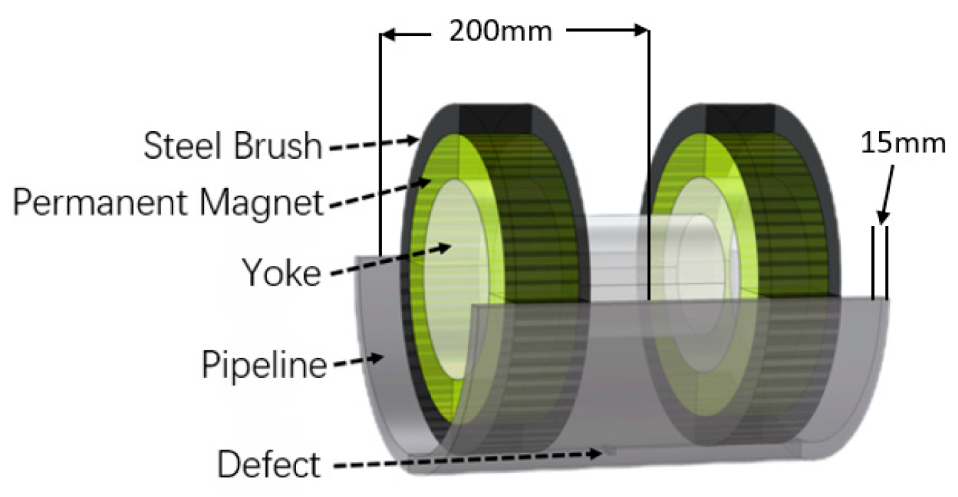
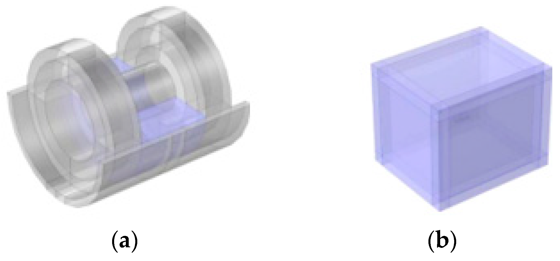
3.1. Establishment of the Geometric Model

Using magnetic flux leakage (MFL) detection principles, a finite element analysis model was developed for subsea pipeline defect detection, evaluating the MFL pig’s performance, as illustrated in Figure 3. The model includes three components: the excitation device, the defective pipeline under inspection, and the surrounding air domain. The pipeline under inspection has an inner diameter of 200 mm and a wall thickness of 15 mm. The excitation device consists of a steel brush, a permanent magnet, and a yoke, with the permanent magnet acting as the excitation source, using axial magnetization to fully magnetize the pipeline for static magnetic field analysis in MFL detection.

In the finite element model, the material properties of the excitation device and pipeline are crucial for accurate numerical calculations. Accordingly, the material properties of the air domain, excitation device (comprising the permanent magnet, yoke, and steel brush), and pipeline were defined based on their physical characteristics. The permanent magnet’s magnetization strength, yoke’s magnetic permeability, steel brush’s magnetic conductivity, and pipeline material’s hysteresis characteristics were parameterized using experimental data and industry standards. The model also incorporated defect geometries, such as crack depth and width, to simulate the effects of typical subsea pipeline damage on MFL signals. The finite element analysis used a static magnetic field solution to calculate MFL field distribution, verifying the pig’s detection sensitivity and reliability across various defect conditions.

3.2. Material Property Definition

The air domain primarily includes the gap between the magnetization device and the pipeline, along with the simulation model’s air enclosure. To ensure computational accuracy and alignment with subsea pipeline conditions, the air domain’s boundary is set to ten times the solution region, as illustrated in Figure 4. The air domain’s material property is defined as air, with a relative magnetic permeability of 1.

To optimize magnetization, the excitation device and pipeline are made from high-permeability materials. The excitation device uses high-performance neodymium–iron–boron (Nd2Fe14B) permanent magnets, the steel brush employs moderately permeable 10# steel, and the yoke and pipeline are made from high-permeability ferromagnetic materials, namely industrial pure iron and 20# steel, respectively [28]. The B-H curves of the materials are defined based on experimental data and industry standards, as shown in Figure 5. The permanent magnet’s coercivity is distinguished into HcB (normal coercivity, the x-intercept on the B-H curve) for magnetic circuit calculations and HcJ (intrinsic coercivity, the x-intercept on the J-H curve) for assessing demagnetization resistance. For the Nd2Fe14B magnet used here, HcB is the primary parameter in defining the excitation strength, while HcJ ensures material stability under operating conditions. Specifically, the permanent magnet exhibits a typical hysteresis loop characteristic of hard magnetic materials, while the yoke and steel brush feature high-permeability curves typical of soft magnetic materials, thereby ensuring magnetic saturation. The accurate definition of these material properties ensures reliable magnetic field distribution calculations in the finite element model, supporting MFL pig performance validation for subsea pipeline defect detection [29].

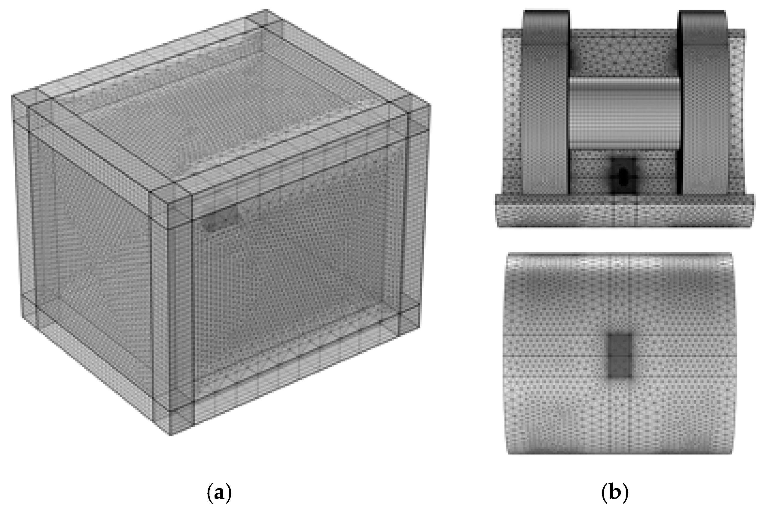
3.3. Mesh Generation

This study employs a static, current-free magnetic field, applying global magnetic flux conservation boundary conditions to ensure consistent magnetic field distribution. The yoke, steel brush, and pipeline’s magnetic behavior is defined by nonlinear B-H curves, while the permanent magnet excitation source uses axial magnetization with a magnetic field strength of ±938,000 A/m along the z-axis, forming a closed magnetic circuit. This configuration ensures stable magnetic flux leakage (MFL) signals for subsea pipeline defect detection.

To improve finite element analysis accuracy, the model uses a regional manual meshing strategy, integrating swept and free tetrahedral meshing, with refined meshing applied to the defect region and its overlying air domain. Meshing results for the air domain are shown in Figure 6a, and refined meshing results for the MFL model and its defect region are depicted in Figure 6b.

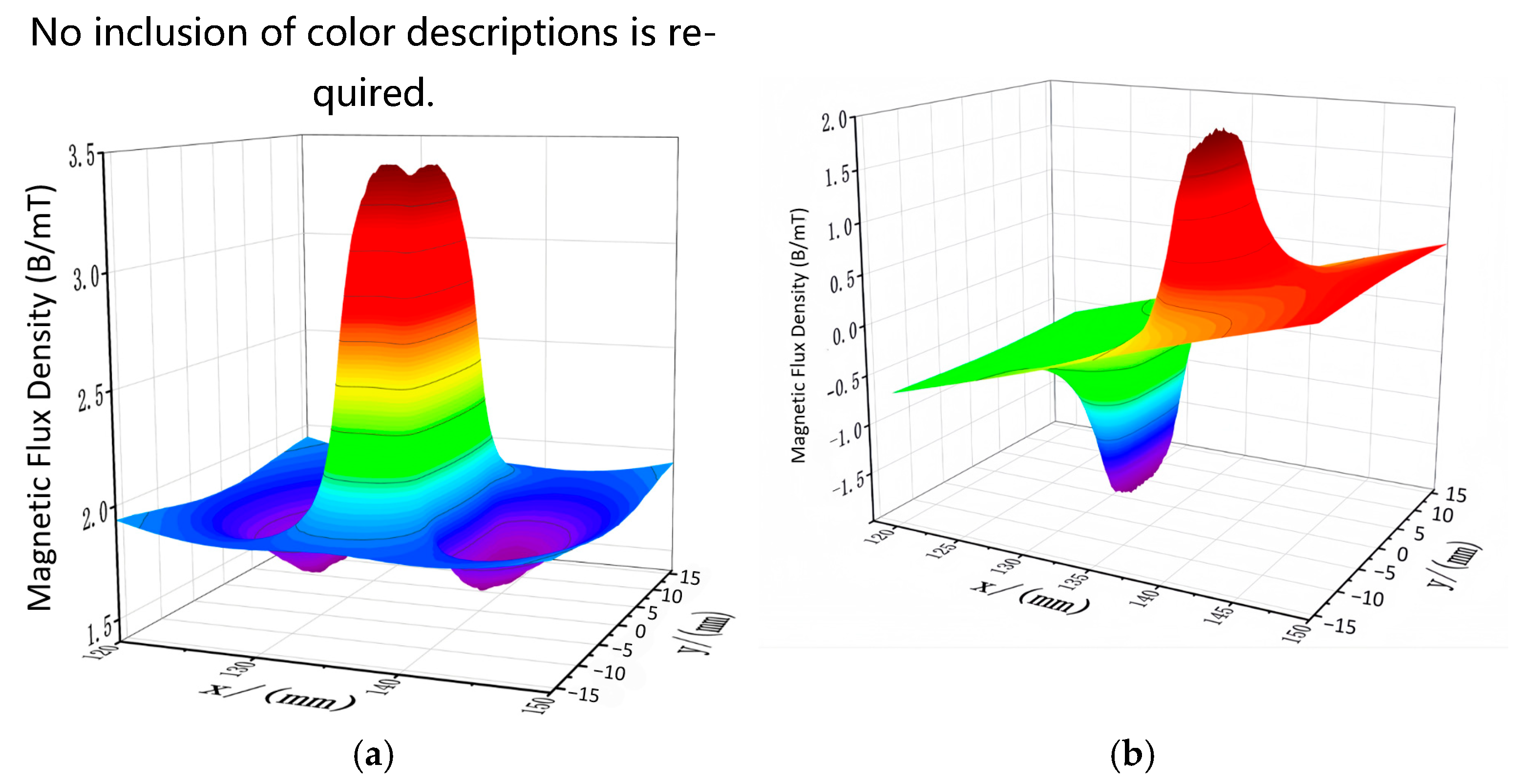
4. Analysis of Defect-Induced Magnetic Flux Leakage Field Distribution Characteristics

Figure 7 shows the volumetric magnetic flux density distribution cloud map for the simulation model. Analysis indicates that magnetic flux lines are concentrated in the pipeline defect region, with peak magnetic flux density at the defect site. To characterize the leakage field’s magnetic flux density distribution above the defect, this study defined a rectangular region (30 mm × 32 mm) 1 mm above the defect, producing 2D cloud maps of the MFL field’s axial and radial components, as shown in Figure 8. Figure 9 shows that the MFL field’s axial and radial components exhibit symmetric distributions about the defect centerline. The axial component features a dual-peak, dual-valley structure, with peaks at the defect center and valleys at its edges, consistent with axial symmetry, while the radial component has a single peak and valley of equal amplitude, showing central symmetry.

Simulation results show that defect geometry and size, excitation device magnetization strength, magnetic sensor height, and detector operating speed significantly influence MFL signal detection. Using the established 3D MFL finite element simulation model, this study will systematically evaluate the effects of these four factors on MFL signals at pipeline defects, analyze their distribution characteristics, and provide theoretical and practical guidance for optimizing MFL pig design and improving subsea pipeline integrity detection.

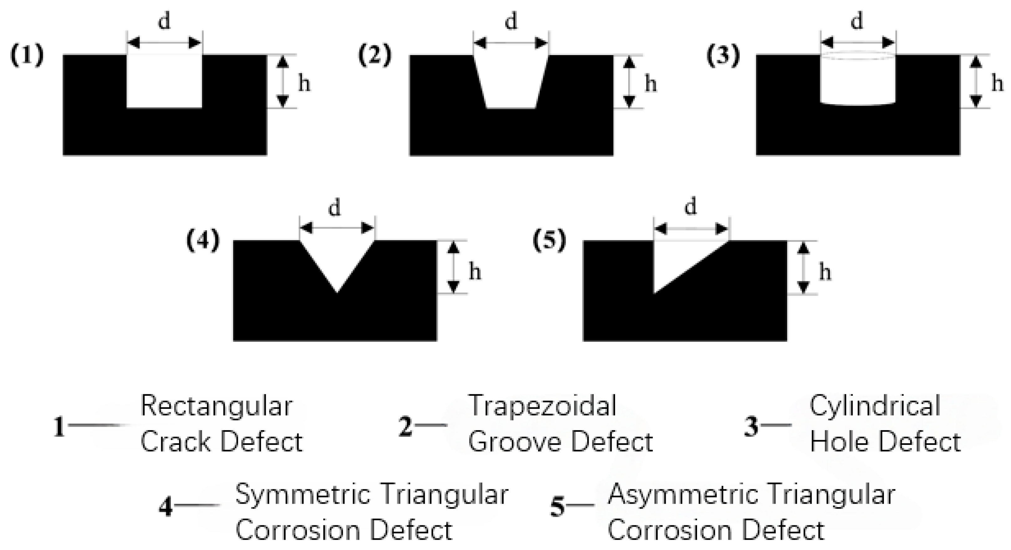
4.1. Influence of Defect Geometry on Magnetic Flux Leakage Signals

4.1.1. Defect Shape

Subsea pipelines, exposed to prolonged corrosion in marine environments, develop surface defects of diverse shapes and sizes, such as cracks, dents, holes, and symmetric or asymmetric corrosion [30]. To enable finite element simulation, this study simplified the geometry of various defect types, as shown in Figure 10. By systematically varying defect shapes in the simulation model while keeping defect depth, width, and simulation conditions constant, this study analyzed the effects of shape variations on MFL signal distribution characteristics.

Figure 11 shows 2D cloud maps of the MFL field’s axial and radial component signal distributions in a region 1 mm above various defect types. Analysis reveals that, regardless of defect type, the MFL field’s magnetic flux density concentrates at defect edges, with peak field strength, allowing axial MFL field cloud maps to clearly outline each defect’s geometric contours. For symmetric defect shapes (e.g., rectangular, cylindrical, symmetric trapezoidal, symmetric triangular), the MFL field’s axial component shows axial symmetry about the defect centerline, while the radial component exhibits central symmetry about the defect center. For asymmetric triangular defects, however, the MFL field’s magnetic flux density deviates from these patterns, showing non-standard distribution characteristics.

To evaluate the effect of defect shape variations on MFL field magnetic flux density, this study defined a 40 mm line segment 1 mm above the defect, simulating MFL signals captured by magnetic sensors as the detector passes over it. Figure 12 shows the variations in axial and radial MFL signal strength for different defect shapes. Analysis indicates that, under consistent detection conditions, rectangular defects yield the highest MFL signal strength, widest waveform width, and largest amplitude variation, whereas symmetric triangular defects produce the lowest signal strength, narrowest waveform width, and smallest amplitude variation. Cylindrical and trapezoidal defects differ in MFL signal strength but have similar waveform widths. For asymmetric triangular defects, the axial and radial MFL signal peaks exhibit significant offsets, deviating from typical axial and central symmetry, consistent with prior analysis. However, the reduced distance between asymmetric triangular defect boundaries and the excitation device prevents signal attenuation, resulting in a higher MFL signal peak than that of symmetric triangular defects.

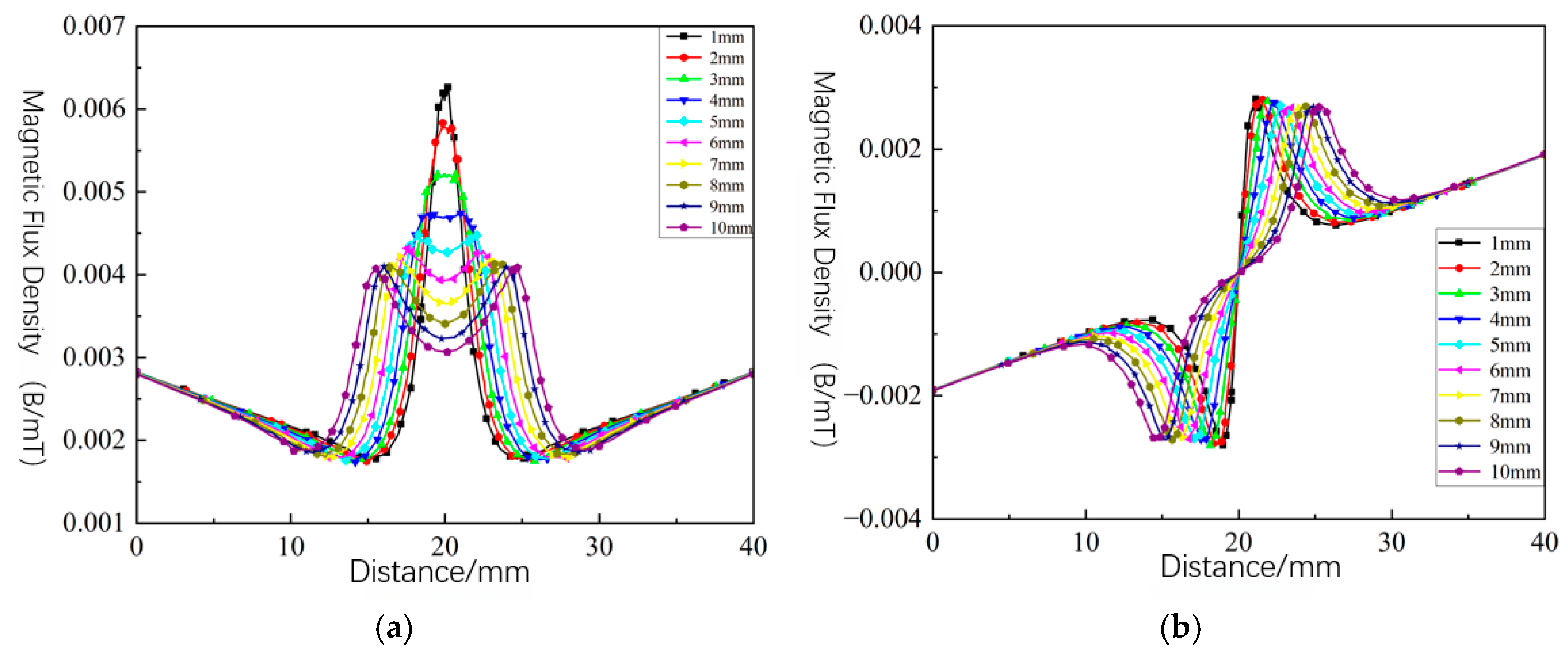
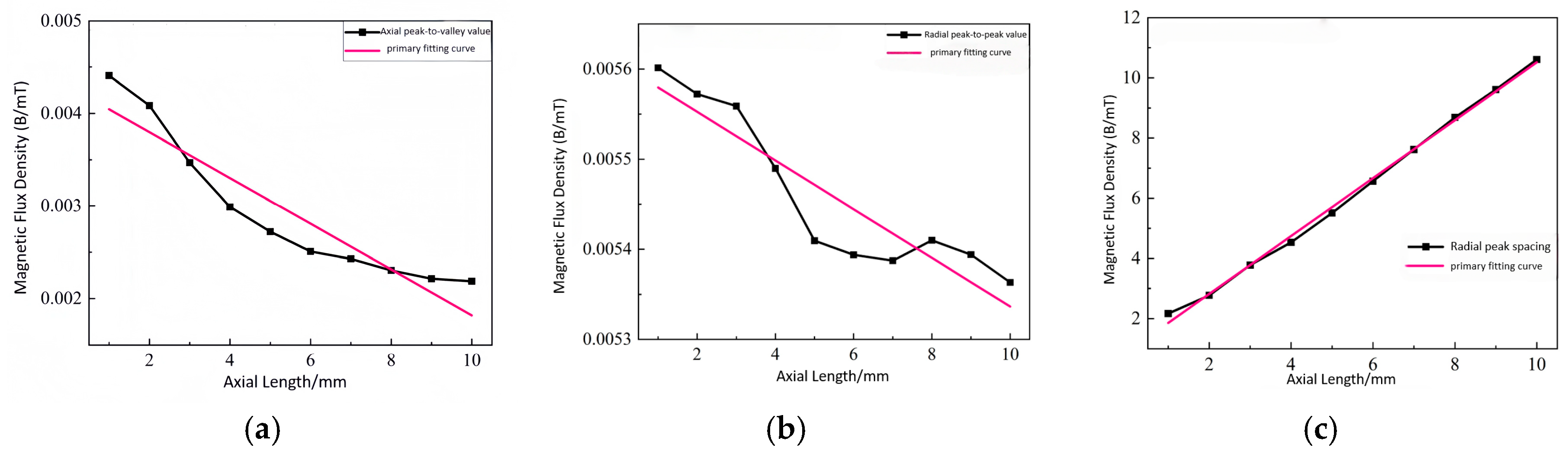
4.1.2. Defect Longitudinal Length

As rectangular defects yield the strongest magnetic flux leakage (MFL) signals and most significant simulation results, this section examines their axial length and radial depth variations’ effects on MFL signals. With defect width constant and depth at one-third of the pipeline wall thickness, axial length was increased from 1 mm to 10 mm in 1 mm increments. Figure 13 shows the axial and radial MFL field component distributions. Analysis reveals that the axial component signal peak decreases with increasing axial length, while waveform width increases. At an axial length of 4 mm, the axial component signal curve shifts from a single-peak to a dual-peak structure. The radial component peak decreases with increasing axial length, while peak-to-peak spacing increases.

The axial peak-to-valley value, radial peak-to-peak value, and radial peak-to-peak spacing are key parameters for analyzing MFL signal distribution and defect quantification, with variation trends shown in Figure 14. The axial peak-to-valley value is the difference between the peak and valley in the axial signal curve, the radial peak-to-peak value is the difference between dual peaks in the radial signal, and the radial peak-to-peak spacing is the distance between these peaks. As noted earlier, the MFL field concentrates at defect edges, making radial peak-to-peak spacing a critical parameter for inverting defect longitudinal length. To accurately describe these parameters’ variation patterns, this study performed a fitting analysis of their variation curves. Figure 14 indicates that the simulated radial peak-to-peak spacing slightly exceeds the actual defect longitudinal length but follows a linear variation trend. Thus, radial peak-to-peak spacing is a key parameter, supporting accurate quantification and inversion of subsea pipeline defect longitudinal length.

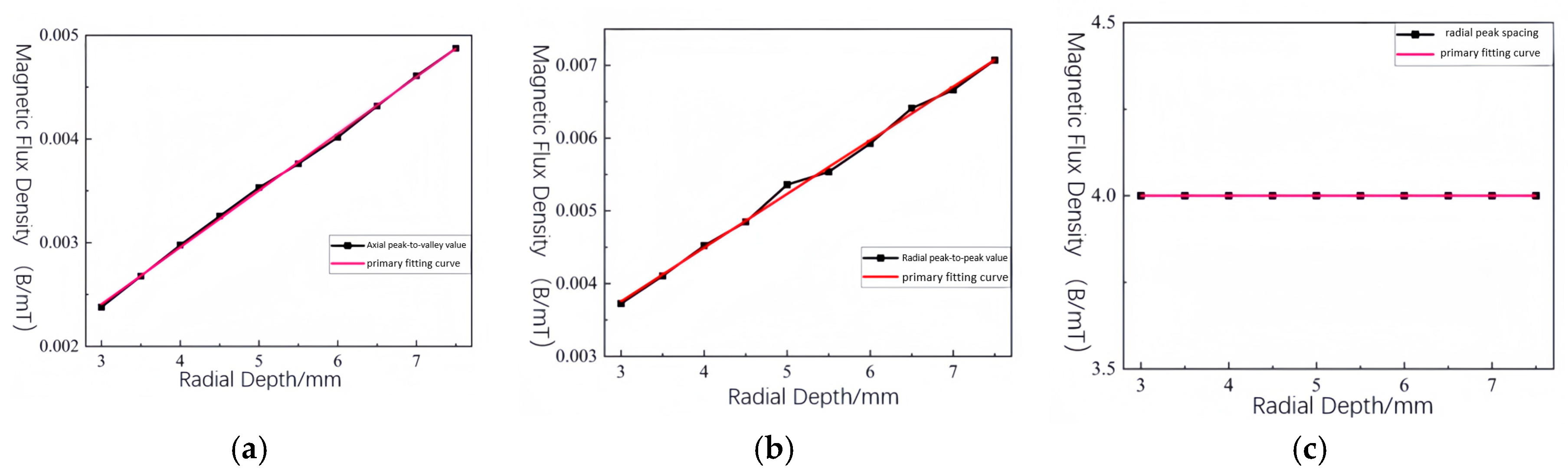
4.1.3. Defect Radial Depth

This study examines the effect of varying radial depth from 3 mm to 7.5 mm in 0.5 mm increments on magnetic flux leakage (MFL) signal distribution, using a rectangular defect with a constant 3 mm axial length and fixed width. Figure 15 and Figure 16 show the variation trends of the MFL field’s axial and radial components and three parameters: axial peak-to-valley value, radial peak-to-peak value, and radial peak-to-peak spacing. Analysis indicates that increasing defect depth linearly increases the axial peak-to-valley value and radial peak-to-peak value, while radial peak-to-peak spacing remains unchanged. Fitting results confirm that the axial peak-to-valley value and radial peak-to-peak value are linearly and positively correlated with defect depth. Thus, analyzing the axial peak-to-valley value and radial peak-to-peak value enables accurate defect depth determination, supporting reliable defect quantification.

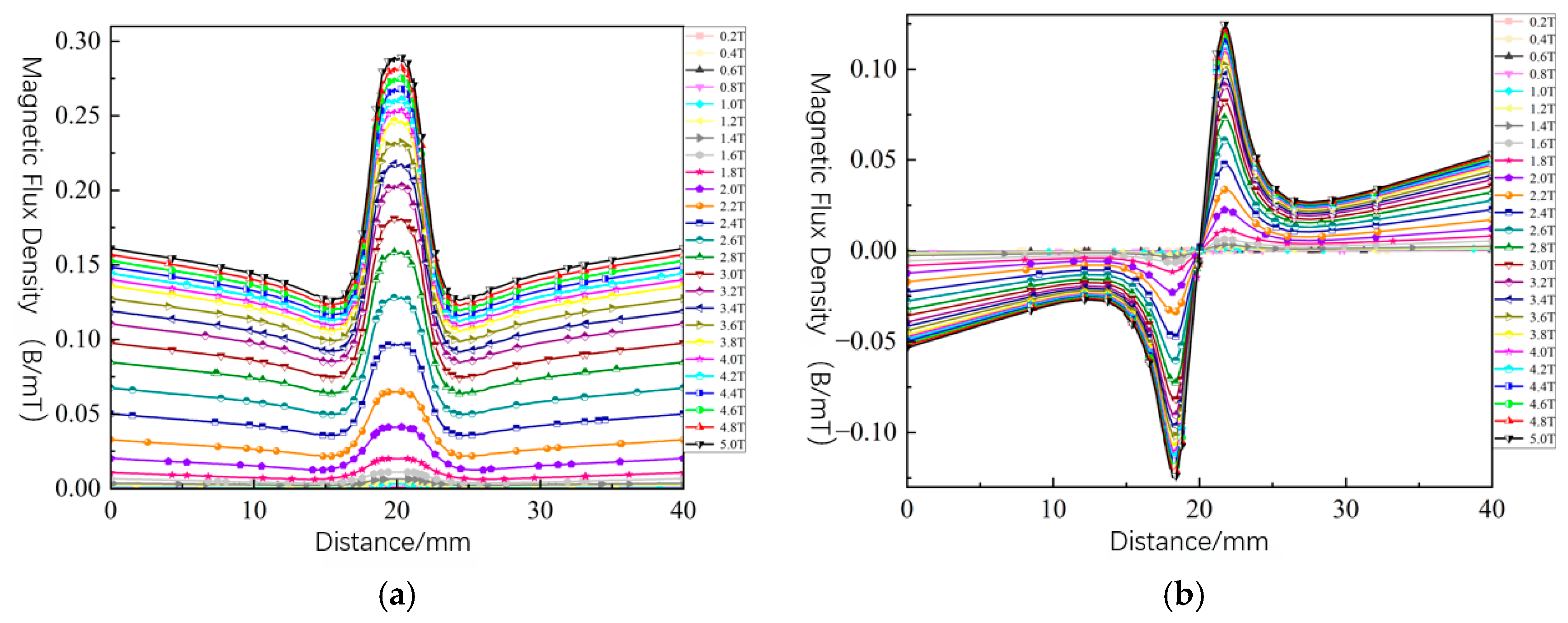
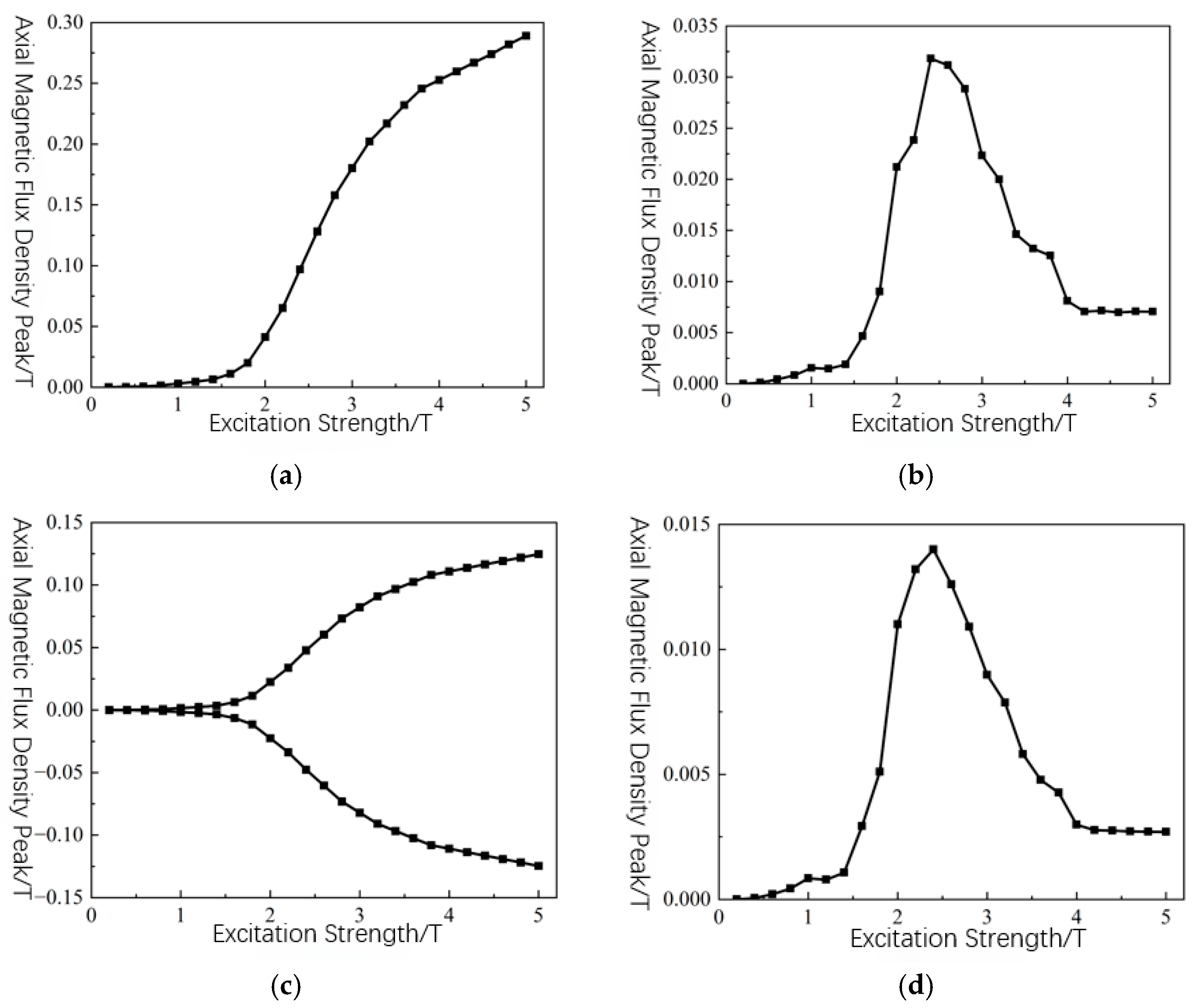
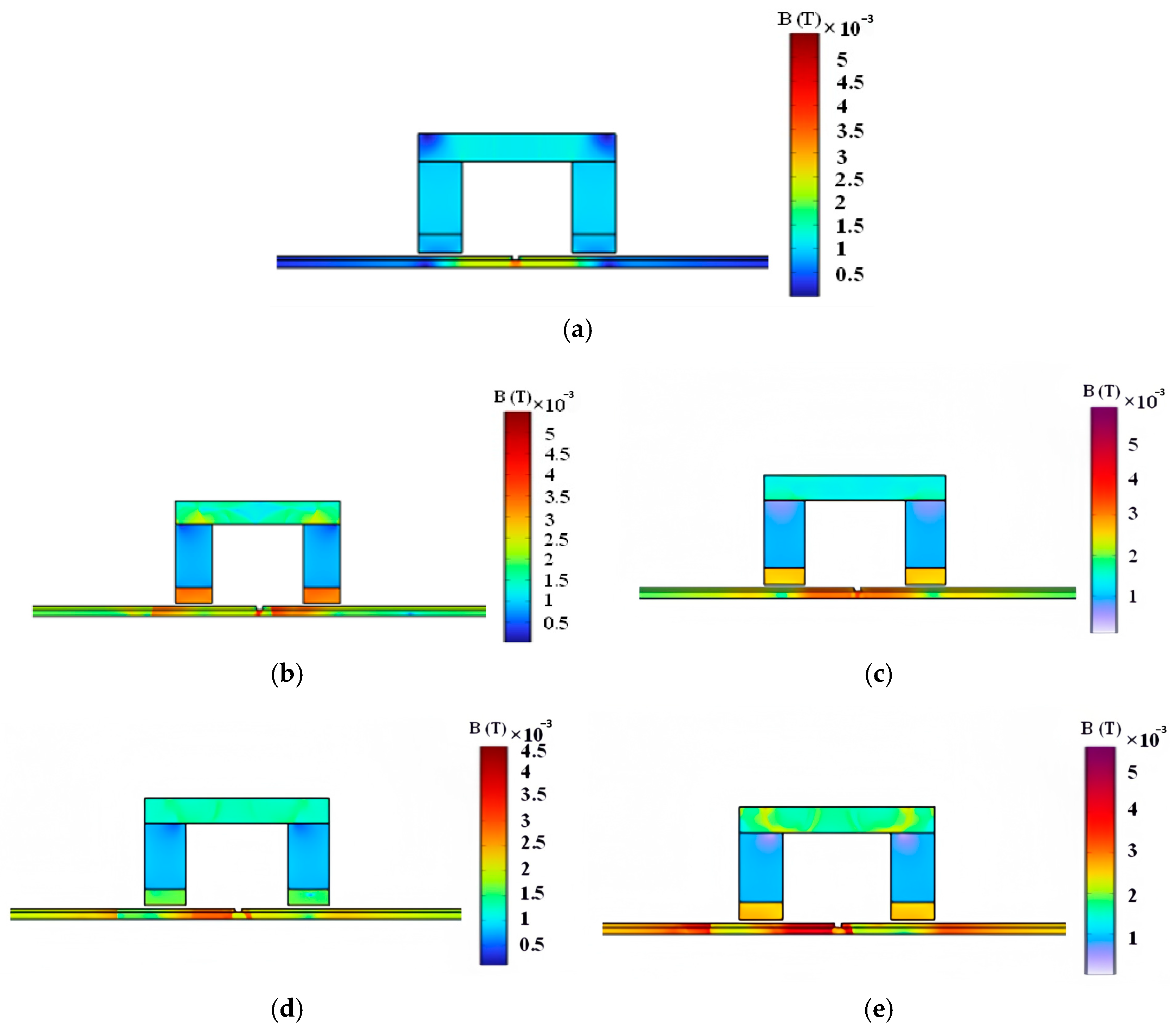
4.2. Regulation of Magnetic Leakage Signals by Excitation Intensity

To evaluate the detection performance of a magnetic flux leakage (MFL) pig under subsea pipeline operating conditions, this study examines the effect of excitation intensity on MFL signal strength using a forward modeling approach. While practical permanent magnets like NdFeB are limited to coercivities rarely exceeding 2 T due to material properties, this study extends the simulation range to 5.0 T for theoretical purposes, allowing an examination of saturation trends beyond current technological bounds. HcJ is referenced for material selection to prevent demagnetization, but not varied in simulations. Figure 17 shows the variation curves of the MFL field’s axial and radial component signals under varying excitation intensities, with permanent magnet coercivity increasing from 0.2 T to 5.0 T in 0.2 T increments. Analysis reveals that as excitation intensity increases, the MFL signal strength at the defect site rises, but incremental changes are non-uniform. Figure 18 shows the variation curves of the axial and radial MFL signal peak values with excitation intensity, divided into three stages: initial growth, nonlinear growth, and saturated linear growth. Below 1.2 T, the initial growth stage shows slow MFL signal peak growth with minimal incremental changes; between 1.2 T and 2.4 T, the nonlinear growth stage exhibits rapid peak increases, peaking at 2.4 T; above 2.4 T, the saturated linear growth stage shows continued but slower peak growth, stabilizing at 4.0 T. Thus, the detector’s magnetization device should use moderate excitation intensity. Excessively high excitation intensity enlarges the magnetization device, increasing pipeline operational resistance and risking detector jamming, while excessively low intensity causes insufficient magnetization, hindering effective MFL signal capture by sensors.

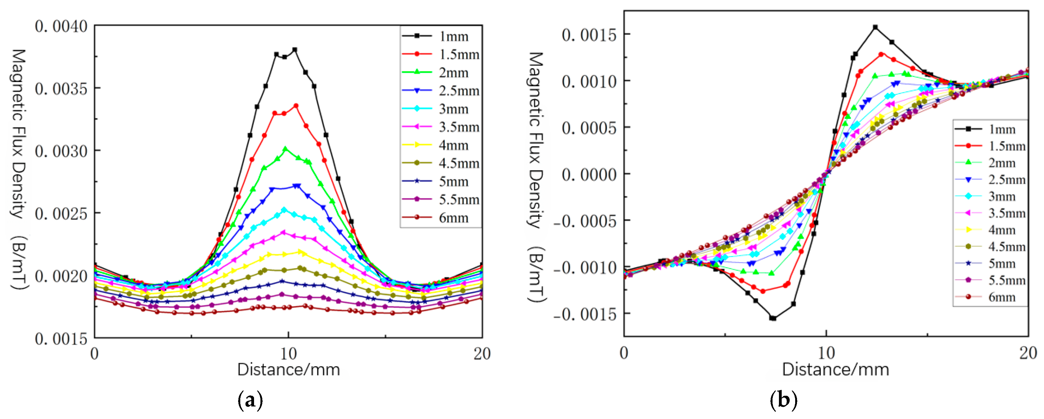
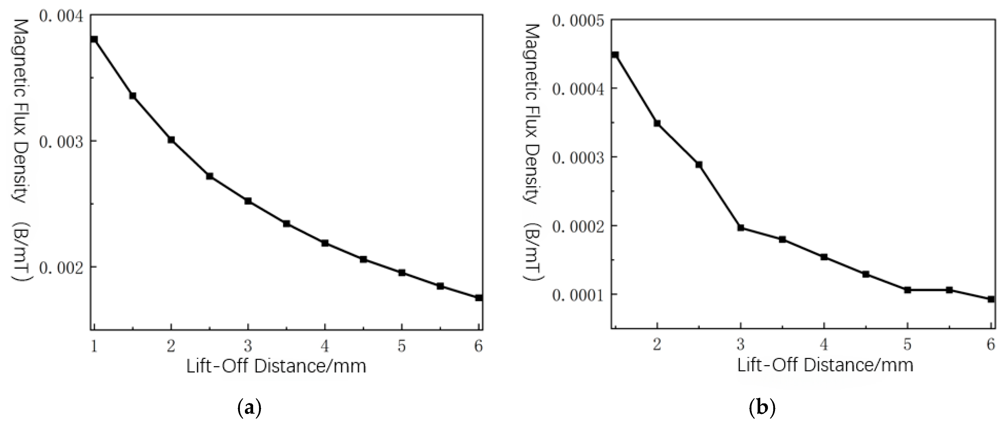
4.3. Sensitivity of Magnetic Leakage Signals to Sensor Lift-Off Value

In subsea pipeline defect detection, surface roughness and defects cause random vibrations during detector operation. The detector’s magnetization device, flexibly connected to the pipeline via steel brushes, experiences negligible vibration effects on the excitation circuit during magnetization. However, the magnetic sensor, typically made of tempered spring steel, is susceptible to random vibrations, causing variations in the sensor-to-pipeline distance (lift-off value). Thus, evaluating the effect of lift-off value variations on magnetic flux leakage (MFL) signal detection is crucial.

This study defines a 20 mm axial detection path above a pipeline surface defect, incrementally adjusting the path-to-defect distance. To enhance probe durability in practice, a wear-resistant pad prevents direct sensor-to-pipeline contact, and the lift-off value is simulated from 1 mm to 6 mm in 0.5 mm increments to analyze the MFL field’s axial and radial component signals. Figure 19 shows that MFL signal strength significantly attenuates with increasing lift-off value, reducing detection accuracy. At a 6 mm lift-off value, the axial and radial MFL signal curves nearly lose peak and valley characteristics, yielding the lowest detection accuracy. Figure 20 shows the variation trend of the axial MFL signal peak value, with Figure 20b indicating that within the 1–3 mm lift-off range, the signal peak value changes most significantly, reducing detection accuracy due to lift-off fluctuations. In the 3–6 mm lift-off range, the signal peak value change stabilizes, suggesting that a higher lift-off value mitigates fluctuation effects on detection accuracy. Based on this simulation, the magnetic sensor lift-off value should be set between 3 and 5 mm to minimize random vibration interference and maintain detection accuracy.

4.4. Dynamic Influence of Operating Speed on Magnetic Leakage Signals

In subsea pipeline inspection, subsea current velocity significantly affects the magnetic flux leakage (MFL) pig’s operating speed, impacting MFL signal detection performance. Thus, evaluating the effects of operating speed variations on MFL signals is essential. Due to the pig’s relative motion with the pipeline, the simulation requires a transient field solution. Transient solutions require substantial computational resources; to reduce this burden and solution time, this study employs a simplified 2D MFL simulation model. The 2D model aligns with the previously described 3D model but uses a flat iron plate of equal thickness instead of the pipeline, retaining identical defect dimensions, permanent magnet, yoke, and steel brush thicknesses, and coercivity settings.

The pig’s operating speeds are set at 0, 1, 2, 3, and 4 m/s. Figure 21 shows the magnetic field distribution cloud map inside the pipeline when the detector reaches the defect center. When stationary above the defect center, the pig produces a uniform magnetic field distribution, symmetric about the defect, with maximum magnetic induction intensity at the defect’s periphery. As the pig moves, the magnetic field distribution becomes perturbed, losing uniformity, with perturbation increasing at higher operating speeds.

Figure 22 shows MFL signals captured by the magnetic sensor at different pig operating speeds when reaching the defect center. Analysis reveals that increasing operating speed intensifies MFL signal distortion, shifting the axial component’s baseline and distribution from a double-peak to a single-peak profile. Increasing operating speed significantly reduces axial and radial MFL signal strength, adversely affecting detection performance. Thus, in engineering applications, higher pig operating speeds require increased excitation strength to enhance subsea pipeline defect detection robustness and minimize missed detections due to low signal strength.

5. Design of the Magnetic Leakage Detection System

Figure 23 illustrates the framework of the magnetic flux leakage (MFL) detection system. To precisely measure MFL signals at defect locations in subsea pipelines, the system uses a magnetization module to fully magnetize the pipeline, producing a strong MFL field at the defect site. The signal acquisition unit captures the MFL signal and converts it into an electrical signal. The conditioning circuit then amplifies and filters the electrical signal to enhance its quality. The processed electrical signal is transmitted to the Arduino development board’s A/D converter for conversion into a digital signal. The digital signal is then stored and visualized on a PC for data analysis.

5.1. Design of the Magnetization Module

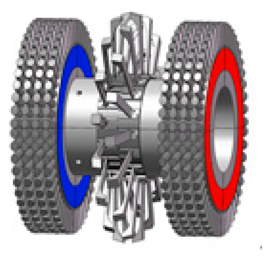
5.1.1. Structural Design

The magnetization module, a critical component of the magnetic flux leakage (MFL) detection system, directly influences detection performance. The magnetization module uses a steel brush-type magnetic circuit structure, comprising permanent magnets, a yoke, and steel brushes, as shown in Figure 24.

Permanent magnets, as the excitation source of the magnetization module, directly influence the magnetic flux leakage (MFL) field strength at defect locations. Due to limited pipeline internal space, permanent magnets are installed on the detector’s outer side with constrained dimensions, as overly small sizes weaken excitation. To address this, the permanent magnets use high-energy-product N52 NdFeB, with performance parameters shown in

Table 1. Performance parameters of N52 permanent magnet.

Remanent Magnetic Induction Intensity		HcB (Normal Coercivity)		HcJ (Intrinsic Coercivity)		Intrinsic Coercivity		Maximum Magnetic Energy Product
Max	Min	Min (kA/m)	Min (kOe)	Min (kA/m)	Min (kOe)	kOe	kA/m	Max	Min
14.8 kGs	14.6 kGs	950	11.5	900	9.6	≥9.6	≥900	52 MGOe	50 MGOe
1.48 T	1.46 T							400 kJ/m3	380 kJ/m3

, distinguishing HcB for circuit reluctance calculations and HcJ for demagnetization resistance. The yoke, serving as a magnetic circuit bridge between the permanent magnets, ensures a uniform and stable magnetic circuit by guiding magnetic flux lines. The yoke requires high-permeability soft magnetic materials, such as industrial pure iron or permalloy, with DT4 industrial pure iron selected for its cost-effectiveness. Steel brushes, in direct contact with the pipeline, provide structural support in the magnetization module and minimize air gap reluctance between the permanent magnets and pipeline via dense steel wires, optimizing magnet performance. The steel brush material must balance high magnetic permeability and moderate mechanical strength; insufficient strength compromises support, while excessive strength increases pipeline wall friction, raising pig operating resistance. After thorough evaluation, the study selects 20# steel for the steel brushes.

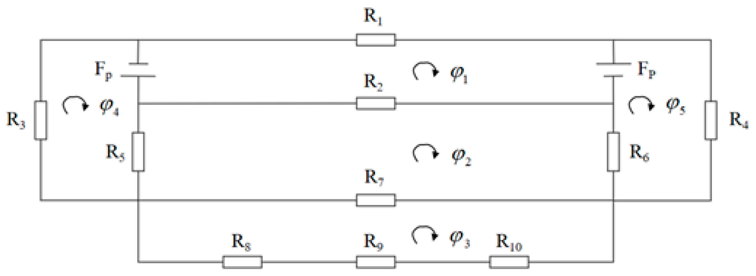
5.1.2. Magnetic Circuit Design

To ensure full pipeline magnetization for optimal magnetic flux leakage (MFL) detection performance, precise magnetic circuit calculations are necessary. This study assumes a defect at the magnetization module’s center and develops an equivalent magnetic circuit model based on its structural characteristics, as shown in Figure 25. To aid analysis, the magnetization module’s parameter symbols are defined in

Table 2. Key parameters of the magnetization device.

Parameter Name	Symbol
Permanent Magnet Length	ly
Permanent Magnet Width	wy
Permanent Magnet Thickness	hy
Steel Brush Thickness	hg
Yoke Thickness	he
Distance Between the Steel Brush on One Side and the Pipeline at the Defect	Lgg
Defect Length	Lq
Defect Width	Wq
Defect Height	Hq
Pipeline Thickness	Hp

.

Magnetic potential of the permanent magnet F_p:

$$F_p=H_c{h}_y$$

(10)

where H_c denotes the coercivity of the permanent magnet.

Internal reluctance of the yoke R₁:

$$R_1={\displaystyle \frac{2L_{gg}+L_q}{{\mu }_e{w}_y{h}_e}}$$

(11)

where μ_e is the magnetic permeability of the yoke.

Reluctance of the air gap between the two magnets R₂:

$$R_2={\displaystyle \frac{2L_{gg}+L_q}{{\mu }_e{w}_y{h}_y}}$$

(12)

where μ₀ is the magnetic permeability of air.

Reluctance of the air gap between the steel brush and the yoke R_ge:

$$R_{ge}=R_3+R_4={\displaystyle \frac{L_{ge1}}{{\mu }_0{S}_{ge1}}}+{\displaystyle \frac{L_{ge2}}{{\mu }_0{S}_{ge2}}}$$

(13)

where L_ge1 and L_ge2 are the air gap lengths at different positions, and S_ge1 and S_ge2 are the cross-sectional areas of the air gaps at different positions.

Reluctance of the steel brushes, R₅ and R₆:

$$R_5=R_6={\displaystyle \frac{h_g}{{\mu }_g{l}_y{w}_y}}$$

(14)

where μ_g is the magnetic permeability of the steel brushes.

Reluctance of the air gap between the steel brushes on both sides, R₇:

$$R_7={\displaystyle \frac{2L_{gg}+L_q}{{\mu }_0{h}_g{w}_y}}$$

(15)

Internal reluctance of the defect-free pipeline segments, R₈ and R₁₀:

$$R_8=R_{10}={\displaystyle \frac{L_{gg}}{{\mu }_p{w}_y{H}_p}}$$

(16)

where μ_p is the magnetic permeability of the pipeline.

Internal reluctance of the pipeline at the defect, R₉:

$$R_9={\displaystyle \frac{L_q}{{\mu }_p\left(w_p{H}_p-w_q{H}_q\right)}}$$

(17)

Based on Kirchhoff’s laws and the above expressions, the following system of equations is derived:

$$\begin{array}{c}\left(R_3+R_5\right){\phi }_4-R_5{\phi }_2=H_c{h}_y\\ \left(R_4+R_6\right){\phi }_5-R_6{\phi }_2=H_c{h}_y\\ \left(R_8+R_9+R_{10}\right){\phi }_3-R_7{\phi }_2=0\\ \left(R_2+R_5+R_6+R_7\right){\phi }_2-R_2{\phi }_1-R_5{\phi }_4-R_6{\phi }_5-R_7{\phi }_3=0\\ \left(R_1+R_2\right){\phi }_1-R_2{\phi }_2=0\end{array}$$

(18)

The thickness of the permanent magnet, h_y, and the cross-sectional area of the magnet in the magnetic circuit, S_y, are, respectively:

$$h_y=K_r{H}_y\left(2L_{gg}+L_q\right)\sqrt{{\displaystyle \frac{B_r}{H_c{\left(BH\right)}_{max}}}}$$

(19)

$$S_y=K_f{B}_x{S}_x\sqrt{{\displaystyle \frac{H_{cb}}{B_r{\left(BH\right)}_{max}}}}$$

(20)

where K_r is the reluctance coefficient, H_y is the magnetic field strength of the permanent magnet, B_x is the magnetic induction intensity of the air between the two magnets, and S_x is the cross-sectional area of the air between the two magnets:

$$K_f={\displaystyle \frac{S_q}{B_g{S}_g\sqrt{\frac{H_{cb}}{B_r{\left(BH\right)}_{max}}}}}$$

(21)

where S_q represents the cross-sectional area of the defect in the magnetic circuit direction, B_g is the magnetic induction intensity of the pipeline, and S_g is the cross-sectional area of the pipeline in the magnetic circuit.

As magnetic permeability (μ) varies nonlinearly with magnetic field strength (H), this study uses a parameter approximation method to solve the model. Based on calculation results and pipeline internal space constraints, the permanent magnet dimensions are set as a 40 × 20 × 10 mm cuboid, meeting magnetization saturation requirements.

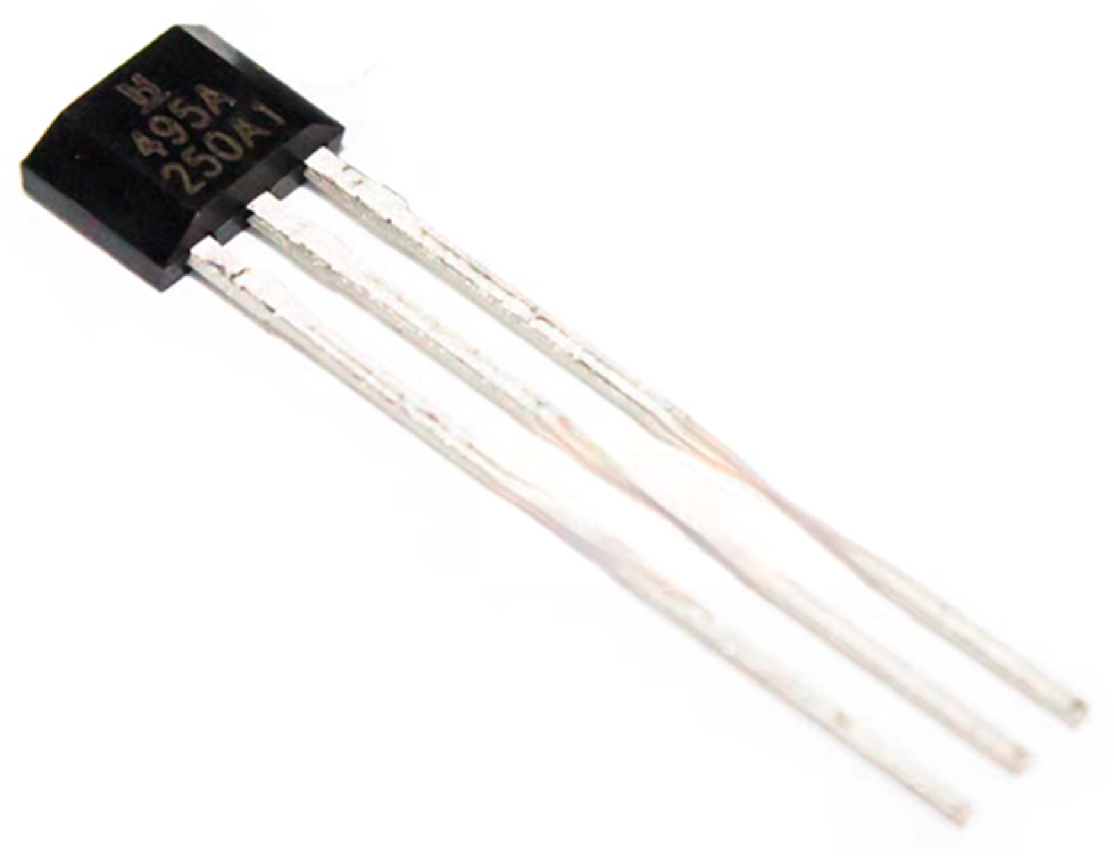
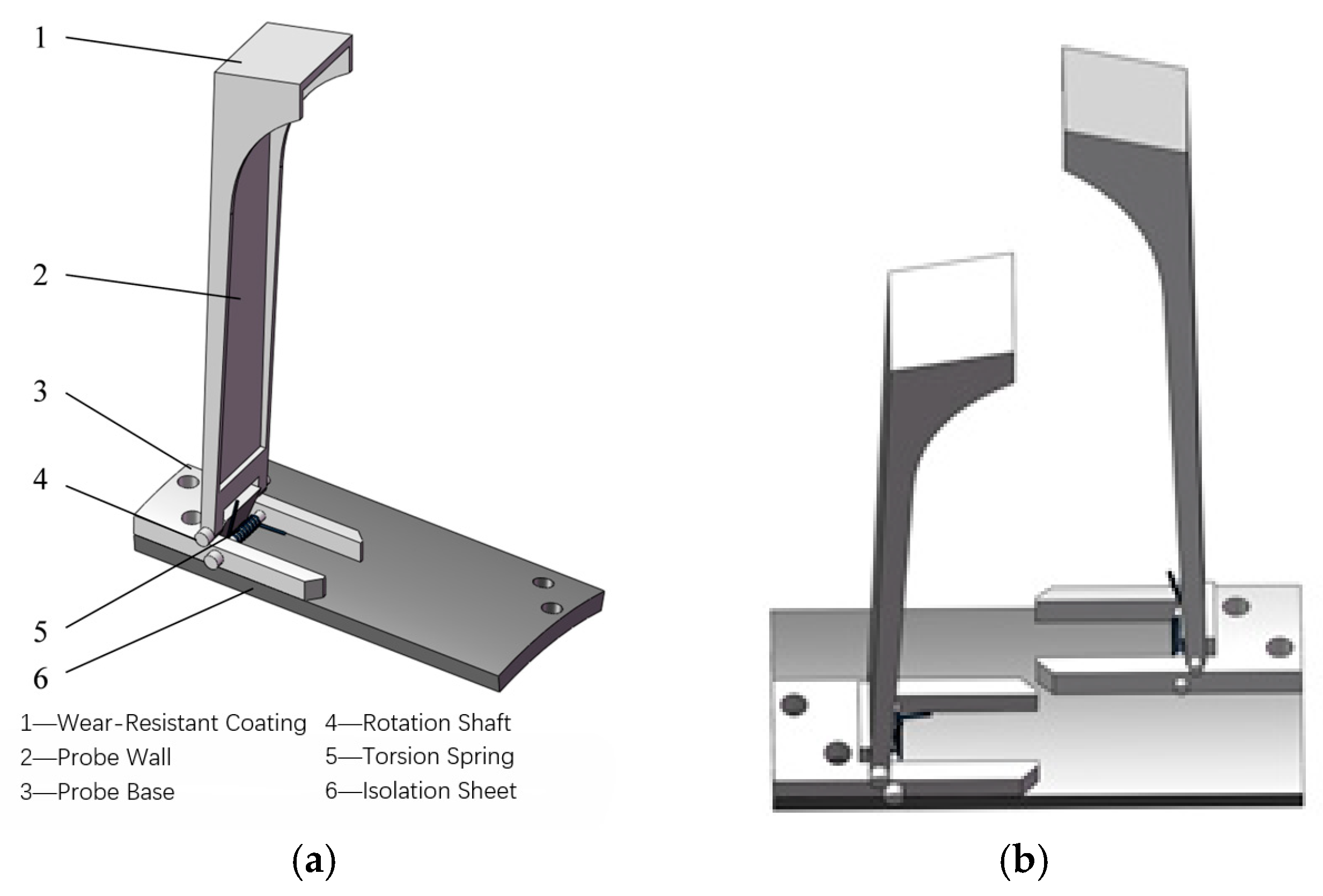
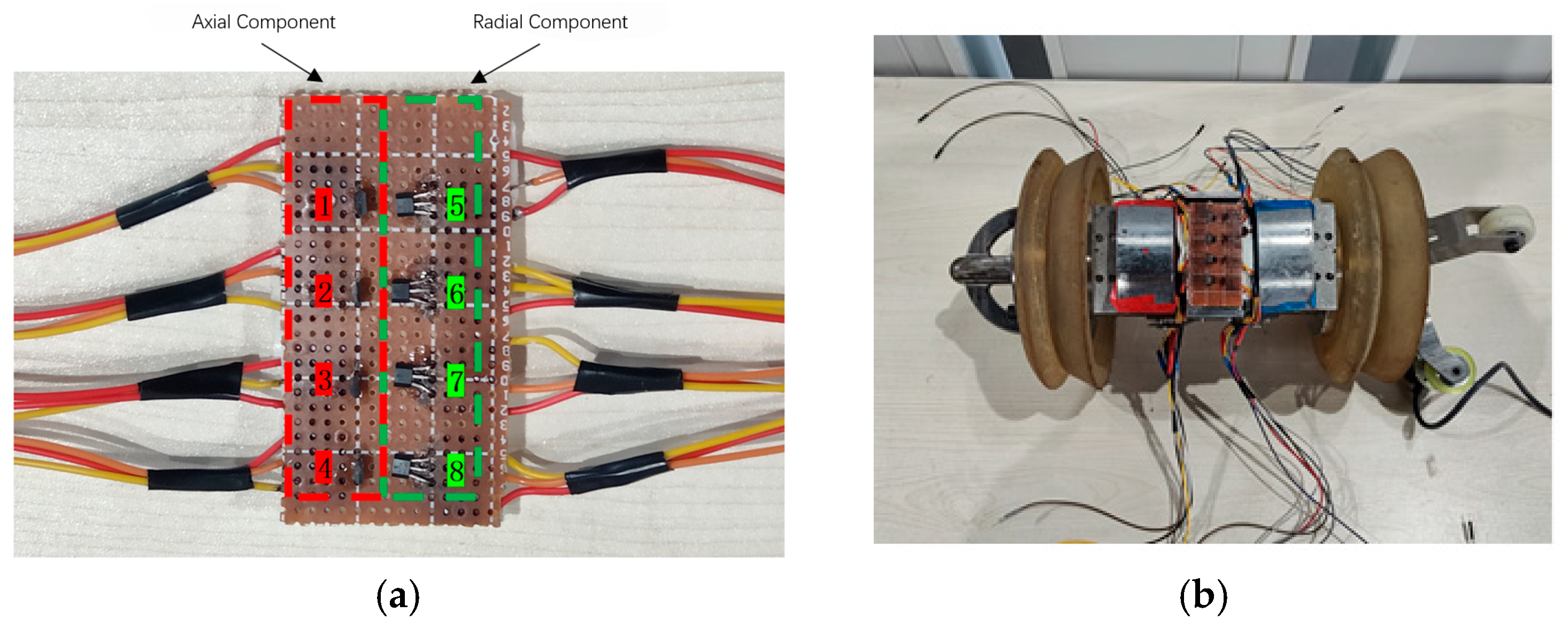
5.2. Development of the Signal Acquisition Module

The signal acquisition module, a critical component of the magnetic flux leakage (MFL) detection system, captures MFL signals at pipeline defect locations and comprises a magnetic sensor, sensor bracket, wear-resistant layer, and associated circuits. The magnetic sensor, mounted between magnetic poles via the sensor bracket, converts MFL signals into electrical signals for transmission and processing.

Various sensors are available for magnetic detection, including induction coils, fluxgate sensors, Hall elements, magnetic diodes, and magnetoresistive sensors. Different sensor types have distinct performance characteristics and applications, requiring the careful selection of sensors for MFL detection based on technical attributes.

Table 3. Comparative analysis of magnetic sensor types.

Magnetic Sensor	Advantages	Disadvantages
Induction Coil	Adjustable measurement sensitivity, sensitive to high-frequency magnetic signals	Highly susceptible to operating speed, complex signal processing
Fluxgate Sensor	Extremely high detection sensitivity	Large space requirement, suitable only for weak magnetic fields
Hall Element	Small space requirement, directly reflects magnetic field strength, unaffected by operating speed	Requires a power supply circuit, relatively high detection sensitivity
Magnetic Diode	Extremely high detection sensitivity	Significantly affected by temperature
Magnetoresistive Sensor	Extremely high detection sensitivity	Suitable only for weak magnetic fields

compares the advantages and limitations of mainstream magnetic sensors.

After evaluating the advantages and limitations of various magnetic sensors, the Hall element is selected for the signal acquisition module in the magnetic flux leakage (MFL) detection system due to its compact size, high stability, and straightforward measurement method. Hall elements are classified into switching and linear types based on application, with linear Hall elements preferred for their high sensitivity. The linear Hall element converts magnetic flux leakage (MFL) signals into voltage outputs, where stronger external magnetic fields yield higher voltages, enabling characterization of MFL field strength at defect locations, as described by the Hall effect equation:

$$V_H=K_{H}IBsin\alpha$$

(22)

In the equation, V_H represents the Hall voltage, I denotes the input current, K_H is the Hall coefficient, B is the magnetic induction intensity, and α is the angle between the Hall element surface and the magnetic field. In a static, zero-magnetic-field environment, the linear Hall element’s output voltage is theoretically 50% of the supply voltage. When exposed to an external magnetic field, the output voltage varies based on the field’s strength and direction.

In the magnetic flux leakage (MFL) detection system design, Honeywell SS490 series linear Hall elements are preferred for their low cost, temperature-stable accuracy, and circuit design flexibility. After comparative analysis, this study selects the SS495A Hall element as the magnetic sensor for the MFL detection system, as shown in Figure 26. The SS495A sensor features three pins (power, ground, signal output) and uses an SMD-DIP3 package, with performance parameters detailed in

Table 4. Parameter table of SS495A hall effect sensor.

Model	SS495A
Dimensions	4 × 3 × 2.5 mm
Operating Voltage	5 V
Linear Range	−67~+67 mT
Sensitivity	3.125 ± 0.125 mV/G
Linearity Error	1.0%
Temperature Error	±0.06% °C

.

Given the compact size and limited range of Hall sensors, a uniform array of sensors is arranged around the detector’s periphery to prevent missed defect detections. The probe bracket positions Hall sensors close to the pipeline wall to minimize lift-off value, ensuring detection accuracy. As shown in Figure 27a, the probe structure uses an integrated design with a probe arm and base connected by a rotating shaft, where a torsion spring ensures close contact with the pipeline wall. To reduce interference from the magnetization device’s magnetic flux lines transmitted through the yoke, a thin non-magnetic nickel–iron alloy layer is placed between the probe base and yoke, providing magnetic isolation to minimize Hall element interference. To maintain detection accuracy, magnetic sensors are positioned close to the pipeline surface, with a wear-resistant coating applied to the probe arm’s contact surface to reduce wear and protect the sensors.

Each probe arm integrates two Hall elements. The SS495A Hall element captures magnetic flux leakage (MFL) signals in a single direction, determined by its orientation. To enable multidirectional MFL signal acquisition, the design places two probe sets between each pair of magnetic poles, as shown in Figure 27b, to capture axial and radial MFL components. Figure 28 shows the assembly structure of the magnetization and detection devices, with the MFL detection system incorporating 32 probe sets and 64 Hall sensors to efficiently capture axial and radial MFL components.

5.3. Integration of the Control System

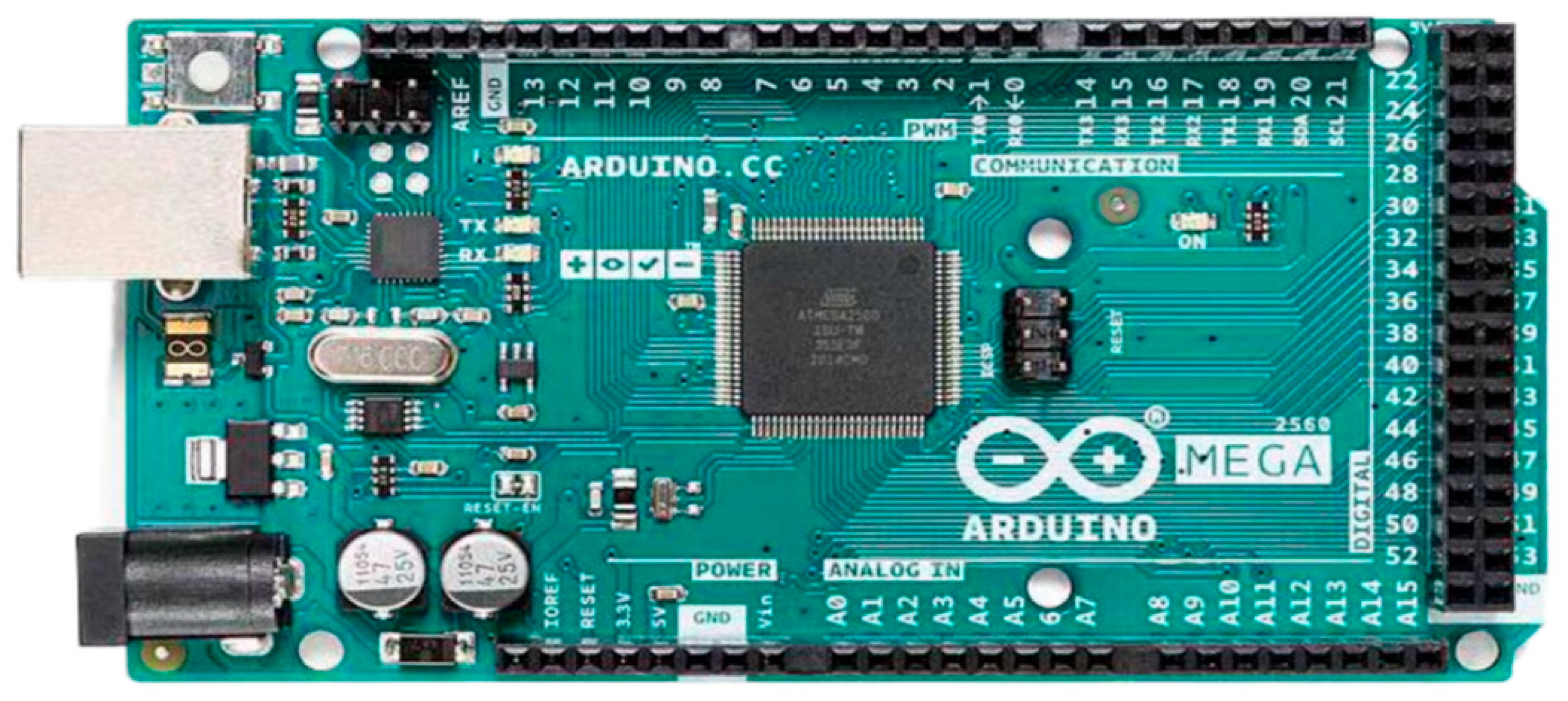
5.3.1. Main Control Chip

The magnetic flux leakage (MFL) detection system uses an Arduino development board as the main control chip. Compared to STM32 series microcontrollers or data acquisition cards used in traditional MFL detection equipment, the Arduino platform provides superior operational simplicity and cost-effectiveness. Traditional microcontrollers (e.g., STM32) require complex configurations, such as pin definitions, output mode selection, voltage level initialization, and port initialization, while Arduino achieves these with a single line of code.

As an open-source electronic prototyping platform, Arduino is preferred for electronic prototype design and interactive projects due to its convenience, flexibility, and open-source nature. The platform includes hardware (Arduino development boards) and software (Arduino IDE version 2.3.2.), with models like UNO, MEGA, and Due offering distinct performance capabilities, enabling selection based on project requirements and cost constraints. The Arduino IDE offers an open-source environment with built-in, callable function libraries, implementing programming logic via setup (initialization) and loop (main loop) functions, ensuring user-friendly operation.

The MFL detection system’s requirement for comprehensive pipeline surface scanning with numerous magnetic sensors necessitates a main control chip with multiple analog I/O interfaces. The Arduino MEGA 2560 (Arduino Inc., Monza, Italy), based on the ATmega2560 microcontroller (Microchip Technology Inc., Chandler, AZ, USA), offers 54 digital and 16 analog I/O interfaces, with configurable pins, enabling multi-channel sensor array integration, as shown in Figure 29. Thus, this study selects the Arduino MEGA 2560 as the core control module for the MFL detection system to meet multi-channel signal acquisition requirements.

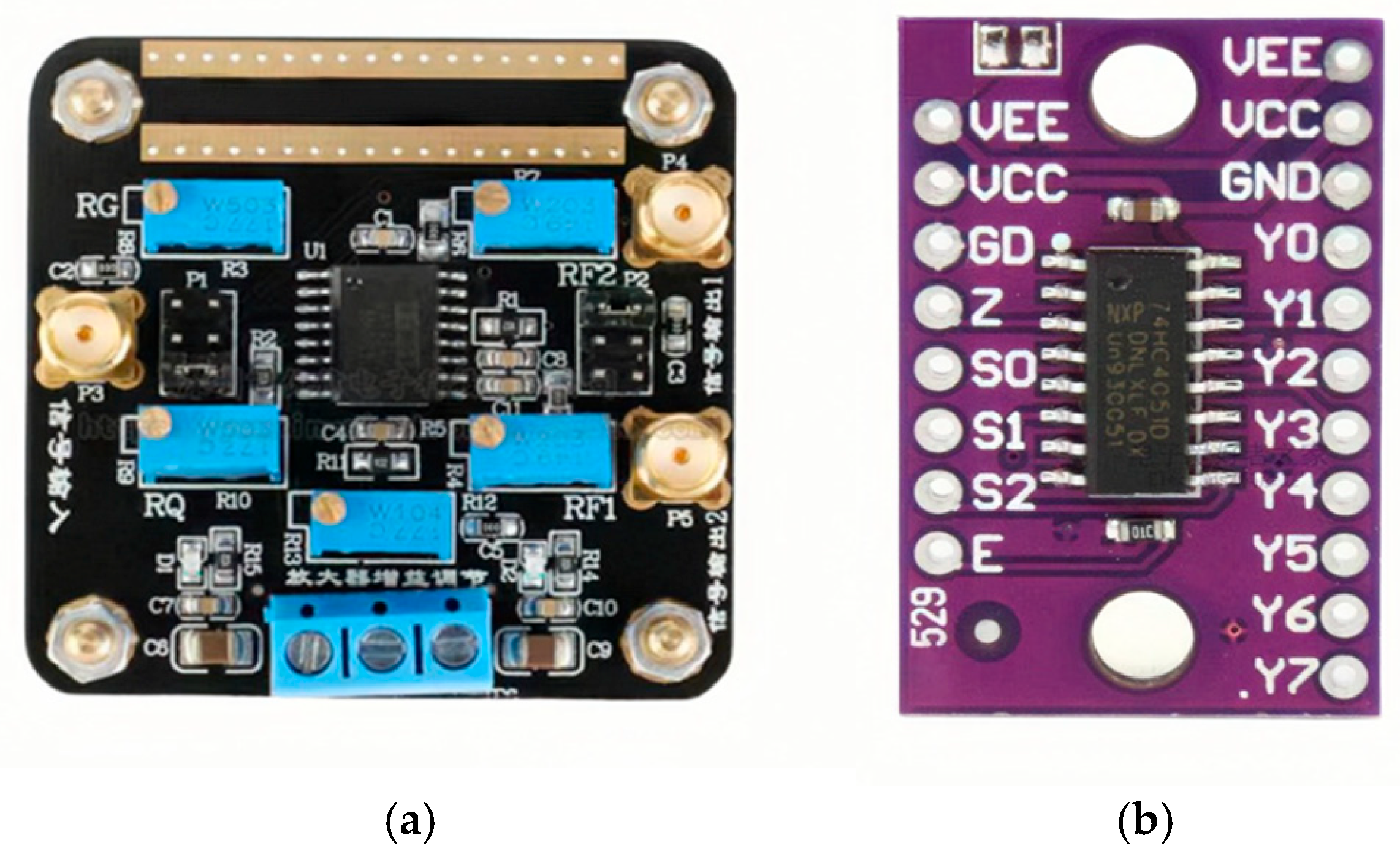
5.3.2. Signal Processing Module

In magnetic flux leakage (MFL) detection for oil and gas pipelines, the detector collects low-frequency MFL signals. When the pipeline surface is defect-free, the signal curve is flat with low amplitude; at a defect or weld, the signal changes abruptly, with significantly increased amplitude. On-site data acquisition is prone to interference, with MFL signals often mixed with high-frequency noise, including system, vibration, and pipeline material noise. Thus, a filtering circuit is needed to suppress high-frequency noise. Hall sensor MFL signals are weak and prone to environmental and circuit interference, reducing resolution and reliability, requiring amplification of the filtered signal via an amplification circuit.

This study uses the UAF42 active filter to filter and amplify Hall sensor signals. The UAF42, with multiple operational amplifiers, supports high-pass, low-pass, or band-pass filtering via simple peripheral circuits and amplifies weak signals by adjusting gain and frequency response, ensuring effective MFL signal processing. Given the noise characteristics of MFL signals, the UAF42 is configured as a low-pass filter, with cutoff frequency adjusted via external resistors and capacitors to pass MFL signals while suppressing high-frequency noise. Gain is set via feedback resistors to match the development board’s input range, preventing data loss or distortion from overly weak or strong signals. As a multi-channel signal acquisition system, a single filter cannot process multiple signals simultaneously; thus, the 74HC4051 multiplexer switch processes signals from multiple Hall sensors sequentially through the UAF42 filter by switching channels. Thus, this study selects the 74HC4051 multiplexer switch and UAF42 active filter as the signal processing module for the MFL detection system, as shown in Figure 30.

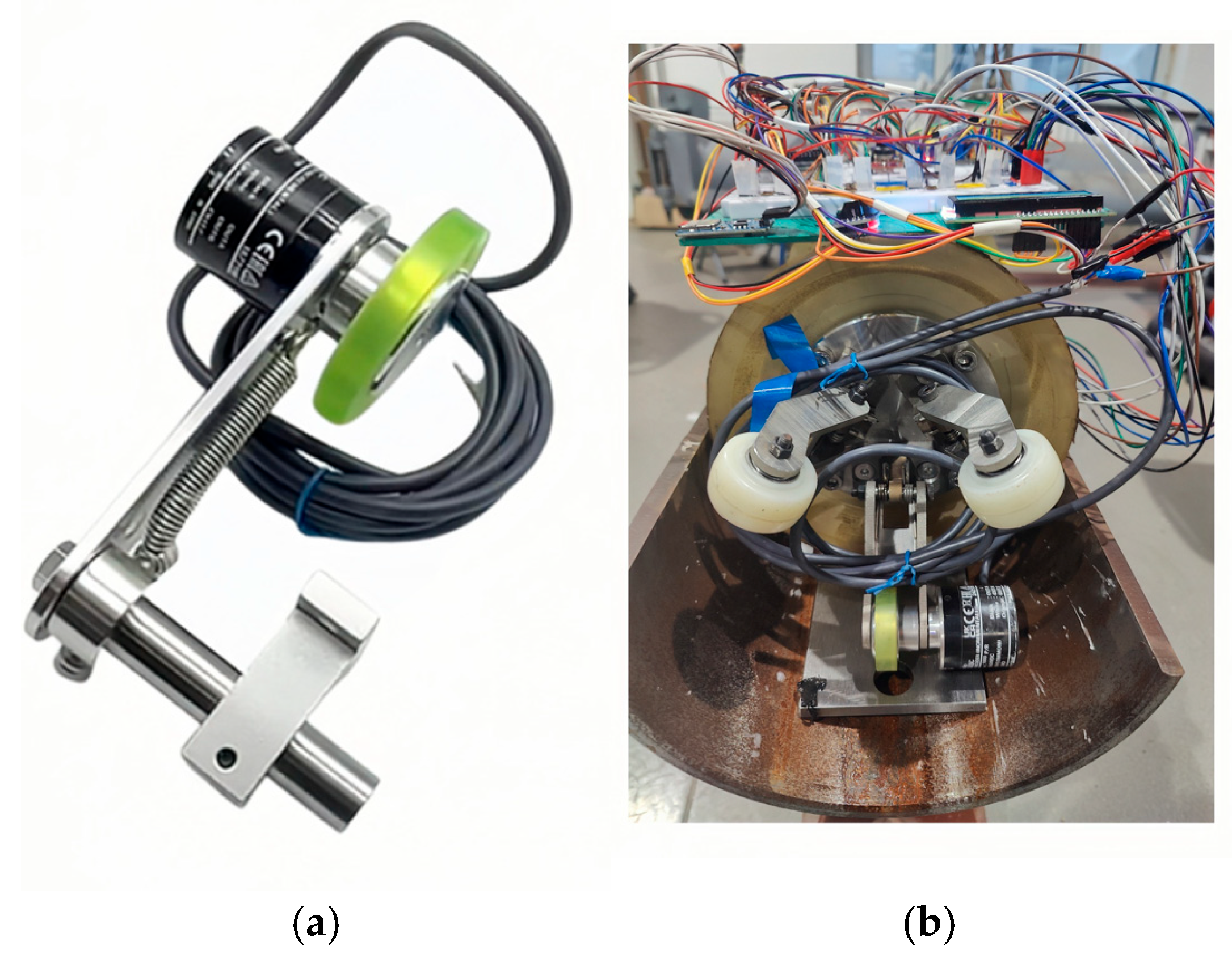
5.3.3. Positioning Information Acquisition Module

To track the travel distance of the magnetic flux leakage (MFL) detector during pipeline inspection and locate defect positions, the design incorporates an odometry wheel positioning module. The odometry wheel comprises a wheel and a rotary encoder. This study selects the Omron E6B2-CWZ6C incremental rotary encoder with a 40 mm diameter support wheel to form the MFL detector’s positioning module, as shown in Figure 31. The E6B2-CWZ6C operates on the photoelectric principle, comprising a rotating shaft, optical code disk, light source, photoelectric sensor, and signal processing circuit. The encoder’s rotating shaft drives the optical code disk, with evenly spaced transparent holes, while a light source on one side and a photosensitive sensor on the other receive light signals. As the optical code disk rotates, its transparent holes produce alternating light signals, converted by the photosensitive sensor into periodic electrical pulses. The E6B2-CWZ6C uses two offset photosensitive sensors to produce orthogonal phase A and B pulse signals with a fixed phase difference, enabling precise determination of rotation direction, angle, and displacement. The optical code disk also features a reference marker slot, producing a Z-phase pulse once per rotation to indicate a complete shaft revolution.

During pipeline inspection, as the magnetic flux leakage (MFL) detector travels, the odometry wheel rotates oppositely, driving the E6B2-CWZ6C encoder to rotate synchronously with the wheel axle, producing pulse signals. The Arduino MEGA 2560 control system collects encoder pulse signals in real-time via an interrupt mechanism, calculating travel distance by counting pulses. The encoder has a resolution of 1000 pulses per revolution (PPR), outputting 1000 pulses per rotation. With a 40 mm wheel diameter and a circumference of approximately 125.7 mm, 1000 pulses correspond to a 125.7 mm travel distance. To ensure measurement accuracy, the encoder output and distance calculation formula require calibration based on the relationship between actual travel distance and pulse count.

The E6B2-CWZ6C encoder operates on a 5 V DC power supply with a simple, reliable wiring design. The encoder’s power pin connects to the Arduino MEGA 2560’s 5 V pin, and its ground line connects to the GND pin. The encoder employs an NPN open-collector output for A, B, and Z phase signals, each requiring a pull-up resistor to the 5 V power supply for a 5 V high-level output, connected to the control system’s digital input pins. This design ensures voltage compatibility and signal stability, enabling precise measurement of rotation direction and travel distance.

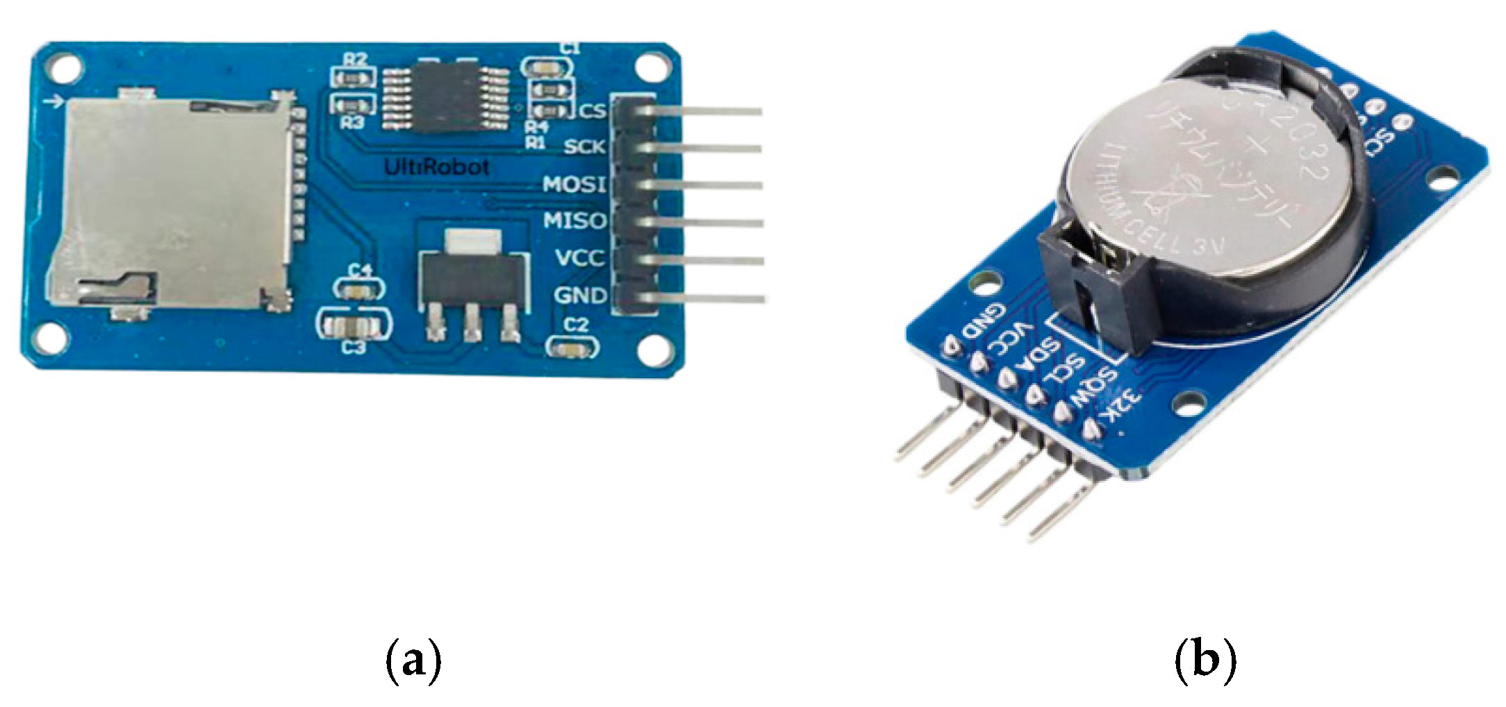
5.3.4. Data Storage Module

The data storage module comprises a Micro SD card module and a DS3231 real-time clock module, as shown in Figure 32. The Micro SD card, a widely used storage medium, provides high storage capacity, fast data transfer rates, and robust stability, supporting SPI and SDIO interfaces. As the control module lacks SDIO support, the SPI interface is used for data transfer with the Arduino development board, and the FAT32 file system ensures stable operation and data compatibility.

The system initializes the Micro SD card using the SD.begin(chipSelect) function before use. Upon successful initialization, the serial monitor displays a prompt indicating the SD card’s data-writing state; if initialization fails, an error message is output via the serial port, halting operation. To include precise timestamps for data organization and analysis, the system incorporates a DS3231 real-time clock module. During data acquisition, the system reads the current time, storing timestamps alongside sensor data on the SD card. Files are opened using the SD.open function and data is written using the File.print and File.println functions in TXT format, including MFL field strength values and corresponding timestamps. The stored data is imported into computational software for analysis, generating MFL signal curves to assess pipeline surface defects.

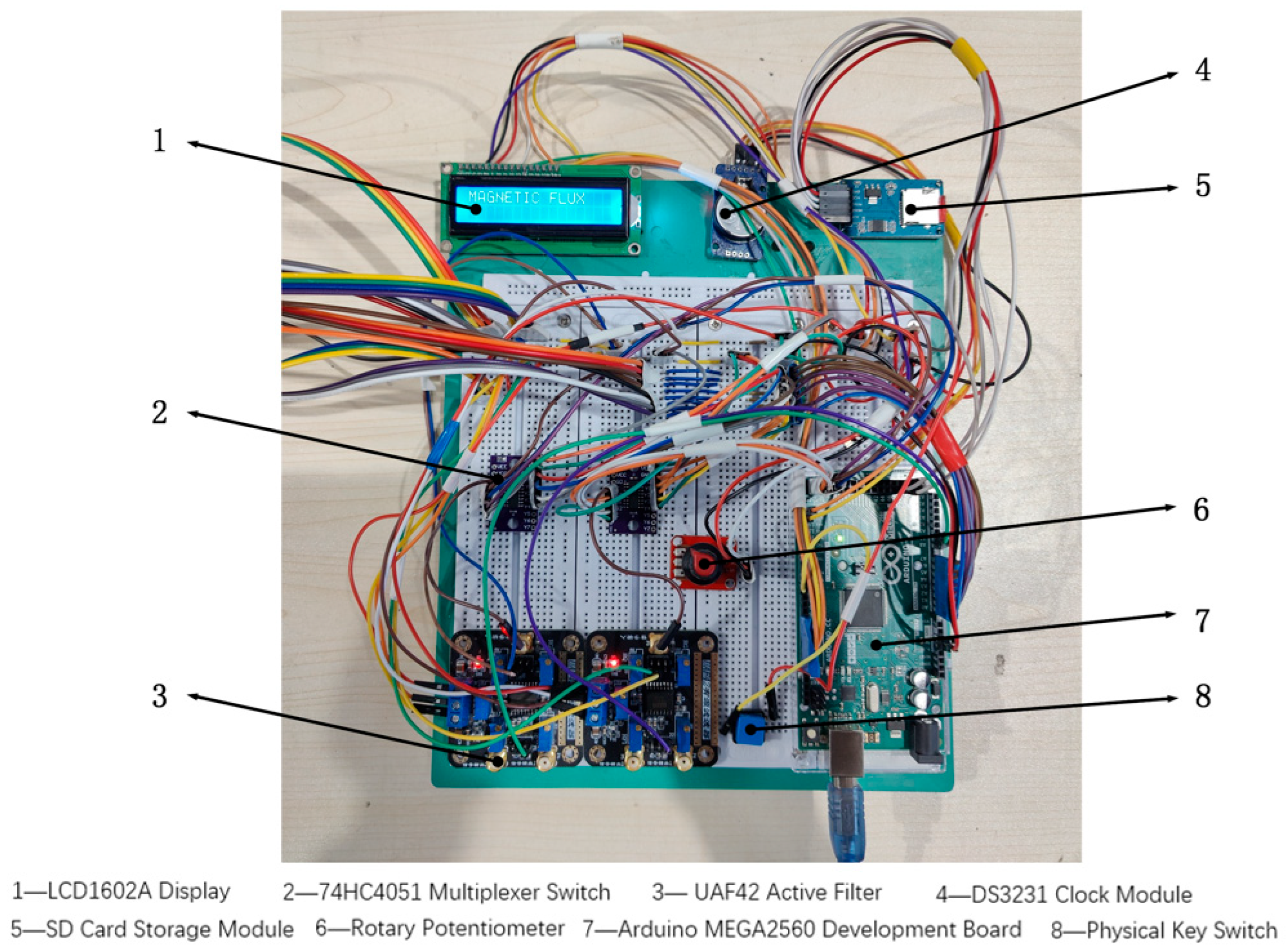
5.3.5. Control System Circuit Design

The magnetic flux leakage (MFL) detection system is assembled using a breadboard and DuPont wires, as shown in Figure 33. This multi-channel acquisition system collects axial and radial MFL components, incorporating two signal processing modules. The 74HC4051 multiplexer switch, controlled by Arduino code, selects signals from multiple Hall sensors for filtering and amplification by the UAF42 filter. Pulse signals from the E6B2-CWZ6C rotary encoder are input to the Arduino MEGA 2560 via digital interfaces. The Micro SD card module connects to the Arduino MEGA 2560 via an SPI interface, while the DS3231 clock module provides precise timestamps via an I2C interface. As the system is PC-powered and lacks independent start–stop control, a push-button switch and LCD1602A display are added, connected to the Arduino’s digital input ports. During signal acquisition, the LCD displays “RECORDING”; when stopped, it displays “MAGNETIC FLUX.” To sample 24 Hall sensors within 5 ms, the system is optimized via hardware–software synergy, using non-blocking programming and timer interrupts for independent data collection. Data is temporarily stored in memory and written to the Micro SD card in batches after processing to minimize storage latency.

6. Experimental Validation

To validate the performance of the magnetic flux leakage (MFL) pig in subsea pipeline defect detection, this study develops an experimental platform to evaluate the effects of varying axial length, radial depth, and sensor lift-off value of rectangular defects on MFL signal distribution patterns, confirm the reliability of prior simulations, and assess the pig’s practical utility.

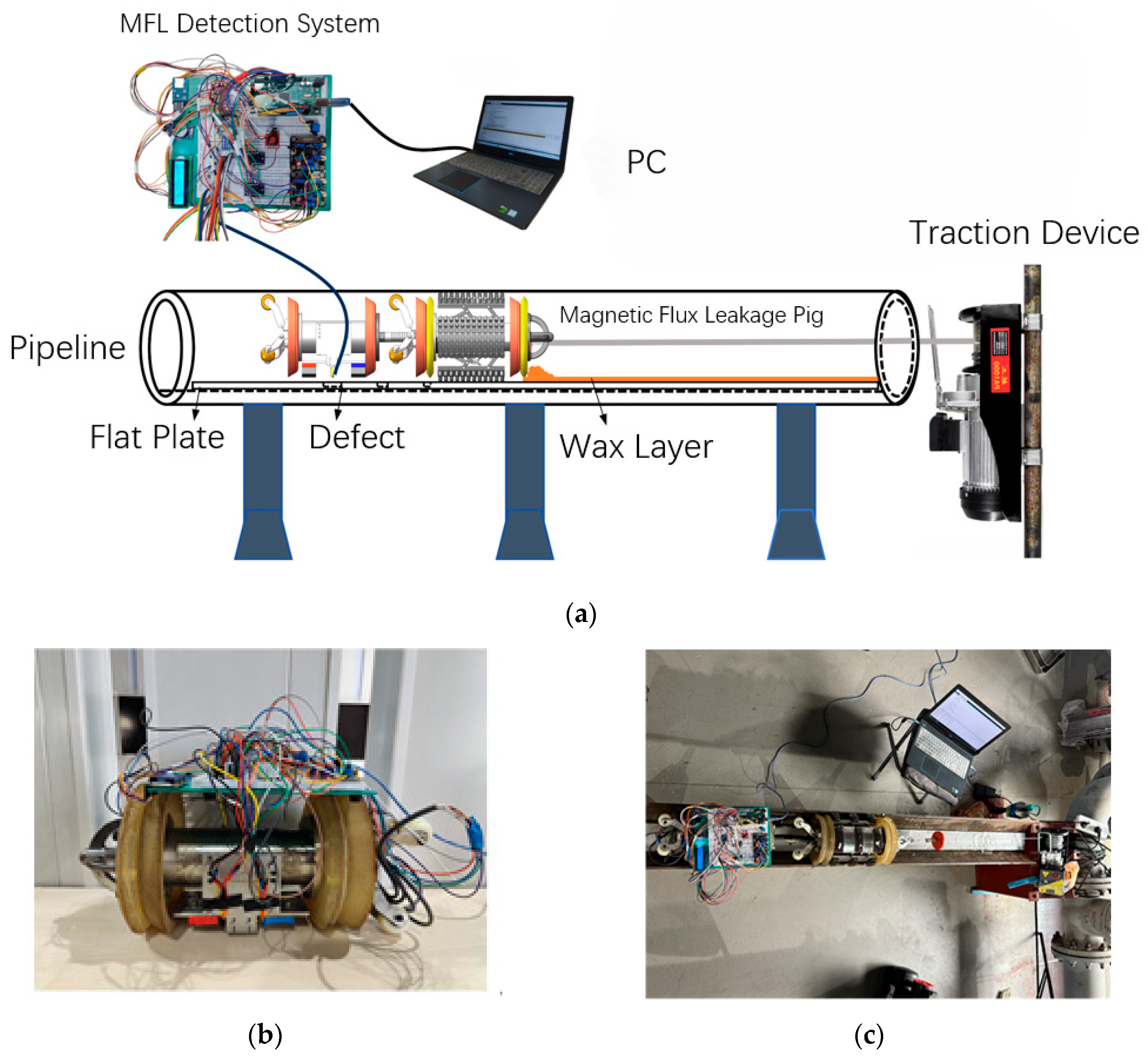
6.1. Simulation Setup

The experimental platform includes the magnetic flux leakage (MFL) pig, a flat plate with artificial defects, the MFL detection system, a traction device, a semi-open pipeline, and a magnetization device, designed to simulate wax deposition and inner wall defects in subsea pipelines. The MFL pig is equipped with a magnetization device and magnetic sensors for MFL detection. The test plate, made of 20# steel with a 15 mm wall thickness, features rectangular defects with axial lengths of 1–10 mm and radial depths of 5–10 mm. The MFL detection system, based on the previously described framework, includes a magnetization module, high-sensitivity magnetic sensors, a signal conditioning circuit, an analog-to-digital conversion module, and a PC-based data processing unit. The traction device moves the pig along the plate at a constant speed of 1–2 m/s; the semi-open pipeline enables inspection process observation and secures the test plate; and the magnetization device uses Nd₂Fe₁₄B permanent magnets, forming a closed magnetic circuit via a yoke and steel brushes for full magnetization. During the experiment, the test plate is placed on the semi-open pipeline’s inner wall, and the pig, driven by the traction device at 1–2 m/s, continuously collects axial (B_z) and radial (B_r) MFL signal components, which are converted via Arduino’s analog-to-digital conversion, transmitted to a PC, and analyzed using computational software for signal waveform characteristics, including peak values and waveform width. The experimental platform and MFL pig prototype are shown in Figure 34.

6.2. Defect Sample Preparation

To validate the accuracy of magnetic flux leakage (MFL) detection simulation results, this study designs two test plates, each with rectangular defects of varying axial lengths and radial depths, to evaluate the effects of defect geometry on MFL signals. Both plates, with a 10 mm thickness, include the following: Plate A, with five uniformly distributed rectangular defects of fixed axial length and radial depths of 1, 3, 5, 7, and 9 mm; and Plate B, with five uniformly distributed rectangular defects of fixed radial depth and axial lengths of 4, 6, 8, 10, and 12 mm. The surface defects’ distribution and dimensions are shown in Figure 35.

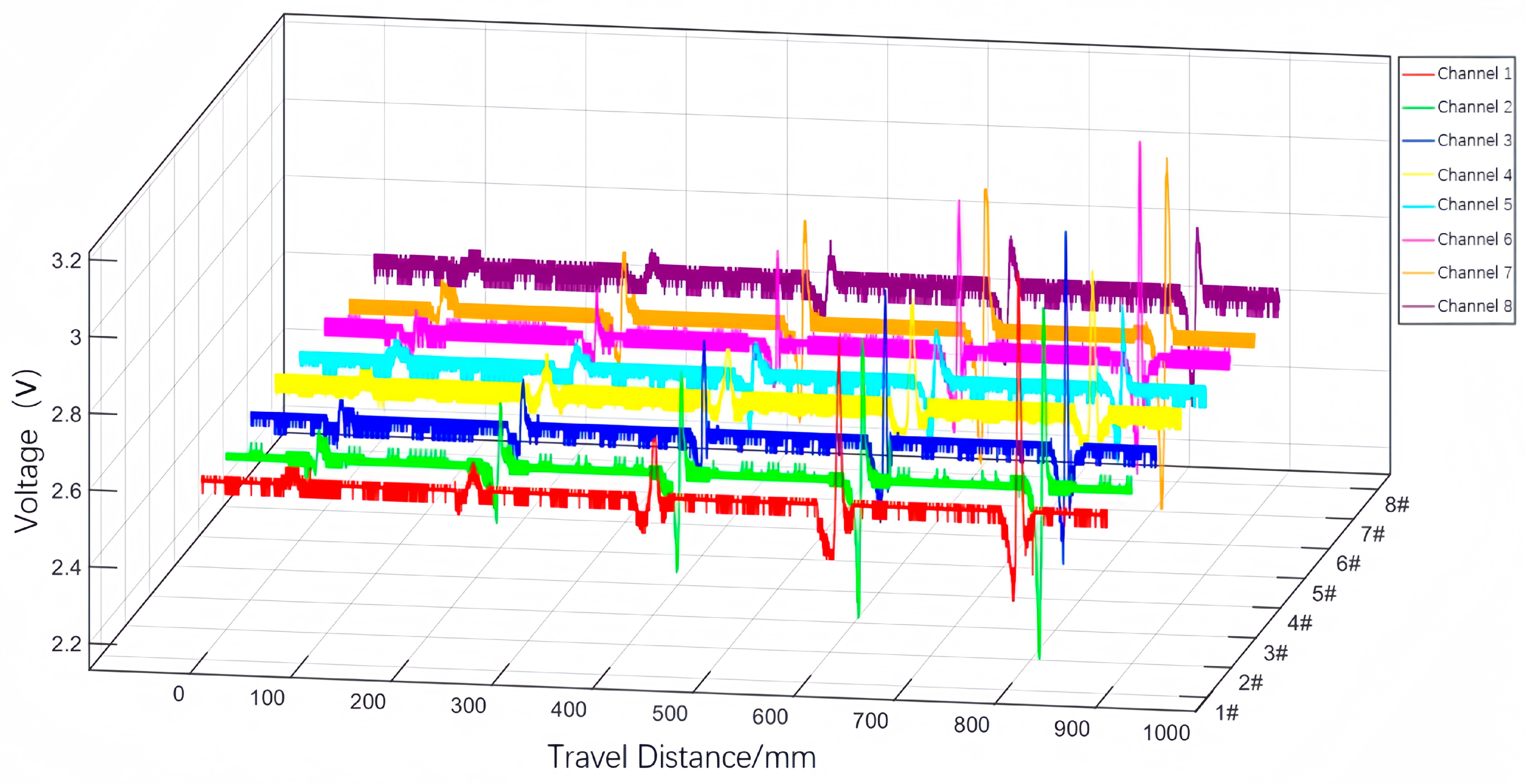
6.3. Experimental Results and Analysis

The detection device, equipped with eight Hall sensors soldered onto a PCB and fixed to the magnetization device for enhanced probe stability, has its layout shown in Figure 36. The orientation of the Hall sensors affects the measurement of axial and radial MFL field components, with four left-side sensors collecting the axial component (channels 1–4) and four right-side sensors collecting the radial component (channels 5–8). Driven by the traction device, the multifunctional MFL pig’s wax removal section clears wax from test plate surfaces with varying defects, while the detection section evaluates the effects of defect radial depth, axial length, and sensor lift-off value on MFL signal distribution patterns.

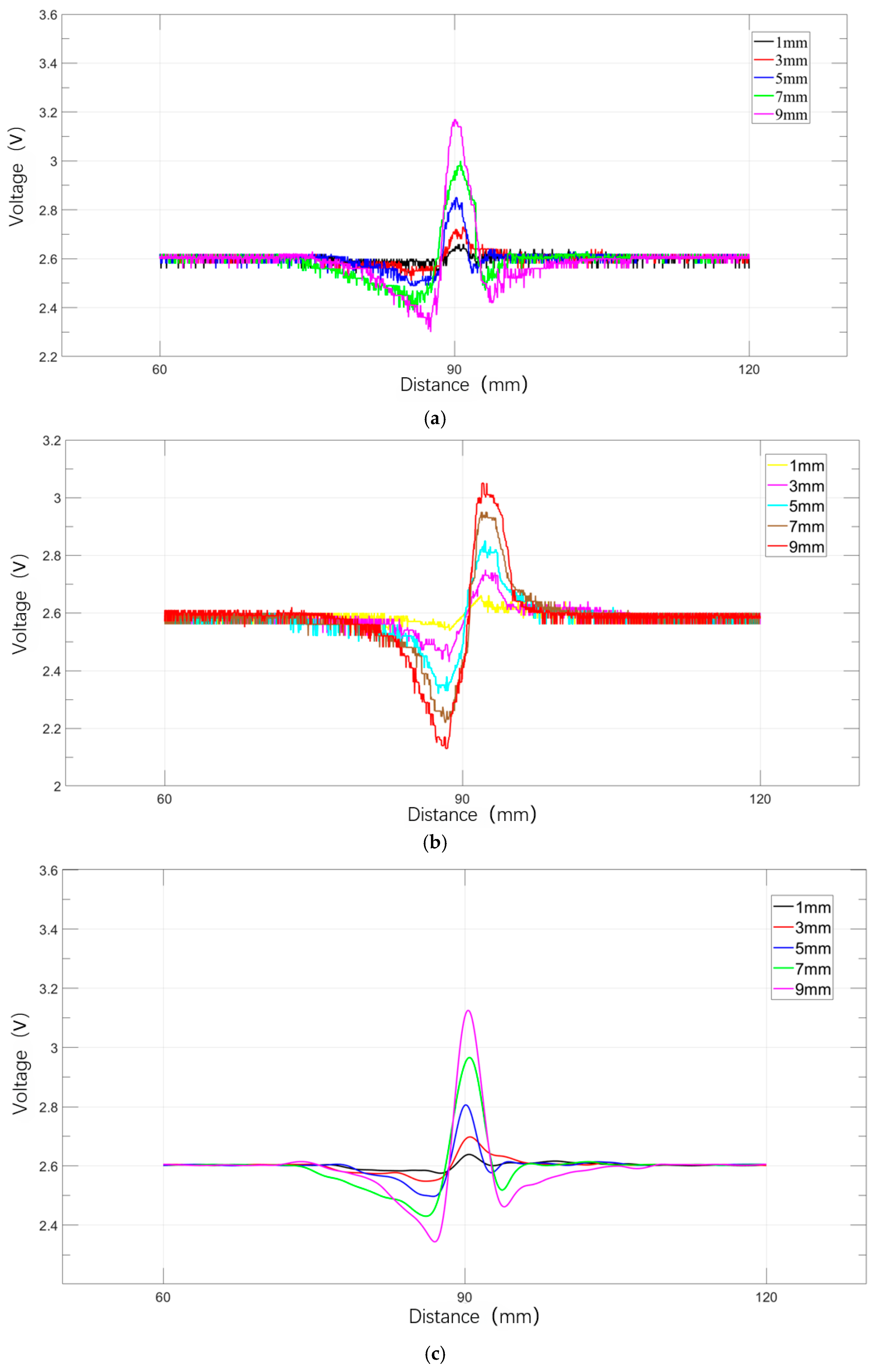
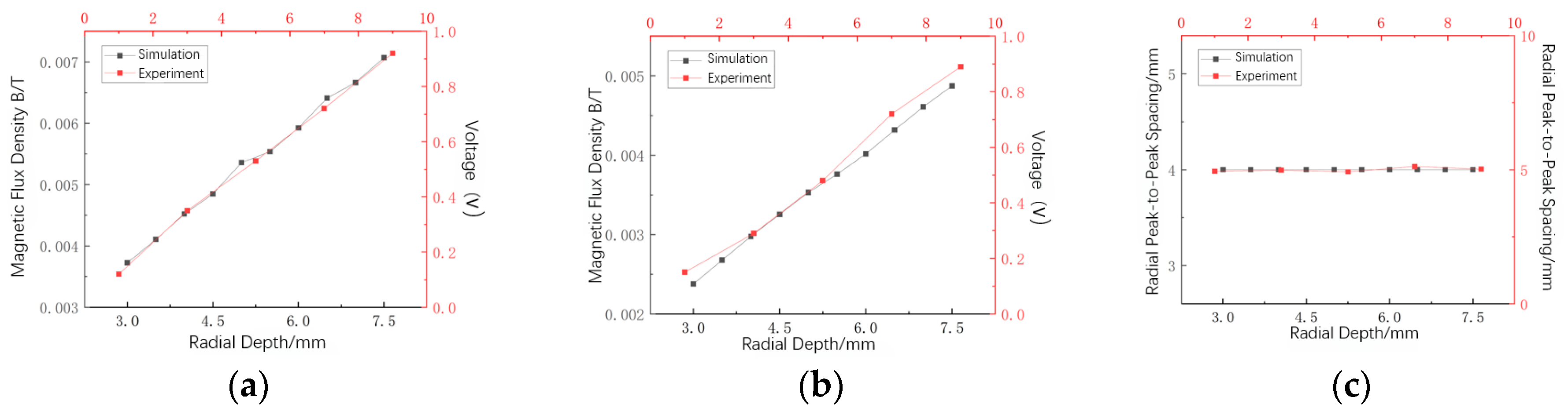
6.3.1. Effect of Rectangular Defect Radial Depth on Magnetic Leakage Signals

Figure 37 shows the waveform patterns of eight MFL signal channels collected by the MFL detection system, varying with defect depths of 1, 3, 5, 7, and 9 mm. Analysis reveals that MFL signal voltage values from multiple Hall sensors fluctuate around 2.6 V, with axial and radial component waveform changes at defects closely matching simulation results. Further analysis shows that for a given defect, signal voltage values vary across channels, with channels 2 and 3 (axial) and 6 and 7 (radial) typically showing higher peak values than others. This phenomenon is attributed to sensor positioning: sensors directly above the defect center yield maximum voltage amplitude, while those in channels 1, 4, 5, and 8, positioned above defect edges, show lower signal strength. For detailed analysis, waveforms from channels 2 and 6 are extracted and smoothed, as shown in Figure 38. The results indicate that increasing rectangular defect depth raises axial and radial component signal peak values, aligning with simulation-derived patterns.

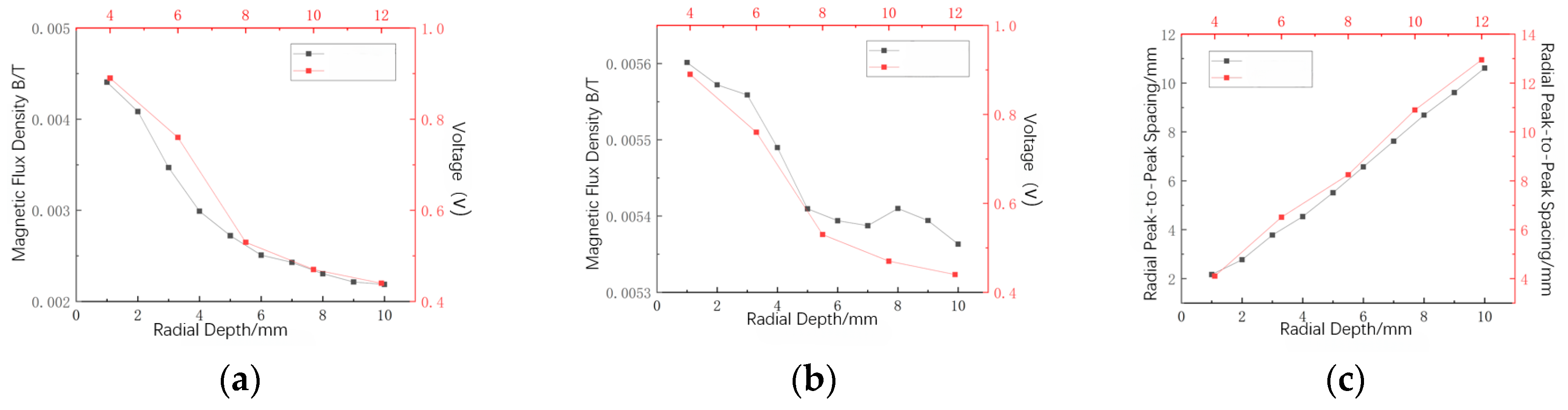
6.3.2. Effect of Axial Length of Rectangular Defects on Magnetic Leakage Signals

As the magnetic flux leakage (MFL) pig moves uniformly past rectangular defects with axial lengths of 4, 6, 8, 10, and 12 mm, the axial and radial MFL signal components collected by each Hall sensor are shown in Figure 39: (a) axial component voltage signal; (b) radial component voltage signal; (c) fitted axial voltage signal; (d) fitted radial voltage signal. To improve detection accuracy, this study extracts signal curves from channels 2 and 6 to evaluate the effect of varying defect longitudinal length on MFL signals. Figure 40 shows that as defect longitudinal length increases, the axial component voltage signal waveform shifts from a single-peak to a double-peak structure, the waveform width of both axial and radial components increases, and peak values decrease, aligning with simulation results.

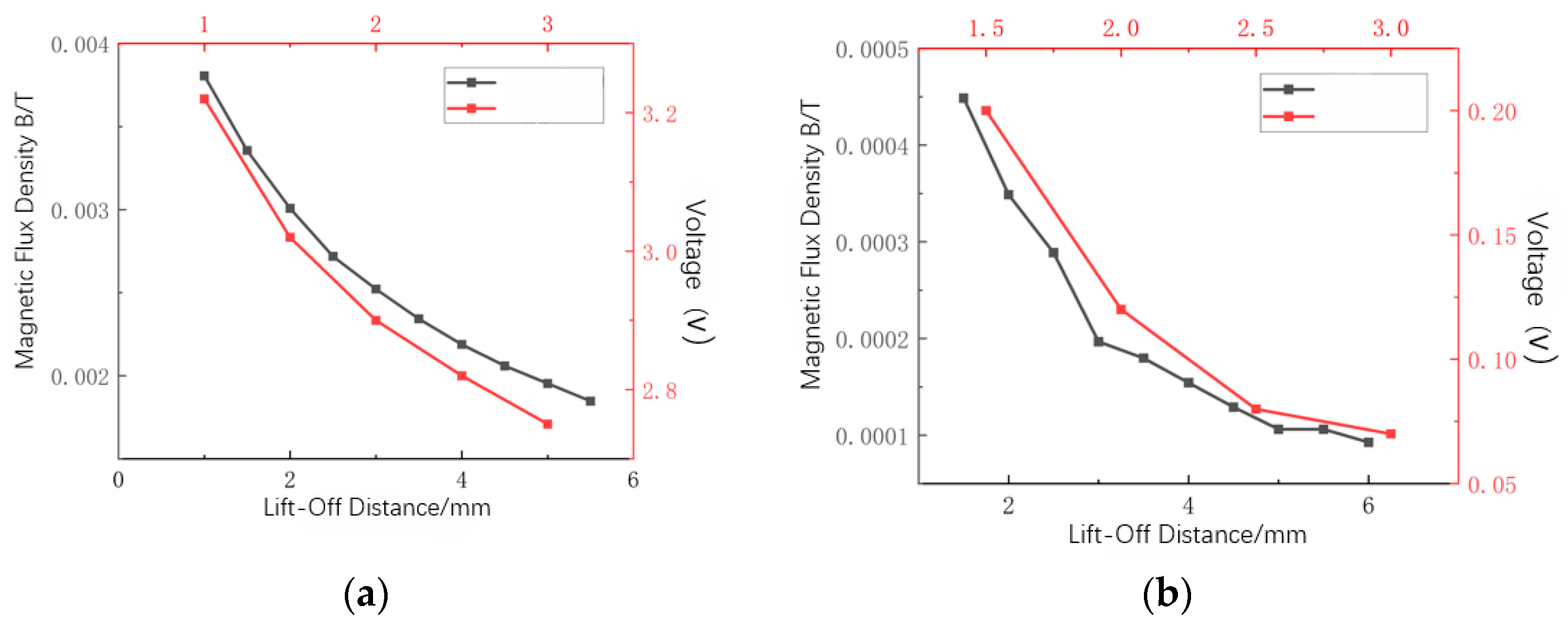
6.3.3. Effect of Rectangular Defect Lift-Off Value Variations on Magnetic Leakage Signals

By adjusting the mounting hole position of the detection device’s magnetization module, the lift-off value between the Hall sensors and the defect surface of the iron plate is precisely controlled. When the detector inspects the same defect with lift-off values sequentially adjusted to 1 mm, 1.5 mm, 2 mm, 2.5 mm, and 3 mm, the variations in the signal curves of the axial and radial components of the magnetic leakage field are shown in Figure 41. After smoothing processing, analysis indicates that the lift-off value significantly affects signal strength: higher lift-off values result in lower magnetic leakage field signal strength, while the effective width of the axial and radial component waveforms remains essentially constant. This pattern is highly consistent with simulation analysis results.

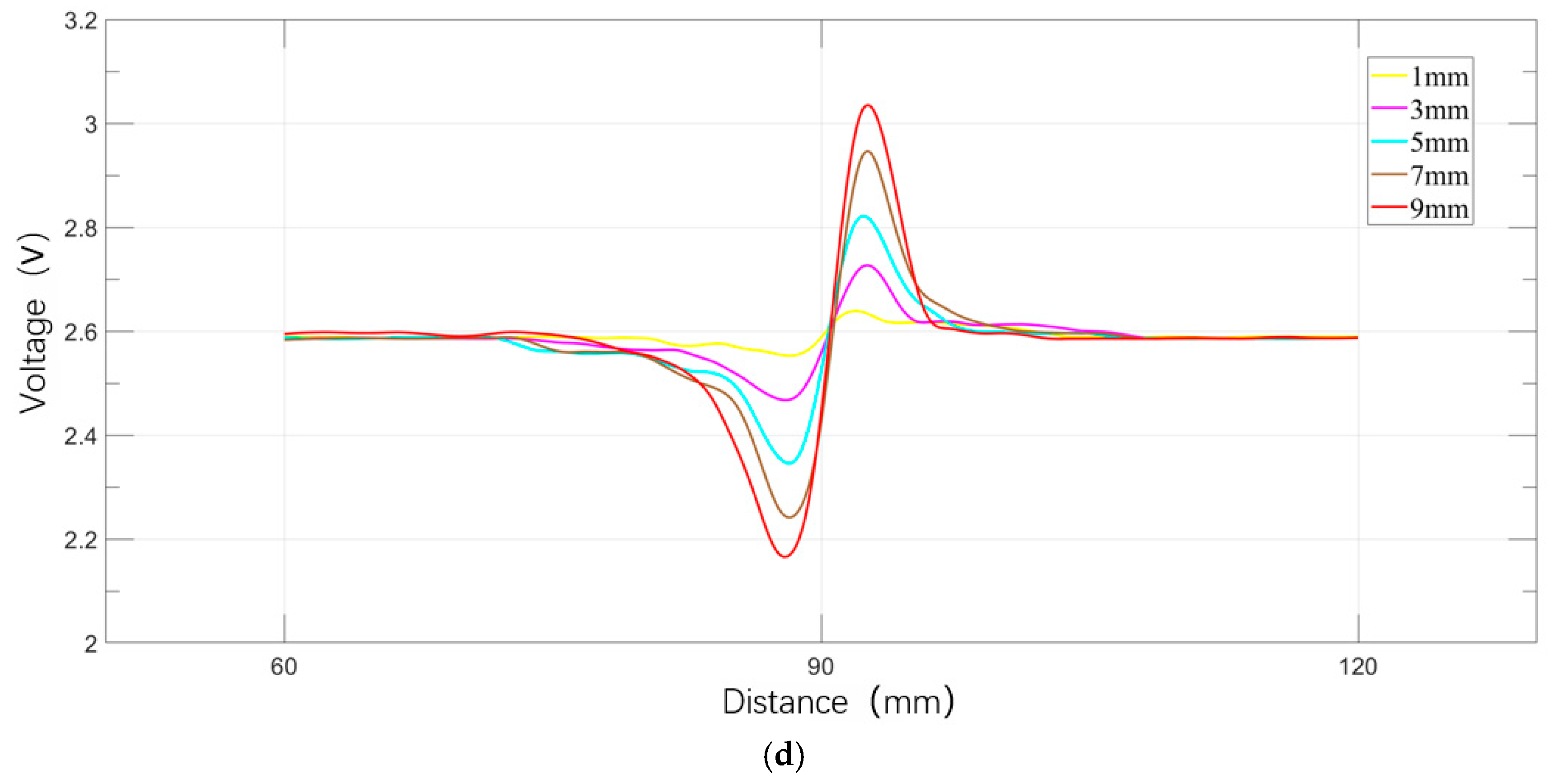
6.4. Comparative Validation of Experimental and Simulation Results

To validate the accuracy of experimental conclusions and the effectiveness of the magnetic flux leakage (MFL) detection system, this study analyzes experimentally collected MFL signal characteristics using prior simulation methods, evaluating the effects of sensor lift-off value, defect longitudinal length, and radial depth on axial peak-to-valley value, radial peak-to-peak value, and radial peak-to-peak spacing, and comparing these with simulation results to assess differences. Figure 42 compares experimental and simulation results for the effects of defect radial depth on axial peak-to-valley value, radial peak-to-peak value, and radial peak-to-peak spacing. Analysis reveals that trends in experimentally measured axial peak-to-valley value, radial peak-to-peak value, and radial peak-to-peak spacing closely align with simulation results. As radial depth increases, axial peak-to-valley and radial peak-to-peak values show near-linear growth, while radial peak-to-peak spacing remains constant, aligning with MFL signal curve characteristics at defect locations. Experimental and simulation results confirm the feasibility of accurately inverting pipeline surface defect depth using axial peak-to-valley and radial peak-to-peak values.

Figure 43 compares experimental and simulation results for the effects of defect longitudinal length on axial peak-to-valley value, radial peak-to-peak value, and radial peak-to-peak spacing. Experimental results indicate that as defect longitudinal length increases, axial peak-to-valley and radial peak-to-peak values of MFL signals decrease, while radial peak-to-peak spacing increases, aligning with simulation trends. Axial peak-to-valley value and radial peak-to-peak spacing variations closely match simulations, while radial peak-to-peak value fluctuations are slightly smaller than simulated values. As both experimental and simulation results show linear changes in radial peak-to-peak spacing, it serves as a reliable parameter for inverting defect longitudinal length.

Simulation analysis reveals that lift-off value variations mainly affect MFL signal peak strength, with higher lift-off values reducing signal strength. Figure 44 shows the experimental trend of axial component peak value with varying lift-off values, closely aligning with simulation results, both exhibiting consistent peak variation patterns and magnitude changes with lift-off adjustments. Signal peak amplitude varies significantly across different lift-off value ranges. Thus, in pipeline inspections, the lift-off value range should be optimized based on field conditions to minimize signal peak variations and reduce lift-off fluctuation interference in signal acquisition.

This study evaluates the effects of sensor lift-off value, defect longitudinal length, and radial depth on MFL signal parameters (axial peak-to-valley value, radial peak-to-peak value, and radial peak-to-peak spacing). Results show that increasing radial depth causes near-linear growth in peak values, increasing axial length reduces peak values while increasing spacing, and higher lift-off values significantly decrease signal strength while waveform width remains constant. Experimental and simulation results closely align, confirming the feasibility of inverting defect dimensions using these parameters.

7. Conclusions and Outlook

Using 3D finite element simulation and experimental validation, this study evaluates the performance of the magnetic flux leakage (MFL) pig in subsea pipeline defect detection, analyzing the effects of defect geometry, excitation intensity, sensor lift-off, and operating speed on MFL signals, and achieves precise defect dimension quantification via characteristic parameter inversion, providing theoretical and practical guidance for pipeline integrity management.

Simulation analysis reveals that MFL signals are highly sensitive to defect geometry. Rectangular defects yield the strongest MFL signal strength and widest waveform width, with the axial component (B_z) showing a double-peak–double-valley structure and the radial component (B_r) exhibiting a single-peak–single-valley structure. At a defect longitudinal length of 4 mm, the axial component signal shifts from a single peak to a double peak, with waveform width increasing with length. Increasing radial depth causes linear increases in axial peak-to-valley and radial peak-to-peak values, while radial peak-to-peak spacing remains constant. Asymmetric defects, such as triangular defects, cause signal peak shifts without reducing signal strength. Excitation intensity peaks in signal increment at 2.4 T, entering saturation beyond 4.0 T. Increasing lift-off from 1 mm to 6 mm reduces signal strength by approximately 60%, with 3–5 mm as the optimal range for balancing vibration interference and detection accuracy. Increasing operating speed to 4 m/s induces signal distortion and strength reduction, requiring enhanced excitation to maintain detection robustness. These results show that defect geometry, excitation intensity, lift-off, and operating speed determine MFL signal distribution characteristics, providing parameters for optimizing pig performance.

Experimental validation confirms the reliability of simulation results. On an experimental platform simulating subsea pipeline conditions, the MFL pig was tested for rectangular defect longitudinal length, radial depth, and lift-off. Experimental signal waveforms closely align with simulations: axial peak-to-valley value increases linearly with radial depth, radial peak-to-peak spacing increases linearly with axial length, and higher lift-off reduces signal strength without affecting waveform width. For example, at a 4 mm axial length, the axial component signal shows a double-peak structure; at a 6 mm lift-off, the signal peak value decreases by approximately 60%, aligning with simulation predictions. Comparison of experimental and simulation results confirms the feasibility of inverting defect dimensions using radial peak-to-valley value and radial peak-to-peak value for axial length, and axial peak-to-valley value for radial depth. These parameters provide a reliable basis for quantitative defect assessment, enhancing detection accuracy.

Simulation and experimental results demonstrate the MFL pig’s high sensitivity and robustness in subsea pipeline defect detection, offering an effective solution for pipeline integrity management in complex marine environments. However, this study has limitations, including limited consideration of pipeline material non-uniformity, subsea current interference, and multi-defect signal interactions. Future research will enhance simulation models with multi-physics coupling to better replicate marine conditions. Real-time signal processing algorithms will be developed to replace offline analysis, enhancing detection efficiency. Optimizing inversion algorithms with machine learning will improve dimension inference accuracy in multi-defect scenarios. Full-scale pipeline experiments are planned to validate the pig’s performance in long-distance, high-pressure environments, supporting industrial application. These efforts will advance MFL detection technology for subsea pipeline maintenance, ensuring reliable energy transportation safety.

References

1. Bejinaru, C.; Burduhos-Nergis, D.; Cimpoesu, N. Immersion behavior of carbon steel, phosphate carbon steel and phosphate and painted carbon steel in saltwater. Materials 2021, 14, 188. [Google Scholar] [CrossRef]
2. Salgar-Chaparro, S.J.; Lepkova, K.; Pojtanabuntoeng, T.; Darwin, A.; Machuca, L.L. Nutrient level determines biofilm characteristics and subsequent impact on microbial corrosion and biocide effectiveness. Appl. Environ. Microbiol. 2020, 86, e02885-19. [Google Scholar] [CrossRef]
3. Vanaei, H.R.; Eslami, A.; Egbewande, A. A review on pipeline corrosion, in-line inspection (ILI), and corrosion growth rate models. Int. J. Press. Vessels Pip. 2017, 149, 43–54. [Google Scholar] [CrossRef]
4. Chen, J.; Jia, G.; Fu, K.; Zhang, H. Integrity Assessment of Moda Crude Oil Pipeline Based on Multi In-Line Inspection Datasets. In Proceedings of the 12th International Conference on Quality, Reliability, Risk, Maintenance, and Safety Engineering (QR2MSE 2022), Emeishan, China, 27 July 2022; pp. 1482–1486. [Google Scholar]
5. Verma, A.; Kaiwart, A.; Dubey, N.D. A review on various types of in-pipe inspection robot. Mater. Today Proc. 2022, 50, 1425–1434. [Google Scholar] [CrossRef]
6. Peng, X.; Anyaoha, U.; Liu, Z.; Tsukada, K. Analysis of magnetic-flux leakage (MFL) data for pipeline corrosion assessment. IEEE Trans. Magn. 2020, 56, 6200315. [Google Scholar] [CrossRef]
7. Liu, B.; Luo, N.; Feng, G. Quantitative study on MFL signal of pipeline composite defect based on improved magnetic charge model. Sensors 2021, 21, 3412. [Google Scholar] [CrossRef] [PubMed]
8. Yee, K.J. Numerical solution of initial boundary value problems involving Maxwell’s equations in isotropic media. IEEE Trans. Antennas Propag. 1966, 14, 302–307. [Google Scholar]
9. Zatsepin, N.J. Calculation of the magnetostatic field of surface defects. I Field Topogr. Defect Models Defectoscopy 1966, 5, 50–59. [Google Scholar]
10. Shcherbinin, V.J. Calculation of the magnetostatic field of surface defects. II Exp. Verif. Princ. Theor. Relatsh. Defectoscopy 1966, 5, 59–65. [Google Scholar]
11. Hwang, J.; Lord, W. Finite element modeling of magnetic field defect interactions. J. Test. Eval. 1975, 3, 21–25. [Google Scholar] [CrossRef]
12. Coramik, M.; Citak, H.; Ege, Y.; Bicakci, S.; Gunes, H. Determining the effect of velocity on sensor selection and position in non-destructive testing with magnetic flux leakage method: A pipe inspection gauge design study with ANSYS Maxwell. IEEE Trans. Instrum. Meas. 2023, 72, 1–12. [Google Scholar] [CrossRef]
13. Keshwani, R. Analysis of magnetic flux leakage signals of instrumented pipeline inspection gauge using finite element method. IETE J. Res. 2009, 55, 73–82. [Google Scholar] [CrossRef]
14. Piotrowski, C.M. Analysis of the magnetic flux leakage signal detected by a pipeline inspection gauge with the help of the continuous wavelet transform. J. Electr. Eng. 2015, 66, 182–185. [Google Scholar]
15. Adegboye, M.A.; Fung, W.-K.; Karnik, A. Recent Advances in Pipeline Monitoring and Oil Leakage Detection Technologies: Principles and Approaches. Sensors 2019, 19, 2548. [Google Scholar] [CrossRef]
16. Meniconi, S.; Brunone, B.; Tirello, L.; Rubin, A.; Cifrodelli, M.; Capponi, C. Transient tests for checking the Trieste subsea pipeline: Towards the field tests. J. Mar. Sci. Eng. 2024, 12, 374. [Google Scholar] [CrossRef]
17. Meniconi, S.; Brunone, B.; Tirello, L.; Rubin, A.; Cifrodelli, M.; Capponi, C. Transient tests for checking the Trieste subsea pipeline: Diving into fault detection. J. Mar. Sci. Eng. 2024, 12, 391. [Google Scholar] [CrossRef]
18. Mukherjee, D.; Saha, S.; Mukhopadhyay, S. An adaptive channel equalization algorithm for MFL signal. NDT E Int. 2012, 45, 111–119. [Google Scholar] [CrossRef]
19. Kim, Y.; Shin, J.; Lim, J. Design of spider-type non-destructive testing device using magnetic flux leakage. In Proceedings of the 2019 IEEE Student Conference on Electric Machines and Systems, Busan, Republic of Korea, 1–3 November 2019; pp. 1–4. [Google Scholar]
20. Xin, J.; Li, R.; Chen, J. A crack characterization model for subsea pipeline based on spatial magnetic signals features. Ocean Eng. 2023, 274, 114112. [Google Scholar] [CrossRef]
21. Guo, X.T.; Yang, L.; Song, Y.P. Design and validation of a triaxial high-definition magnetic flux leakage in-pipe inspection robot for oil and gas pipelines. Instrum. Tech. Sens. 2020, 12, 53–57. [Google Scholar]
22. Piao, G.; Guo, J.; Hu, T. Fast reconstruction of 3-D defect profile from MFL signals using key physics-based parameters and SVM. NDT E Int. 2019, 103, 26–38. [Google Scholar] [CrossRef]
23. Wang, W.; Zhang, H.; Li, C.; Du, F.; Chen, J.; Feng, Q.; Cai, M. In-line inspection (ILI) techniques for subsea pipelines: State-of-the-art. J. Mar. Sci. Eng. 2024, 12, 417. [Google Scholar] [CrossRef]
24. Wang, G.; Xia, Q.; Yan, H.; Bei, S.; Zhang, H.; Geng, H.; Zhao, Y. Research on pipeline stress detection method based on double magnetic coupling technology. Sensors 2024, 24, 6463. [Google Scholar] [CrossRef] [PubMed]
25. Kim, J.W.; Park, S. Magnetic flux leakage sensing and artificial neural network pattern recognition-based automated damage detection and quantification for wire rope non-destructive evaluation. Sensors 2018, 18, 109. [Google Scholar] [CrossRef] [PubMed]
26. Xiong, Y.; Liu, S.; Hou, L.; Zhou, T. Magnetic flux leakage defect size estimation method based on physics-informed neural network. Philos. Trans. R. Soc. A 2024, 382, 20220387. [Google Scholar] [CrossRef] [PubMed]
27. Li, Y.; Sun, C. Research on magnetic flux leakage testing of pipelines by finite element simulation combined with artificial neural network. Int. J. Press. Vessels Pip. 2024, 212 Pt A, 105338. [Google Scholar] [CrossRef]
28. Parlak, B.O.; Yavasoglu, H.A. A Comprehensive Analysis of In-Line Inspection Tools and Technologies for Steel Oil and Gas Pipelines. Sustainability 2023, 15, 2783. [Google Scholar] [CrossRef]
29. Zhang, B.; Tang, J.; Zhang, S.; Kang, Y.; Zhang, Y.; Sun, Y. Study on the impact of pole spacing on magnetic flux leakage detection under oversaturated magnetization. Sensors 2024, 24, 5195. [Google Scholar] [CrossRef]
30. Aulin, A.; Shahzad, K.; MacKenzie, R.; Bott, S. Comparison of Non-Destructive Examination Techniques for Crack Inspection; American Society of Mechanical Engineers: Lawrence, KS, USA, 2021. [Google Scholar]
Figure 1. Magnetic flux leakage inspection tools from Rosen Group.
Jmse 13 01462 g001
Figure 2. Schematic diagram of the MFL inspection principle: (a) pipeline without defects; (b) pipeline with defects; (c) MFL field schematic; (d) schematic diagram of the magnetic circuit of the MFL device.
Jmse 13 01462 g002
Figure 3. Finite element simulation model.
Jmse 13 01462 g003
Figure 4. Finite element simulation model: (a) gap air domain; (b) air enclosure domain.
Jmse 13 01462 g004
Figure 5. B-H curves of each component: (a) permanent magnet; (b) yoke; (c) steel brush; (d) pipeline.
Jmse 13 01462 g005
Figure 6. Meshing results: (a) air domain meshing results; (b) simulation model meshing results.
Jmse 13 01462 g006
Figure 7. Contour map of volume magnetic flux density distribution.
Jmse 13 01462 g007
Figure 8. Two-dimensional contour map of magnetic flux density distribution at the defect location: (a) axial component; (b) radial component.
Jmse 13 01462 g008
Figure 9. Three-dimensional contour map of magnetic flux density distribution at the defect location: (a) Axial Component; (b) Radial Component.
Jmse 13 01462 g009
Figure 10. Schematic diagrams of different types of defects.
Jmse 13 01462 g010
Figure 11. Axial and radial MFL field distribution contour maps for various defect types: (a) rectangular defect; (b) symmetric triangular defect; (c) trapezoidal defect; (d) asymmetric triangular defect.
Jmse 13 01462 g011
Figure 12. Effect of defect geometry on the intensity of axial and radial MFL signals: (a) axial component; (b) radial component.
Jmse 13 01462 g012
Figure 13. Effect of defect longitudinal length variation on axial and radial MFL signal intensity: (a) axial component; (b) radial component.
Jmse 13 01462 g013
Figure 14. Variation of the three axial characteristic quantities of the leakage magnetic signal: (a) axial peak-to-valley value; (b) radial peak-to-peak value; (c) radial peak-to-peak spacing.
Jmse 13 01462 g014
Figure 15. Axial and radial MFL signal responses under different defect radial depths: (a) axial component; (b) radial component.
Jmse 13 01462 g015
Figure 16. Variation of the three radial characteristic quantities of the leakage magnetic signal: (a) axial peak-to-valley value; (b) radial peak-to-peak value; (c) radial peak-to-peak spacing.
Jmse 13 01462 g016
Figure 17. Effect of excitation intensity variation on axial and radial MFL signal strength: (a) axial component; (b) radial component.
Jmse 13 01462 g017
Figure 18. Variation of axial and radial MFL signal peak values with excitation intensity: (a) variation in axial magnetic induction intensity peak value; (b) incremental change in axial magnetic induction intensity peak value; (c) variation in radial magnetic induction intensity peak value; (d) incremental change in radial magnetic induction intensity peak value.
Jmse 13 01462 g018
Figure 19. Effect of lift-off changes on the intensity of MFL signals in axial and radial directions: (a) axial component; (b) radial component.
Jmse 13 01462 g019
Figure 20. Effect of lift-off on the axial component peak value of the MFL signal: (a) variation in axial peak value; (b) incremental change in axial peak value.
Jmse 13 01462 g020
Figure 21. Magnetic field distribution under different inspection speeds: (a) 0 m/s; (b) 1 m/s; (c) 2 m/s; (d) 3 m/s; (e) 4 m/s.
Jmse 13 01462 g021
Figure 22. Influence of inspection speed on axial and radial magnetic flux leakage signal intensity: (a) axial component; (b) radial component.
Jmse 13 01462 g022
Figure 23. Block diagram of the MFL detection system.
Jmse 13 01462 g023
Figure 24. Structural model of the magnetizing unit.
Jmse 13 01462 g024
Figure 25. Structural model of the magnetizing unit: R1 (yoke internal reluctance), R2 (air gap between magnets), R5 and R6 (steel brushes), R7 (air gap between steel brushes), R8 and R10 (defect-free pipeline segments), and R9 (pipeline at defect).
Jmse 13 01462 g025
Figure 26. SS495A hall element.
Jmse 13 01462 g026
Figure 27. Structure and arrangement of the detection probes: (a) probe structure illustration; (b) detection probe arrangement.
Jmse 13 01462 g027
Figure 28. Assembly drawing of the magnetization and detection device.
Jmse 13 01462 g028
Figure 29. Arduino MEGA 2560 development board.
Jmse 13 01462 g029
Figure 30. Signal processing module: (a) UAF42 active filter; (b) 74HC4051 multiplexer switch.
Jmse 13 01462 g030
Figure 31. Mileage wheel positioning and data acquisition module: (a) E6B2-CWZ6C encoder; (b) assembled component diagram.
Jmse 13 01462 g031
Figure 32. Data storage module: (a) Micro SD card module; (b) DS3231 real-time clock module.
Jmse 13 01462 g032
Figure 33. Magnetic flux leakage detection control system.
Jmse 13 01462 g033
Figure 34. Actual scene of the prototype and test platform: (a) schematic diagram of the experimental platform; (b) experimental prototype; (c) experimental platform.
Jmse 13 01462 g034
Figure 35. Test Specimens A and B: (a) test plate A with varying defect depths; (b) test plate B with varying defect lengths; (c) flat plate A physical diagram; (d) flat plate B physical diagram.
Jmse 13 01462 g035
Figure 36. Sensor layout and installation: (a) sensor layout; (b) sensor assembly.
Jmse 13 01462 g036
Figure 37. Variation of eight-channel voltage signals at different defect depths.
Jmse 13 01462 g037
Figure 38. Defect Voltage Signals of Channels 2 and 6 at Different Radial Depths: (a) axial component voltage signal; (b) radial component voltage signal; (c) fitted axial voltage signal; (d) fitted radial voltage signal.
Jmse 13 01462 g038aJmse 13 01462 g038b
Figure 39. Variation of eight-channel voltage signals at different defect lengths.
Jmse 13 01462 g039
Figure 40. Defect Voltage Signals of Channels 2 and 6 at Different Axial Lengths: (a) Axial Component Voltage Signal; (b) Radial Component Voltage Signal; (c) Fitted Axial Voltage Signal; (d) Fitted Radial Voltage Signal.
Jmse 13 01462 g040aJmse 13 01462 g040b
Figure 41. Defect Voltage Signals of Channels 2 and 6 at Different Lift-Off Values: (a) axial component voltage signal; (b) radial component voltage signal; (c) fitted axial voltage signal; (d) fitted radial voltage signal.
Jmse 13 01462 g041aJmse 13 01462 g041b
Figure 42. Comparison of simulated and measured characteristic parameters at different defect depths: (a) axial peak-to-valley value; (b) radial peak-to-peak value; (c) radial peak-to-peak spacing.
Jmse 13 01462 g042
Figure 43. Comparison of simulated and measured characteristic parameters at different defect lengths: (a) axial peak-to-valley value; (b) radial peak-to-peak value; (c) radial peak-to-peak spacing.
Jmse 13 01462 g043
Figure 44. Comparison of simulated and measured characteristic parameters at different lift-off values: (a) variation in axial magnetic induction intensity peak value; (b) incremental change in axial magnetic induction intensity peak value.
Jmse 13 01462 g044