Site-Specific Extreme Wave Analysis for Korean Offshore Wind Farm Sites Using Environmental Contour Methods

Abstract

Reliable estimation of extreme waves is essential for offshore wind turbine system design; however, site-specific conditions limit the application of one-size-fits-all statistical methods. We analyzed extreme wave conditions at potential offshore wind farm sites in South Korea using high-resolution hindcast data (1979–2022) based on the Weather Research and Forecasting (WRF) model. While previous studies have typically relied on a limited combination of distribution types and parameter estimation methods, this study systematically applied various Weibull distribution models and parameter estimation techniques to the environmental contour (EC) method. The results show that the optimal statistical approach varied by site according to the tail characteristics of the wave height distribution. The inverse second-order reliability method (I-SORM) provided the highest accuracy in regions with rapidly decaying tails, achieving root mean square error (RMSE) values of 0.21 in Shinan (using the three-parameter Weibull distribution with maximum likelihood estimation, MLE) and 0.34 in Chujado (with the method of moments, MOM). In contrast, the inverse first-order reliability method (I-FORM) yielded superior performance in areas where the tail decays more gradually, such as Yokjido (RMSE = 0.47 with MLE using the exponentiated Weibull distribution) and Ulsan (RMSE = 0.29, with MLE using the exponentiated Weibull distribution). These findings underscore the importance of selecting site-specific combinations of statistical models and estimation techniques based on wave distribution characteristics, thereby improving the accuracy and reliability of extreme design wave predictions. The proposed framework can significantly contribute to the establishment of reliable design criteria for offshore wind turbine systems by reflecting region-specific marine environmental conditions.

1. Introduction

According to the Global Energy Review 2025 by the International Energy Agency (IEA), energy-related CO₂ emissions continued to rise in 2024, but at a slower pace than in previous years—growing by only 0.8% while the global economy expanded by more than 3%. Among various clean energy technologies, wind power alone accounted for the avoidance of approximately 900 million tons of CO₂ emissions annually, underscoring its critical role in global decarbonization efforts [1]. This decoupling trend highlights the intensifying international commitment to reducing carbon emissions through the deployment of renewable energy. In particular, wind power has emerged as a key solution, thanks to its technological maturity and economic feasibility, solidifying its position as a cornerstone technology for achieving long-term carbon neutrality targets [2].

Offshore wind power, unlike onshore wind power, has the advantage of being able to utilize excellent wind resources, facilitating the development of large-scale power generation complexes. Consequently, offshore wind projects are being actively pursued in major regions such as Europe, Asia, and North America. Representative fixed offshore wind farms include the Hornsea Project in the North Sea region of Europe, planned at approximately 8 GW, and the 3.6 GW Dogger Bank Project. In the case of floating offshore wind power, through pioneering examples such as the 30 MW Hywind Scotland project, the world’s first commercial floating offshore wind farm, technological progress is being made, serving as an important turning point for commercial expansion.

In South Korea, starting with the construction of a 30 MW fixed offshore wind farm northwest of Jeju, the construction of a 60 MW southwest sea offshore wind demonstration complex was completed. As shown in Figure 1, multi-GW-scale offshore wind farm development plans are currently being promoted and are centered on the southwest, south, and east coasts.

At the initial stage of offshore wind farm development, a comprehensive assessment of technical, environmental, and regulatory factors is essential. Key considerations include wind resource assessments, turbine class selection, layout optimization, and the implementation of legal procedures such as the Environmental and Social Impact Assessment (ESIA). The ESIA typically address constraints related to marine traffic, water depth, fisheries zones, protected ecosystems, and cultural heritage sites. These constraints significantly influence the siting and scale of offshore wind projects.

Following these early stage considerations, the structural design of offshore wind turbine systems must be conducted based on site-specific environmental conditions [3]. When defining the design load case for the ultimate limit state, it is necessary to derive extreme external environmental conditions based on an N-year return period. Environmental contour (EC) methods, such as the inverse first- and inverse second-order reliability methods (I-FORM and I-SORM, respectively) are widely used for extreme value estimation. However, the accuracy of extreme value estimation can vary greatly depending on the choice of the EC method, as well as various Weibull distribution models and parameter estimation methods. Incorrect extreme value estimation can lead to over- or under-designing of offshore wind systems, which can negatively affect structural integrity and economic efficiency, as well as lead to an increase in the levelized cost of energy (LCOE).

Various studies have been conducted to reduce uncertainty in extreme value analysis. Papi et al. [4] derived extreme values based on ERA5 datasets for European waters using the I-FORM technique. However, as ERA5 is a model more suitable for global climate assessment, its relatively low resolution has limitations in estimating extreme values reflecting regional marine environmental conditions. Haselsteiner et al. [5] conducted a comprehensive comparative study of various EC methods, making a significant contribution to improving the reliability of extreme value analysis. In their discussion on uncertainty, they emphasized the importance of addressing joint model uncertainty, including that associated with the selection of parameter estimation methods—such as maximum likelihood estimation (MLE) and method of moments (MOM). Although this source of uncertainty was clearly acknowledged, their practical implementation relied solely on MLE, without applying or comparing alternative estimation techniques that could influence the statistical modeling process and the resulting environmental contours. Similarly, Park et al. [6] conducted an extreme wave analysis using the I-FORM but considered only a limited set of distribution models (two-parameter and three-parameter Weibull) and employed a single parameter estimation method (least square method, LSM). While the study provided useful insights, it lacked a comprehensive investigation into the variability introduced by different Weibull distributions and parameter estimation techniques.

Despite these efforts, several major limitations remain. First, due to the use of relatively coarse-resolution datasets, the regional characteristics of local marine environments were not sufficiently captured. Second, many previous studies tend to rely on a single parameter estimation technique or limited Weibull distribution model for extreme value predictions.

To address these limitations, this study aims to develop a more robust and regionally relevant framework for extreme wave condition analysis. By employing a combination of parameter estimation techniques and various forms of the Weibull distribution (two-parameter, three-parameter, and exponentiated), as well as utilizing high-resolution hindcast wave data (1 km resolution) based on the Weather Research and Forecasting (WRF) wind field model, the proposed approach enhances both the accuracy and reliability of EC method-based extreme value assessments. Ultimately, the most reliable extreme value estimation technique is identified for each offshore wind candidate site, and the corresponding extreme design wave conditions are presented for offshore wind turbine design applications.

2. Data Sources and Analysis Sites

We performed an extreme value analysis of four candidate sites where commercial offshore wind projects are planned in South Korean waters, utilizing hindcast data tailored to regional meteorological and oceanic conditions.

The Korea Institute of Ocean Science and Technology (KIOST) generated hindcast data suitable for South Korean waters using the Simulating WAves Nearshore (SWAN) wave numerical model driven by a high-resolution WRF wind field model. The reliability of the hindcast data was verified by comparison with marine buoy observations from the Korea Hydrographic and Oceanographic Agency, the Ministry of Oceans and Fisheries, and the Korea Meteorological Administration. Based on this validation, a comprehensive hindcast database for all Korean waters was established [7].

Additionally, Han et al. [8] demonstrated high reproducibility through a time-series comparison and error metric analysis of marine buoy data from Ulsan sea area. As shown in

Table 1. Planned offshore wind development sites in South Korea.

Site	Commissioning [Year]	Capacities [GW]	Type	Developer	Water Depth [m]
A	2035	8.2	Fixed	CIP	20–60
B	TBD	3	Fixed and floating	Equinor	40–70
C	2030	0.5	TBD	Hyundai E&C	58–70
D	2030	6	Floating	Equinor, CIP	150

, the four major regions where offshore wind commercialization is currently being planned in South Korea were selected as the analysis target areas.

The Shinan Sea area in Jeollanam-do, where an 8.2 GW fixed offshore wind farm is being planned, has a water depth of 20–60 m. The Chujado Sea area in Jeju-do, where a 3 GW mixed project of fixed and floating types is being promoted, has a water depth of 40–70 m. The Yokjido sea area in Gyeongsangnam-do, led by Hyundai Engineering & Construction’s 360 MW project, has a water depth of 58–70 m. The Ulsan Sea area, with deep-sea conditions of over 150 m depth, provides an environment suitable for floating offshore wind power generation, and large-scale projects with the participation of multiple developers are being planned.

The hindcast data used for extreme value analysis consist of 385,695 hourly records collected at 1 h intervals over 44 years, from 1 January 1979 to 31 December 2022, and include wind speed, wind direction, significant wave height, wave direction, and peak period (

Table 2. Overview of hindcast data information for analysis sites.

Site	Location	Coordinate	Period	No. of Data	Item
A	Shinan	35°4′58.80″ N/125°49′58.80″ E	1 January 1979–31 December 2022	385,695	Wind speed Wind direction Significant wave height Wave direction Peak period
B	Chujado	33°55′1.20″ N/126°29′60.00″ E
C	Yokjido	34°30′0.00″ N/128°19′58.80″ E
D	Ulsan	35°25′1.20″ N/129°40′1.20″ E

).

3. Methodology

International standards such as IEC 61400-3-2 and DNV-ST-0119 (2021 edition) define return periods of 1, 50, 100, and 500 years for extreme wave conditions in offshore wind system design [9,10].

Several data selection methods exist for extreme wave estimation, including the global approach, annual maxima (AM), and peak-over threshold (POT) method, which utilize the complete dataset, annual maximum values, and data exceeding threshold values, respectively [11]. This study employed the global approach method to estimate extreme wave conditions. The extensive and continuous nature of the 44-year hindcast dataset allowed for full utilization of all available extreme events without loss of temporal resolution. Compared to the AM method, which selects only one extreme value per year, the global approach enhances statistical robustness by incorporating a greater number of extreme events—an advantage for accurately characterizing the tail behavior of the distribution, especially in long-term datasets. Although the POT method is also widely adopted, it requires subjective decisions regarding threshold selection and declustering procedures, which may introduce inconsistency and reduce comparability across different sites. Therefore, the global approach was considered the most appropriate for the goals and data characteristics of this study.

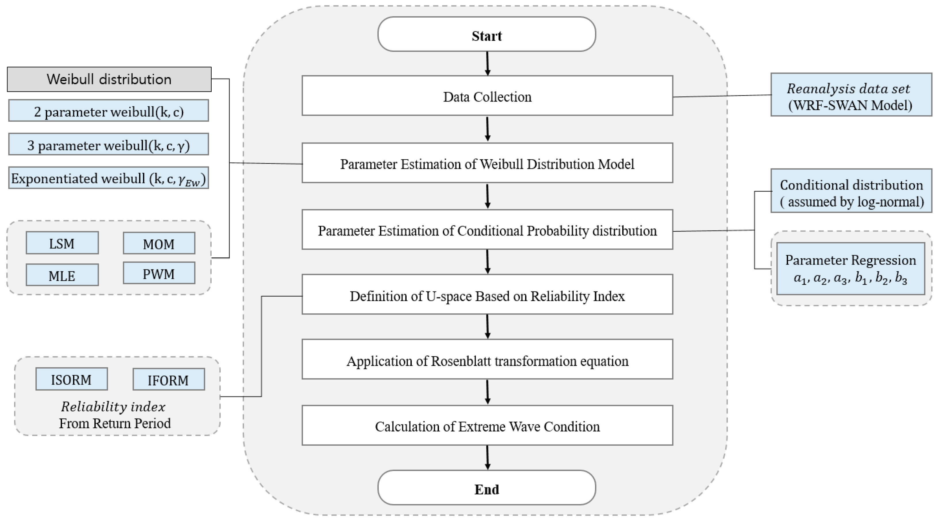
The process of estimating extreme wave conditions based on the joint distribution of significant wave height and peak period is illustrated in Figure 2. The procedure begins with the collection of long-term reanalysis data, followed by modeling the marginal distribution of significant wave height using various Weibull distributions. Parameters are estimated using several statistical techniques, including LSM, MLE, MOM, and probability weighted moment (PWM).

The conditional distribution of peak period corresponding to the significant wave height is assumed to follow a log-normal distribution. The conditional mean $\mathrm{E}\left[\ln \left(t_p\right)\right]$ and variance $\mathrm{V}\mathrm{A}\mathrm{R}\left[\ln \left(t_p\right)\right]$ are estimated using regression analysis.

A reliability index (β) corresponding to the target return period is used to define iso-probability contours in U-space. In this step, either the I-FORM or I-SORM can be applied, depending on whether a linear or second-order approximation of the limit state function is employed. Finally, the contour points are transformed back into the physical space, representing the extreme environmental conditions.

3.1. Weibull Distribution

The Weibull distribution is widely used in a number of fields, such as reliability analysis, lifetime prediction, quality control, and meteorological forecasting. In the wind energy industry in particular, it shows high fitness with the distributions of energy sources, such as waves, currents, and wind, and has been extensively applied to annual power generation prediction and extreme value analysis. We considered the 2-parameter, 3-parameter, and exponentiated Weibull distributions. The probability density function (PDF) and cumulative distribution function (CDF) of each distribution are shown in Equations (1)–(6).

$$f_{H_s}{\left(h_s\right)}_{2P}={\displaystyle \frac{k}{c}}{\left({\displaystyle \frac{h_s}{c}}\right)}^{k-1}·\mathrm{e}\mathrm{x}\mathrm{p}[-{\left({\displaystyle \frac{h_s}{c}}\right)}^k]$$

(1)

$$F_{H_s}{\left({\mathrm{h}}_s\right)}_{2P}=1-\mathrm{e}\mathrm{x}\mathrm{p}[-{\left({\displaystyle \frac{{\mathrm{h}}_s}{c}}\right)}^k]$$

(2)

$$f_{H_s}{\left(h_s\right)}_{3P}={\displaystyle \frac{k}{c}}{\left({\displaystyle \frac{h_s-\gamma }{c}}\right)}^{k-1}·\mathrm{e}\mathrm{x}\mathrm{p}[-{\left({\displaystyle \frac{h_s-\gamma }{c}}\right)}^k]$$

(3)

$$F_{H_s}{\left({\mathrm{h}}_s\right)}_{3P}=1-\mathrm{e}\mathrm{x}\mathrm{p}[-{\left({\displaystyle \frac{{\mathrm{h}}_s-\gamma }{c}}\right)}^k]$$

(4)

$$f_{H_s}{\left(h_s\right)}_{Exp}={\displaystyle \frac{{\gamma }_{Ew}k}{c}}{\left({\displaystyle \frac{h_s}{c}}\right)}^{k-1}·\mathrm{e}\mathrm{x}\mathrm{p}[-{\left({\displaystyle \frac{h_s}{c}}\right)}^k]·{\left\{1-[exp-{\left({\displaystyle \frac{h_s}{c}}\right)}^k]\right\}}^{{\gamma }_{Ew}-1}$$

(5)

$$F_{H_s}{\left({\mathrm{h}}_s\right)}_{\mathrm{E}\mathrm{x}\mathrm{p}}={\left\{1-exp[-{\left({\displaystyle \frac{h_s}{c}}\right)}^k]\right\}}^{{\gamma }_{Ew}}$$

(6)

where $k$, c, $\gamma$, and ${\gamma }_{Ew}$ are the shape, scale, location, and extra shape parameters, respectively, and h_s is the significant wave height. Shape parameter $k$ governs the steepness and symmetry of the distribution curve. Smaller k values result in broader and flatter distributions, whereas larger values result in narrower and more peaked profiles. The scale parameter $\mathrm{c}$ is proportional to the mean of the variable and controls the horizontal stretching of the distribution, reflecting the average intensity of the environmental conditions.

In the three-parameter Weibull distribution, the location parameter $\mathsf{\gamma }$ shifts the entire distribution to the right, facilitating the modeling of environmental variables, such as significant wave height, exhibiting a non-zero minimum threshold.

The extra shape parameter ${\mathsf{\gamma }}_{Ew}$ in the exponentiated Weibull distribution is an extended concept providing additional flexibility in capturing the asymmetry and tail behavior of the distribution, which cannot be fully represented by the shape parameter $k$ alone. Specifically, this parameter enables a more accurate modeling of tail characteristics frequently observed in marine environments.

These parameters are essential for constructing statistically flexible Weibull models responsive to site-specific oceanographic conditions. Here, combinations of these parameters were applied to build optimal Weibull models tailored to each offshore wind farm site.

3.2. Parameter Estimation

Here, LSM, MLE, MOM, and PWM were applied to estimate the Weibull distribution parameters. Each estimation method has different advantages and disadvantages depending on the characteristics of the data and the form of distribution, which can directly affect the accuracy of extreme value estimation.

Particularly, the MOM and PWM were applied only to 2- and 3-parameter Weibull distributions because their moment-based formulations were not compatible with those of the exponentiated Weibull model. In contrast, the MLE and LSM were used for all distribution types, including the exponentiated Weibull distribution.

3.2.1. Least Square Method

The LSM estimates parameters by linearly transforming observed data, with the advantages of simple calculations and fast convergence. In particular, the CDF of the Weibull distribution can be linearized through logarithmic transformation (Equation (7)), where the dependent variable y = $ln\left\{ln[{\displaystyle \frac{1}{1-F_{H_s}\left(h_s\right)}}]\right\}$ and the independent variable x = $\mathrm{l}\mathrm{n}{h}_s$ are defined for linear regression.

However, due to information loss occurring during the linear transformation process, limitations in accuracy persist; therefore, it is mainly used as an initial value for other parameter estimations.

$$ln\left\{ln[{\displaystyle \frac{1}{1-F_{H_s}\left(h_s\right)}}]\right\}=\mathrm{k}\mathrm{l}\mathrm{n}{h}_s-klnc$$

(7)

3.2.2. Maximum Likelihood Estimation

The MLE is the most widely used for estimating Weibull distribution parameters, providing statistically consistent estimates, especially for large datasets. However, when data are concentrated in low-wave regions, such as significant wave heights, the optimization process can be dominated by regions of high data density, potentially reducing the accuracy of extreme value estimation.

The MLE first defines the probability density function L (k, c) as shown in Equation (8) for the sample data (x₁, x₂, …, xₙ), and then converts it to the log-likelihood function as shown in Equation (9). This transformation simplifies the multiplication of probabilities into a summation of logarithmic terms, which is more tractable for differentiation. Subsequently, the optimal parameters are estimated by partially differentiating with respect to k and c to maximize the likelihood function [12,13].

$$L\left(k,c\right)=\prod _{i=1}^{n}f(x_i,k,c)=\prod _{i=1}^n{\displaystyle \frac{k}{c^k}}{x_i}^{k-1}exp (-{\left({\displaystyle \frac{x_i}{c}}\right)}^k)$$

(8)

$$lnL\left(k,c\right)=nlnk-nlnc-{\displaystyle \frac{1}{c^k}}\sum _{i=1}^n{x_i}^k+(k-1)\sum _{i=1}^{n}ln{x}_i$$

(9)

3.2.3. Method of Moment

The MOM is for estimating parameters under the assumption that the statistical moments (mean, variance, and skewness) of the sample data match those of the theoretical moments of the Weibull distribution. The parameters for the 2- and 3-parameter Weibull distributions were estimated sequentially using the first (mean), second (variance), and third (skewness) moments. The calculation process is relatively simple and intuitive; however, the use of higher-order moments increases sensitivity to extreme values, which can reduce the reliability of the estimation results in cases of asymmetric distributions or extreme values, such as marine environmental data. The theoretical mean (${\mathsf{\mu }}_{2P}$) and variance (${{\mathsf{\sigma }}^2}_{2P}$) of the 2-parameter Weibull distribution are given by Equations (10) and (11).

$${\mu }_{2P}=c\mathsf{\Gamma }(1+{\displaystyle \frac{1}{k}})$$

(10)

$${{\mathsf{\sigma }}_{2P}}^2=c^2\mathsf{\Gamma }\left(1+{\displaystyle \frac{2}{k}}\right)-{{\mu }_{2P}}^2$$

(11)

The theoretical mean (${\mathsf{\mu }}_{3P}$), variance (${{\mathsf{\sigma }}^2}_{3P}$), and skewness (${\mathrm{S}}_k$) of the 3-parameter Weibull distribution are given by Equations (12)–(14).

$${\mu }_{3P}=\gamma +c\mathsf{\Gamma }(1+{\displaystyle \frac{1}{k}})$$

(12)

$${{\mathsf{\sigma }}_{3P}}^2=c^2\left[\Gamma \left(1+{\displaystyle \frac{2}{k}}\right)-{\Gamma }^2(1+{\displaystyle \frac{1}{k}})\right]$$

(13)

$${\mathrm{S}}_{\mathrm{k}}=\sqrt{{\displaystyle \frac{{\left[\Gamma \left(1+\frac{3}{k}\right)-3\Gamma \left(1+\frac{1}{k}\right)\Gamma \left(1+\frac{2}{k}\right)+2{\Gamma }^3\left(1+\frac{1}{k}\right)\right]}^2}{{\left[\Gamma \left(1+\frac{2}{k}\right)-{\Gamma }^2\left(1+\frac{1}{k}\right)\right]}^3}}}$$

(14)

3.2.4. Probability Weighted Moment

The PWM follows the basic principles of MOM but improves the sensitivity to the tail of the distribution by assigning weights according to the rank of the data. Due to these characteristics, it can provide stable estimation results even for extreme value estimations or when data are concentrated in specific regions. It is particularly effective for asymmetric distributions with long tails, such as marine environmental data.

Using PWM, the CDF for a 3-parameter Weibull distribution of the sample data is defined by Equation (15) [14].

$$M_{p,r,s}={\int }_0^1{\left[x\left(F\right)\right]}^p{F}^r{(1-F)}^{s}dF$$

(15)

where $x\left(F\right)$ represents the inverse function of the CDF, and is defined by Equation (16).

$$x\left(F\right)=\gamma +{c[-\mathit{log}\left(1-F\right)]}^{{\displaystyle \frac{1}{k}}}$$

(16)

Substituting Equation (16) into Equation (15), the theoretical $M_{1,r,0}$ for the weighted probability moment for a 3-parameter Weibull distribution is defined by Equation (17), and the formulas for $M_r$ = $M_{1,r,0}$, r = 0, 1, 2 are given by Equations (18)–(20).

$$M_{1,r,0}=\gamma {\int }_0^1{F}^{r}dF+c{\int }_0^1{[-\mathit{log}\left(1-F\right)]}^{{\displaystyle \frac{1}{k}}}{F}^{r}dF$$

(17)

$$M_0=\gamma +c\mathsf{\Gamma }(1+{\displaystyle \frac{1}{k}})$$

(18)

$$M_1={\displaystyle \frac{\gamma }{2}}+(1-{\displaystyle \frac{1}{2^{1+\frac{1}{k}}}})c\mathsf{\Gamma }(1+{\displaystyle \frac{1}{k}})$$

(19)

$$M_2={\displaystyle \frac{\gamma }{3}}+(1-{\displaystyle \frac{1}{2^{1+\frac{1}{k}}}}+{\displaystyle \frac{1}{3^{1+\frac{1}{k}}}})c\mathsf{\Gamma }(1+{\displaystyle \frac{1}{k}})$$

(20)

The random sample mean ${\widehat{M_0}}_{(1,r,0)}$ and the first and second weighted moments ${\widehat{M_1}}_{(1,r,0)}$ and ${\widehat{M_2}}_{(1,r,0)}$ with weights assigned to the data ranks are defined by Equations (21)–(23) [15].

$${\widehat{M_0}}_{(1,r,0)}={\displaystyle \frac{1}{N}}\sum _{i=1}^N{x}_i$$

(21)

$${\widehat{M_1}}_{(1,r,0)}={\displaystyle \frac{1}{N(N-1)}}\sum _{i=1}^N(i-1)x_i$$

(22)

$${\widehat{M_2}}_{(1,r,0)}={\displaystyle \frac{1}{N(N-1)(N-2)}}\sum _{i=1}^{N-1}(i-1)(i-2)x_i$$

(23)

where $x_i$ and i represent a randomly sorted sample in ascending order and rank of that sample, respectively.

The sample mean ${\widehat{M_0}}_{(\mathrm{1,0},s)}$ and the first moment ${\widehat{M_1}}_{(\mathrm{1,0},s)}$ with weights assigned to the rank of the sample data for the 2-parameter Weibull distribution are given by Equations (24) and (25) [16].

$${\widehat{M_0}}_{(\mathrm{1,0},s)}={\displaystyle \frac{1}{N}}\sum _{i=1}^N{x}_i$$

(24)

$${\widehat{M_1}}_{(\mathrm{1,0},s)}={\displaystyle \frac{1}{N(N-1)}}\sum _{i=1}^{N-1}(n-i)x_i$$

(25)

since the 2-parameter Weibull distribution is a case where γ is 0, the parameters k and c are calculated from Equations (26) and (27) based on Equations (24) and (25).

$$k={\displaystyle \frac{ln\left(2\right)}{ln(\frac{{\widehat{M_0}}_{\left(\mathrm{1,0},s\right)}}{{\widehat{2M_1}}_{\left(\mathrm{1,0},s\right)}})}}$$

(26)

$$c={\displaystyle \frac{{\widehat{M_0}}_{\left(\mathrm{1,0},s\right)}}{\Gamma \left[\frac{\mathit{ln}\left(\frac{{\widehat{M_0}}_{\left(\mathrm{1,0},s\right)}}{{\widehat{M_1}}_{\left(\mathrm{1,0},s\right)}}\right)}{\mathit{ln}\left(2\right)}\right]}}$$

(27)

3.3. Environmental Contour Method

The EC method is a reliability-based design approach that efficiently approximates extreme environmental conditions and is used in various fields, such as marine structure design, extreme environment prediction, and environmental load risk assessment. The EC method derives extreme design conditions by transforming multidimensional probability distributions into iso-probability surfaces.

The joint probability distribution, $f_{H_s{T}_P}\left(h_s,t_p\right),$ can be expressed as the product of the marginal probability distribution of the significant wave height $f_{H_s}\left(h_s\right)$ and the conditional probability distribution of the peak period $f_{\left.T_p\right|H_s}\left(t_p|h_s\right)$, as shown in Equation (28).

$$f_{H_s{T}_P}\left(h_s,t_p\right)=f_{H_s}\left(h_s\right)f_{\left.T_p\right|H_s}\left(t_p|h_s\right)$$

(28)

Here, to model the joint probability distribution, the Weibull distribution was applied to the marginal probability distribution of the significant wave height, as shown in Equation (29), and the log-normal distribution was applied to the conditional probability distribution of the peak period corresponding to the significant wave height, as shown in Equation (30):

$$f_{H_s}\left(h_s\right)={\displaystyle \frac{k}{c}}{\left({\displaystyle \frac{h_s}{c}}\right)}^{k-1}exp\left[-{({\displaystyle \frac{h_s}{c}})}^k\right]$$

(29)

$$f_{\left.T_p\right|H_s}\left(t_p|h_s\right)={\displaystyle \frac{1}{t_p\sigma \sqrt{2\pi }}}exp\left[{\displaystyle \frac{{-(\mathit{ln}\left(t_p\right)-\mu )}^2}{2{\sigma }^2}}\right]$$

(30)

where k, c, μ, and ${\sigma }^2$ represent shape parameter, scale parameter, mean, and variance, respectively, and when 3-parameter Weibull or exponentiated Weibull distribution models are applied, parameters γ or ${\gamma }_{Ew}$ are added.

The conditional probability distribution parameters are determined by the conditional mean $E[\mathit{ln}\left(t_p\right)]$ and variance $VAR[\mathit{ln}\left(t_p\right)]$, which are defined by Equations (31) and (32), respectively. Here, a₁, a₂, a₃ and b₁, b₂, b₃ are coefficients determining the conditional mean and variance, respectively [17,18].

$$E[\mathit{ln}\left(t_p\right)]=\mu =a_1+a_2·{h_s}^{a_3}$$

(31)

$$VAR[\mathit{ln}\left(t_p\right)]={\sigma }^2=b_1+b_2·\mathrm{e}\mathrm{x}\mathrm{p}[-h_s·b_3]$$

(32)

In extreme value estimation for two variables, both I-FORM and I-SORM have the same process of transforming physical space variables into independent variable space (U-space) through Rosenblatt transformation but differ in the way they approximate the limit state surface. I-FORM calculates the reliability index by linearly approximating the limit state surface, whereas I-SORM calculates the reliability index (β) by considering the curvature of the limit state surface through second-order approximation. In bivariate problems, the reliability index of the I-SORM is calculated using a two-dimensional chi-square distribution considering the principal curvature of the limit state surface, resulting in more conservative extreme values than those of the I-FORM under the same exceedance probability [19].

3.4. Goodness of Fit Assessment

We performed a quantitative analysis and visual verification to evaluate the parameter estimation of Weibull distributions and the suitability of extreme models. Goodness-of-fit tests for Weibull distribution parameter estimation include the Kolmogorov–Smirnov (K–S) test, root mean square error (RMSE), and mean absolute error (MAE). The K–S test examines the fitness between distributions based on the maximum difference in the cumulative distribution functions; however, it has limitations in evaluating the overall fitness of the distribution. The MAE, calculated as the average of the absolute errors, tends to be less sensitive to large deviations compared to RMSE. Here, RMSE, which can effectively evaluate the average error magnitude across the entire data range, was adopted to quantitatively assess the distribution fitness. RMSE is defined by Equation (33) [20].

$$RMSE=\sqrt{{\displaystyle \frac{1}{N}}\sum _{i=1}^N{(V_{mod,i}-V_{obs,i})}^2}$$

(33)

where N is the number of data points, V_mod is the CDF value of the estimated distribution function, and V_obs is the empirical CDF value of the actual observed data.

In extreme value analysis, accurate modeling of the tail region of the distribution is crucial. Accordingly, the exceedance probability was log-transformed to evaluate the fitness of the tail region of the distribution. This method has the advantage of effectively visualizing the probability of extreme events and intuitively evaluating the degree of agreement between the estimated distribution and the observed data in the tail region.

Additionally, a quantile estimation method based on exceedance probability was applied to evaluate the reliability of the extreme models. The relative position value of the sample data was defined using the exceedance probability and data count, and the marginal empirical return value was calculated using linear interpolation. The estimation accuracy across various return periods was comprehensively evaluated by comparing the marginal empirical return value corresponding to the exceedance probability of a specific return period with that of the extreme value estimated by the EC method using the RMSE.

4. Results and Discussion

4.1. Weibull Distribution Parameter Estimation

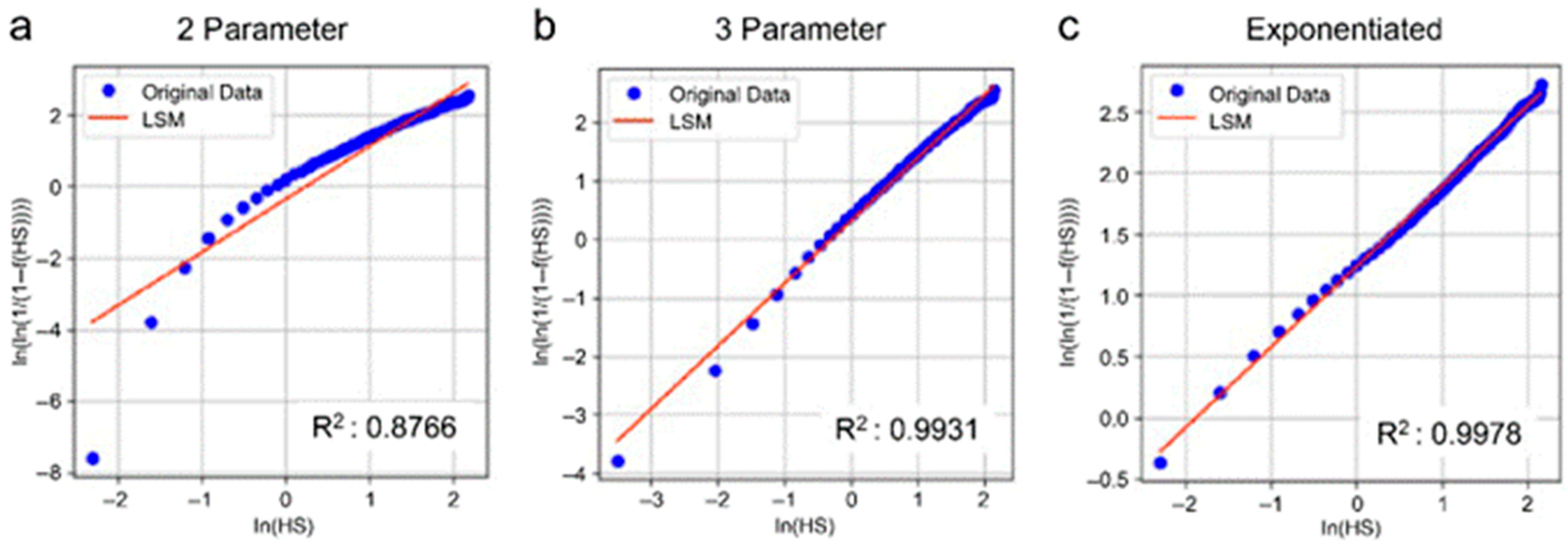
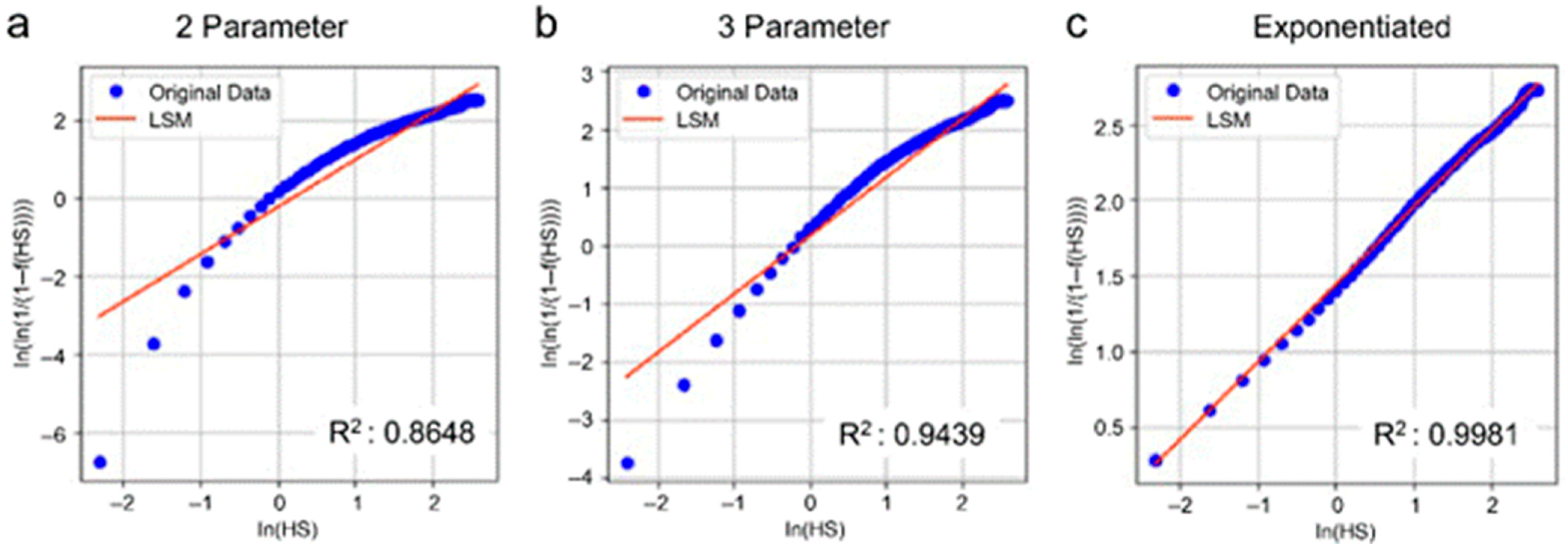
The LSM, MLE, MOM, and PWM were applied to estimate the Weibull distribution parameters. Figure 3, Figure 4, Figure 5 and Figure 6 present the LSM fitting results for two-parameter, three-parameter, and exponentiated Weibull distribution models for the Shinan, Chujado, Yokjido, and Ulsan sea areas.

The initial fitness evaluation using the coefficient of determination (R²) shows that the exponentiated Weibull distribution model had the highest R² values for all sea areas. The results calculated by the LSM were used as the initial values for the MLE, MOM, and PWM.

Table 3. Estimated Weibull parameters for each site.

Location		LSM-2P	LSM-3P	LSM-Exp	MLE-2P	MLE-3P	MLE-Exp	MOM-2P	MOM-3P	PWM-2P	PWM-2P
Shinan	k	1.47	1.08	0.75	1.45	1.14	0.48	1.31	0.99	1.44	0.97
	c	1.15	0.72	0.25	0.93	0.72	0.05	0.91	0.64	0.92	0.62
	$\gamma$	-	0.16	-	-	0.16	-	-	0.19	-	0.21
	${\gamma }_{Ew}$	-	-	5.01	-	-	20.2	-	-	-	-
Chujado	k	1.49	1.13	0.66	1.54	1.33	0.64	1.41	0.99	1.56	1.04
	c	1.28	0.82	0.15	0.97	0.83	0.15	0.95	0.61	0.96	0.65
	$\gamma$	-	0.14	-	-	0.11	-	-	0.25	-	0.22
	${\gamma }_{Ew}$	-	-	10.1	-	-	9.99	-	-	-	-
Yokjido	k	1.11	0.66	0.51	1.60	1.22	0.51	1.48	0.87	1.65	1.14
	c	1.05	0.26	0.06	1.00	0.75	0.06	0.99	0.50	1.00	0.70
	$\gamma$	-	0.44	-	-	0.21	-	-	0.36	-	0.22
	${\gamma }_{Ew}$	-	-	21.9	-	-	22.5	-	-	-	-
Ulsan	k	1.74	1.11	0.65	1.78	1.35	0.63	1.70	1.05	1.85	1.26
	c	1.82	0.92	0.17	1.25	0.94	0.16	1.24	0.71	1.24	0.88
	$\gamma$	-	0.25	-	-	0.26	-	-	0.41	-	0.29
	${\gamma }_{Ew}$	-	-	14.9	-	-	14.5	-	-	-	-

Abbreviations: LSM, least squares method; MLE, maximum likelihood estimation; MOM, method of moment; PWM, probability weighted moment; 2P, 2-parameter; 3P, 3-parameter; Exp, exponentiated.

lists the parameters calculated using each estimation method.

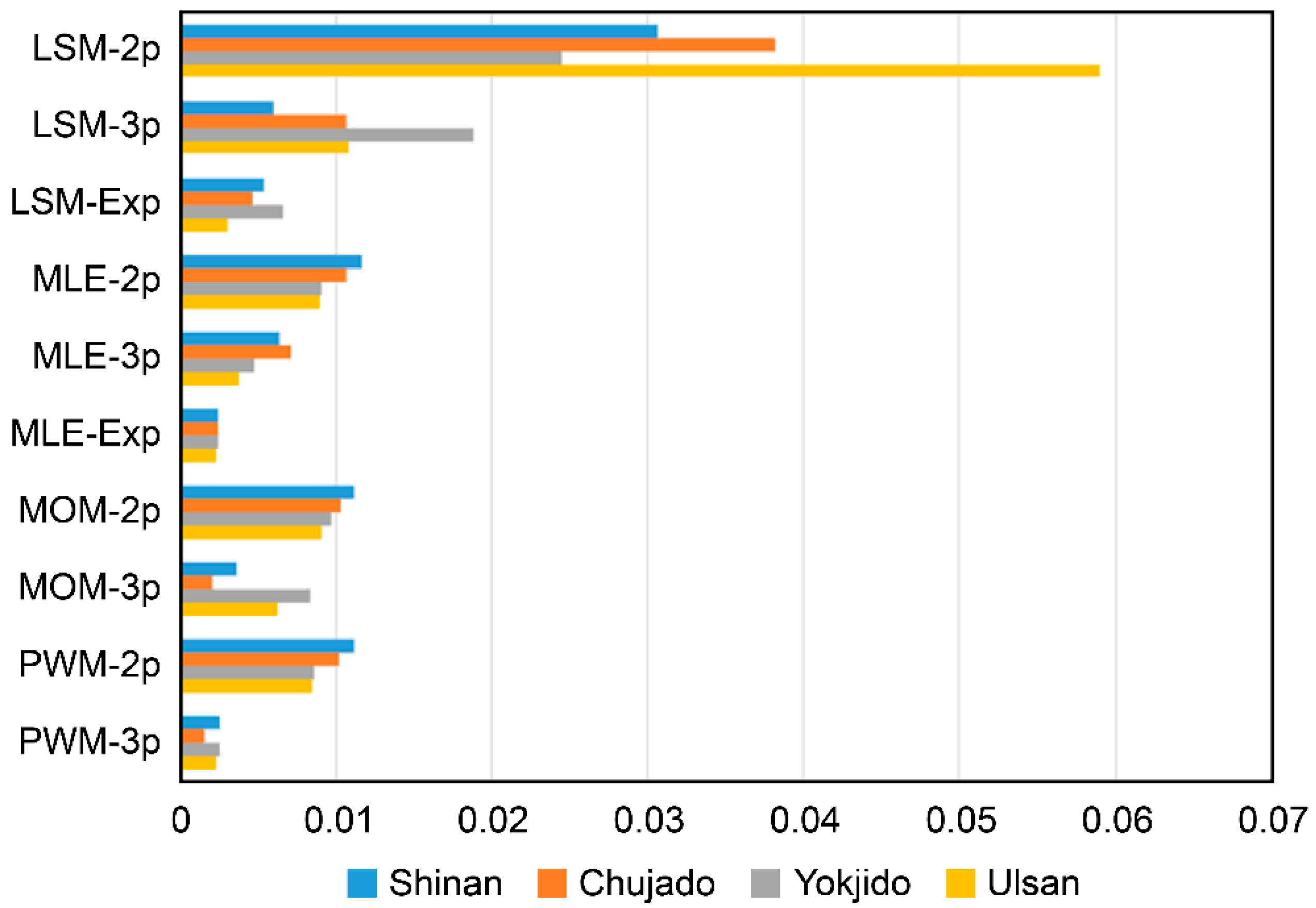
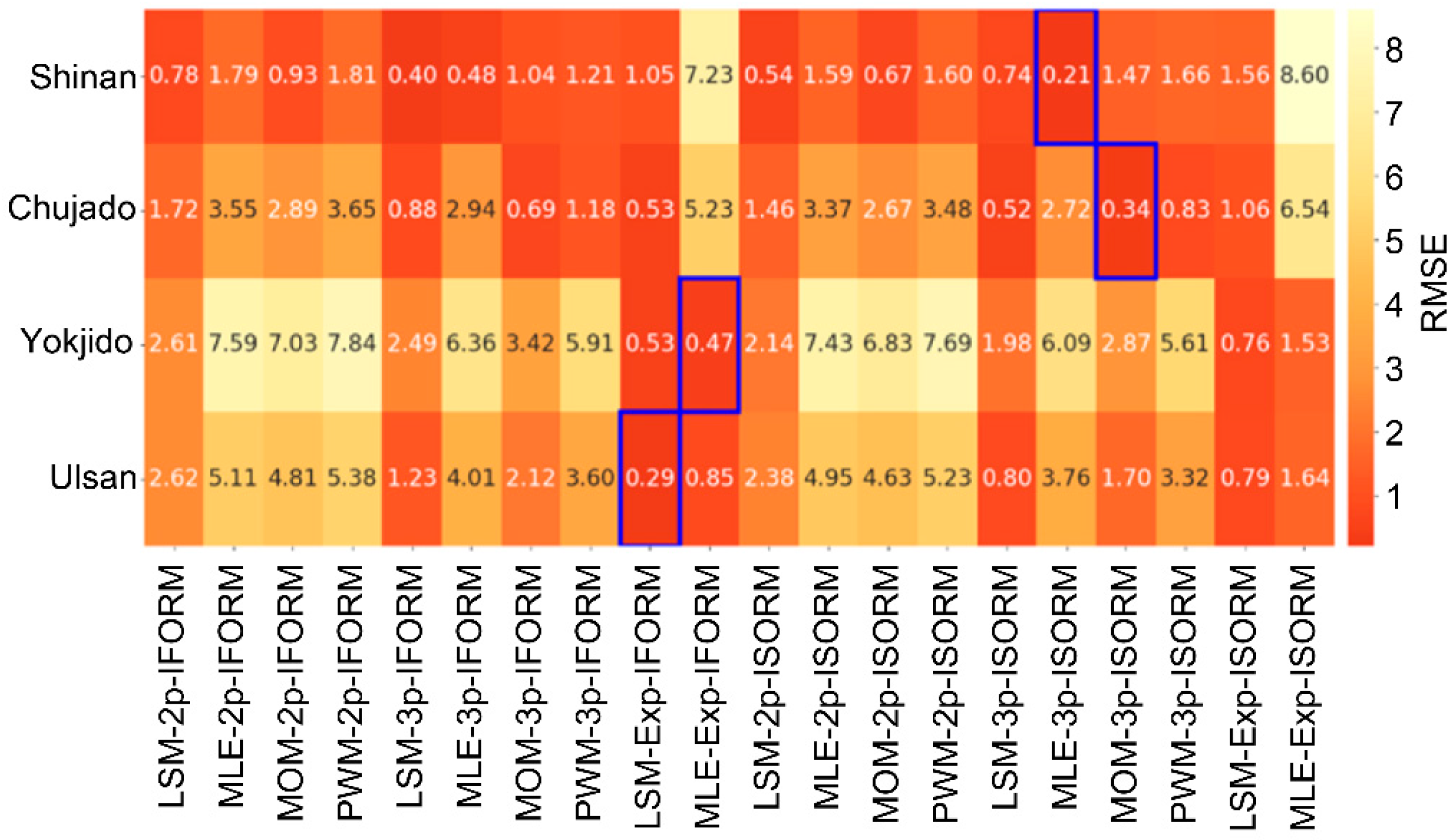
To evaluate the fitness of parameter estimation, the RMSE was calculated by applying various estimation methods for each sea area (Figure 7), and the ranking of parameter estimation methods based on RMSE values is shown in

Table 4. Root mean square error (RMSE)-based ranking for parameter estimation methods.

Location	LSM 2P	LSM 3P	LSM Exp	MLE 2P	MLE 3P	MLE Exp	MOM 2P	MOM 3P	PWM 2P	PWM 3P
Shinan	10	5	4	9	6	1	8	3	7	2
Chujado	10	9	4	8	5	3	7	2	6	1
Yokjido	10	9	4	7	3	1	8	5	6	2
Ulsan	10	9	3	7	4	1	8	5	6	2

. The results show that the MLE-Exp and PWM-3P of the Weibull model performed well in all sea areas. This can be attributed to the fact that the additional extra shape parameter ${\gamma }_{Ew}$ of the exponentiated Weibull distribution improves the flexibility of the probability density function, and MLE and PWM each comprise robust estimation characteristics for large samples. However, LSM showed a relatively high RMSE due to the information loss occurring during the linear transformation process, and the 2P Weibull distribution showed limitations in capturing complex probability distribution characteristics due to restricted parameter structure.

Figure 8 shows the results of converting the exceedance probability to a logarithmic scale to evaluate the tail region fitness of the Weibull distributions. The analysis reveals that the quality of fit in the tail region varies significantly across the four sea areas. In the Shinan area, the combination of LSM-3P and MLE-3P yielded superior fits, whereas in the Chujado area, MOM-3P and LSM-Exp performed the best. The MLE-Exp and LSM-Exp combinations exhibited the highest tail region fit for the Yokjido and Ulsan regions.

These outcomes are attributed to the interaction between the mathematical characteristics of each parameter estimation method and the site-specific frequency and distribution of extreme events. Particularly, in tail analysis, applying a uniform estimation technique across all sites may not be appropriate; instead, selecting an optimal combination tailored to each location is essential.

The fit of the tail region did not necessarily align with the overall fit, as assessed by the RMSE. For example, in Yokjido and Ulsan, both MLE-Exp and PWM-3P showed strong performance across the full distribution and tail region. However, considerable discrepancies were observed between the two domains in the Shinan and Chujado areas. This suggests the need to independently consider the overall distribution and tail region in extreme value analysis, and particularly in extreme value estimation; an approach that prioritizes selecting distribution combinations with superior tail fitness and reflecting them in EC methods is more reasonable.

Such regional variations are largely influenced by the distinct marine environmental conditions of each area, such as coastal bathymetry, prevailing wind and wave patterns, and current dynamics, which directly affect the occurrence and behavior of extreme wave events. Therefore, site-specific modeling reflecting these environmental conditions is crucial for enhancing the reliability of extreme value estimations.

4.2. Reliability Analysis of Extreme Value Estimation

A quantile estimation method based on exceedance probability was adopted to objectively evaluate the accuracy of extreme value estimation. This approach has the advantage of comprehensively evaluating the estimation accuracy of extreme values across various return periods. The optimal statistical techniques for each sea area were identified by comparing the RMSE of the marginal empirical return values—derived from exceedance probabilities across multiple return periods—with those estimated using the EC method, as illustrated in Figure 9. Based on a comprehensive framework combining various Weibull distribution forms, parameter estimation techniques, and EC methods, 20 combinations were tested per site to ensure a robust and thorough performance evaluation.

In the Shinan sea area, the MLE-3P combination using I-SORM showed the best performance, with an RMSE of 0.21. For the Chujado area, the combination of I-SORM and MOM-3P provided optimal results with an RMSE of 0.34. In contrast, the I-FORM approach was more effective for the Yokjido and Ulsan sea areas, where the MLE-Exp and LSM-Exp combinations provided the lowest RMSE values of 0.47 and 0.29, respectively.

On the other hand, some combinations showed significantly inferior performance, with RMSE values exceeding 5.0 in certain cases. For example, the MLE-Exp using I-SORM in both the Shinan and Chujado areas exhibited particularly poor performance. Likewise, the PWM-2P combined with I-FORM yielded the lowest accuracy for the Yokjido and Ulsan sites. A summary of the best- and worst-performing combinations for each site is presented in

Table 5. Best and worst-performing statistical combinations by site.

Site	Best Method	RMSE	Worst Method	RMSE
Shinan	I-SORM + MLE-3P	0.21	I-SORM + MLE-Exp	8.60
Chujado	I-SORM + MOM-3P	0.34	I-SORM + MLE-Exp	6.54
Yokjido	I-FORM + MLE-Exp	0.47	I-FORM + PWM-2P	7.84
Ulsan	I-FORM + LSM-Exp	0.29	I-FORM + PWM-2P	5.38

. These findings emphasize the critical need to select statistical models that are tailored to site-specific environmental conditions, as different combinations of EC methods and estimation techniques exhibit optimal performance across different regions.

As shown in the tail behavior analysis (Figure 8), the rate of tail decay plays a critical role in determining the suitability of I-FORM and I-SORM for each region. For the Shinan and Chujado sea areas, which exhibit rapid tail decay, I-SORM—accounting for the curvature of the limit state surface—demonstrated superior performance. Conversely, for Yokjido and Ulsan, where the tail decay is more gradual, sufficient estimation accuracy was achieved using I-FORM, which relies on linear approximation.

These results suggest that applying one-size-fits-all statistical methods to extreme wave analyses may be inappropriate. For reliable extreme analysis, it is essential to select customized EC methods and statistical techniques fully considering the characteristics of the target sea area. The multi-faceted verification methodology presented here is significant in that it provides objective criteria for selecting extreme analysis models that consider regional characteristics.

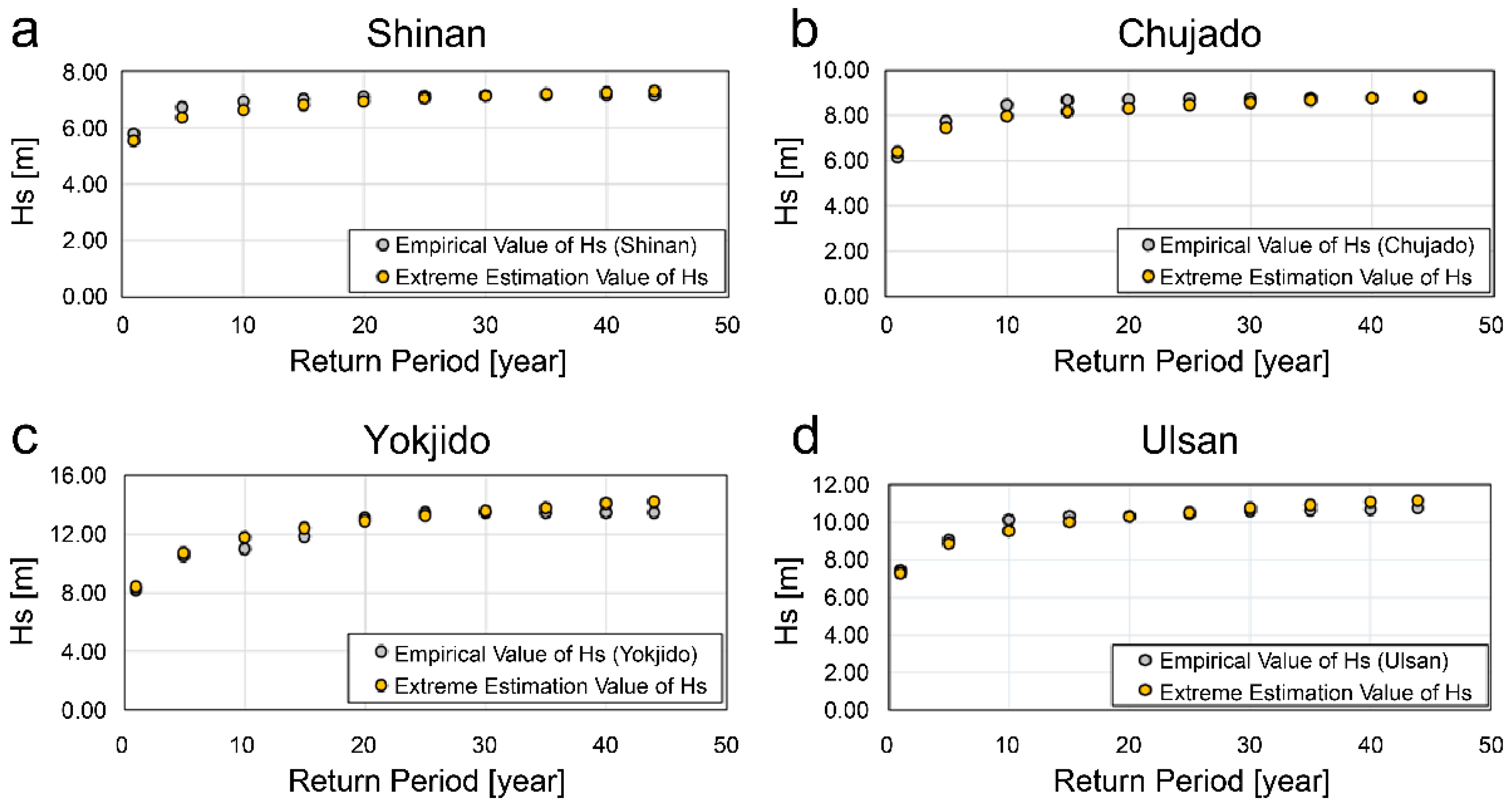
Figure 10 shows a comparison of the marginal empirical return value by return period and the extreme values estimated by optimal statistical techniques for each sea area. Figure 11, Figure 12, Figure 13 and Figure 14 present EC with a 44-year return period, the same as those of the sample data collection period, for each sea area.

4.3. Result of Extreme Design Wave

Floating offshore wind systems operate when exposed to various external environmental conditions such as wind, waves, and currents. Accordingly, optimal design must consider the environmental characteristics of the installation site. Among these, wave loads have a particularly dominant influence on the dynamic response and motion behavior of structures, acting as key contributors to structural stress and fatigue.

International standards IEC61400-3-2 [9] and DNV-ST-0119 (2018 edition) [10] define the return periods of extreme design waves as 1, 50, 100, and 500 years for the stable operation of offshore wind systems. In accordance with these standards, we calculated extreme design wave by applying optimal statistical techniques derived for each promising candidate site for South Korean offshore wind farms, and the results are presented in

Table 6. Extreme wave design for potential offshore wind farms in South Korea.

Return Period (Year)	Shinan		Chujado		Yokjido		Ulsan
	Hs (m)	Tp (s)	Hs (m)	Tp (s)	Hs (m)	Tp (s)	Hs (m)	Tp (s)
1	5.51	9.94	6.39	9.70	8.35	11.32	7.27	10.19
50	7.34	11.79	8.89	11.49	14.41	15.66	11.29	12.29
100	7.67	12.10	9.33	11.79	15.65	16.42	12.07	12.67
500	8.40	12.81	10.36	12.48	18.26	18.16	13.93	13.52

.

5. Conclusions

This study proposed a methodological framework to enhance the accuracy of EC-based extreme wave predictions by leveraging the observed correlation between tail behavior and the performance of various statistical estimation techniques. To further improve the reliability of extreme value estimation, a quantile estimation approach based on exceedance probability was also introduced as part of the framework evaluation.

The optimal combination of statistical models varied by site, reflecting region-specific differences in the tail characteristics of wave distributions. Furthermore, the results confirm that the accuracy of extreme value estimation strongly depends on how well the statistical model captures tail behavior and how appropriately the EC method is selected and applied in accordance with those characteristics.

The proposed framework was validated using data from four representative offshore sites in South Korea and is readily extendable to other regions where long-term observational records or high-resolution hindcast datasets are available. While this study primarily focused on I-FORM and I-SORM, future research should incorporate comparative evaluations involving alternative EC methods—such as direct FORM, highest density contour (HDC), and inverse directional simulation (IDS)—to improve the framework’s generalizability and applicability.

Overall, the proposed framework can make a significant contribution to the development of practical design standards that enhance both structural safety and cost-efficiency in marine renewable energy systems.