Abstract
Robots with multiple degrees of freedom (DOFs), such as underwater vehicle–manipulator systems (UVMSs), are expected to optimize system performance by exploiting redundancy with various basic tasks while still fulfilling the primary objective. Multiple tasks for robots, which are expected to be carried out simultaneously with prescribed priorities, can be referred to as sets of tasks (SOTs). In this work, a hybrid vision/force control method with continuous task transitions is proposed for a UVMS to simultaneously track the reference vision and force trajectory during manipulation. Several tasks with expected objectives and specific priorities are established and combined as SOTs in hybrid vision/force tracking. At different stages, various SOTs are carried out with different emphases. A hierarchical optimization-based whole-body control framework is constructed to obtain the solution in a strictly hierarchical fashion. A continuous transition method is employed to mitigate oscillations during the task switching phase. Finally, comparative simulation experiments are conducted and the results verify the improved convergence of the proposed tracking controller for UVMSs.
1. Introduction
Exploring and utilizing ocean resources has become a matter of strategic importance around the world against the backdrop of global resource scarcity. Underwater equipment is being increasingly investigated given the rising demands of underwater operations [1]. The underwater vehicle–manipulator system (UVMS), which is composed of an underwater vehicle and manipulator(s), is designed to expand the capacity and enhance the functionality of underwater operations. However, the attached manipulator(s) increases the complexity of the system, which brings new challenges in terms of whole-system design, multibody kinematics and dynamics and convoluted control algorithms [2]. Significant efforts have been devoted to developing a reliable and valuable UVMS that can operate in harsh underwater conditions.
Precise trajectory tracking control is the key technology to improve the autonomy of UVMSs. Generally, the control algorithms of UVMSs are mainly classified into two main categories. In the most straightforward sense, the control algorithms of the main vehicle and the manipulator are implemented for the corresponding degrees of freedom (DOFs) independently. In [3], the authors combined a standard proportional–integral–differential (PID) control with a prior model to track the desired vehicle velocity, while a cascade joint controller was employed to control the velocity and angle of each joint. This approach does not consider the couplings, so the system performance is necessarily limited. In improved methods, the dynamic couplings between the vehicle and manipulator are treated as disturbances and handled by feedforward compensation [4]. In [5], the authors discussed the coupling property and proposed a Slotine sliding mode approach to reduce the coupling effect. Active compensation is implemented in the control law to counteract the undesirable effect by measuring or estimating the interaction force from the manipulator in [6]. In general, the simplicity of this approach makes it attractive, and some control techniques from manipulators [7,8] and unmanned aerial vehicles (UAVs) [9] can be readily referenced and transferred. However, the main vehicle will usually be designed to be much heavier than the attached manipulator(s), resulting in relatively smaller reactive forces from the manipulator(s) compared to the vehicle’s own weight, as in the Phoenix+SMART3S [2].
Another control scheme is to model the vehicle and the attached manipulator(s) as a serial chain of rigid bodies by regarding the UVMS as a whole system. However, more challenges will arise due to the increased complexity of the whole system, such as inaccurate parameters of the hydrodynamic effects, kinematic redundancy of the system, etc.
Several classical control methodologies have been successfully applied to trajectory tracking in UVMSs, including robust PID in [10,11,12,13,14], sliding mode control (SMC) in [15,16,17,18] and adaptive controllers in [19,20,21,22,23], which are capable of effectively addressing external disturbances and unmodeled dynamics. Furthermore, advanced nonlinear control strategies, such as control in [24,25], prescribed performance control in [26,27] and neural network techniques in [28,29,30,31], have also been implemented to control underwater vehicles. However, these methods demonstrate limited capabilities in handling state constraints. Consequently, model predictive control (MPC) has been extensively adopted due to its inherent constraint handling advantages in the field of underwater vehicles, as shown in [32,33,34,35,36].
The previously mentioned works focus on tracking the trajectory based on the position, which is difficult to measure accurately in the underwater environment. Vision sensors are an important means of localization in a GPS-denied environment, which is referred to as visual servoing; this has also been widely used in underwater vehicles for dynamic positioning [37,38], path following [39], docking [40,41] and underwater manipulation [42,43].
The capacity to handle interactions is one of the fundamental requirements to accomplish the manipulation task successfully [44]. The contact force at the manipulator’s end-effector is employed to describe the state of interaction. Thus, force control strategies are often employed in scenarios where a robot intervenes in the environment, and they can be classified into ’direct force control’ and ’indirect force control’ according to whether the force is controlled directly or not [45]. Both of them are mainly constructed based on position control schemes and have been widely used for fixed-base manipulators.
However, the velocity and position of free-floating robots are difficult to measure accurately and rapidly, making it challenging to practically implement force control algorithms for freely moving manipulators [46], in which even higher precision and update rates are necessitated than in position control. Therefore, the current force control studies on mobile robots, including wheeled mobile robots [47,48,49] and UAVMs [50,51], remain largely confined to laboratory environments, with limited real-world applications. The same situation applies to UVMSs, including both impedance control ([52,53]) and direct force control ([54,55,56]).
In line with the distinction between position-based visual servoing (PBVS) and image-based visual servoing (IBVS), force control strategies can also bypass the reconstruction of the position and directly regulate contact forces using visual information. In image-based force control, the translational positions are replaced by visual features; then, visual features and forces are simultaneously tracked in a unique control law to handle the interaction with the environment. A vision-based impedance force control algorithm was introduced for a laboratory injection system in [57]. The injection force was estimated by utilizing visual feedback via the concept of visual–force integration. Meanwhile, three types of hybrid visual–impedance control schemes that directly relate image feature errors to external forces by projecting the force component onto the image plane were proposed in [58]. This approach enables stable physical interaction between an unmanned aerial manipulator and its task environment.
Challenges also arise from the complexity of handling multiple DOFs in the whole UVMS system. A set of tasks (SOT) is expected to be carried out simultaneously with prescribed priorities by utilizing the redundant DOFs of the UVMS. Task-based control methods for UVMSs have been proposed in [59,60,61] with the consideration of priorities between tasks. In [62], a whole-body control (WBC) framework for a dual-arm UVMS is proposed to deal with multidimensional inequality control objectives. In this work, WBC is firstly introduced for the controller of the UVMS. Although it is similar to some task-priority-based control methods, it offers a distinct perspective on the problem by utilizing the whole system’s DOFs.
Considering the advantages of IBVS, a vision-based force control task is established without the position reconstruction process. By employing image moments instead of point features, this method achieves enhanced robustness. Furthermore, a multitask framework considering smooth transitions can preserve the priority of the force tracking task while effectively mitigating fluctuations.
In our previous work, an image-based visual serving method for UVMSs was introduced [42]. The hierarchical control architecture is composed of a kinematic model predictive IBVS controller and a dynamic velocity controller, respectively. In this work, a whole-body vision/force control framework is proposed to simultaneously track the reference vision and force trajectory, which fully exploits the whole-body DOFs of the UVMS. The contributions of this work are summarized as follows:
- A whole-body multitask control framework is proposed to simultaneously accomplish the visual trajectory tracking and contact force tracking of a UVMS. This approach allows flexible task combinations in different scenarios while consistently maintaining strict priorities.
- By reprojecting the image points and choosing proper image moment combinations, decoupled visual features aligned along the tangential and normal directions of the target plane can be obtained, which enhances the independence among individual tasks.
- A continuous transition method for SOT switching is presented to optimize the performance in the transition process, particularly by effectively reducing fluctuations in the contact force.
This paper is organized as follows. The system formulation and visual servo model are introduced in Section 2. Several tasks for hybrid vision/force control based on WBC are established and a hierarchical WBC framework is reviewed in Section 3. In Section 4, a continuous transition method for SOT switching in WBC is proposed. The simulation results are demonstrated in Section 5. Lastly, we draw the conclusions of our paper and discuss further research problems.
2. System Model and Problem Statement
In this part, the whole system and the modeling process of the UVMS are first reviewed. Then, the contact model and the visual servo model for the hybrid vision/force control are introduced as the research basis.
2.1. UVMS Model
This work focuses on the control and analysis of a free-floating UVMS attached with an n-link manipulator. In Figure 1, the schematic provides an illustration of the system and frame definitions. The notations of the relevant frames are listed in Table 1.

Figure 1.
System model.

Table 1.
The notations of frames.
The modeling process of the UVMS follows the approach described in [2], in which the system is regarded as a serial chain of rigid bodies with hydrodynamics. In this part, a brief summary is provided for completeness, including the kinematics and the dynamics. The global pose vector of the UVMS is defined as
including the position vector ; the orientation vector , described by the Euler angle; and the joint vector , representing the joint angles of the manipulator with n joints.
The following equation defines the kinematics of the UVMS:
where is the system velocity vector, consisting of the body-fixed linear velocity , the body-fixed angular velocity of the base vehicle and the joint velocity . is the rotation matrix expressing the transformation from the body-fixed frame to the inertial frame, and is a Jacobian matrix describing the connection between and .
Define as the pose vector of the end-effector in the inertial frame I, where is the position and is the orientation in quaternion form. According to [2], we have
where and are the end-effector velocities expressed in the I-frame, and is the mapping matrix, which maps the -dimensional velocities into 6-dimensional end-effector velocities.
Remark 1.
The system is redundant as , which means that kinematic redundancy can be exploited to achieve additional task(s) besides the expected end-effector task.
The velocity of the end-effector in the reference frame E is defined as . Then, the relationship between and can be obtained by
where is the rotation matrix expressing the transformation from the inertial frame I to the E frame.
In the underwater environment, the total forces and moments acting on the generic part of the serial chain, including hydrodynamics, can be derived. Then, we write them in matrix form, and the dynamic equation of the UVMS is given by
where and are the inertia and coriolis/centripetal matrices considering the additional mass influences from hydrodynamic effects, and represents the linear and quadratic damping matrix. is the restoring force vector due to gravity and buoyancy. is the vector of the control inputs, including the vehicle control input and joint torque vector . and are the external contact force and disturbance force expressed in the inertial frame, respectively. The global pose vector , the system velocity and the control input are constrained as
where and are the lower and upper bounds of the corresponding variables.
2.2. Contact Model
An object–environment contact model describes the relationship between the contact force and the deformation, which is a very complex physical process. In [63], a stiffness-damping environmental model with a satisfactory matching degree is used, as shown in Figure 2.
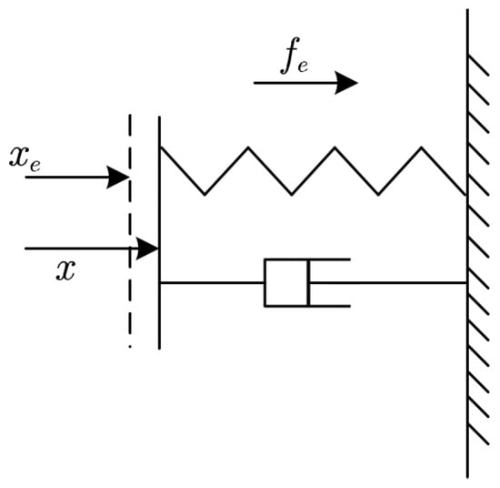
Figure 2.
Environmental contact model.
The dynamic relationship is simplified as
where and are the damping and stiffness coefficients; x and are the actual position and the equilibrium position, respectively; and f is the contact force.
2.3. Modeling of Visual Servo System
Image moments are selected as visual features due to the favorable decoupling characteristics. To further isolate the force control task from visual servo tasks, an image reprojection technique is employed by projecting the image points onto a virtual image plane that is always parallel to the target plane.
The detailed reprojection process can be found in [36] and is omitted here. For any image point, its original pixel coordinate is represented by and its reprojected coordinate in frame A is written as . Considering that N virtual image points constitute a visual target on the virtual image plane, we can define the image feature vector
where , and are three normalized image moments ([64]) calculated form the central moments.
Given that the virtual camera frame and the target frame are always aligned, it is easy to obtain the body-fixed velocity of frame A by
and the rotation matrix between frame C and A is given by
The dynamic relationship between and the relative motion of frame A and frame C can be described by
where is the velocity of the virtual camera in the reference frame A, including the linear velocity and angular velocity , and is the velocity of the real camera. is the interaction matrix, which is defined as
It is clear that shows good decoupling characteristics between the three translational motions, and the image moments computed from the reprojected image are fully decoupled.
Since the camera is fixed on the end-effector, the relationship between the camera velocity and the end-effector velocity can be obtained by the velocity Jacobian matrix
with
where is the skew-symmetric matrix operator, and is the position vector of the camera relative to the end-effector in frame E.
By substituting (4), (9) and (13) into (11), the derivative of visual features and the system velocity can be connected by
where is the Jacobian matrix of .
2.4. Problem Statement
The control objective of this work is to simultaneously track the reference visual trajectory of the UVMS while maintaining a desired contact force with the target plane.
3. Vision/Force Hybrid Control for UVMSs
A hybrid vision/force control framework based on WBC for UVMSs is established in this part. The operation is decomposed into several tasks, and a hierarchical optimization-based WBC is established to construct a unified output among the tasks.
3.1. Hybrid Vision/Force Control Tasks for UVMS
The general definition of one task includes the generic task variable and its corresponding Jacobian matrix relating its time derivative to the system velocity . Then, the differential relationship is given by
where the subscript indicates the variable related to the task notation. Thus, the task is accomplished by finding the appropriate to track the reference , which is a simple inverse kinematic (IK) problem, as (15) is defined at the kinematic level. However, these tasks are not only limited to IK; they can also be employed at the dynamic level.
In our work, the tasks in hybrid vision/force tracking for UVMSs will be defined as follows.
3.1.1. End-Effector Orientation
The orientation of the end-effector is represented in unit quaternion form, and the task of end-effector orientation is implemented as
where and are the reference value and the state error of the orientation of the end-effector. The quaternion error is calculated by , with the advantage of using the end-effector angular velocity and the corresponding orientation Jacobian extracted from [2]. is the positive control gain.
3.1.2. End-Effector Trajectory of UVMS
Visual servoing is employed to track the reference trajectory of the end-effector. The tangential movement of the end-effector to the target plane is described by and the task is defined as
The normal motion is connected with and controlled separately because it is highly coupled with the contact force in the normal direction of the plan, and the task of will be defined later.
3.1.3. Normal Contact Force
The contact force in normal direction is considered in this work. The reprojection process also has the advantage of allowing the use of the Jacobian matrix of ; then, the control task is obtained.
Only one of the two tasks of and in the same direction will be activated at the same time.
3.1.4. Main Vehicle Attitude Holding
In most cases, the main vehicle is preferably kept horizontal because of the requirements of the attached sensors (e.g., Doppler velocity logger (DVL), camera). By defining and the corresponding Jacobian , a horizontal attitude holding task is considered.
3.1.5. Camera’s Field of View
The image features are constrained states limited by the camera’s field of view (FOV), which is an inequality-constrained task. The indirect method is to convert the unequal constraints into equal tasks. Considering any one constrained state , its lower-bound rejection task can be formulated as
where is the safe buffer and means that the task is deactivated when unnecessary. In the same way, the upper-bound rejection task is defined as
The constraint is ensured by an equation task. It is clear that expressing such tasks via inequalities is more intuitive:
For convenience, the task is defined as , including the Jacobian matrix and the expected lower and upper derivatives ( in a task of equal constraints). For two tasks and , if has a higher priority than , it is called ; otherwise, . In a hierarchical controller, N tasks with the priority of are combined into an SOT, , and deployed to accomplish the whole mission collectively.
3.2. Hierarchical Optimization-Based Whole-Body Control
One single task is a simple inverse kinematic problem, which can be solved using a pseudo-inverse matrix. Then, when considering n tasks with different priorities, a closed-form WBC based on null space projection can find a solution that always satisfies the hierarchy, but it can only handle equal constraints. To deal with unequal constraints, an optimization-based WBC (OWBC) will be constructed.
Generally, the problem can be expressed in a general optimization-based form:
Then, when considering n tasks with different priorities, a weighting matrix can be added to the optimization problem to ensure the precedence rules:
where
are the corresponding Jacobian matrices and states of these tasks, and
consists of the weighing matrices of the tasks.
To obtain the solution to an optimization problem in a strictly hierarchical manner, a hierarchical optimization-based WBC (HWBC) can be formulated as in the following recursive optimization problem.
From , the optimization problem is constructed and solved in recursive form:
s.t.
where are the slack variables obtained after solving the first k task, and and are the lower and the upper constraints of task n. The implementation in accordance with the condensed procedure is shown in Algorithm 1.
| Algorithm 1 HWBC for UVMS |
| Input: Initial SOT of UVMS: ; |
| Output: Reference value: ; |
| Initialization: ={}; |
| for each do |
| Set and initialize the optimization problem (42); |
| Solve the optimization problem and obtain ; |
| Compute the slack variable ; |
| ; |
| end for |
| return ; |
4. Continuous and Smooth Task Transitions for Vision/Force Control
If does not change in the working process, the hierarchical controller can be solved based on the proposed HWBC. However, in practical operations, the controller needs to incorporate different SOTs at different stages, e.g., tasks being added or removed, priorities changing, etc. If directly switches to , the control output may oscillate. Inspired by the continuous transition approach in [65], a smooth transition method for SOT switching in hybrid vision/force control for UVMSs is proposed in this part, which is called continuous HWBC (CWBC).
4.1. Task Addition/Removal
Consider a single task that will be inserted into with the priority of , in which with switches to with . The transition method can be expressed as
s.t.
where is the transition coefficient from 0 to 1. When , Equation (45c) becomes
in which has the same solution as . Moreover, with , which indicates the end of the transition process. By increasing from 0 to 1 during the transition, the feasible solution area of will be moved to continuously and smoothly. The implementation of (44) is described in Algorithm 2.
| Algorithm 2 CWBC for UVMS: Adding a Task |
| Input: Initial SOT of UVMS: , task to be added: ; |
| Output: Reference value: ; |
| 1: if is empty() then |
| 2: Initialization: ; |
| 3: end if |
| 4: Solve: ; |
| 5: Set transition tasks: |
| ; |
| 6: Set transition SOT for : |
| ; |
| 7: Solve: ; |
| 8: Update: ; |
| 9: if then |
| 10: End of transition; |
| 11: end if |
| 12: return ; |
The transition coefficient can be computed by a nonlinear activation function with respect to the start time of the period.
4.2. Task Priority Swapping
Considering two existing tasks and with the priority of in , the following swapping process will be constructed:
s.t.
where is still the transition coefficient from 0 to 1, and is the solution of when (48c) and (48d) are set as
while is the solution of when (48c) and (48d) become
The implementation of (47) is described in Algorithm 3.
| Algorithm 3 CWBC for UVMS: Switching Task Priorities |
| Input: Initial SOT of UVMS , task to be switched: and ; |
| Output: Reference value: |
| 1: if is empty() then |
| 2: Initialization: ; |
| 3: end if |
| 4: Set transition tasks: ; |
| 5: Set transition SOT for : ; |
| 6: Solve: ; |
| 7: Set transition tasks: ; |
| 8: Set transition SOT for : ; |
| 9: Solve: ; |
| 10: Set transition tasks: ; |
| 11: Set transition tasks: ; |
| 12: Set transition SOT for : ; |
| 13: Solve: ; |
| 14: Update: ; |
| 15: if then |
| 16: End of transition; |
| 17: end if |
| 18: return ; |
5. Simulation Results
In this section, a visualized numerical simulation is conducted to evaluate the proposed controller. The system dynamics and control algorithm are calculated by MATLAB (version: R2024b), and the simulation visualization is performed by CoppeliaSim, as shown in Figure 3. The model of the main vehicle is based on the Kambara underwater vehicle model in [66], and a sway thruster is added to the thrust mapping matrix to render the vehicle fully actuated. The parameters of the attached manipulator can be seen in Appendix A. The links are assumed to be symmetric cylinders to simplify the calculation of the hydrodynamic forces, and the details can be found in the SIMURV 4.1 paper [2]. The optimization problem is solved by the open-source solver CasADi in [67].
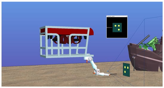
Figure 3.
Visualized simulation.
The dynamic velocity controller is detailed in [42]. To verify the robustness of the controller, we apply a time-varying external force on the end-effector of the UVMS as a disturbance and add a 10% error to the model parameters. The external force is set as in the inertial frame. The parameters of the contact model are set as , and , and Gaussian white noise of 10 db is added in the force measurement in the simulation.
Two common cases that require contact force tracking are considered in this section. One involves maintaining a contact force with a fixed point, such as button pressing. The other requires maintaining the desired contact force while moving the contact point, such as welding or flaw detection. The simulation is conducted based on these two cases.
The tasks for the hybrid vision/force control mission are listed in Table 2. Depending on whether task is active or not, the SOTs are defined as and .
Table 2.
Task list.
5.1. Fixed Contact Case
A reference trajectory for the end-effector in the fixed contact case is considered in this part. The initial states of the UVMS are set as
and the fixed reference states are
The results of the fixed contact case based on OWBC and the proposed CWBC are shown in Figure 4, Figure 5, Figure 6, Figure 7 and Figure 8. Overall, both of the controllers are capable of driving the end-effector to the desired point and maintaining a stable contact force.
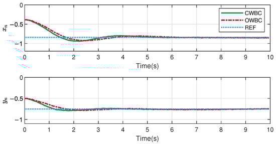
Figure 4.
Tangential image moments.
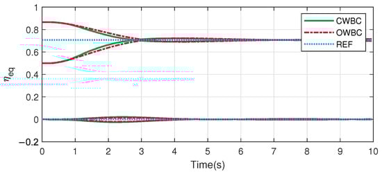
Figure 5.
End-effector quaternions.
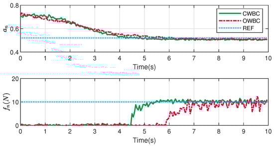
Figure 6.
Normal image moment and contact force.
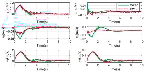
Figure 7.
Velocities of main vehicle.
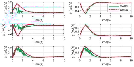
Figure 8.
Joint velocities.
The image moments in the tangential directions of the target plane and the end-effector quaternions are demonstrated in Figure 4 and Figure 5. It can be observed that both the tangential image moments and the end-effector quaternions exhibit similar performance for the two controllers.
The main difference is reflected in the normal direction in Figure 6. After task is introduced into the SOT at about 4 s by , the contact force of CWBC in green converges to the reference value more quickly and stably than the red curve of OWBC. Although the force control tasks are the same in the two controllers, the better performance comes from the strictly hierarchical priorities in CWBC.
The system velocities are demonstrated in Figure 7 and Figure 8. It can be observed that CWBC exhibits greater fluctuations in the velocities of the main vehicle, whereas OWBC shows larger fluctuations in joint motions. This results from the fact that OWBC does not impose strict task prioritization, and its performance aligns more closely with the overall energy consumption by moving the joint in the first place.
5.2. Moving Contact Case
A circular reference trajectory for the UVMS is considered and designed as
and the other conditions are the same as in Section 5.1. The results are shown in Figure 9, Figure 10, Figure 11, Figure 12 and Figure 13. The contact condition between the environment and the end-effector is subjected to change in order to evaluate the controller’s adaptability to different situations during the tracking process, which is achieved by changing the equilibrium position and stiffness coefficient to and .
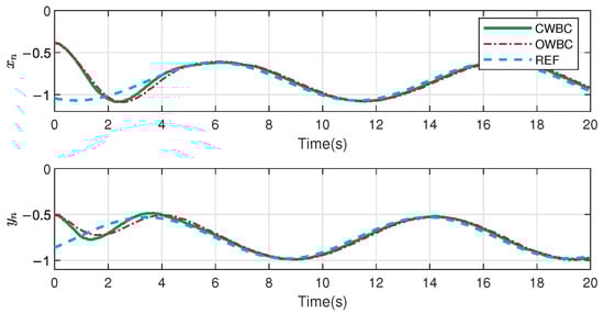
Figure 9.
Tangential image moments.
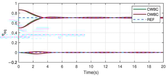
Figure 10.
End-effector quaternions.
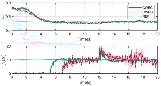
Figure 11.
Normal image moment and contact force.
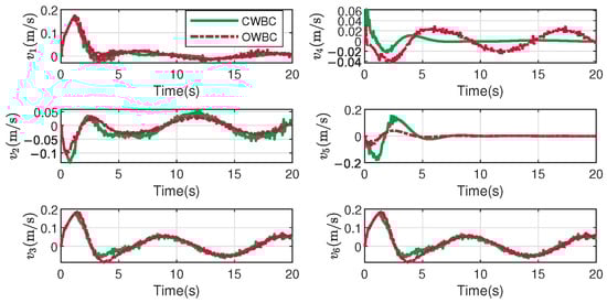
Figure 12.
Velocities of main vehicle.
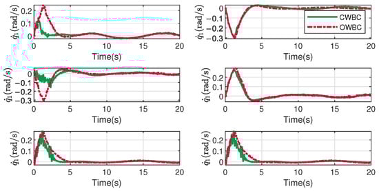
Figure 13.
Joint velocities.
In the moving case, similar performance can be seen, as shown in Figure 9 and Figure 10. One can notice that there is little difference between the curves of the tangential image moments and the end-effector quaternions for the two controllers.
The normal image moment and contact force curves are shown in Figure 11. Although both of the controllers can maintain the reference force, thanks to the strict priority of the force control task, the result of CWBC is obviously better than that of OWBC, with fewer fluctuations. At about 12 s, the normal contact forces suddenly increase when the contact condition changes and then gradually stabilize to the expected value. The adaptability of the two controllers can be certified.
Figure 12 and Figure 13 exhibit the results regarding the system velocities. The difference between the velocities of the main vehicle and the joint velocities remains similar to that described in Section 5.1, in which CWBC shows greater fluctuations from the main vehicle movements and OWBC shows larger fluctuations in joint motions.
5.3. Parameter Selection
The control performance of the proposed CWBC controller under different control gains in the force control task is demonstrated in this part to show the selection process of the control gains. All the initial and reference states remain consistent with those specified in Section 5.1. The fixed contact case is repeated three times with different : Case 1 with , Case 2 with and Case 3 with .
The results of the three cases are shown in Figure 14. It can be observed that the the performances differs notably. Specifically, Case 2 demonstrates slow tracking performance accompanied by gradual fluctuations, while Case 3 achieves fast tracking at the cost of noticeable oscillations. In general, the control force of Case 1 achieves balanced overall performance in terms of tracking speed and fluctuations.
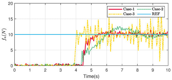
Figure 14.
Contact force with different parameters.
5.4. Comparative Results
A comparison of to via smooth transitions with CWBC and by direct switching with HWBC is demonstrated in this part. The reference trajectory and parameters are the same as in Section 5.2, without contact condition changes, and the results are shown in Figure 15 and Figure 16.
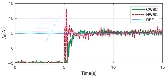
Figure 15.
Contact force.
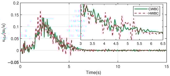
Figure 16.
Velocity of end-effector in x direction.
The contact forces are shown in Figure 15. In general, both of the curves converge to the desired values stably under the two controllers, while the two methods exhibit different behaviors during the transition phase. The force result in HWBC shows larger fluctuations, whereas CWBC approaches the desired value more smoothly. Significant fluctuations are observed in the velocity along the force control direction in Figure 16, which is consistent with the variation in the contact force. This demonstrates the effectiveness of the smooth transition method in CWBC to optimize the switching performance when the force control task is introduced in the SOT.
The root mean square error (RMSE), settling time (ST) and overshoot (OS) of the two controllers are demonstrated in Table 3. The RMSE and the ST are relatively close, indicating that the convergence rates of the two controllers are similar. A notable distinction between the two controllers is observed in the OS. The OS of CWBC is 1.8 (N), while the OS of HWBC is 8.1 (N). This is not only reflected in the improved tracking performance but is particularly critical in intervention tasks, as excessive overshoot of the contact force could potentially lead to system damage or instability.
Table 3.
Result comparison.
6. Conclusions
In this paper, we have proposed a whole-body vision/force controller to complete the manipulation task of a UVMS. A HVS model based on reprojecting image moments and quaternions was firstly established. Then, several tasks were constructed to establish a hybrid vision/force control framework for UVMSs, and a HWBC framework was constructed to generate a solution that satisfied the priorities. To obtain a smooth output during the transition phrase, a continuous transition for SOT switching is presented. Simulation results verify the excellent performance and robustness of the proposed hybrid vision/force controller. In the near future, we will integrate trajectory planning into the controller and try to conduct real-world experiments.
Author Contributions
Conceptualization, J.L. and J.G.; Data curation, G.C.; Formal analysis, G.C.; Funding acquisition, F.Z.; Investigation, J.G.; Methodology, J.L.; Project administration, F.Z.; Software, J.L.; Supervision, J.G.; Validation, G.C. and J.G.; Visualization, J.L.; Writing—original draft, J.L.; Writing—review and editing, G.C. and J.G. All authors have read and agreed to the published version of the manuscript.
Funding
This work was supported by the National Natural Science Foundation of China under Grant 51979228.
Institutional Review Board Statement
Not applicable.
Informed Consent Statement
Not applicable.
Data Availability Statement
Data are contained within the article.
Conflicts of Interest
The authors declare no conflicts of interest. The funders had no role in the design of the study; in the collection, analyses, or interpretation of the data; in the writing of the manuscript; or in the decision to publish the results.
Abbreviations
The following abbreviations are used in this manuscript:
| UVMS | Underwater Vehicle–Manipulator System |
| DOF | Degree of Freedom |
| SOT | Set of Tasks |
| WBC | Whole-Body Control |
| OWBC | Optimization-Based WBC |
| HWBC | Hierarchical Optimization-Based WBC |
| CWBC | Continuous HWBC |
Appendix A. Manipulator Parameters
Table A1.
DH parameters.
Table A1.
DH parameters.
| Num. | a [m] | d [m] | [rad] | [rad] |
|---|---|---|---|---|
| link 1 | 0.075 | 0 | ||
| link 2 | 0.305 | 0 | 0 | |
| link 3 | 0.055 | 0 | ||
| link 4 | 0 | 0.305 | ||
| link 5 | 0 | −0.057 | ||
| link 6 | 0 | 0.222 | 0 |
The links are assumed to be symmetric cylinders to simplify the calculation of the hydrodynamic forces; the link parameters of the manipulator are listed in Table A2.
Table A2.
Link parameters.
Table A2.
Link parameters.
| Num. | Mass [kg] | Radius [m] | Length [m] | Viscous Friction [Nms] |
|---|---|---|---|---|
| link 1 | 5 | 0.08 | 0.15 | 30 |
| link 2 | 8 | 0.08 | 0.35 | 20 |
| link 3 | 4 | 0.08 | 0.15 | 5 |
| link 4 | 4 | 0.06 | 0.45 | 10 |
| link 5 | 4 | 0.06 | 0.1 | 5 |
| link 6 | 3 | 0.05 | 0.25 | 6 |
References
- Song, J.; He, X. Robust state estimation and fault detection for autonomous underwater vehicles considering hydrodynamic effects. Control Eng. Pract. 2023, 135, 105497. [Google Scholar] [CrossRef]
- Antonelli, G. Underwater Robots; Springer: Berlin/Heidelberg, Germany, 2018; Volume 123. [Google Scholar]
- Youakim, D.; Ridao, P.; Palomeras, N.; Spadafora, F.; Ribas, D.; Muzzupappa, M. Moveit!: Autonomous underwater free-floating manipulation. IEEE Robot. Autom. Mag. 2017, 24, 41–51. [Google Scholar] [CrossRef]
- Sivčev, S.; Coleman, J.; Omerdić, E.; Dooly, G.; Toal, D. Underwater manipulators: A review. Ocean Eng. 2018, 163, 431–450. [Google Scholar] [CrossRef]
- Dannigan, M.; Russell, G.T. Evaluation and reduction of the dynamic coupling between a manipulator and an underwater vehicle. IEEE J. Ocean Eng. 1998, 23, 260–273. [Google Scholar] [CrossRef]
- Ryu, J.-H.; Kwon, D.-S.; Lee, P.-M. Control of underwater manipulators mounted on an rov using base force information. In Proceedings of the 2001 ICRA, IEEE International Conference on Robotics and Automation (Cat. No. 01CH37164), Seoul, Republic of Korea, 21–26 May 2001; IEEE: New York, NY, USA, 2001; Volume 4, pp. 3238–3243. [Google Scholar]
- Tian, G.; Tan, J.; Li, B.; Duan, G. Optimal fully actuated system approach-based trajectory tracking control for robot manipulators. IEEE Trans. Cybern. 2024, 54, 7469–7478. [Google Scholar] [CrossRef]
- Wang, F.; Chen, K.; Zhen, S.; Chen, X.; Zheng, H.; Wang, Z. Prescribed performance adaptive robust control for robotic manipulators with fuzzy uncertainty. IEEE Trans. Fuzzy Syst. 2023, 32, 1318–1330. [Google Scholar] [CrossRef]
- Xiong, J.-J.; Chen, Y. Rbfnn-based parameter adaptive sliding mode control for an uncertain tquav with time-varying mass. Int. J. Robust Nonlinear Control 2025, 35, 4658–4668. [Google Scholar] [CrossRef]
- Han, J.; Chung, W.K. Active use of restoring moments for motion control of an underwater vehicle-manipulator system. IEEE J. Ocean Eng. 2013, 39, 100–109. [Google Scholar] [CrossRef]
- Esfahani, H.N.; Azimirad, V.; Danesh, M. A time delay controller included terminal sliding mode and fuzzy gain tuning for underwater vehicle-manipulator systems. Ocean Eng. 2015, 107, 97–107. [Google Scholar] [CrossRef]
- Londhe, P.; Mohan, S.; Patre, B.; Waghmare, L. Robust task-space control of an autonomous underwater vehicle-manipulator system by pid-like fuzzy control scheme with disturbance estimator. Ocean Eng. 2017, 139, 1–13. [Google Scholar] [CrossRef]
- Martin, S.C.; Whitcomb, L.L. Nonlinear model-based tracking control of underwater vehicles with three degree-of-freedom fully coupled dynamical plant models: Theory and experimental evaluation. IEEE Trans. Control Syst. Technol. 2017, 26, 404–414. [Google Scholar] [CrossRef]
- David, J.; Bauer, R.; Seto, M. Coupled hydroplane and variable ballast control system for autonomous underwater vehicle altitude-keeping to variable seabed. IEEE J. Ocean Eng. 2017, 43, 873–887. [Google Scholar] [CrossRef]
- Patre, B.M.; Londhe, P.S.; Waghmare, L.M.; Mohan, S. Disturbance estimator based non-singular fast fuzzy terminal sliding mode control of an autonomous underwater vehicle. Ocean Eng. 2018, 159, 372–387. [Google Scholar] [CrossRef]
- Lakhekar, G.; Waghmare, L. Adaptive fuzzy exponential terminal sliding mode controller design for nonlinear trajectory tracking control of autonomous underwater vehicle. Int. J. Dyn. Control 2018, 6, 1690–1705. [Google Scholar] [CrossRef]
- Liu, X.; Zhang, M.; Chen, J.; Yin, B. Trajectory tracking with quaternion-based attitude representation for autonomous underwater vehicle based on terminal sliding mode control. Appl. Ocean. Res. 2020, 104, 102342. [Google Scholar] [CrossRef]
- Liu, X.; Zhang, M.; Yang, C.; Yin, B. Finite-time tracking control for autonomous underwater vehicle based on an improved non-singular terminal sliding mode manifold. Int. J. Control 2022, 95, 840–849. [Google Scholar] [CrossRef]
- Sun, Y.C.; Cheah, C.-C. Adaptive setpoint control of underwater vehicle-manipulator systems. In Proceedings of the IEEE Conference on Robotics, Automation and Mechatronics, Singapore, 1–3 December 2004; IEEE: New York, NY, USA, 2004; Volume 1, pp. 434–439. [Google Scholar]
- Antonelli, G.; Caccavale, F.; Chiaverini, S. Adaptive tracking control of underwater vehicle-manipulator systems based on the virtual decomposition approach. IEEE Trans. Robot. Autom. 2004, 20, 594–602. [Google Scholar] [CrossRef]
- Vito, D.D.; Palma, D.D.; Simetti, E.; Indiveri, G.; Antonelli, G. Experimental validation of the modeling and control of a multibody underwater vehicle manipulator system for sea mining exploration. J. Field Robot. 2021, 38, 171–191. [Google Scholar] [CrossRef]
- Antonelli, G.; Cataldi, E. Recursive adaptive control for an underwater vehicle carrying a manipulator. In Proceedings of the 22nd Mediterranean Conference on Control and Automation, Palermo, Italy, 16–19 June 2014; IEEE: New York, NY, USA, 2014; pp. 847–852. [Google Scholar]
- Li, J.; Huang, H.; Wan, L.; Zhou, Z.; Xu, Y. Hybrid strategy-based coordinate controller for an underwater vehicle manipulator system using nonlinear disturbance observer. Robotica 2019, 37, 1710–1731. [Google Scholar] [CrossRef]
- Han, J.; Park, J.; Chung, W.K. Robust coordinated motion control of an underwater vehicle-manipulator system with minimizing restoring moments. Ocean Eng. 2011, 38, 1197–1206. [Google Scholar] [CrossRef]
- Dai, Y.; Yu, S. Design of an indirect adaptive controller for the trajectory tracking of UVMS. Ocean Eng. 2018, 151, 234–245. [Google Scholar] [CrossRef]
- Heshmati-Alamdari, S.; Bechlioulis, C.P.; Karras, G.C.; Nikou, A.; Dimarogonas, D.V.; Kyriakopoulos, K.J. A robust interaction control approach for underwater vehicle manipulator systems. Annu. Rev. Control 2018, 46, 315–325. [Google Scholar] [CrossRef]
- Lin, Z.; Wang, H.D.; Karkoub, M.; Shah, U.H.; Li, M. Prescribed performance based sliding mode path-following control of UVMS with flexible joints using extended state observer based sliding mode disturbance observer. Ocean Eng. 2021, 240, 109915. [Google Scholar] [CrossRef]
- Xu, B.; Pandian, S.R.; Sakagami, N.; Petry, F. Neuro-fuzzy control of underwater vehicle-manipulator systems. J. Frankl. Inst. 2012, 349, 1125–1138. [Google Scholar] [CrossRef]
- Gao, J.; An, X.; Proctor, A.; Bradley, C. Sliding mode adaptive neural network control for hybrid visual servoing of underwater vehicles. Ocean Eng. 2017, 142, 666–675. [Google Scholar] [CrossRef]
- Li, X.; Zhu, D. An adaptive som neural network method for distributed formation control of a group of auvs. IEEE Trans. Ind. Electron. 2018, 65, 8260–8270. [Google Scholar] [CrossRef]
- Huang, H.; Li, J.; Zhang, G.; Tang, Q.; Wan, L. Adaptive recurrent neural network motion control for observation class remotely operated vehicle manipulator system with modeling uncertainty. Adv. Mech. Eng. 2018, 10, 1687814018804098. [Google Scholar] [CrossRef]
- Shen, C.; Shi, Y.; Buckham, B. Integrated path planning and tracking control of an auv: A unified receding horizon optimization approach. IEEE/ASME Trans. Mechatron. 2016, 22, 1163–1173. [Google Scholar] [CrossRef]
- Li, H.; Yan, W. Model predictive stabilization of constrained underactuated autonomous underwater vehicles with guaranteed feasibility and stability. IEEE/Asme Trans. Mechatron. 2016, 22, 1185–1194. [Google Scholar] [CrossRef]
- Dai, Y.; Yu, S.; Yan, Y.; Yu, X. An ekf-based fast tube mpc scheme for moving target tracking of a redundant underwater vehicle-manipulator system. IEEE/ASME Trans. Mechatron. 2019, 24, 2803–2814. [Google Scholar] [CrossRef]
- Wei, H.; Shen, C.; Shi, Y. Distributed lyapunov-based model predictive formation tracking control for autonomous underwater vehicles subject to disturbances. IEEE Trans. Syst. Man, Cybern. Syst. 2019, 51, 5198–5208. [Google Scholar] [CrossRef]
- Liu, J.; Gao, J.; Yan, W. Lyapunov-based model predictive visual servo control of an underwater vehicle-manipulator system. IEEE Trans. Intell. Veh. 2024. early access. [Google Scholar] [CrossRef]
- Gao, J.; Proctor, A.; Bradley, C. Adaptive neural network visual servo control for dynamic positioning of underwater vehicles. Neurocomputing 2015, 167, 604–613. [Google Scholar] [CrossRef]
- Krupínski, S.; Allibert, G.; Hua, M.-D.; Hamel, T. An inertial-aided homography-based visual servo control approach for (almost) fully actuated autonomous underwater vehicles. IEEE Trans. Robot. 2017, 33, 1041–1060. [Google Scholar] [CrossRef]
- Allibert, G.; Hua, M.-D.; Krupínski, S.; Hamel, T. Pipeline following by visual servoing for autonomous underwater vehicles. Control Eng. Pract. 2019, 82, 151–160. [Google Scholar] [CrossRef]
- Park, J.-Y.; Jun, B.-h.; Lee, P.-m.; Oh, J. Experiments on vision guided docking of an autonomous underwater vehicle using one camera. Ocean Eng. 2009, 36, 48–61. [Google Scholar] [CrossRef]
- Myint, M.; Yonemori, K.; Lwin, K.N.; Yanou, A.; Minami, M. Dual-eyes vision-based docking system for autonomous underwater vehicle: An approach and experiments. J. Intell. Robot. Syst. 2018, 92, 159–186. [Google Scholar] [CrossRef]
- Gao, J.; Liang, X.; Chen, Y.; Zhang, L.; Jia, S. Hierarchical image-based visual serving of underwater vehicle manipulator systems based on model predictive control and active disturbance rejection control. Ocean Eng. 2021, 229, 108814. [Google Scholar] [CrossRef]
- Huang, H.; Bian, X.; Cai, F.; Li, J.; Jiang, T.; Zhang, Z.; Sun, C. A review on visual servoing for underwater vehicle manipulation systems automatic control and case study. Ocean Eng. 2022, 260, 112065. [Google Scholar] [CrossRef]
- Siciliano, B.; Sciavicco, L.; Villani, L.; Oriolo, G. Force Control; Springer: Berlin/Heidelberg, Germany, 2009. [Google Scholar]
- Ott, C.; Mukherjee, R.; Nakamura, Y. Unified impedance and admittance control. In Proceedings of the 2010 IEEE International Conference on Robotics and Automation, Anchorage, AK, USA, 3–7 May 2010; IEEE: New York, NY, USA, 2010; pp. 554–561. [Google Scholar]
- Ridao, P.; Carreras, M.; Ribas, D.; Sanz, P.J.; Oliver, G. Intervention auvs: The next challenge. Annu. Rev. Control 2015, 40, 227–241. [Google Scholar] [CrossRef]
- Li, Z.; Ge, S.S.; Ming, A. Adaptive robust motion/force control of holonomic-constrained nonholonomic mobile manipulators. IEEE Trans. Syst. Man, Cybern. Part B (Cybern.) 2007, 37, 607–616. [Google Scholar] [CrossRef] [PubMed]
- Ali, M.A.; Radzak, M.S.; Mailah, M.; Yusoff, N.; Razak, B.A.; Karim, M.S.A.; Ameen, W.; Jabbar, W.A.; Alsewari, A.A.; Rassem, T.H.; et al. A novel inertia moment estimation algorithm collaborated with active force control scheme for wheeled mobile robot control in constrained environments. Expert Syst. Appl. 2021, 183, 115454. [Google Scholar] [CrossRef]
- Rani, S.; Kumar, A.; Kumar, N.; Singh, H.P. Adaptive robust motion/force control of constrained mobile manipulators using rbf neural network. Int. J. Dyn. Control 2024, 12, 3379–3391. [Google Scholar] [CrossRef]
- Malczyk, G.; Brunner, M.; Cuniato, E.; Tognon, M.; Siegwart, R. Multi-directional interaction force control with an aerial manipulator under external disturbances. Auton. Robot. 2023, 47, 1325–1343. [Google Scholar] [CrossRef]
- Meng, X.; He, Y.; Han, J.; Song, A. Physical interaction oriented aerial manipulators: Contact force control and implementation. IEEE Trans. Autom. Sci. Eng. 2024, 22, 4570–4582. [Google Scholar] [CrossRef]
- Cui, Y.; Podder, T.K.; Sarkar, N. Impedance control of underwater vehicle-manipulator systems (uvms). In Proceedings of the 1999 IEEE/RSJ International Conference on Intelligent Robots and Systems. Human and Environment Friendly Robots with High Intelligence and Emotional Quotients (Cat. No. 99CH36289), Kyongju, Republic of Korea, 17–21 October 1999; IEEE: New York, NY, USA, 1999; Volume 1, pp. 148–153. [Google Scholar]
- Heshmati-Alamdari, S.; Bechlioulis, C.P.; Karras, G.C.; Kyriakopoulos, K.J. Cooperative impedance control for multiple underwater vehicle manipulator systems under lean communication. IEEE J. Ocean. Eng. 2020, 46, 447–465. [Google Scholar] [CrossRef]
- Heshmati-alamdari, S.; Nikou, A.; Kyriakopoulos, K.J.; Dimarogonas, D.V. A robust force control approach for underwater vehicle manipulator systems. IFAC-PapersOnLine 2017, 50, 11197–11202. [Google Scholar] [CrossRef]
- Barbalata, C.; Dunnigan, M.W.; Petillot, Y. Position/force operational space control for underwater manipulation. Robot. Auton. Syst. 2018, 100, 150–159. [Google Scholar] [CrossRef]
- Cieślak, P.; Ridao, P. Adaptive admittance control in task-priority framework for contact force control in autonomous underwater floating manipulation. In Proceedings of the 2018 IEEE/RSJ International Conference on Intelligent Robots and Systems (IROS), Madrid, Spain, 1–5 October 2018; IEEE: New York, NY, USA, 2018; pp. 6646–6651. [Google Scholar]
- Huang, H.; Sun, D.; Mills, J.K.; Li, W.J.; Cheng, S.H. Visual-based impedance control of out-of-plane cell injection systems. IEEE Trans. Autom. Sci. Eng. 2009, 6, 565–571. [Google Scholar] [CrossRef]
- Lippiello, V.; Fontanelli, G.A.; Ruggiero, F. Image-based visual-impedance control of a dual-arm aerial manipulator. IEEE Robot. Autom. Lett. 2018, 3, 1856–1863. [Google Scholar] [CrossRef]
- Casalino, G.; Zereik, E.; Simetti, E.; Torelli, S.; Sperindé, A.; Turetta, A. Agility for underwater floating manipulation: Task & subsystem priority based control strategy. In Proceedings of the 2012 IEEE/RSJ International Conference on Intelligent Robots and Systems, Vilamoura-Algarve, Portugal, 7–12 October 2012; IEEE: New York, NY, USA, 2012; pp. 1772–1779. [Google Scholar]
- Simetti, E.; Casalino, G.; Torelli, S.; Sperinde, A.; Turetta, A. Floating underwater manipulation: Developed control methodology and experimental validation within the trident project. J. Field Robot. 2014, 31, 364–385. [Google Scholar] [CrossRef]
- Simetti, E.; Casalino, G.; Manerikar, N.; Sperindé, A.; Torelli, S.; Wanderlingh, F. Cooperation between autonomous underwater vehicle manipulations systems with minimal information exchange. In Proceedings of the OCEANS 2015-Genova, Genova, Italy, 18–21 May 2015; IEEE: New York, NY, USA, 2015; pp. 1–6. [Google Scholar]
- Simetti, E.; Casalino, G. Whole body control of a dual arm underwater vehicle manipulator system. Annu. Rev. Control 2015, 40, 191–200. [Google Scholar] [CrossRef]
- Li, L.; Wang, Z.; Zhu, G.; Zhao, J. Position-based force tracking adaptive impedance control strategy for robot grinding complex surfaces system. J. Field Robot. 2023, 40, 1097–1114. [Google Scholar] [CrossRef]
- Tahri, O.; Chaumette, F. Point-based and region-based image moments for visual servoing of planar objects. IEEE Trans. Robot. 2005, 21, 1116–1127. [Google Scholar] [CrossRef]
- Kim, S.; Jang, K.; Park, S.; Lee, Y.; Lee, S.Y.; Park, J. Continuous task transition approach for robot controller based on hierarchical quadratic programming. IEEE Robot. Autom. Lett. 2019, 4, 1603–1610. [Google Scholar] [CrossRef]
- Silpa-Anan, C. Autonomous Underwater Robot: Vision and Control. Master’s Thesis, The Australian National University, Canberra, Australia, 2001. [Google Scholar]
- Andersson, J.A.; Gillis, J.; Horn, G.; Rawlings, J.B.; Diehl, M. Casadi: A software framework for nonlinear optimization and optimal control. Math. Program. Comput. 2019, 11, 1–36. [Google Scholar] [CrossRef]
Disclaimer/Publisher’s Note: The statements, opinions and data contained in all publications are solely those of the individual author(s) and contributor(s) and not of MDPI and/or the editor(s). MDPI and/or the editor(s) disclaim responsibility for any injury to people or property resulting from any ideas, methods, instructions or products referred to in the content. |
© 2025 by the authors. Licensee MDPI, Basel, Switzerland. This article is an open access article distributed under the terms and conditions of the Creative Commons Attribution (CC BY) license (https://creativecommons.org/licenses/by/4.0/).