Numeric Modeling of Sea Surface Wave Using WAVEWATCH-III and SWAN During Tropical Cyclones: An Overview

Abstract

Extreme surface winds and wave heights of tropical cyclones (TCs)—pose serious threats to coastal community, infrastructure and environments. In recent decades, progress in numerical wave modeling has significantly enhanced the ability to reconstruct and predict wave behavior. This review offers an in-depth overview of TC-related wave modeling utilizing different computational schemes, with a special attention to WAVEWATCH III (WW3) and Simulating Waves Nearshore (SWAN). Due to the complex air–sea interactions during TCs, it is challenging to obtain accurate wind input data and optimize the parameterizations. Substantial spatial and temporal variations in water levels and current patterns occurs when coastal circulation is modulated by varying underwater topography. To explore their influence on waves, this study employs a coupled SWAN and Finite-Volume Community Ocean Model (FVCOM) modeling approach. Additionally, the interplay between wave and sea surface temperature (SST) is investigated by incorporating four key wave-induced forcing through breaking and non-breaking waves, radiation stress, and Stokes drift from WW3 into the Stony Brook Parallel Ocean Model (sbPOM). 20 TC events were analyzed to evaluate the performance of the selected parameterizations of external forcings in WW3 and SWAN. Among different nonlinear wave interaction schemes, Generalized Multiple Discrete Interaction Approximation (GMD) Discrete Interaction Approximation (DIA) and the computationally expensive Wave-Ray Tracing (WRT) A refined drag coefficient (C_d) equation, applied within an upgraded ST6 configuration, reduce significant wave height (SWH) prediction errors and the root mean square error (RMSE) for both SWAN and WW3 wave models. Surface currents and sea level variations notably altered the wave energy and wave height distributions, especially in the area with strong TC-induced oceanic current. Finally, coupling four wave-induced forcings into sbPOM enhanced SST simulation by refining heat flux estimates and promoting vertical mixing. Validation against Argo data showed that the updated sbPOM model achieved an RMSE as low as 1.39 m, with correlation coefficients nearing 0.9881.

1. Introduction

A tropical cyclone (TC) is commonly defined by cyclonic wind speeds surpassing 22 m/s. In the context of ongoing climate change [1], both the frequency and intensity of TCs have increased approximately 5% [2,3]. The intensive winds of TCs [4] frequently give rise to large ocean waves and heavy rainfall [5], causing natural disaster impacting coastal zones [6]. Consequently, tracking sea surface wave patterns—particularly those driven by TCs—has become a major focus within meteorology and physical oceanography community [7,8]. Concurrent observation of surface wind velocity and wave spectra by in situ platforms and the oceanic flow fields obtained via moored buoys [9], provide essential insights into wave transformation and propagation characteristics [10]. These datasets, especially those collected by stationary buoy systems, are also instrumental in improving physical parameter schemes in wave and circulation modeling frameworks [11]. Nevertheless, because of the extreme environmental conditions during TCs and the sparse deployment of deep-sea buoy stations, such direct observations remain limited. At present, researchers primarily rely on numerical modeling and remote sensing to investigate TC phenomena.

Currently, satellites serve as the primary means for acquiring oceanographic data, employing sensors that respond to electromagnetic signals. The spectral bands used in remote sensing span visible, infrared, and microwave regions. Vital marine propertiesincluding ocean color [12,13,14], sea surface temperature (SST), salinity, and levels of suspended particlesare routinely extracted from optical data captured in the visible and infrared spectra. However, such measurements become significantly less effective during cloudy skies or night-time. In contrast, remote sensing in the microwave domain provides a key advantage: it enables the continuous monitoring of the sea surface under all atmospheric conditions and throughout the diurnal cycle, even during extreme weather events like TCs. Several types of microwave-based equipment have been designed to observe surface ocean variations. For example, instruments such as scatterometers [15,16] and microwave radiometers [17] are employed to derive wind vector fields; devices like altimeters [18] and Surface Wave Investigation and Monitoring (SWIM) sensors [19,20] are applied to record wave-related information; and synthetic aperture radar (SAR) [21] can detect multiple variables concurrently, including wind [22], surface currents [23], and wave characteristics [24]. Despite these capabilities, the lack of continuity across broad areas and long timescales in satellite-derived data limits their usage in examining the persistent development of dynamic ocean processes.

Recent progress in both computational capabilities and theoretical oceanography improve numerical wave and ocean circulation modeling. Third-generation wave modeling began with the work by the WAMDIG group during the 1980s [25], which introduced a methodology to solve the wave energy balance equation. This foundational approach was later adapted and refined in the development of widely used models such as WAVEWATCH III (WW3) [26] and Simulating Waves Nearshore (SWAN) [27]. WW3 generally employs a rectangular gridding scheme, making it well-suited for efficient simulations over basin-wide or global scales, whereas SWAN frequently adopts triangular mesh configurations to more accurately capture detailed coastal topography. In scenarios involving TCs, changes in sea surface elevation driven by wave effects and tidal variations can be modeled through coupling SWAN with Advanced CIRCulation (ADCIRC) [28,29,30] or by employing the Coupled Ocean–Atmosphere–Wave–Sediment Transport (COAWST) framework [31]. Compared to COAWST, the coupled SWAN and ADCIRC can effectively simulate storm surges in various coastal regions, while COAWST can finely simulate the strong coupling interaction between ocean waves, storm surges, and the atmospheric boundary layer during TCs. Circulation models based on hydrostatic assumptions include the Parallel Ocean Model (POM) [32], its parallelized version—Stony Brook Parallel Ocean Model (sbPOM) [33]—as well as other established systems such as the Nucleus for European Modelling of the Ocean (NEMO) [34], the Hybrid Coordinate Ocean Model (HYCOM) [35], and the Hamburg Shelf Ocean Model (HAMSOM) [36]. These have all been applied in contemporary studies on TCs [37,38,39]. NEMO with the advanced turbulence closure scheme could simulate the mixed layer response to TC kinetic energy, but requires excessive computational costs. HYCOM can be configured to combine isopycnal coordinates, constant z-levels and sigma coordinates by choosing the optimal distribution of its hybrid coordinates at each time step to reduce spurious vertical diffusion. Its accuracy, however, would reduce in the nearshore region due to low vertical resolution. HAMSOM adopts the semi-implicit scheme to improve the computation efficiency. However, the simulation of breaking waves in very shallow water close to the coast is not covered by HAMSOM. To better capture interactions between surface waves and ocean currents, several coupled wave-circulation models have been developed to simulate both wave and current concurrently. Notable examples include the Finite-Volume Community Ocean Model (FVCOM) [40], MIKE3 [41] and the Regional Ocean Modeling System (ROMS) [42]. Furthermore, internal wave processes—often inferred through surface height fluctuations—are typically examined using models that resolve vertical non-hydrostatic effects, for example, the General Circulation Model (GCM) [43], the Stanford Unstructured Nonhydrostatic Terrain-Following Adaptive Navier–Stokes Simulator (SUNTANS) [44], and the Oceanic Regional Circulation and Tide Model (ORCTM) [45]. The efficiency of internal tide generation is underestimated by GCM for its coarse grid resolution. The SUNTANS model could accurately capture the vertical velocity field and nonlinear evolution of internal waves, but the computational costs are extremely high and it strongly relies on initial flow field. ORCTM with medium and high resolution has been developed in recent years, and has been successfully applied to many frontier fields, such as internal isolated waves.

In recent years, significant progress has been made in hindcasting and forecasting TC wave activity by numerical modeling techniques [46] through improved simulation strategies, as well as in increased precision and speed of model outputs. An expanding volume of research has dedicated to evaluating the effectiveness of wave models in replicating TC-generated wave patterns within various marginal seas and semi-enclosed coastal systems, such as the China Seas [47,48], Manila Bay [49], the Gulf of Mexico [50,51], and the Bay of Bengal [52]. Among the available numerical tools, WW3 and SWAN are competitive in capturing wave generation, propagation, transformation and interaction with current and wind. Thus, the performance of parameterizations of wind input and nonlinear wave–wave interactions and current and sea level forcings on wave simulation were examined in this study. Meanwhile, previous research also observed that wave activities are crucial in the upper ocean, especially during TCs. In this study, 20 TCs were selected to revisit these findings using two wave models (Version 6.7.0 of WW3 and version 41.31 of SWAN) and two circulation models (Version 4.1 of FVCOM and POM-based sbPOM).

2. Data Set

In the study, information on selected TCs and reanalysis products are employed to generate external forcing inputs for wave and circulation model simulations. The observations from satellite altimetry and moored buoys are used to validate model results. An overview of the 20 TCs chosen for analysis is presented in Figure 1. These storm cases are sourced from the best track archive provided by the Japan Meteorological Agency (JMA), which offers precise spatiotemporal data on TC tracks and intensities across the western North Pacific basin. The selected events either originated in or passed through the China Seas, with several reaching maximum wind velocities up to 55 m/s. Such high-energy systems affect upper-ocean processes dramatically over a range of spatial scales, especially in shallow nearshore environments such as cooling of surface waters [53], redistribution of sea surface heat fluxes [54], and enhanced vertical mixing by wave-driven turbulence [55,56]. Further details regarding TC properties are summarized in

Table 1. Comprehensive information on chosen tropical cyclones (TCs), organized using data reported by the Japan Meteorological Agency (JMA).

ID	Name	Grade	Start Time	End Time	ID	Name	Grade	Start Time	End Time
1416	Fung-Wong	TS	17 September 2014	25 September 2014	2309	Saola	TY	22 August 2023	3 September 2023
1509	Chan-Hom	TY	29 June 2015	13 July 2015	2310	Damrey	STS	23 August 2023	30 August 2023
2203	Chaba	TY	28 June 2022	7 July 2022	2316	Sanba	TD	17 October 2023	20 October 2023
2207	Mulan	TS	8 August 2022	11 August 2022	2403	Gaemi	TY	19 July 2024	28 July 2024
2209	Ma-On	STS	21 August 2022	26 August 2022	2411	Yagi	TY	31 August 2024	9 September 2024
2216	Noru	TY	21 September 2022	29 September 2022	2418	Krathon	TY	26 September 2024	3 October 2024
2219	Sonca	TS	13 October 2022	15 October 2022	2421	Kong-Rey	TY	24 October 2024	2 November 2024
2304	Talim	STS	13 July 2023	18 July 2023	2422	Yinxing	TY	2 November 2024	12 November 2024
2307	Lan	TY	7 August 2023	18 August 2023	2424	Man-Yi	TY	7 November 2024	20 November 2024
2308	Dora	TY	12 August 2023	22 August 2023	2425	Usagi	TY	9 November 2024	16 November 2024

TD: Tropical Depression; TS: Tropical Storm; STS: Severe Tropical Storm; TY: Typhoon. Note: TC Lan developed over the northwestern Pacific Ocean on 8 August 2023, and moved into the region monitored by the RSMC Tokyo–Typhoon Center on 12 August 2023.

.

The Copernicus Marine Environment Monitoring Service (CMEMS) provides both analysis and forecast datasets that describe the global physical ocean state, with outputs adjusted through the assimilation of satellite-based and in situ observations [57]. These resources have been extensively applied across multiple scientific areas, including studies of large-scale climate fluctuations [58] and the behavior of mesoscale eddies [59]. For this research, CMEMS outputs were used to supply initial and boundary conditions for the FVCOM run (Figure 2). The dataset includes ocean current fields, salinity, and temperature fields, with a horizontal resolution of 1/12° and a six-hourly time step, distributed across 50 vertical layers from the surface down to 5000 m. Moreover, sea level with an hourly resolution was used and incorporated as part of the model’s open boundary forcing.

ERA5 is the fifth-generation global reanalysis dataset produced by the European Centre for Medium-Range Weather Forecasts (ECMWF), encompassing atmospheric and climate information spanning the past eighty years. It provides hourly outputs for numerous variables related to the atmosphere, ocean wave fields, and land surface characteristics. In this study, hourly wind data at a 10 m height from ERA5, with a spatial resolution of 1/4°, were employed. However, the ERA5 dataset often significantly underrepresents the strength of TCs. This shortcoming mainly arises from its relatively coarse spatial grid [60], which reduces the reliability of wave simulations driven by these wind forcings. To overcome this limitation, Li et al. [61] introduced a correction technique that integrates ERA5 wind fields with best-track TC observations. This reconstructed method has also been utilized to improve wind retrievals from synthetic aperture radar (SAR) data, enhancing the accuracy of the TC wind field.

$$V_{\mathit{EC}}=\left\{\begin{array}{c}\left({\displaystyle \frac{r}{R}}\mathrm{Ratio}+{\displaystyle \frac{R-r}{R}}\right)U_{10}, 0\le r<R\\ \left[{\displaystyle \frac{r-R}{(n-1)R}}\mathrm{Ratio}+{\displaystyle \frac{\mathit{nR}-r}{(n-1)R}}\mathrm{Ratio}\right]U_{10}, R\le r<\mathit{nR}, n\ge 2\end{array}\right.,$$

(1)

where V_EC represents the corrected wind velocity, obtained by combining ERA5 reanalysis data with best-track information from JMA, r and R denotes the radial distance from the TC’s center and the radius at which the maximum wind occurs, respectively. The correction factor is given by Ratio = Maxwind_JMA/Maxwind_EC, where Maxwind_JMA and Maxwind_EC denote the peak wind speeds derived from the JMA best-track data and ERA5 reanalysis, respectively. Utilizing this reconstruction method, the maximum wind speed recorded in the ERA5 dataset for TC Kong-Rey was elevated to 48 m/s (Figure 3).

The Simple Ocean Data Assimilation (SODA) reanalysis dataset provides monthly global oceanographic variables at 1/2° horizontal resolution [62]. The potential temperature and practical salinity values from SODA (Figure 4a,b) were used as the initial field for the sbPOM model. Furthermore, the National Centers for the Environmental Prediction (NCEP) reanalysis project at NOAA’s Physical Sciences Laboratory supplies gridded datasets widely used in meteorological and climate research [63]. Specifically, the net surface heat flux was calculated based on six daily variables from the NCEP/DOE AMIP-II Reanalysis (Reanalysis-2), which include both upward and downward components of solar and longwave radiation, along with surface sensible and latent heat fluxes. These datasets at 2.5° spatial resolution (Figure 4c) were applied as the forcing field for sbPOM.

High-precision observations of oceanographic parameters such as SST and wave height are provided by buoy-based systems like the Array for Real-time Geostrophic Oceanography (Argo) and the National Data Buoy Center (NDBC) [64]. Nonetheless, these moored and drifting platforms do not provide continuous spatiotemporal data. Alternatively, multiple high-resolution products over the global ocean observed by sensors onboard satellites supplements the scarcity in situ data [65]. In this study, we utilized measurements from Argo and NDBC buoys (Figure 5c), together with satellite altimetry data from HY-2B (Figure 5a) and Jason-2 (Figure 5b), to validate the performance of wave models (i.e., WW3 and SWAN) and circulation models (i.e., FVCOM and sbPOM).

3. Numeric Models

This section presents a brief overview of the principles of two key wave and circulation model.

3.1. Ocean Wave Model

In the wake of the development and improvement of ocean wave mechanics, such as wave spectrum, linear wave theories [66], and nonlinear wave theories [67,68], numerical models designed to simulate wave evolution in both offshore and nearshore environments have proliferated since the 1950s [69]. Currently, third-generation spectral wind–wave models such as the Wave Model (WAM), WW3, and SWAN are widely utilized in both operational forecasting and research [70,71]. This paper concentrates on evaluating C_d schemes implemented in SWAN and WW3 during extreme conditions. Accordingly, a concise introduction to the two models is first presented.

Evolving from the earlier WAVEWATCH-I and WAVEWATCH-II versions, the WW3 model was developed by NOAA/NCEP with improved physical parameterizations and numerical schemes for simulating wave propagation [70]. By implementing a domain decomposition approach, WW3 enables fully parallel processing, which enhances its capability for fine-scale, high-resolution applications. The model solves the spectral action density balance equation for wave number–direction spectra, capturing wave transformations such as refraction and modulation due to spatial and temporal gradients in current fields and bathymetry. In addition, WW3 incorporates processes including wind energy input, dissipation mechanisms, nonlinear wave–wave interactions, and seabed-induced friction [70,72]. The governing formulation is expressed as follows:

$${\displaystyle \frac{D\left(N\right(k,\theta ;x,t\left)\right)}{Dt}}={\displaystyle \frac{S(k,\theta ;x,t)}{\sigma }},$$

(2)

where N designates the spectral density of wave action, while S encapsulates the aggregate source and sink contributions. The variables k and θ denote the wave number and wave direction, respectively. The symbols x and t refer to the spatial and time coordinates. The quantity σ represents the intrinsic frequency. On the left side of Equation (2), linear wave advection is represented, whereas the right-hand side reflects the nonlinear mechanisms summarized through the net source contribution. Within the WW3 modeling system, two primary schemes are available for defining the source term: one aligns with the WAM-Cycle3 model approach, and the other originates from the theoretical formulation proposed by Tolman and Chalikov [70]. Furthermore, the composite source function S(k,θ;x,t) can be mathematically described as follows:

$$S=S_{\ln }+S_{\mathrm{in}}+S_{\mathrm{nl}}+S_{\mathrm{ds}}+S_{\mathrm{bot}}+S_{\mathrm{db}},$$

(3)

where S_ln denotes the contribution from nonlinear interactions among wave components; S_in characterizes the wind–wave interaction; S_nl pertains to the linear wind input term; S_ds represents the dissipation term; S_bot represents the bottom friction; and S_db represents the energy losses due to depth-induced wave breaking. Each of these processes is described through empirical or semi-empirical formulations, incorporating adjustable parameters within the WW3 modeling system [73]. For processes related to wind input and wave dissipation—namely S_in and S_db—WW3 includes a variety of parameterization options such as ST1, ST2, ST2 + STAB2, ST3, ST3 + STAB3, ST4, and ST6. The choice among these schemes depends on the wave state. Comprehensive explanations and mathematical definitions of these parameterizations are detailed in the WW3 user manual [74] and thus are not further expanded upon in this section.

The SWAN model, initially developed at Delft University of Technology [75], was specifically designed for application in coastal and nearshore settings [76,77]. In contrast to WW3, SWAN employs a unique formulation of physical processes. It utilizes an implicit scheme for wave transport, which inherently leads to higher numerical dissipation than the explicit approach implemented in WW3, especially in large-scale ocean modeling scenarios [78]. The spatial coverage in SWAN is influenced by both natural features—such as bathymetric variations—and man-made obstructions like breakwaters, resulting in complex diffraction phenomena during wave transmission [69]. Recent advancements in SWAN have improved its advection scheme, substantially reduced artificial numerical diffusion and extended its effective range from shallow coastal zones to wider basin domains [79,80]. Meanwhile, WW3 remains better suited to simulating wave behavior across expansive open-ocean regions, though it may face limitations in nearshore environments [71]. Thus, WW3 and SWAN are usually nested to obtain the precise wave simulations from deep water to shallow water [81]. It is worth noting that SWAN’s governing action balance equation is structurally analogous to that of WW3. Moreover, it contains the effects of refraction, shoaling, and blocking in wave propagation [82].

The WW3 model utilizes a structured (regular) grid, whereas SWAN is based on an unstructured grid. In this study, both the regular grid and unstructured grid are configured to cover an identical geographic domain, extending from 105° E to 150° E in longitude and from 8° N to 41° N in latitude, as shown in Figure 1. The regular grid has a spatial resolution of 1/10° while the unstructured grid has the finest resolution of 8 km. Bathymetric information is derived from the Earth Topography 2022 (ETOPO 2022) global digital elevation model, which accurately represents shelf topography. The spectral discretization employed in these models divides directions into 24 segments spanning the entire 360°, and divides the frequency space into 30 bins ranging from 0.04118 Hz up to 0.7186 Hz, distributed logarithmically with a ratio of Δf/f = 0.1.

Table 2. Configuration parameters for WAVEWATCH-III (WW3), Simulating Waves Nearshore (SWAN), Stony Brook Parallel Ocean Model (sbPOM), and Finite Volume Community Ocean Model (FVCOM).

	Forcing Fields	Output Resolution	Open Boundary Conditions
WW3	Reconstructed wind with the background of ECMWF wind; Current and water level fields from CMEMS	Temporal resolution of 1 h and spatial grid resolution of 1/10°	/
SWAN	Reconstructed wind with the background of ECMWF wind; Current and water level fields from CMEMS	Temporal resolution of 1 h and the unstructured grid with the finest resolution of 8 km	/
sbPOM	Reconstructed wind with the background of ECMWF wind; SODA sea surface temperature and salinity; Four Wave-induced effects	Temporal resolution of 1 h and spatial resolution of 1/4°	Downward longwave/solar radiation flux at surface, latent heat net flux at surface, sensible heat net flux at surface, upward longwave/solar radiation flux at surface from NCEP
FVCOM	Reconstructed wind with the background of ECMWF wind; Water temperature and salinity from CMEMS	Temporal resolution of 1 h and the unstructured grid with the finest resolution of 8 km	Tide data from TPXO.7; Water temperature, salinity, elevation and current from CMEMS

details the specific configuration parameters for WW3 and SWAN simulations.

3.2. Numeric Models of Circulation

Over the past several decades, a range of ocean circulation models—including the Princeton Ocean Model (POM), Regional Ocean Model (ROM), Parallel Ocean Program (POP), and LASG/IAP Climate system Ocean model (LICOM)—have been widely applied. In this study, we employ both the Stony Brook Parallel Ocean Model (sbPOM) and the Finite Volume Community Ocean Model (FVCOM) to simulate ocean current patterns and thermal structures during extreme sea state.

The sbPOM, developed at Stony Brook University, is an MPI-parallelized upgrade of the Princeton Ocean Model (POM). This three-dimensional, hydrostatic ocean circulation model with a free surface solves the primitive equations and leverages parallel computing to improve performance [31]. Horizontal and vertical diffusivities are computed using a Smagorinsky-type method [83] and the Nakanishi–Niino Level 2.5 turbulence closure scheme [84], respectively. The model applies a split-mode approach: The horizontal direction and time format are explicit methods while the vertical difference is an implicit method [85]. Its horizontal mesh uses terrain-following structured grids combined with a finite difference leapfrog algorithm, while the vertical direction applies a sigma (σ) coordinate. Spatial resolution is achieved through a finite volume scheme [86]. Furthermore, sbPOM adopts the ‘Arakawa C’ grid to enhance the representation of coastlines and boundary layers [86]. The primary governing equations expressed in σ-coordinates are given as follows:

$${\displaystyle \frac{\partial Du}{\partial x}}+{\displaystyle \frac{\partial Dv}{\partial y}}+{\displaystyle \frac{\partial \omega }{\partial \sigma }}+{\displaystyle \frac{\partial \eta }{\partial t}}=0,$$

(4)

$$\sigma ={\displaystyle \frac{z-\eta }{H+\eta }},$$

(5)

$$D(x,y,t)=H(x,y)+\eta (x,y,t),$$

(6)

where u, v and ω denote the velocity components of the fluid along the longitudinal, lateral, and vertical axes, respectively. The seabed elevation is represented by H, whereas η indicates the surface elevation measured from the ocean bottom at z = −H up to the free surface at z = η. The horizontal directions are defined by coordinates x and y, and σ is the vertical coordinate that follows the bathymetric profile. The variable t corresponds to time, capturing temporal changes.

FVCOM is a coastal ocean modeling system based on an unstructured grid combined with the finite volume method, designed to solve the three-dimensional primitive equations. Initially developed by Chen et al. [40], it was later refined by the UMASS-D/WHOI modeling team [87]. The model employs non-overlapping triangular grid elements, which better conform to coastal curvature [88]. By utilizing a finite volume numerical approach, FVCOM effectively captures nearshore wave and current behaviors influenced by tides, wind, and buoyancy, particularly in regions featuring complex shorelines and variable bathymetry. This technique merges the geometric flexibility inherent in finite element methods with the computational speed and simplicity of finite difference discretization [88]. The model incorporates a wet/dry algorithm that marks grid cells with vertical water columns thinner than 5 cm as dry [89]. Vertical mixing is parameterized through a modified Mellor–Yamada 2.5-level turbulence closure scheme [88], while horizontal diffusion coefficients adhere to the Smagorinsky formulation [83]. FVCOM has a similar dynamical framework to sbPOM, solving comparable governing equations. Both utilize an external–internal mode coupling technique; however, FVCOM applies a fourth-order Runge–Kutta scheme for the external mode and a second-order method for the internal mode, resulting in longer computation times compared to sbPOM’s single time step approach [90]. The governing equations in FVCOM are solved through integral flux computations, guaranteeing the conservation of total mass both across the entire domain and within each individual grid cell [88].

Within sbPOM, the vertical structure consists of 40 levels arranged under the σ coordinate system, with 20 levels concentrated in the uppermost 100 m. The centered advection and second-order pressure gradient schemes are selected. To reach a quasi-equilibrium state, the simulation begins one month ahead of the TC event as a spin-up period. The time integration involves an external mode time step of 20 s and an internal mode step of 600 s, both complying with the Courant–Friedrichs–Lewy stability condition. For FVCOM, the computational region is discretized by an unstructured mesh comprising 39,212 triangular elements and 21,404 computational nodes, with 45 sigma layers vertically. Importantly, both FVCOM and SWAN utilize the same horizontal unstructured grid for their respective simulations. The internal mode time step is fixed at 1 s, paired with an internal-to-external mode splitting ratio of 10. Near the domain boundaries, a sponge layer including a damping zone is implemented, where the damping intensity gradually diminishes moving inward from the open boundary over a set radius. Additional information regarding the configurations of FVCOM and sbPOM is summarized in Table 2.

4. Performance of Wave Simulation by WW3 and SWAN

Discrepancies exist between the wave fields produced by numerical wave models and those observed in reality, due to factors such as a limited spatial resolution, inaccuracies in wind forcing, the parameterization of source terms (e.g., C_d), and the omission of wave–current interactions. Consequently, this section begins by assessing the performance of different parameterization schemes implemented in the WW3 and SWAN models. Subsequently, reconstructed TC wind fields from ECMWF, together with hindcasting currents and sea level data generated by FVCOM, are used as forcing inputs in WW3 to examine the influence of currents and sea level fluctuations on wave simulation outcomes.

4.1. Performance of Various Parameterizations

Recently, considerable progress has been made in improving parameterization schemes within wave models to more accurately represent intricate small-scale processes occurring both nearshore and over the open ocean. These advancements include enhanced wave breaking parameterizations tailored to shallow water environments [91,92], updated C_d formulations suitable for extreme sea states [93,94,95,96], parameterizations of wave periods that incorporate wave discrimination mechanisms [97], refined source terms for wave energy input and dissipation [98], as well as nonlinear energy transfer schemes designed for short fetch conditions [99]. Reliable wave simulations also play a crucial role in various related fields, such as modeling unbroken wave-induced mixing in ocean climate research [100], simulating wave-induced currents [101], estimating whitecap coverage [102], and supporting meteorological predictions [103]. The primary parameterizations implemented here are the C_d parameterization associated with the input/dissipation source term and the parameterization of the nonlinear term for quadruplet wave–wave interactions. To this end, the WW3 and SWAN models were applied to simulate and evaluate three fundamental wave parameters: significant wave height (SWH), mean wave direction, and dominant wavelength. Model results under TC scenarios in the China Sea were validated through comparisons with data obtained from HY-2B and Jason-2 altimeters, as well as NDBC buoy observations.

Recent studies have highlighted the critical importance of nonlinear quadruplets wave–wave interactions in producing high-resolution wave simulations during TC [104,105,106,107]. This mechanism modifies the spectral distribution within the frequency domain by transferring energy from higher to lower frequencies, which helps to prevent the formation of double-peak wave spectra and affects processes such as wave-driven mixing and the dissipation of inertial oscillations [108,109]. In contrast, triads transfer energy from lower to higher frequencies and transform single peaked spectra into multiple-peaked spectra as they approach the shore. Therefore, parameterizations representing nonlinear wave–wave interactions are essential elements in third-generation wave models, enabling the accurate resolution of the frequency-directional wave spectrum. The WW3 model provides five nonlinear source terms in model simulation, i.e., No source term applied, Discrete Interaction Approximation (DIA), Webb–Resio–Tracy (WRT), Generalized Multiple DIA (GMD) and Two-Scale Approximation (TSA). The DIA technique divides the wavenumber spectrum into quadruplets fulfilling resonance conditions [108], making it well-suited for areas with complex bathymetry. However, it overestimates the interactions at frequencies that are above the spectral frequencies and thus produces broader spectra with higher energy levels [110], thus compromising the accuracy of wave parameters. In addition, it was constructed mainly for deep water and fails to conserve momentum in shallow water. The GMD builds upon DIA by enlarging the quadruplet set and enhancing accuracy particularly in shallow, intricate bathymetric settings. It was constructed to accommodate arbitrary water depths, providing scaling functions for weak interactions in deep water as well as strong interactions in extreme shallow water conditions [110,111]. An advantage of the GMD over the traditional DIA is the conservation of momentum in shallow water. Thus, it could provide economical nonlinear parameterization term for operational wave modeling, while maintaining accuracy. The WRT method applies the Boltzmann integral to compute the action density rate of change for specific wavenumbers, requiring integration over wavenumber combinations [106,108,109,110,111,112,113,114], which substantially increases the computational load. But WRT has the advantage of computing the nonlinear transfer rate to any degree of accuracy. TSA is based on the representation of a spectrum in terms of two first-order, broad-scale components and a perturbation, or local-scale component [115]. A relatively simple parametric form based on a few spectral variables is used for the broad-scale component to represent most of the energy in a wave spectrum. As a residual, the rest of the spectrum is represented by a local perturbation-scale, or second-order term, which permits the TSA formulation to preserve the same degrees of freedom as the original spectrum. Detailed calculations of these five interaction schemes can be found in the WW3 user manual [74] and are thus omitted here. Shao et al. [106] assessed four nonlinear quadruplet interaction methods implemented in the WW3 model, i.e., DIA, WRT, and two variants of GMD, concluding that the GMD scheme delivered superior performance in simulating SWH for the TCs Doksuri and Khanun, with a maximum wind speed over 40 m/s in South China Sea. They indicated that WRT generally underestimates SWH due to its dependence on idealized, gridded bathymetry data. Meanwhile, the GMD scheme is more powerful in complex topography areas with the use of multiple quadruplets. Although GMDs have the same formulation, the accuracy of simulated SWH was better using the GMD2 scheme. This study reaffirmed the findings of Shao et al. [106] using wave fields from 20 TC events (listed in Table 1). The SWH examples simulated using the four WW3 interaction schemes are illustrated in Figure 6; it can be seen that the max values and distributions of SWH during the TC Kong-Rey were slightly different. Consequently, the WRT scheme showed greater deviations (COR = 0.7160, RMSE = 1.1029, Figure 7b) relative to the other schemes, while GMD2 (COR = 0.7177, RMSE = 1.0689, Figure 7d) provided the most accurate results. These outcomes align with Shao et al. [106]. Hsiao et al. [115] compared the simulations by ignoring nonlinear wave–wave interactions and including the DIA method for three TCs in the China Sea; they indicated that the TC-induced SWH was underestimated if the model ignored the wave–wave nonlinear interactions and the maximal simulation underestimations reached approximately 9.5 m. Perrie et al. [116] tested the TSA method during TCs Juan, Teddy and Wilma in the open North Atlantic Ocean, and found that TSA worked well under TC conditions and that the SWH simulations were more accurate than those of DIA. They also indicated that TSA can generally work well in situations where its assumptions are valid, i.e., the broad-scale term represents most of the spectrum and the rest of the spectrum can be represented by the local-scale term.

Overall, nonlinear wave–wave interaction is essential for precise WW3 wave simulation under TC conditions. The effective DIA scheme is suitable for WW3 simulation in deep water; the WRT scheme is suitable for the idealized situation. Compared to the DIA, the GMD scheme and TSA scheme have more accurate results. Furthermore, long-term measurements of wave parameters in deep and coastal waters over global ocean are necessary to validate and intercompare the performances of the WW3 models. The assessment of these nonlinear wave–wave interaction terms, fully considering the consequences of different source terms, S_in and S_ds, and different propagation schemes under complex sea state, needs to be further explored. Meanwhile, the systematic comparison of the five nonlinear wave–wave interaction source terms in the WW3 model should be assessed under different TC categories over the global ocean in future work.

Drawing on observations collected under low to moderate wind conditions [25,117], the WW3 model itself provides several C_d schemes to users. Specifically, the ST1 [118], ST3 [119], and ST6 [120] schemes estimate C_d through linear and quadratic relationships involving a single variable. In contrast, the ST2 and ST4 formulations are based on the approach proposed by Chalikov and Babanin [121] at a given reference height (here, 10 m):

$$C_d={10}^{-3}(0.021+{\displaystyle \frac{10.4}{R^{1.23}+1.85}}),$$

(7)

$$R=\ln \left({\displaystyle \frac{10g}{\chi \sqrt{\alpha }{U}_{10}^2}}\right),$$

(8)

where χ is a fixed constant (=0.2); U₁₀ refers to the wind speed recorded at 10 m above the sea surface; α indicates the nondimensional energy level within the high-frequency spectrum, which is defined as a function depending on the wave age (c_p/u_*):

$$\alpha =0.57{\left({\displaystyle \frac{c_p}{u_{*}}}\right)}^{-3/2},$$

(9)

here, u* stands for the friction velocity, and c_p is the phase speed corresponding to the peak frequency. This parameterization works well for fully developed seas but tends to overestimate drag when applied to younger waves at the same wind speed. Recent observational, experimental, theoretical, and modeling studies have demonstrated that the C_d formulations used in the WW3 model generally overpredict drag during extreme wind conditions [122,123,124,125,126,127,128]. These investigations indicate that once wind speeds exceed 30 m/s, the C_d no longer rises and may even decrease. As noted in [124], such overestimations can result in overestimations on wave height simulations at extreme wind conditions. Additionally, Moon et al. [129] pointed out that many wave models yield reasonable high-wind wave simulations primarily because of a compensatory balance between an underestimated wind input and overestimated surface drag.

To improve the C_d parameterization in wave modeling, Zhao et al. [130] modified the input and dissipation source terms in WW3, using C_d values derived from both field observations [122] and laboratory experiments [123]. Their results indicated an approximate 30% enhancement in model performance within a 200 km radius of the storm’s center during TC Bonnie in the Atlantic, despite some remaining overestimation. Considering that C_d depends not only on wind velocity but also on sea conditions and atmospheric stability [131,132,133,134,135,136], Moon et al. [124,137] constructed a complete wave spectrum by merging the WW3 spectral peak region with a spectral tail parameterization from [138]. This comprehensive spectrum was then incorporated into a wave boundary layer model (WBLM) to calculate C_d for WW3 under complex sea states [95], which led to a reduction in SWH error for TC Katrina in the Atlantic from 1.71 m down to 0.96 m. Fan et al. [139] implemented Moon et al.’s C_d formulation in WW3, achieving better forecasts of SWH, although dominant wavelength values were somewhat underestimated. Expanding on this, Chen and Yu [140] added the effects of sea spray-induced energy dissipation to WBLM and applied the updated C_d in STWAVE, yielding improved consistency with deep-water observations. Reichl et al. [141] investigated how spectral saturation tail levels vary with wind speed, wave age, or their combination within WBLM. Additionally, Qiao et al. [142] adjusted the ST2 scheme in WW3 based on Reichl et al.’s WBLM findings, obtaining a mean RMSE of 0.60 m for SWH compared to buoy measurements during TC Kalmaegi. Shankar and Behera [143] further refined WBLM and introduced an enhanced C_d scheme applicable for extreme wind speeds up to 90 m/s, achieving accuracies in the range of 0.25–0.8 m, which corresponds to only a 2–7% overestimation in SWH. Alternatively, nonlinear or higher-order fitting methods have shown better performance than linear techniques when parameterizing C_d [144,145,146]. Zijlema et al. [144] fitted a 2nd and a 4th-order polynomial of C_d according to the field observations, indicating that the differences between the two best-fitted polynomials are barely noticeable and adopting the 2nd-order polynomial in wave simulation. Peng et al. [145] proposed a parabolic model of C_d and tested it using eight TCs that occurred in the South China Sea, with a mean SWH RMSE of 0.109 m. In previous work, Hu et al. [147] proposed a new C_d scheme designed explicitly for TC conditions, developed using a variety of remote sensing datasets. They further prompted a reevaluation of input and dissipation source terms, i.e., ST2, ST3, ST4 and ST6, finding that the updated ST6 scheme outperformed others, producing an RMSE of 0.6 m during 20 TCs. This study reaffirmed the findings of Hu et al. [147], using wave fields from 20 TC events (listed in Table 1) in the WW3 wave model, producing an RMSE of 0.7615 m and a Bias of −0.2552 m (refer to Figure 8 and

Table 3. Comparison of SWH simulated by WW3 using different combinations of input and dissipation source terms as well as drag coefficient (C_d) schemes, together with the observed data from altimeters (HY-2B and Jason-2) and NDBC buoys collected during TCs.

Statistical Indicator		ST2	ST3	ST4	ST6
Proposed scheme	Bias (m)	−0.0185	0.2492	0.1700	−0.2552
	RMSE (m)	1.2002	1.3692	1.1845	0.7615
Existing scheme	Bias (m)	−0.0377	0.4054	0.2156	0.2823
	RMSE (m)	1.4400	1.8921	1.7252	1.7608

), which is consistent with Hu et al. [147]. Furthermore, this revised C_d scheme supplanted the default C_d from Wu [118] in the most recent version of the SWAN model; the SWH examples are illustrated in Figure 9, where it can be seen that the max values of SWH were reduced during the TC Kong-Rey using the new scheme, resulting in improved wave forecasting, with a correlation coefficient of 0.7647 and an RMSE of 0.9605 (see Figure 10b).

In summary, the fitted formula of the C_d from observations or experiments improved the unlimited surface drag growth of the original C_d scheme in the WW3 and SWAN model, thus improving the precision of the wave simulations (

Table 4. The performance of proposed C_d parameterization during TC, the TC name and TC category and the RMSE of significant wave height (SWH).

Proposed Method	RMSE (m)	TCs	Category
Zhao et al. [130] using field observations from Powell’s	2.4	Bonnie 1 (1998)	3
Moon et al. [95] using WBLM	0.96	Katrina 1 (2005)	5
Fan et al. [139] using WBLM from Moon’s	1.18	Ivan 1 (2004)	5
Qiao et al. [142] using WBLM of Reichl’	0.6	Kalmaegi 2 (2014)	TS
Cd = (0.42 + 3.86U10 − 2.53U102 + 0.4U103) × 10−3/31.5 [143]	0.25–0.8	Katrina 1 (2005)	5
		Rita 1 (2005)	5
		Michael 1 (2018)	5
Cd = –0.00215(U10 − 33)2 + 2.797 [145]	0.095	Conson 2 (2010)	TY
	0.065	Meranti 2 (2010)	TY
	0.112	Megi 2 (2010)	TY
	0.139	Haima 2 (2011)	TS
	0.04	Nock-ten 2 (2011)	TS
	0.11	Nanmadol 2 (2011)	TY
	0.168	Nesat 2 (2011)	TY
	0.142	Nalgae 2 (2011)	TY
Cd = (10.42 − 1.237 U10 + 0.2415 U102 − 0.007996 U103 + 7.891 × 10−5 U104) × 10−4 [147]	0.6	-	-

¹ denotes that the TC occurred in the Atlantic; ² denotes that the TC occurred in the Pacific. TD: Tropical Depression; TS: Tropical Storm; STS: Severe Tropical Storm; TY: Typhoon. Note: The 20 TCs in the China Sea used in Hu et al.’ study is not listed.

). However, these emerging C_d schemes perform well in certain sea areas even in the extreme sea state, and no unified one scheme is available for global ocean. The WBLM could estimate wind stress with respect to the wave growth state (or wave age) for cyclone/hurricane wind speeds. However, the total process involves several stages of modeling, which is computationally expensive, time-consuming and may be not efficient in terms of real-time storm surge forecasting systems.

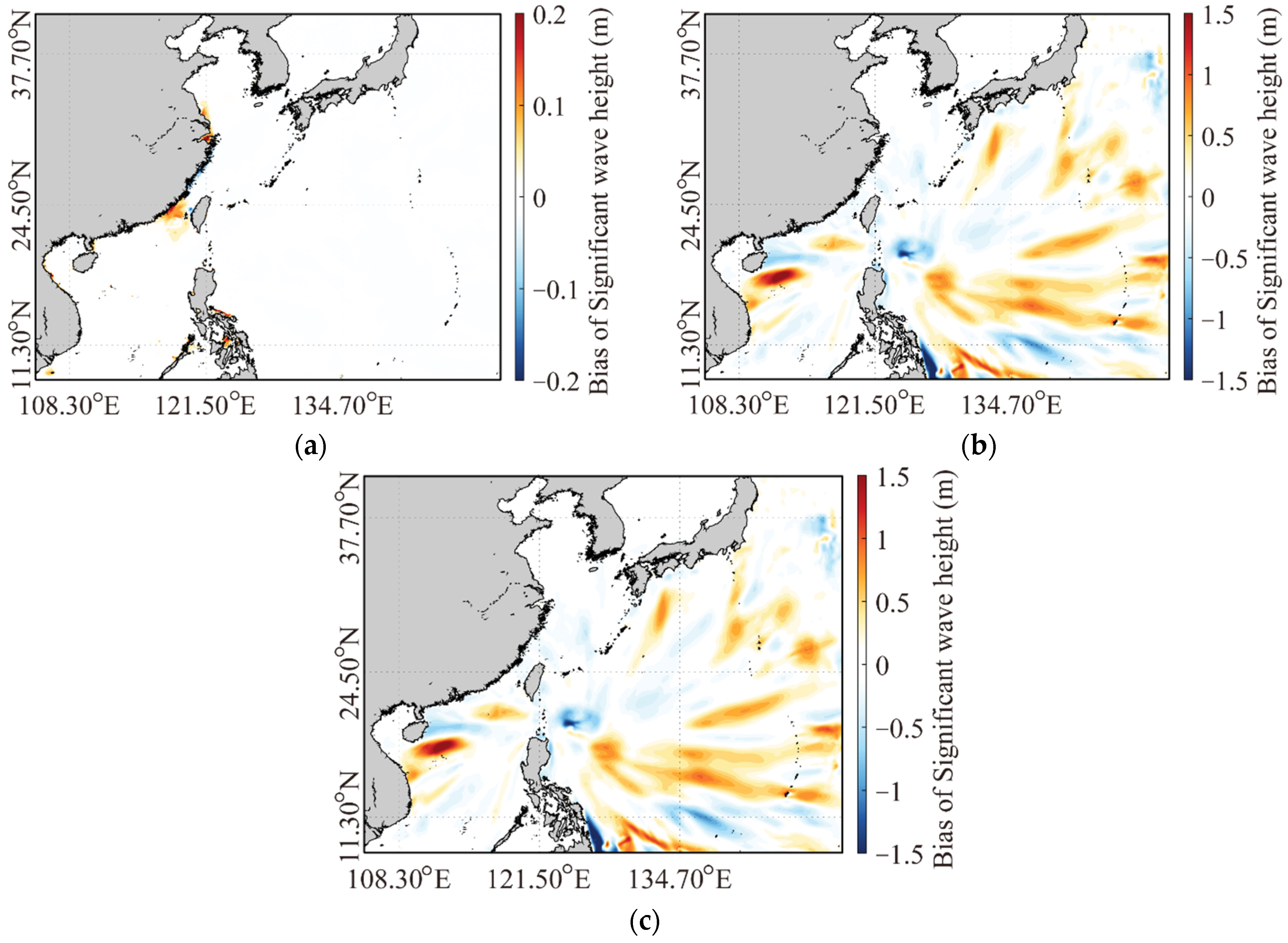
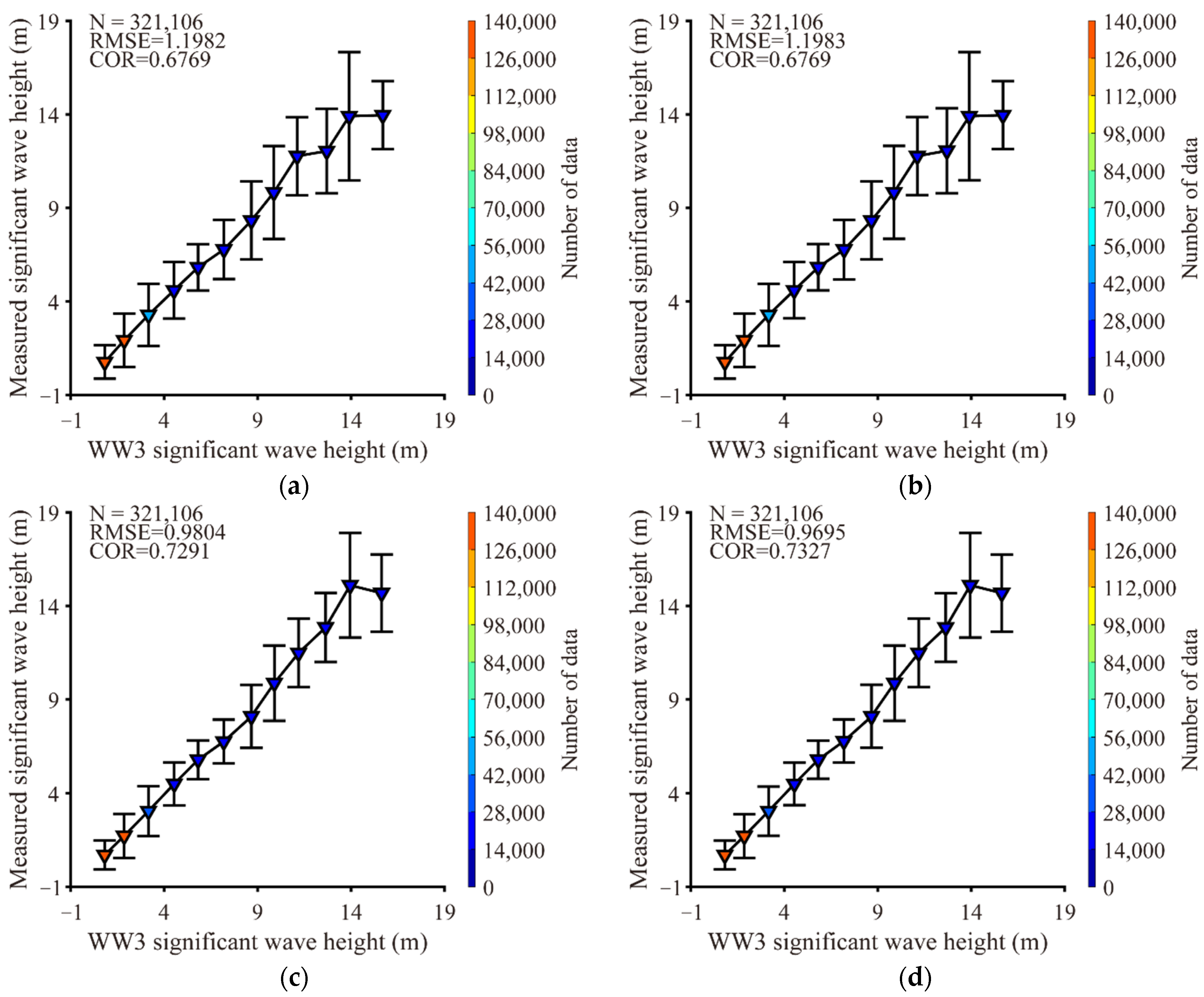
4.2. Influence of Current and Sea Level on Waves

Wind forcing at the ocean surface serves as the main energy source driving wave development. Moreover, ocean currents and sea level variations play crucial roles in influencing wave properties by altering surface roughness, particularly during TCs [147,148,149,150]. Currents modify the effective wind speed relative to the wave motion, thereby impacting the energy input into waves [151,152]. In areas with intense currents—such as flows generated by TCs, the Gulf Stream, or the Kuroshio—their influence is pronounced because strong horizontal gradients significantly affect surface wave patterns and air–sea exchanges [153,154]. Additionally, currents cause wave refraction and Doppler shifting, which results in wave fronts realigning in the direction of the current [26,155]. When currents run parallel to wave propagation, the wave spectrum undergoes changes: longer waves decrease in magnitude, the spectral peak moves toward higher frequencies, and directional spreading broadens [156,157]. The wave–current interaction involves momentum transfer via radiation stress from breaking waves [158,159], as well as vortex force mechanisms [160,161]. Currents also amplify the bottom friction acting on waves and intensify the frictional drag on currents when waves are present [159]. Recent investigations have assessed the performance of wave models incorporating wave–current coupling during TC events [137,162,163,164,165,166,167]. For example, Fan et al. [162] reported enhanced SWH predictions by WW3 for slow-moving cyclones, although the dominant wavelengths were still underestimated and wave direction effects were negligible. Moon et al. [137] and Chen et al. [163] improved model precision by integrating wave–current interaction with drag parameterization and dual-spectrum wave representations (mature and short waves). Lee et al. [73] evaluated a parameterization accounting for wave-induced dissipation stress, explicitly including the impact of breaking waves on currents across both deep and shallow water environments. Employing a coupled wave–circulation framework, Wang and Sheng [168] analyzed three extreme cases over the eastern Canadian shelf, discovering that SWH decreased by about 11% on the storm’s right flank but increased by roughly 5% on its left side due to asymmetrical wave–current interaction. Xu et al. [81] demonstrated that incorporating relative wind feedback through Stokes drift improved the wave field accuracy during Hurricane Juan.

Since the last century, global sea levels have shown a consistent rising trend [169,170,171,172], with projections indicating an accelerated increase throughout the upcoming century [173]. This sea level rise threatens coastal ecosystems by potentially causing degradation and altering both hydrodynamic regimes and hydrological conditions [174,175]. Furthermore, recent studies have identified a nonlinear relationship between elevated sea levels and changes in wave heights [176,177]. In regions along the coast regularly affected by TCs, wave heights tend to increase markedly once the sea level rise exceeds approximately one meter [178]. Using the FVCOM-SWAVE coupled modeling framework, Wu et al. [179] explored coastal ocean responses to TCs. Their results highlighted significant spatial and temporal variability in how wave–current interactions impact storm surge, with more pronounced effects observed on continental shelves compared to enclosed bay areas. Additionally, Wu et al. [179] showed that hurricane-induced wave–current interactions generate strong vertical shear in stratified water columns, which enhances offshore transport near the seabed and intensifies vertical mixing processes across the shelf zone. Hu et al. [150] and Yang et al. [180] investigated the effects of sea level changes and currents on wave modeling, observing that higher sea levels combined with reduced wave breaking and friction substantially influence SWH along coastal regions. Wang and Sheng [168] found clear asymmetry in SWH patterns when adding current forcing, causing decreases on the storm’s right side and increases on the left. This study reaffirmed the findings of Hu et al. [150] and Yang et al. [180] using wave fields from 20 TC events (listed in Table 1) in the WW3 wave model (Figure 11), corresponding well with their results, as shown in Figure 12 and Figure 13 and

Table 5. Comparison between SWH produced by WW3 and observations by altimeters (HY-2B and Jason2) and NDBC buoy.

	Case 1	Case 2	Case 3	Case 4
RMSE	1.1982	1.1983	0.9804	0.9695
Cor	0.6769	0.6769	0.7291	0.7327

Case 1: WW3-simulated SWH without water-level and current forcing. Case 2: WW3-simulated SWH with water level forcing. Case 3: WW3-simulated SWH with current forcing. Case 4: WW3-simulated SWH with water level and current forcing.

.

In a word, the current could influence the TC intensity and SWH structure of the TC, while sea level influences wave in the coastal area, which is important for the coastal protection and conservation strategies, especially under climate change. In future work, it is urgent to assess the ocean current evolution in the changing climate.

5. Effect of Wave on Water Temperature

Previous research indicates that four wave-induced forcings by breaking waves, nonbreaking waves, radiation stress, and Stokes drift play key roles in modulating heat and energy exchange at the ocean–atmosphere boundary, thereby impacting water temperature. The calculation methods for these processes are outlined in Appendix A. In this study, these four wave-driven mechanisms are evaluated using WW3 hindcasting outputs and then incorporated into sbPOM to simulate the temporal evolution of water temperature throughout the progression of 20 TCs.

Under the conditions of extreme wind speeds, breaking waves and whitecaps intensify ocean–atmosphere heat exchange by injecting substantial amounts of sea spray into the air. Spray droplets affect the ocean surface temperature and salinity by effectively increasing the air–sea interface area. The effect of spray on near-surface temperatures varies with its concentration [181]: moderate amounts of spray induce warming near the cyclone core and cooling farther away, whereas heavy spray intensifies warming compared to moderate levels. Consequently, spray influences both sensible and latent heat fluxes [182]. Large Eddy Simulation (LES) studies highlight the critical role of surface waves, particularly stochastic breaking waves, in upper ocean boundary layer dynamics [183,184,185,186]. Breaking waves inject turbulence and transfer wind momentum downward, which are incorporated into closure schemes of ocean circulation and mixing models [184,185,186]. Nonetheless, their overall contribution to ocean mixing is typically moderate [186,187]. In contrast, turbulence induced by non-breaking wave stirring significantly affects TC intensity [188], promoting mixing down to a depth of approximately 100 m [189,190]. The orbital motion generated by non-breaking waves causes vertical turbulence over depth scales much greater than the wave height [189], and in shallow waters, this turbulence can extend to the seabed after a TC event. Qiao et al. [191] introduced a parameterization of orbital motion-induced turbulence using a novel viscosity term, Bv, which was implemented in a 3D POM. Aijaz et al. [192] developed an updated parameterization for non-breaking waves, demonstrating its effectiveness in producing notable SST cooling and the deepening of the mixed layer. Building on Mellor’s foundational work [159,193,194], Xie et al. [168], developed a wave–current coupling framework that includes two- and three-dimensional radiation stresses scaled by depth, along with shear stresses, while resolving wetting–drying processes. Their results show that incorporating three-dimensional radiation stress substantially modifies wave characteristics and surge behavior. Langmuir turbulence, driven by Stokes drift through the Craik–Leibovich vortex mechanism arising from the interaction between Stokes drift and Eulerian vorticity, plays an important role [195,196]. During TC events, the wave induced turbulence evolves with the wind–wave field, therefore, turbulence closure schemes are needed to explicitly account for Langmuir effects. Yu et al. [197] incorporated Stokes-drift-enhanced mixing into the Mellor–Yamada 2.5 turbulence closure, resulting in a deeper mixed layer and improved vertical temperature profiles. Reichl et al. [198] further refined the K-profile first-moment closure by including Langmuir-driven turbulence, significantly improving predictions of upper-ocean temperature and currents during TCs.

Sun et al. [199,200] identified Stokes drift and nonbreaking wave contributions as critical factors in SST reduction during TCs. The present study further emphasizes the significant influence of these two mechanisms across 20 TC cases, where SST validation against Argo data produced COR values up to 0.9800 and RMSE around 1.79 m (refer to Figure 14 and

Table 6. Statistical assessment of the predicted sea surface temperatures (SSTs) by sbPOM with four individual wave forcings and their sum in comparison with Argo measurements.

	Wave Breaking	Nonbreaking Wave	Radiation Stress	Stokes Drift	All
RMSE (°C)	1.9687	1.7859	1.7864	1.7937	1.3909
Cor	0.9752	0.9802	0.9802	0.9800	0.9881

). Furthermore, including all four wave forcings can deepen the vertical mixing to nearly 100 m [199,200]. Our recent work evaluates how incorporating the four wave forcings, derived from WW3 model outputs, enhances temperature simulations within sbPOM [199,200]. Under TC conditions, SST showed a marked improvement, with the RMSE reaching 1.3909 m and a COR of 0.9881, as validated by Argo buoy observations (see Figure 15 and Table 6).

Significant gaps persist in understanding how four key wave effects, i.e., wave breaking, non-wave breaking, radiation stress and Stokes drift, impact ocean temperature simulation under extreme sea states. The synergistic roles of multiple wave effects (e.g., Stokes drift interacting with turbulent mixing) remain unquantified, especially during nonlinear amplification in TCs. High-resolution modeling is hindered by the lack of understanding of micro-scale processes (e.g., wave-induced convection) and non-universal parameterizations. Furthermore, cross-scale model coupling fails to bridge high-frequency wave forcing with longer-term thermal responses.

6. Conclusions and Outlook

It is well recognized that TCs under extreme conditions threaten lives and inflict considerable damage on both offshore and nearshore infrastructure. Consequently, this study evaluates the effectiveness of various parameterization of nonlinear wave–wave interaction schemes and C_d models, together with input forcing factors like surface currents and water levels in wave simulations across 20 TCs. The SWHs generated by WW3 and SWAN were validated using altimeter measurements from HY-2B and Jason2 satellites, along with in situ buoy data from NDBC. Furthermore, the impact of waves on SST cooling was examined by integrating four wave forcings by breaking waves, nonbreaking waves, radiation stress, and Stokes drift from WW3 into sbPOM. The key results are outlined as follows:

(1)

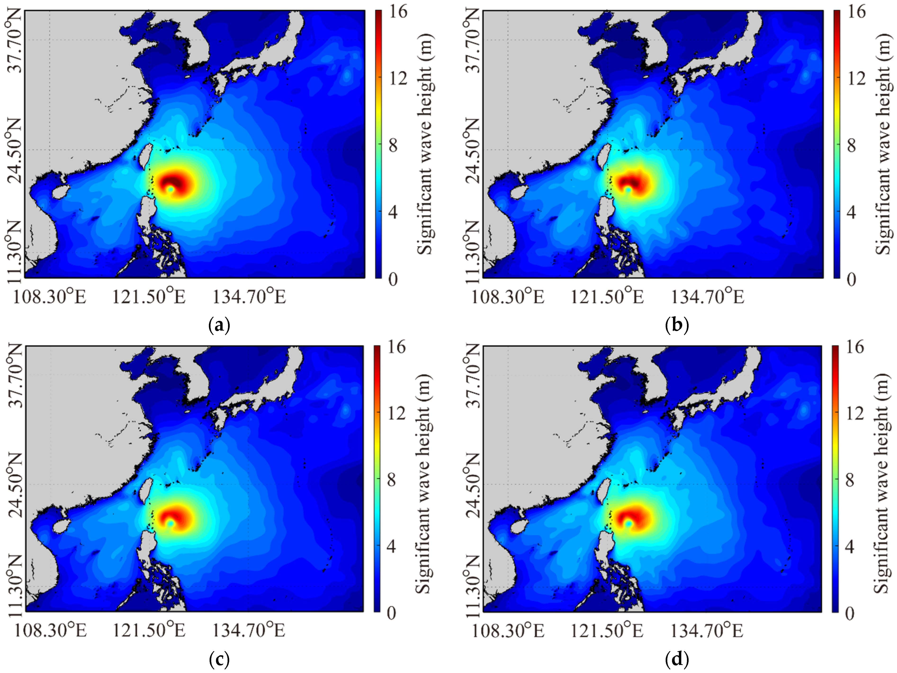
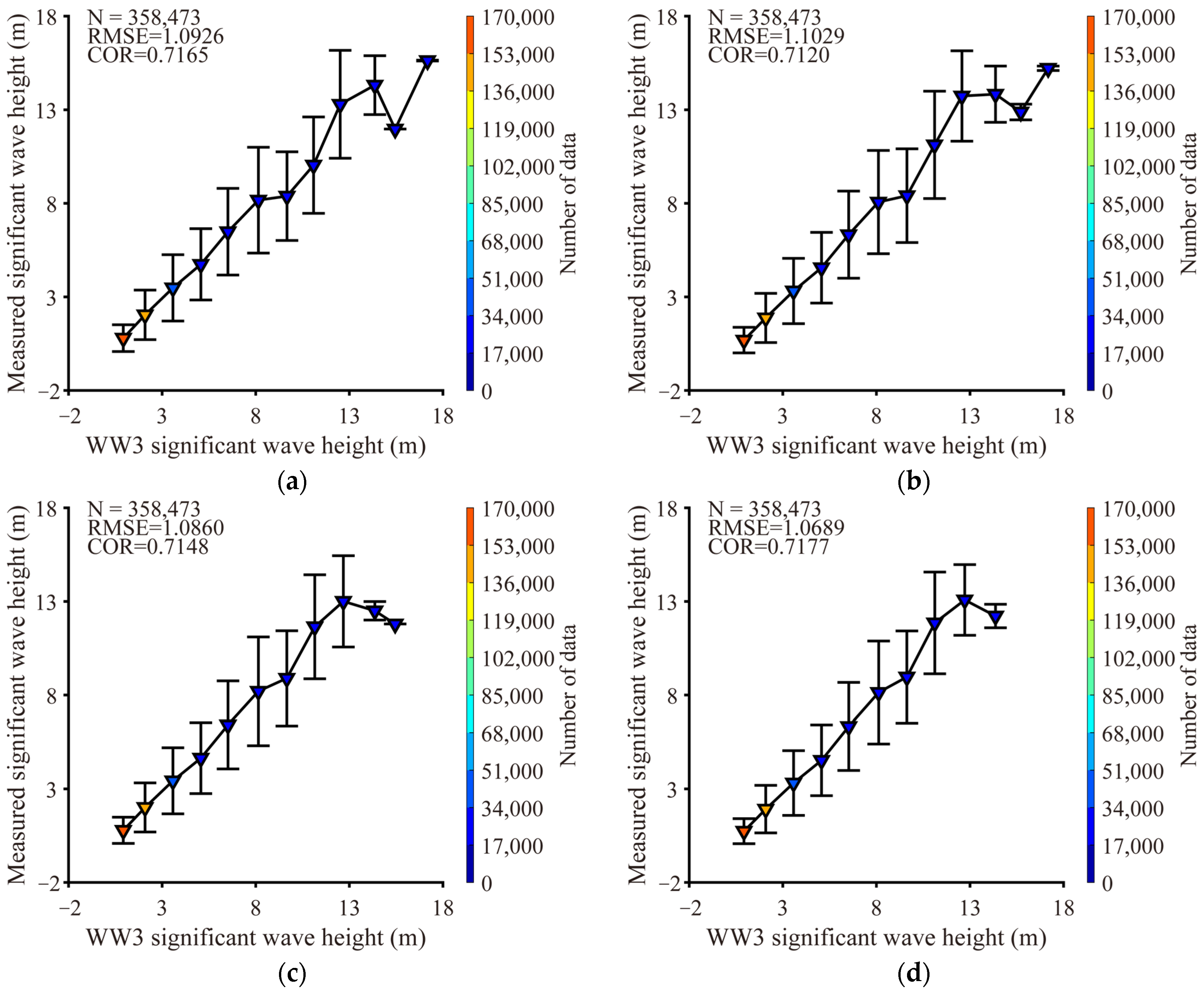
Nonlinear interactions between waves play a vital role in achieving precise high-resolution wave modeling during TCs. Four nonlinear interaction schemes, Generalized Multiple Discrete Interaction Approximation (GMD) Discrete Interaction Approximation (DIA) and the computationally expensive Wave-Ray Tracing (WRT), within WW3 were assessed in simulating SWH across 20 TC cases. It was found that the GMD2 provides a superior performance compared to DIA and WRT. Therefore, GMD2 is more suitable for environments with complex bathymetry and shallow water conditions.

(2)

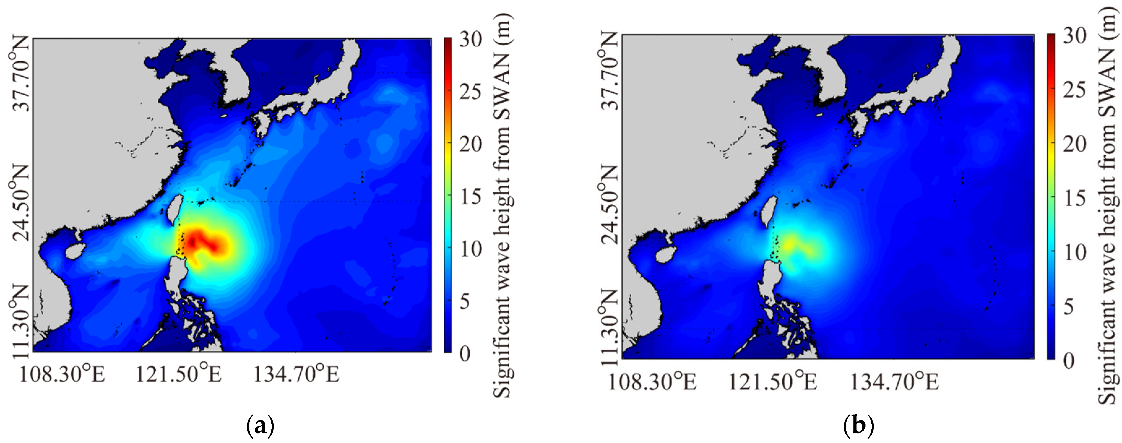
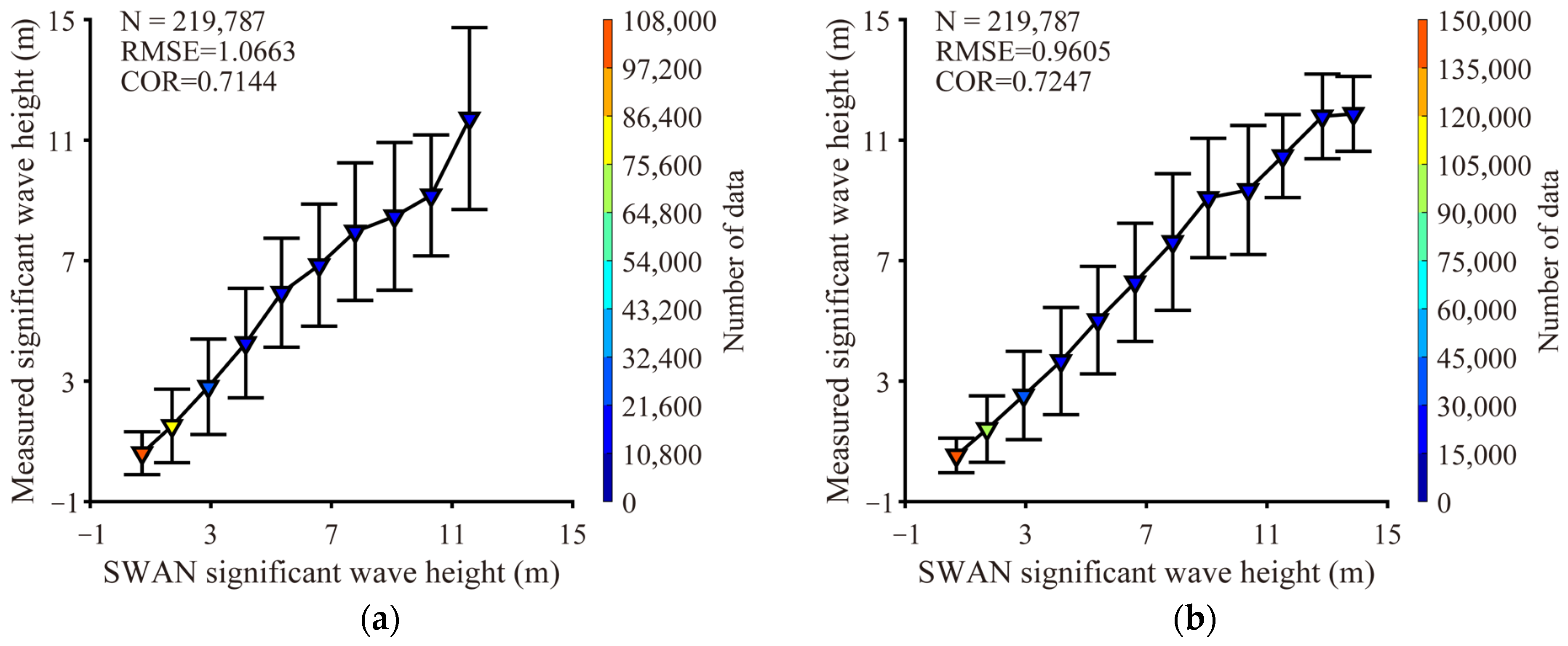
Conventional C_d schemes within WW3, including ST1 through ST6, tend to overpredict the wind drag at wind speeds exceeding 30 m/s, which leads to inflated wave growth and introduces notable biases in SWH. Recent developments have sought to overcome these shortcomings by implementing sea-state-dependent and wave boundary layer model (WBLM)-based parameterizations that dynamically incorporate factors such as wave age, spectral characteristics, and atmospheric stability. Among these advancements, a novel high-order C_d formulation derived from remote sensing observations was introduced and integrated into both WW3 and SWAN here. Within WW3, the updated ST6 scheme employing this C_d adjustment demonstrated superior accuracy over 20 TCs, lowering the RMSE to 0.7615 m and bias to −0.2552 m. Within SWAN, The updated ST6 scheme surpassed the default parameterization by achieving a correlation coefficient (COR) of 0.7647. These findings underscore the importance of adopting sophisticated, nonlinear Cd parameterizations specifically designed for cyclone environments, particularly under strong sea state–atmosphere feedback conditions. The ongoing refinement of C_d schemes is expected to improve the reliability of operational wave forecasts during extreme weather events.

(3)

Ocean currents influence relative wind speed, bend wave propagation paths, and redistribute wave energy, particularly in strong current regions with flows induced by TCs or the Kuroshio. These processes cause shifts in wave direction, changes the energy in long waves, and broaden the spectral distribution depending on the current direction relative to wave direction. The results from wave-current coupled modeling demonstrate that currents tend to lower SWH on the storm’s right side while increasing it on the left flank. Additionally, sea level rise—especially when exceeding one meter—intensifies coastal wave heights and alters nearshore hydrodynamics. Simulations conducted under different scenarios, including the presence or absence of currents and sea level variations, confirm these impacts. Therefore, accurately predicting SWH in shelf areas requires accounting for both wave–current interactions and sea level fluctuations. The incorporation of refined parameterizations, such as those representing Stokes drift and wave-induced radiation stresses, further improves the model performances during severe weather conditions.

(4)

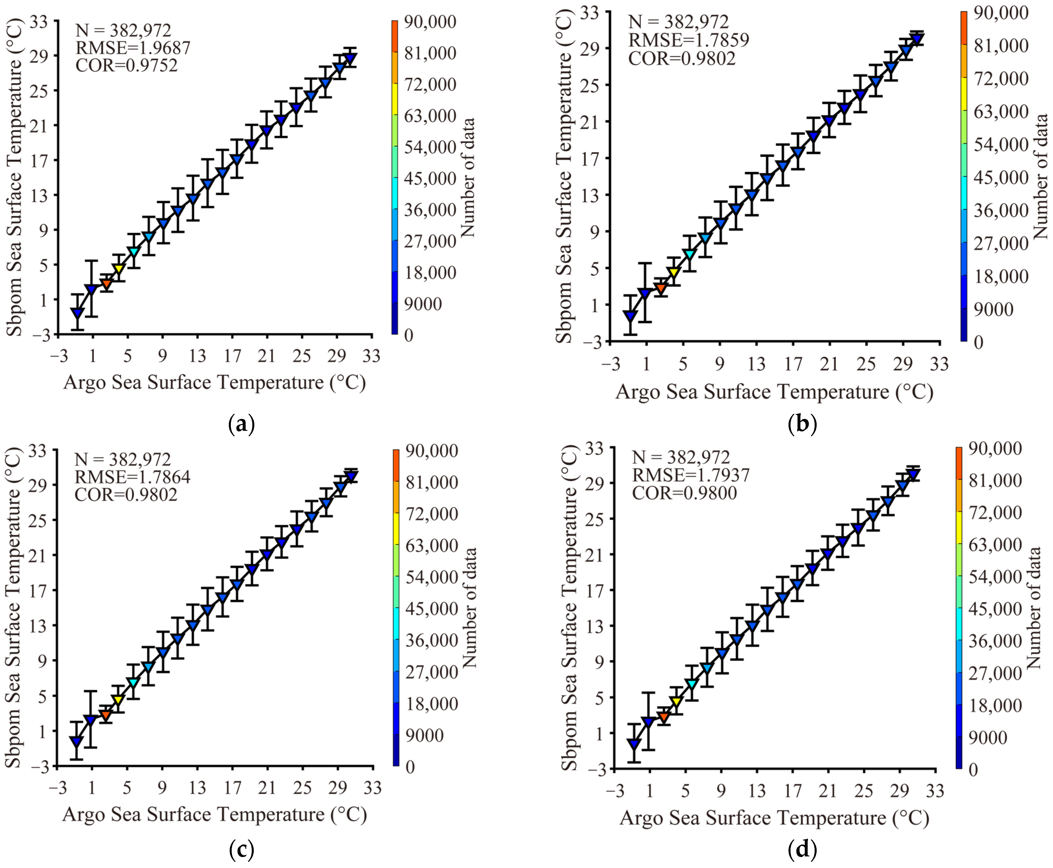
Wave-induced forcings through breaking and nonbreaking waves, radiation stress, and Stokes drift, are fundamental to regulating air–sea exchanges of heat and momentum during TCs. These forcings, simulated by WW3, are integrated into sbPOM to enhance the representation of sea surface temperature (SST). It was found that heat transfer is affected by breaking waves and sea spray, whereas nonbreaking waves play a vital role in intensifying mixing within the upper ocean. Radiation stress influences storm surge behavior and wave–current coupling, while Stokes drift drives Langmuir circulation, contributing to deeper mixed layers. Recent incorporations of these wave forcings into ocean circulation frameworks have yielded substantial improvements in SST forecasts during TCs, with RMSE declining to approximately 1.39 m and the correlation reaching 0.9881. Importantly, when these combined wave effects are considered, vertical mixing can extend to around 100 m, leading to more precise depictions of thermal stratification under cyclone-forced conditions.

Future studies should prioritize the integration among wave, ocean, and atmospheric models under TC scenarios, with particular emphasis on refining the parameterizations of wave–current interactions and sea-state-influenced air–sea fluxes as well as considerations of horizontal and vertical current shear [201]. Ongoing efforts will aim to further optimize C_d formulations and nonlinear interaction modules, enhance predictions by incorporating high-resolution observational datasets and apply machine learning methods to model tuning processes.

References

1. Ranson, M.; Kousky, C.; Ruth, M.; Jantarasami, L.; Crimmins, A.; Tarquiniom, L. Tropical and extratropical cyclone damages under climate change. Clim. Change 2014, 127, 227–241. [Google Scholar] [CrossRef]
2. Wang, H.J.; Sun, J.Q.; Fan, K. Relationships between the North Pacific Oscillation and the typhoon/hurricane frequencies. Sci. China Ser. D 2007, 50, 1409–1416. [Google Scholar] [CrossRef]
3. Mendelsohn, R.; Emanuel, K.; Chonabayashi, S.; Bakkensen, L. The impact of climate change on global tropical cyclone damage. Nat. Clim. Change 2012, 2, 205–209. [Google Scholar] [CrossRef]
4. Zhao, X.B.; Shao, W.Z.; Hao, M.Y.; Jiang, X.W. Novel approach to wind retrieval from Sentinel-1 SAR in tropical cyclones. Can. J. Remote Sens. 2023, 49, 2254839. [Google Scholar] [CrossRef]
5. Siegenthaler, T.D.T. Immediate impacts of a severe tropical cyclone on the microclimate of a rain-forest canopy in north-east Australia. J. Trop. Ecol. 2004, 20, 583–586. [Google Scholar]
6. Hoque, A.A.; Phinn, S.; Roelfsema, C.; Childs, I. Tropical cyclone disaster management using remote sensing and spatial analysis: A review. Int. J. Disast. Risk Reduct. 2017, 22, 345–354. [Google Scholar] [CrossRef]
7. Sampson, C.R.; Wittmann, P.A.; Serra, E.A.; Tolman, H.L.; Schauer, J.; Marchok, T. Evaluation of wave forecasts consistent with tropical cyclone warning center wind forecasts. Wea. Forecast. 2012, 28, 287–294. [Google Scholar] [CrossRef]
8. Jia, L.; Wu, S.; Han, B.; Cai, S.; Wu, R. Wave hindcast under tropical cyclone conditions in the south china sea: Sensitivity to wind fields. Acta Oceanol. Sin. 2023, 42, 36–53. [Google Scholar] [CrossRef]
9. Krogstad, H.E.; Barstow, S.F.; Aasen, S.E. Some recent developments in wave buoy measurement technology. Coast. Eng. 1999, 37, 309–329. [Google Scholar] [CrossRef]
10. Ananth, P.N.; Tatavarti, R.V.S.N.; Swain, J.; Rao, C.V.K.P. Observations of sea and swell using directional wave buoy. Proc. Indian Acad. Sci. Earth Planet. Sci. 1993, 102, 351–366. [Google Scholar] [CrossRef]
11. Nappo, C.J.; Chun, H.Y.; Lee, H.J. A parameterization of wave stress in the planetary boundary layer for use in mesoscale models. Atmos. Environ. 2004, 38, 2665–2675. [Google Scholar] [CrossRef]
12. Ye, X.M.; Liu, J.Q.; Lin, M.S.; Ding, J.; Zou, B.; Song, Q.J. Sea surface temperatures derived from COCTS onboard the HY-1C satellite. IEEE J. Sel. Top. Appl. Earth Obs. Remote Sens. 2021, 14, 1038–1047. [Google Scholar] [CrossRef]
13. Shao, W.Z.; Zhao, C.; Jiang, X.W.; Sun, Z.F.; Wang, X.Q.; Wang, J.; Cai, L.N. Characteristics of suspended sediment in Sentinel-1 synthetic aperture radar observations. Remote Sens. Lett. 2021, 12, 1167–1179. [Google Scholar] [CrossRef]
14. Wang, X.; Bai, X.; Zhang, M.; Wu, C. High-Resolution seawater salinity sensor based on temperature self-compensating optical interferometer. IEEE Sens. J. 2024, 24, 1374–1382. [Google Scholar] [CrossRef]
15. Stoffelen, A.; Anderson, D. Scatterometer data interpretation: Estimation and validation of the transfer function CMOD4. J. Geophys. Res. Oceans 1997, 102, 5767–5780. [Google Scholar] [CrossRef]
16. Quilfen, Y.; Chapron, B.; Elfouhaily, T.; Katsaros, K.; Tournadre, J. Observation of tropical cyclones by high-resolution scatterometry. J. Geophys. Res. Oceans 1998, 103, 7767–7786. [Google Scholar] [CrossRef]
17. Shao, W.Z.; Jiang, T.; Jiang, X.W.; Zhang, Y.G.; Zhou, W. Evaluation of sea surface winds and waves retrieved from the Chinese HY-2B data. IEEE J. Sel. Top. Appl. Earth Obs. Remote. Sens. 2021, 14, 9624–9635. [Google Scholar] [CrossRef]
18. Chen, J.L.; Hao, M.Y.; Shao, W.Z.; Marino, A.; Hu, Y.Y.; Song, X.G. Validation of wind speed retrieval from HY-2B calibration microwave radiometer data during tropical cyclones. Remote Sens. Lett. 2024, 15, 700–708. [Google Scholar] [CrossRef]
19. Shao, W.Z.; Zhou, Y.H.; Hu, Y.Y.; Li, Y.; Zhou, Y.S.; Zhang, Q.J. Range current retrieval fromsentinel-1 SAR ocean product based on deep learning. Remote Sens. Lett. 2024, 15, 145–156. [Google Scholar] [CrossRef]
20. Hauser, D.; Tison, C.; Amiot, T.; Delaye, L.; Corcoral, N.; Castillan, P. SWIM: The first spaceborne wave scatterometer. IEEE Trans. Geosci. Remote Sens. 2017, 55, 3000–3014. [Google Scholar] [CrossRef]
21. Hao, M.; Hu, Y.; Shao, W.; Migliaccio, M.; Jiang, X.; Wang, Z. Advance in sea surface wind and wave retrieval from synthetic aperture radar image: An Overview. J. Ocean Univ. 2025, 24, 821–839. [Google Scholar] [CrossRef]
22. Zhou, Y.H.; Shao, W.Z.; Wei, M.; Jiang, X.W.; Li, Y. Preliminary analysis of calibration for Chinese civilian 1mC-SAR. Remote Sens. Lett. 2024, 15, 709–718. [Google Scholar] [CrossRef]
23. Zhou, Y.H.; Hao, M.Y.; Shao, W.Z.; Marino, A.; Song, X.G.; Jiang, X.W. Preliminary analysis of wind and wave retrieval from Chinese 1mC-SAR image. Eur. J. Remote Sens. 2024, 57, 2364706. [Google Scholar] [CrossRef]
24. Jiang, T.; Shao, W.Z.; Hu, Y.Y.; Zheng, G.; Shen, W. L-band analysis of the effects of oil slicks on sea wave characteristics. J. Ocean Univ. China 2023, 22, 9–20. [Google Scholar] [CrossRef]
25. The WAMDI Group. The WAM model-A third generation ocean wave prediction model. J. Phys. Oceanogr. 1998, 18, 1775–1810. [Google Scholar]
26. Tolman, L. A third-generation model for wind waves on slowly varying, unsteady, and inhomogeneous depths and currents. J. Phys. Oceanogr. 1991, 21, 782–797. [Google Scholar] [CrossRef]
27. Holthuijsen, L. The Continued Development of the Third-Generation Shallow Water Wave Model ‘SWAN’; TU Delft Department of Hydraulic Engineering: Delft, The Netherlands, 2001; Volume 32, pp. 185–186. [Google Scholar]
28. Xie, D.; Zou, Q.; Cannon, J.W. Application of SWAN+ADCIRC to tide-surge and wave smulation in Gulf of Maine during Patriot’s Day Storm. Water Sci. Eng. 2016, 9, 33–41. [Google Scholar] [CrossRef]
29. Xie, D.; Zou, Q.P.; Mignone, A.; MacRae, J.D. Coastal flooding from wave overtopping and sea level rise adaptation in the Northeastern USA. Coast. Eng. 2019, 150, 39–58. [Google Scholar] [CrossRef]
30. Zou, Q.; Xie, D. Tide-Surge and wave interaction in the Gulf of Maine during an extratropical storm. Ocean Dyn. 2016, 66, 1715–1732. [Google Scholar] [CrossRef]
31. Liu, N.; Ling, T.J.; Wang, H.; Zhang, Y.F.; Gao, Z.Y.; Wang, Y. Numerical simulation of Typhoon Muifa (2011) using a Coupled Ocean-Atmosphere-Wave-Sediment Transport (COAWST) modeling system. J. Ocean Univ. China 2015, 14, 199–209. [Google Scholar] [CrossRef]
32. Nittis, K.; Perivoliotis, L.; Korres, G.; Tziavos, C.; Thanos, I. Operational monitoring and forecasting for marine environmental applications in the Aegean Sea. Environ. Model. Softw. 2006, 21, 243–257. [Google Scholar] [CrossRef]
33. Jordi, A.; Wang, D.P. Sbpom: A parallel implementation of Princenton ocean model. Environ. Model. Softw. 2012, 38, 59–61. [Google Scholar] [CrossRef]
34. Stepanov, V.N.; Haines, K. Mechanisms of Atlantic meridional overturning circulation variability simulated by the NEMO model. Ocean Sci. 2014, 10, 645–656. [Google Scholar] [CrossRef]
35. Yao, F.C.; Johns, W.E. A HYCOM modeling study of the Persian Gulf: 1. Model configurations and surface circulation. J. Geophys. Res. 2010, 115, C11017. [Google Scholar] [CrossRef]
36. Wei, H.; Hainbucher, D.; Pohlmann, T.; Feng, S.; Suendermann, J. Tidal-induced Lagrangian and Eulerian mean circulation in the Bohai sea. J. Mar. Syst. 2004, 44, 141–151. [Google Scholar] [CrossRef]
37. Sun, Z.; Shao, W.; Wang, W.; Zhou, W.; Yu, W.; Shen, W. Analysis of wave-induced Stokes transport effects on sea surface temperature simulations in the Western Pacific Ocean. J. Mar. Sci. Eng. 2021, 9, 834. [Google Scholar] [CrossRef]
38. Prasad, T.G.; Hogan, P.J. Upper-ocean response to Hurricane Ivan in a 1/25° nested Gulf of Mexico HYCOM. J. Geophys. Res. Oceans 2007, 112, C04013. [Google Scholar] [CrossRef]
39. Zamudio, L.; Hogan, P.J. Nesting the Gulf of Mexico in Atlantic HYCOM: Oceanographic processes generated by Hurricane Ivan. Ocean. Model. 2008, 21, 106–125. [Google Scholar] [CrossRef]
40. Chen, C.S.; Liu, H.; Beardsley, R.C. An unstructured, finite-volume, three-dimensional, primitive equation ocean model: Application to coastal ocean and estuaries. J. Atmos. Ocean. Technol. 2003, 20, 159–186. [Google Scholar] [CrossRef]
41. Wang, J.; Kuang, C.; Fan, D.; Xing, W.; Qin, R.; Zou, Q. Spatio-Temporal variation in suspended sediment during Typhoon Ampil under wave-current interactions in the Yangtze River Estuary. Water 2024, 16, 1783. [Google Scholar] [CrossRef]
42. Rezende, L.F.; Silva, P.A.; Cirano, M.; Peliz, Á.; Dubert, J. Mean circulation, seasonal cycle, and eddy interactions in the eastern Brazilian margin, a nested ROMS model. J. Coast. Res. 2011, 27, 329–347. [Google Scholar] [CrossRef]
43. Marshall, J.; Hill, C.; Perelman, L.; Adcroft, A. Hydrostatic, quasi-hydrostatic, and nonhydrostatic ocean modeling. J. Geophys. Res. Oceans 1997, 102, 5733–5752. [Google Scholar] [CrossRef]
44. Fringer, O.B.; Gerritsen, M.; Street, R.L. An unstructured-grid, finite-volume, nonhydrostatic, parallel coastal ocean simulator. Ocean. Model. 2006, 14, 139–173. [Google Scholar] [CrossRef]
45. Huang, H.; Song, P.Y.; Qiu, S.; Guo, Q.Y.; Chen, X.E. A nonhydrostatic oceanic regional model, ORCTM v1, for internal solitary wave simulation. Geosci. Model Dev. 2023, 16, 109–133. [Google Scholar] [CrossRef]
46. Wu, Z.Y.; Jiang, C.B.; Deng, B.; Chen, J.; Cao, Y.G.; Li, L.J. Evaluation of numerical wave model for typhoon wave simulation in South China Sea. Water Sci. Eng. 2018, 11, 229–235. [Google Scholar] [CrossRef]
47. Kong, C.Y.; Cao, H.S.; Pan, X.S.; Zhang, W.Y. Numerical simulation of typhoon waves along the offshore China Seas. Appl. Mech. Mater. 2013, 303–306, 2736–2739. [Google Scholar] [CrossRef]
48. Wang, J.C.; Zhang, J.; Yang, J.G. Numerical simulation and preliminary analysis on ocean waves during typhoon nesat in south china sea and adjacent areas. Chin. J. Ocean. Limnol. 2014, 32, 665–680. [Google Scholar] [CrossRef]
49. Sun, Y.; Wang, K.; Zhong, X.; Zhou, Z.; Zhang, J. Assess the typhoon-driven extreme wave conditions in Manila bay through numerical simulation and statistical analysis. Appl. Ocean Res. 2021, 109, 102565. [Google Scholar] [CrossRef]
50. Sheng, Y.P.; Zhang, Y.; Paramygin, V.A. Simulation of storm surge, wave, and coastal inundation in the northeastern Gulf of Mexico region during Hurricane Ivan in 2004. Ocean. Model. 2010, 35, 314–331. [Google Scholar] [CrossRef]
51. Huang, Y.; Weisberg, R.H.; Zheng, L.; Zijlema, M. Gulf of Mexico hurricane wave simulations using swan: Bulk formula-based drag coefficient sensitivity for Hurricane Ike. J. Geophys. Res. Oceans 2013, 118, 3916–3938. [Google Scholar] [CrossRef]
52. Bhaskaran, P.K.; Nayak, S.; Bonthu, S.R.; Murty, P.L.N.; Sen, D. Performance and validation of a coupled parallel ADCIRC–SWAN model for THANE cyclone in the Bay of Bengal. Environ. Fluid Mech. 2013, 13, 601–623. [Google Scholar] [CrossRef]
53. Emanuel, K.; Solomon, S.; Folini, D.; Davis, S.; Cagnazzo, C. Influence of Tropical Tropopause Layer Cooling on Atlantic Hurricane Activity. J. Clim. 2013, 26, 2288–2301. [Google Scholar] [CrossRef]
54. Emanuel, K. Contribution of Tropical Cyclones to Meridional Heat Transport by the Oceans. J. Geophys. Res.-Atmos. 2001, 106, 14771–14781. [Google Scholar] [CrossRef]
55. Bruneau, N.; Toumi, R.; Wang, S. Impact of Wave Whitecapping on Land Falling Tropical Cyclones. Sci. Rep. 2018, 8, 652. [Google Scholar] [CrossRef]
56. Stoney, L.; Walsh, K.; Babanin, A.V.; Ghantous, M.; Govekar, P.; Young, I. Simulated Ocean Response to Tropical Cyclones: The Effect of a Novel Parameterization of Mixing from Unbroken Surface Waves. J. Adv. Model. Earth Syst. 2017, 9, 759–780. [Google Scholar] [CrossRef]
57. Le Traon, P.Y.; Reppucci, A.; Alvarez Fanjul, E.; Aouf, L.; Behrens, A.; Belmonte, M.; Bentamy, A.; Bertino, L.; Brando, V.E.; Kreiner, M.B.; et al. From Observation to Information and Users: The Copernicus Marine Service Perspective. Front. Mar. Sci. 2019, 6, 234. [Google Scholar] [CrossRef]
58. Pisano, A.; Marullo, S.; Artale, V.; Falcini, F.; Yang, C.; Leonelli, F.E.; Santoleri, R.; Nardelli, B.B. New Evidence of Mediterranean Climate Change and Variability from Sea Surface Temperature Observations. Remote Sens. 2020, 12, 132. [Google Scholar] [CrossRef]
59. Mason, E.; Ruiz, S.; Bourdalle-Badie, R.; Reffray, G.; Garcia-Sotillo, M.; Pascual, A. New Insight into 3-D Mesoscale Eddy Properties from CMEMS Operational Models in the Western Mediterranean. Ocean Sci. 2019, 15, 1111–1131. [Google Scholar] [CrossRef]
60. Schenkel, B.A.; Hart, R.E. An Examination of Tropical Cyclone Position, Intensity, and Intensity Life Cycle within Atmospheric Reanalysis Datasets. J. Clim. 2012, 25, 3453–3475. [Google Scholar] [CrossRef]
61. Li, X.; Yang, J.; Han, G.; Ren, L.; Zheng, G.; Chen, P.; Zhang, H. Tropical Cyclone Wind Field Reconstruction and Validation Using Measurements from SFMR and SMAP Radiometer. Remote Sens. 2022, 14, 3929. [Google Scholar] [CrossRef]
62. Carton, J.A.; Giese, B.S. A Reanalysis of Ocean Climate Using Simple Ocean Data Assimilation (SODA). Mon. Weather Rev. 2008, 136, 2999–3017. [Google Scholar] [CrossRef]
63. Kanamitsu, M.; Ebisuzaki, W.; Woollen, J.; Yang, S.K.; Hnilo, J.J.; Fiorino, M.; Potter, G.L. NCEP-DOE AMIP-II Reanalysis (R-2). Bull. Am. Meteorol. Soc. 2002, 83, 1631–1643. [Google Scholar] [CrossRef]
64. Wong, A.P.S.; Wijffels, S.E.; Riser, S.C.; Pouliquen, S.; Hosoda, S.; Roemmich, D.; Gilson, J.; Johnson, G.C.; Martini, K.; Murphy, D.J.; et al. Argo Data 1999-2019: Two Million Temperature-Salinity Profiles and Subsurface Velocity Observations From a Global Array of Profiling Floats. Front. Mar. Sci. 2020, 7, 700. [Google Scholar] [CrossRef]
65. Guerin, C.-A.; Poisson, J.-C.; Piras, F.; Amarouche, L.; Lalaurie, J.-C. Ku-/Ka-Band Extrapolation of the Altimeter Cross Section and Assessment with Jason2/AltiKa Data. IEEE Trans. Geosci. Remote Sens. 2017, 55, 5679–5686. [Google Scholar] [CrossRef]
66. Mukhlas, N.A.; Zaki, N.I.M.; Abu Husain, M.K.; Ahmad, S.Z.A.S.; Najafian, G. Numerical Formulation Based on Ocean Wave Mechanics for Offshore Structure Analysis—A Review. Ships Offshore Struct. 2022, 17, 1731–1742. [Google Scholar] [CrossRef]
67. Chalikov, D.; Babanin, A.V. Comparison of Linear and Nonlinear Extreme Wave Statistics. Acta Oceanol. Sin. 2016, 35, 99–105. [Google Scholar] [CrossRef]
68. Chalikov, D. Freak Waves: Their Occurrence and Probability. Phys. Fluids 2009, 21, 076602. [Google Scholar] [CrossRef]
69. Crespo, A.J.C.; Gomez-Gesteira, M.; Carracedo, P.; Dalrymple, R.A. Hybridation of Generation Propagation Models and SPH Model to Study Severe Sea States in Galician Coast. J. Mar. Syst. 2008, 72, 135–144. [Google Scholar] [CrossRef]
70. Korres, G.; Papadopoulos, A.; Katsafados, P.; Ballas, D.; Perivoliotis, L.; Nittis, K. A 2-Year Intercomparison of the WAM-Cycle4 and the WAVEWATCH-III Wave Models Implemented within the Mediterranean Sea. Mediterr. Mar. Sci. 2011, 12, 129–152. [Google Scholar] [CrossRef]
71. Gaztelumendi, S.; Gonzalez, M.; Egana, J.; Rubio, A.; Gelpi, I.R.; Fontan, A.; Otxoa De Alda, K.; Ferrer, L.; Alchaarani, N.; Mader, J.; et al. Implementation of an Operational Oceano-Meteorological System for the Basque Country. Thalassas 2010, 26, 151–167. [Google Scholar]
72. Pianca, C.; Mazzini, P.L.F.; Siegle, E. Brazilian Offshore Wave Climate Based on Nww3 Reanalysis. Braz. J. Oceanogr. 2010, 58, 53–70. [Google Scholar] [CrossRef]
73. Lee, H.S.; Yamashita, T.; Hsu, J.R.-C.; Ding, F. Integrated Modeling of the Dynamic Meteorological and Sea Surface Conditions during the Passage of Typhoon Morakot. Dyn. Atmos. Oceans 2013, 59, 1–23. [Google Scholar] [CrossRef]
74. The WAVEWATCH-III Development Group. User Manual and System Documentation of WAVEWATCH III Version 5.16; Technical Note 329; National Oceanic and Atmospheric Administration: College Park, MD, USA, 2016; Volume 276, p. 326. [Google Scholar]
75. Booij, N.; Ris, R.C.; Holthuijsen, L.H. A Third-Generation Wave Model for Coastal Regions—1. Model Description and Validation. J. Geophys. Res.-Oceans 1999, 104, 7649–7666. [Google Scholar] [CrossRef]
76. Mulligan, R.P.; Perrie, W.; Toulany, B.; Smith, P.C.; Hay, A.E.; Bowen, A.J. Performance of Nowcast and Forecast Wave Models for Lunenburg Bay, Nova Scotia. Atmos.-Ocean 2011, 49, 1–7. [Google Scholar] [CrossRef]
77. Ou, S.H.; Liau, J.M.; Hsu, T.W.; Tzang, S.Y. Simulating Typhoon Waves by SWAN Wave Model in Coastal Waters of Taiwan. Ocean Eng. 2002, 29, 947–971. [Google Scholar] [CrossRef]
78. Bolanos-Sanchez, R.; Sanchez-Arcilla, A.; Cateura, J. Evaluation of Two Atmospheric Models for Wind-Wave Modelling in the NW Mediterranean. J. Mar. Syst. 2007, 65, 336–353. [Google Scholar] [CrossRef]
79. Rogers, W.E.; Kaihatu, J.M.; Petit, H.; Booij, N.; Holthuijsen, L.H. Diffusion Reduction in an Arbitrary Scale Third Generation Wind Wave Model. Ocean Eng. 2002, 29, 1357–1390. [Google Scholar] [CrossRef]
80. Signell, R.P.; Carniel, S.; Cavaleri, L.; Chiggiato, J.; Doyle, J.D.; Pullen, J.; Sclavo, M. Assessment of Wind Quality for Oceanographic Modelling in Semi-Enclosed Basins. J. Mar. Syst. 2005, 53, 217–233. [Google Scholar] [CrossRef]
81. Xu, F.; Perrie, W.; Toulany, B.; Smith, P.C. Wind-Generated Waves in Hurricane Juan. Ocean Model. 2007, 16, 188–205. [Google Scholar] [CrossRef]
82. Jin, K.R.; Ji, Z.G. Calibration and Verification of a Spectral Wind-Wave Model for Lake Okeechobee. Ocean Eng. 2001, 28, 571–584. [Google Scholar] [CrossRef]
83. Smagorinsky, J.; Manabe, S.; Holloway, J.L. Numerical Results from a Nine-Level General Circulation Model of the Atmosphere1. Mon. Weather. Rev. 1965, 93, 727–768. [Google Scholar] [CrossRef]
84. Nakanishi, M.; Niino, H. Development of an Improved Turbulence Closure Model for the Atmospheric Boundary Layer. J. Meteorol. Soc. Jpn. 2009, 87, 895–912. [Google Scholar] [CrossRef]
85. Chen, W.; Chen, J.; Shi, J. Regional Differences in the Effects of Various Stokes Drifts on the Cooling of the Marine Environment under Different Wave Conditions. Environ. Res. 2024, 255, 119191. [Google Scholar] [CrossRef]
86. Fang, S.-C. Research on a Numerical Simulation Model of Marine Drifting Debris: A Case Study of Penghu Waters. Ocean Sci. J. 2024, 59, 33. [Google Scholar] [CrossRef]
87. Chen, C.; Beardsley, R.C.; Cowles, G. An unstructured grid, finite-volume coastal ocean model (FVCOM) system. Oceanography 2006, 19, 78–89. [Google Scholar] [CrossRef]
88. Chen, C.; Huang, H.; Beardsley, R.C.; Liu, H.; Xu, Q.; Cowles, G. A Finite Volume Numerical Approach for Coastal Ocean Circulation Studies: Comparisons with Finite Difference Models. J. Geophys. Res.-Oceans 2007, 112, C03018. [Google Scholar] [CrossRef]
89. Huang, H.; Chen, C.; Blanton, J.O.; Andrade, F.A. A Numerical Study of Tidal Asymmetry in Okatee Creek, South Carolina. Estuar. Coast. Shelf Sci. 2008, 78, 190–202. [Google Scholar] [CrossRef]
90. Isobe, A.; Beardsley, R.C. An Estimate of the Cross-Frontal Transport at the Shelf Break of the East China Sea with the Finite Volume Coastal Ocean Model. J. Geophys. Res.-Oceans 2006, 111, C03012. [Google Scholar] [CrossRef]
91. Lin, S.; Sheng, J. Assessing the Performance of Wave Breaking Parameterizations in Shallow Waters in Spectral Wave Models. Ocean Model. 2017, 120, 41–59. [Google Scholar] [CrossRef]
92. Filipot, J.-F.; Ardhuin, F. A Unified Spectral Parameterization for Wave Breaking: From the Deep Ocean to the Surf Zone. J. Geophys. Res.-Oceans 2012, 117, C00J08. [Google Scholar] [CrossRef]
93. Kuznetsova, A.; Baydakov, G.; Dosaev, A.; Troitskaya, Y. Drag Coefficient Parameterization under Hurricane Wind Conditions. Water 2023, 15, 1830. [Google Scholar] [CrossRef]
94. Makin, V.K. A Note on a Parameterization of the Sea Drag. Bound.-Layer Meteor. 2003, 106, 593–600. [Google Scholar] [CrossRef]
95. Moon, I.-J.; Ginis, I.; Hara, T. Impact of the Reduced Drag Coefficient on Ocean Wave Modeling under Hurricane Conditions. Mon. Weather Rev. 2008, 136, 1217–1223. [Google Scholar] [CrossRef]
96. Lin, S.; Sheng, J. Revisiting Dependences of the Drag Coefficient at the Sea Surface on Wind Speed and Sea State. Cont. Shelf Res. 2020, 207, 104188. [Google Scholar] [CrossRef]
97. Lv, J.; Zhang, W.; Shi, J.; Wu, J.; Wang, H.; Cao, X.; Wang, Q.; Zhao, Z. The Wave Period Parameterization of Ocean Waves and Its Application to Ocean Wave Simulations. Remote Sens. 2023, 15, 5279. [Google Scholar] [CrossRef]
98. Mentaschi, L.; Perez, J.; Besio, G.; Mendez, F.J.; Menendez, M. Parameterization of Unresolved Obstacles in Wave Modelling: A Source Term Approach. Ocean Model. 2015, 96, 93–102. [Google Scholar] [CrossRef]
99. Kuznetsova, A.M.; Dosaev, A.S.; Baydakov, G.A.; Sergeev, D.A.; Troitskaya, Y.I. Adaptation of the Parameterization of the Nonlinear Energy Transfer for Short Fetch Conditions in the WAVEWATCH III Wave Prediction Model. Izv. Atmos. Ocean. Phys. 2020, 56, 191–199. [Google Scholar] [CrossRef]
100. Walsh, K.; Govekar, P.; Babanin, A.V.; Ghantous, M.; Spence, P.; Scoccimarro, E. The Effect on Simulated Ocean Climate of a Parameterization of Unbroken Wave-Induced Mixing Incorporated into the k-Epsilon Mixing Scheme. J. Adv. Model. Earth Syst. 2017, 9, 735–758. [Google Scholar] [CrossRef]
101. Ji, C.; Jiang, Q.; Ma, D.; Wu, Y.; Ran, G.; Kong, X.; Zhang, Q. Parameterization of Surface Roller Evolution in Wave-Induced Current Modeling. Ocean Model. 2025, 196, 102522. [Google Scholar] [CrossRef]
102. Ren, D.; Hua, F.; Yang, Y.; Sun, B. The Improved Model of Estimating Global Whitecap Coverage Based on Satellite Data. Acta Oceanol. Sin. 2016, 35, 66–72. [Google Scholar] [CrossRef]
103. Kim, T.; Moon, J.-H.; Kang, K. Uncertainty and Sensitivity of Wave-Induced Sea Surface Roughness Parameterisations for a Coupled Numerical Weather Prediction Model. Tellus Ser. A-Dyn. Meteorol. Oceanol. 2018, 70, 1445379. [Google Scholar] [CrossRef]
104. Montgomery, M.T.; Möller, J.D.; Nicklas, C.T. Linear and Nonlinear Vortex Motion in an Asymmetric Balance Shallow Water Model. J. Atmos. Sci. 1999, 56, 749–768. [Google Scholar] [CrossRef]
105. Young, I.R. Directional Spectra of Hurricane Wind Waves. J. Geophys. Res.-Oceans 2006, 111, C08020. [Google Scholar] [CrossRef]
106. Shao, W.; Sheng, Y.; Li, H.; Shi, J.; Ji, Q.; Tan, W.; Zuo, J. Analysis of Wave Distribution Simulated by WAVEWATCH-III Model in Typhoons Passing Beibu Gulf, China. Atmosphere 2018, 9, 265. [Google Scholar] [CrossRef]
107. Hu, Y.; Shao, W.; Wei, Y.; Zuo, J. Analysis of Typhoon-Induced Waves along Typhoon Tracks in the Western North Pacific Ocean, 1998–2017. J. Mar. Sci. Eng. 2020, 8, 521. [Google Scholar] [CrossRef]
108. Hasselmann, K. On the non-linear energy transfer in a gravity wave spectrum Part 1. General theory. J. Fluid Mech. 1962, 12, 481–500. [Google Scholar] [CrossRef]
109. Xu, Y.; He, H.; Song, J.; Hou, Y.; Li, F. Observations and Modeling of Typhoon Waves in the South China Sea. J. Phys. Oceanogr. 2017, 47, 1307–1324. [Google Scholar] [CrossRef]
110. Hasselmann, S.; Hasselmann, K.; Allender, J.H.; Barnett, T.P. Computations and parameterizations of the non-linear energy transfer in a gravity-wave spectrum, Part 2: Parameterizations of the non-linear energy transfer for application in wave models. J. Phys. Oceanogr. 1985, 15, 1378–1391. [Google Scholar] [CrossRef]
111. Hasselmann, K. On the Non-Linear Energy Transfer in a Gravity-wave Spectrum: Part 2. Conservation Theorems. J. Fluid Mech. 1963, 15, 273–281. [Google Scholar] [CrossRef]
112. Hasselmann, K. On the Non-Linear Energy Transfer in a Gravity-wave Spectrum: Part 3. Evaluation of the Energy Flux and Swell-sea Interaction for a Neumann Spectrum. J. Fluid Mech. 1963, 15, 385–398. [Google Scholar] [CrossRef]
113. Webb, D.J. Non-linear transfers between sea waves. Deep Sea Res. 1978, 25, 279–298. [Google Scholar] [CrossRef]
114. Resio, D.T.; Perrie, W. A numerical study of non-linear energy fluxes due to wave-wave interactions. Part 1: Methodology and basic results. J. Fluid Mech. 1991, 223, 603–629. [Google Scholar] [CrossRef]
115. Hsiao, S.C.; Wu, H.L.; Chen, W.B. Study of the Optimal Grid Resolution and Effect of Wave-Wave Interaction during Simulation of Extreme Waves Induced by Three Ensuing Typhoons. J. Mar. Sci. Eng. 2023, 11, 653. [Google Scholar] [CrossRef]
116. Perrie, W.; Toulany, B.; Resio, D.T.; Roland, A.; Auclair, J.P. A Two-Scale Approximation for Wave-Wave Interactions in an Operational Wave Model. Ocean Model. 2013, 70, 38–51. [Google Scholar] [CrossRef]
117. Tolman, H.L. Validation of WAVEWATCH III Version 1.15 for a Global Domain; NO-AA/NWS/NCEP/OMB Tech. Note 213. 2002, p. 33. Available online: https://www.scribd.com/doc/250066669/Validation-of-WAVEWATCH-III-version-1-15-for-a-global-domain-pdf (accessed on 22 July 2025).
118. Wu, J. Wind-stress coefficients over sea surfaces near neutral conditions: A revisit. J. Phys. Oceanogr. 1980, 10, 727–740. [Google Scholar] [CrossRef]
119. Janssen, P.A.E.M. Quasi-linear theory of wind-wave generation applied to wave forecasting. J. Phys. Oceanogr. 1991, 21, 1631–1642. [Google Scholar] [CrossRef]
120. Hwang, P.A. A note on the ocean surface roughness spectrum. J. Atmos. Ocean. Technol. 2011, 28, 436–443. [Google Scholar] [CrossRef]
121. Chalikov, D.; Babanin, A.V. Parameterization of the wave boundary layer. Atmosphere 2019, 10, 686. [Google Scholar] [CrossRef]
122. Powell, M.D.; Vickery, P.J.; Reinhold, T.A. Reduced drag coefficient for high wind speeds in tropical cyclones. Nature 2003, 422, 279–283. [Google Scholar] [CrossRef] [PubMed]
123. Donelan, M.A.; Haus, B.K.; Reul, N.; Plant, W.J.; Stiassnie, M.; Graber, H.C.; Brown, O.B.; Saltzman, E.S. On the Limiting Aerodynamic Roughness of the Ocean in Very Strong Winds. Geophys. Res. Lett. 2004, 31, L18306. [Google Scholar] [CrossRef]
124. Moon, I.J.; Ginis, I.; Hara, T. Effect of Surface Waves on Air-Sea Momentum Exchange. Part II: Behavior of Drag Coefficient under Tropical Cyclones. J. Atmos. Sci. 2004, 61, 2334–2348. [Google Scholar] [CrossRef]
125. Emanuel, K.A. A similarity hypothesis for air–sea exchange at extreme wind speeds. J. Atmos. Sci. 2003, 60, 1420–1428. [Google Scholar] [CrossRef]
126. Alamaro, M.; Emanuel, K.; Colton, J.; McGillis, W.; Edson, J.B. Experimental investigation of air–sea transfer of momentum and enthalpy at high wind speed. In Preprints, 25th Conference on Hurricanes and Tropical Meteorology, San Diego, CA, USA, 29 April 2002; American Meteorological Society: Boston, MA, USA, 2002; Volume 667, p. 668. [Google Scholar]
127. Jarosz, E.; Mitchell, D.A.; Wang, D.W.; Teague, W.J. Bottom-up Determination of Air-Sea Momentum Exchange under a Major Tropical Cyclone. Science 2007, 315, 1707–1709. [Google Scholar] [CrossRef]
128. Holthuijsen, L.H.; Powell, M.D.; Pietrzak, J.D. Wind and Waves in Extreme Hurricanes. J. Geophys. Res.-Oceans 2012, 117, C09003. [Google Scholar] [CrossRef]
129. Moon, I.-J.; Kwon, J.-I.; Lee, J.-C.; Shim, J.-S.; Kang, S.K.; Oh, I.S.; Kwon, S.J. Effect of the Surface Wind Stress Parameterization on the Storm Surge Modeling. Ocean Model. 2009, 29, 115–127. [Google Scholar] [CrossRef]
130. Zhao, W.; Guan, S.; Hong, X.; Li, P.; Tian, J. Examination of Wind-Wave Interaction Source Term in WAVEWATCH III with Tropical Cyclone Wind Forcing. Acta Oceanol. Sin. 2011, 30, 1–13. [Google Scholar] [CrossRef]
131. Monin, A.S.; Obukhov, A.M. Basic laws of turbulent mixing in the surface layer of the atmosphere. Tr. Geofiz. Inst. Akad. Navk 1954, 24, 163–187. [Google Scholar]
132. Chalikov, D. The parameterization of the wave boundarylayer. J. Phys. Oceanogr. 1995, 25, 1333–1349. [Google Scholar] [CrossRef]
133. Large, W.G.; Pond, S. Open ocean momentum flux measurements in moderate to strong wind. J. Phys. Oceanogr. 1981, 11, 324–336. [Google Scholar] [CrossRef]
134. Smith, S.D.; Anderson, R.J.; Oost, W.A.; Kraan, C.; Maat, N.; DeCosmo, J.; Katsaros, K.B.; Davidson, K.L.; Bumke, K.; Hasse, L.; et al. Sea surface wind stress and drag coefficients: The HEXOS results. Bound. Layer Meteor. 1992, 60, 109142. [Google Scholar] [CrossRef]
135. Rizza, U.; Canepa, E.; Ricchi, A.; Bonaldo, D.; Carniel, S.; Morichetti, M.; Passerini, G.; Santiloni, L.; Puhales, F.S.; Miglietta, M.M. Influence of Wave State and Sea Spray on the Roughness Length: Feedback on Medicanes. Atmosphere 2018, 9, 301. [Google Scholar] [CrossRef]
136. Pianezze, J.; Barthe, C.; Bielli, S.; Tulet, P.; Jullien, S.; Cambon, G.; Bousquet, O.; Claeys, M.; Cordier, E. A New Coupled Ocean-Waves-Atmosphere Model Designed for Tropical Storm Studies: Example of Tropical Cyclone Bejisa (2013–2014) in the South-West Indian Ocean. J. Adv. Model. Earth Syst. 2018, 10, 801–825. [Google Scholar] [CrossRef]
137. Moon, I.J.; Hara, T.; Ginis, I.; Belcher, S.E.; Tolman, H.L. Effect of Surface Waves on Air-Sea Mo-mentum Exchange. Part I: Effect of Mature and Growing Seas. J. Atmos. Sci. 2004, 61, 2321–2333. [Google Scholar] [CrossRef]
138. Hara, T.; Belcher, S.E. Wind Forcing in the Equilibrium Range of Wind-Wave Spectra. J. Fluid Mech. 2002, 470, 223–245. [Google Scholar] [CrossRef]
139. Fan, Y.; Ginis, I.; Hara, T.; Wright, C.W.; Walsh, E.J. Numerical Simulations and Observations of Surface Wave Fields under an Extreme Tropical Cyclone. J. Phys. Oceanogr. 2009, 39, 2097–2116. [Google Scholar] [CrossRef]
140. Chen, Y.; Yu, X. Enhancement of Wind Stress Evaluation Method under Storm Conditions. Clim. Dyn. 2016, 47, 3833–3843. [Google Scholar] [CrossRef]
141. Reichl, B.G.; Hara, T.; Ginis, I. Sea State Dependence of the Wind Stress over the Ocean under Hurricane Winds. J. Geophys. Res.-Oceans 2014, 119, 30–51. [Google Scholar] [CrossRef]
142. Qiao, W.; Song, J.; He, H.; Li, F. Application of Different Wind Field Models and Wave Boundary Layer Model to Typhoon Waves Numerical Simulation in WAVEWATCH III Model. Tellus Ser. A-Dyn. Meteorol. Oceanol. 2019, 71, 1657552. [Google Scholar] [CrossRef]
143. Shankar, C.G.; Behera, M.R. Improved Wind Drag Formulation for Numerical Storm Wave and Surge Modeling. Dyn. Atmos. Oceans 2021, 93, 101193. [Google Scholar] [CrossRef]
144. Zijlema, M.; van Vledder, G.P.; Holthuijsen, L.H. Bottom Friction and Wind Drag for Wave Models. Coast. Eng. 2012, 65, 19–26. [Google Scholar] [CrossRef]
145. Peng, S.; Li, Y. A Parabolic Model of Drag Coefficient for Storm Surge Simulation in the South China Sea. Sci. Rep. 2015, 5, 15496. [Google Scholar] [CrossRef]
146. Gao, Z.; Peng, W.; Gao, C.Y.; Li, Y. Parabolic Dependence of the Drag Coefficient on Wind Speed from Aircraft Eddy-Covariance Measurements over the Tropical Eastern Pacific. Sci. Rep. 2020, 10, 1805. [Google Scholar] [CrossRef]
147. Moon, I.J. Impact of a coupled ocean wave-tide-circulation system on coastal modeling. Ocean Model. 2005, 8, 203–236. [Google Scholar] [CrossRef]
148. Ardhuin, F.; Roland, A.; Dumas, F.; Bennis, A.; Sentchev, A.; Forget, P.; Wolf, J.; Girard, F.; Osuna, P.; Benoit, M. Numerical wave modeling in conditions with strong currents: Dissipation, refraction, and relative wind. J. Phys. Oceanogr. 2012, 42, 2101–2120. [Google Scholar] [CrossRef]
149. Samiksha, V.; Vethamony, P.; Antony, C.; Bhaskaran, P.; Nair, B. Wave–current interaction during Hudhud cyclone in the bay of bengal. Nat. Hazards Earth Syst. Sci. 2017, 17, 2059–2074. [Google Scholar] [CrossRef]
150. Hu, Y.; Shao, W.; Shi, J.; Sun, J.; Ji, Q.; Cai, L. Analysis of the Typhoon Wave Distribution Simulated in WAVEWATCH- III Model in the Context of Kuroshio and Wind-Induced Current. J. Oceanol. Lim-nol. 2020, 38, 1692–1710. [Google Scholar] [CrossRef]
151. Donelan, M.A.; Dobson, F.W.; Smith, S.D.; Anderson, R.J. On the Dependence of Sea Surface Rough-ness on Wave Development. J. Phys. Oceanogr. 1993, 23, 2143–2149. [Google Scholar] [CrossRef]
152. Rusu, L.; Soares, C.G. Modelling the wave–current interactions in an offshore basin using the SWAN model. Ocean Eng. 2011, 38, 63–76. [Google Scholar] [CrossRef]
153. Tolman, H.L.; Hasselmann, S.H.; Graber, H.; Jensen, R.E.; Cavaleri, L. Application to the open ocean. In Dynamics and Modelling of Ocean Waves; Cambridge University Press: Cambridge, UK, 1996; pp. 355–359. [Google Scholar]
154. Kenyon, K.E.; Sheres, D. Wave force on an ocean current. J. Phys. Oceanogr. 2006, 36, 212–221. [Google Scholar] [CrossRef]
155. Holthuijsen, L.; Tolman, H. Effects of the Gulf Stream on ocean waves. J. Geophys. Res. 1991, 96, 12755–12771. [Google Scholar] [CrossRef]
156. Wang, D.; Liu, A.; Peng, C.; Meindl, E. Wave-current interaction near the Gulf Stream during the Surface Wave Dynamics Experiment. J. Geophys. Res. 1994, 99, 5065–5079. [Google Scholar] [CrossRef]
157. Fan, Y.; Ginis, I.; Hara, T. The Effect of Wind-Wave-Current Interaction on Air-Sea Mo-mentum Fluxes and Ocean Response in Tropical Cyclones. J. Phys. Oceanogr. 2009, 39, 1019–1034. [Google Scholar] [CrossRef]
158. Longuet-Higgins, M.; Stewart, R. Radiation stresses in water waves; a physical discussion, with applications. Deep Sea Res. Oceanogr. Abstr. 1964, 11, 529–562. [Google Scholar] [CrossRef]
159. Mellor, G.L. The three-dimensional current and surface wave equations. J. Phys. Oceanogr. 2003, 33, 1978–1989. [Google Scholar] [CrossRef]
160. McWilliams, J.; Restrepo, J.; Lane, E. An asymptotic theory for the interaction of waves and currents in coastal waters. J. Fluid Mech. 2004, 511, 135–178. [Google Scholar] [CrossRef]
161. Ardhuin, F.; Rascle, N.; Belibassakis, K. Explicit wave-averaged primitive equations using a generalized Lagrangian mean. Ocean Modell. 2008, 20, 35–60. [Google Scholar] [CrossRef]
162. Hu, Y.Y.; Shao, W.Z.; Shen, W.; Zuo, J.C.; Jiang, T.; Hu, S. Analysis of Sea Surface Temperature Cooling in Typhoon Events Passing the Kuroshio Current. J. Ocean Univ. 2024, 23, 287–303. [Google Scholar] [CrossRef]
163. Chen, S.S.; Price, J.F.; Zhao, W.; Donelan, M.A.; Walsh, E.J. The CBLAST-hurricane program and the next-generation fully coupled atmosphere–wave–ocean models for hurricane research and prediction. Bull. Am. Meteor. Soc. 2007, 88, 311–317. [Google Scholar] [CrossRef]
164. Moon, I.-J.; Ginis, I.; Hara, T.; Thomas, B. A physics-based parameterization of air–sea momentum flux at high wind speeds and its impact on hurricane intensity predictions. Mon. Weather Rev. 2007, 135, 2869–2878. [Google Scholar] [CrossRef]
165. Xie, L.; Wu, K.; Pietrafesa, L.; Zhang, C. A numerical study of wave–current interaction through surface and bottom stresses: Wind-driven circulation in the South Atlantic Bight under uniform winds. J. Geophys. Res. 2001, 106, 16841–16855. [Google Scholar] [CrossRef]
166. Xie, L.; Pietrafesa, L.J.; Wu, K. A numerical study of wave–current interaction through surface and bottom stresses: Coastal ocean response to Hurricane Fran of 1996. J. Geophys. Res. 2003, 108, 3049. [Google Scholar] [CrossRef]
167. Xie, L.; Liu, H.; Peng, M. The effect of wave–current interactions on the storm surge and inun-dation in Charleston Harbor during Hurricane Hugo 1989. Ocean Modell. 2008, 20, 252–269. [Google Scholar] [CrossRef]
168. Wang, P.; Sheng, J. A comparative study of wave-current interactions over the eastern Ca-nadian shelf under severe weather conditions using a coupled wave-circulation model. J. Geophys. Res. Oceans 2016, 121, 5252–5281. [Google Scholar] [CrossRef]
169. Church, J.A.; Clark, P.U.; Cazenave, A.; Gregory, J.M.; Jevrejeva, S.; Levermann, A.; Merrifield, M.A.; Milne, G.A.; Nerem, R.; Nunn, P.D. Sea level change. In Climate Change 2013: The Physical Science Basis. Contribution of Working Group I to the Fifth Assessment Report of the Intergovernmental Panel on Climate Change; Cambridge University Press: Cambridge, UK, 2013; pp. 1137–1216. [Google Scholar]
170. Jevrejava, S.; Moore, J.C.; Grinsted, A.; Woodworth, P.L. Recent global sea level acceleration started over 200 years ago? Geophys. Res. Lett. 2008, 35, 8–11. [Google Scholar] [CrossRef]
171. Church, J.A.; Gregory, J.M.; Huybrechts, P.; Kuhn, M.; Lambeck, C.; Nhuan, M.T.; Qin, D.; Wood-worth, P.L. Changes in sea level. In Climate Change 2001: The Scientific Basis: Contribution of Working Group I to the Third Assessment Report of the Intergovernmental Panel on Climate Change; Cambridge University Press: Cambridge, UK, 2001; Chapter 11; pp. 639–694. [Google Scholar]
172. Nerem, R.S.; Chambers, D.P.; Choe, C.; Mitchum, G.T. Estimating Mean Sea Level Change from the TOPEX and Jason Altimeter Missions. Mar. Geod. 2010, 33, 435–446. [Google Scholar] [CrossRef]
173. IPCC. Climate Change 2013: The Physical Science Basis. Contribution of Working Group I to the Fifth Assessment Report of the Intergovernmental Panel on Climate Change; Cambridge University Press: Cambridge, UK, 2013; p. 1535. [Google Scholar]
174. Burkett, V.; Kusler, J. Climate change: Potential impacts and interactions in wetlands of United States. J. Am. Water Resour. Assoc. 2000, 36, 313–320. [Google Scholar] [CrossRef]
175. Baldwin, A.H.; Egnotovich, M.S.; Clarke, E. Hydrologic change and vegetation of tidal freshwater marshes: Field, greenhouse, and seed-bank experiments. Wetlands 2001, 21, 519–531. [Google Scholar] [CrossRef]
176. Cheon, S.H.; Suh, K.D. Effect of sea level rise on nearshore significant waves and coastal structures. Ocean Eng. 2016, 114, 280–289. [Google Scholar] [CrossRef]
177. Zhang, K.; Li, Y.; Liu, H.; Xu, H.; Shen, J. Comparison of three methods for estimating the sea level rise effect on storm surge flooding. Clim. Chang. 2013, 118, 487–500. [Google Scholar] [CrossRef]
178. Bigalbal, A.; Rezaie, A.M.; Garzon, J.L.; Ferreira, C.M. Potential Impacts of Sea Level Rise and Coarse Scale Marsh Migration on Storm Surge Hydrodynamics and Waves on Coastal Protected Areas in the Chesapeake Bay. J. Mar. Sci. Eng. 2018, 6, 86. [Google Scholar] [CrossRef]
179. Wu, L.; Chen, C.; Guo, P. A FVCOM-based unstructured grid wave, current, sediment transport model, I. Model description and validation. J. Ocean Univ. China 2011, 10, 1–8. [Google Scholar] [CrossRef]
180. Yang, Z.; Shao, W.; Hu, Y.; Ji, Q.; Li, H.; Zhou, W. Revisit of a Case Study of Spilled Oil Slicks Caused by the Sanchi Accident (2018) in the East China Sea. J. Mar. Sci. Eng. 2021, 9, 279. [Google Scholar] [CrossRef]
181. Gall, J.S.; Frank, W.M.; Kwon, Y. Effects of Sea Spray on Tropical Cyclones Simulated under Idealized Conditions. Mon. Weather Rev. 2008, 136, 1686–1705. [Google Scholar] [CrossRef]
182. Emanuel, K.A. Sensitivity of tropical cyclones to surface exchange coefficients and a revised steady-state model incorporating eye dynamics. J. Atmos. Sci. 1995, 52, 3969–3976. [Google Scholar] [CrossRef]
183. Sullivan, P.P.; McWilliams, J.C. Dynamics of winds and currents coupled to surface waves. Annu. Rev. Fluid Mech. 2010, 42, 19–42. [Google Scholar] [CrossRef]
184. Chalikov, D.V.; Belevich, M.Y. One-dimensional theory of the wave boundary layer. Boundary Layer Meteorol. 1993, 63, 65–96. [Google Scholar] [CrossRef]
185. Baumert, H.Z.; Simpson, J.; Sündermann, J. Marine Turbulence—Theory, Observations, and Models; Cambridge University Press: Cambridge, UK, 2005; p. 652. [Google Scholar]
186. Huang, C.J.; Qiao, F.; Song, Z.; Ezer, T. Improving simulations of the upper ocean by inclusion of sur-face waves in the Mellor-Yamada turbulence scheme. J. Geophys. Res. 2011, 116, C01007. [Google Scholar] [CrossRef]
187. Rapp, R.J.; Melville, W.K. Laboratory measurements of deep water breaking waves. Philos. Trans. R. Soc. Lond. Ser. 1990, 331, 735–780. [Google Scholar]
188. Li, Y.; Peng, S.; Wang, J.; Yan, J. Impacts of Nonbreaking Wave-Stirring-Induced Mixing on the Up-per Ocean Thermal Structure and Typhoon Intensity in the South China Sea. J. Geophys. Res.-Oceans 2014, 119, 5052–5070. [Google Scholar] [CrossRef]
189. Babanin, A.V. On a wave-induced turbulence and a wave-mixed upper ocean layer. Geophys. Res. Lett. 2006, 33, L20605. [Google Scholar] [CrossRef]
190. Babanin, A.V.; Haus, B.K. On the existence of water turbulence induced by nonbreaking surface waves. J. Phys. Oceanogr. 2009, 39, 2675–2679. [Google Scholar] [CrossRef]
191. Qiao, F.; Yeli, Y.; Yang, Y.; Zheng, Q.; Xia, C.; Ma, J. Wave induced mixing in the upper ocean: Dis-tribution and application to a global ocean circulation model. Geophys. Res. Lett. 2004, 31, L11303. [Google Scholar] [CrossRef]
192. Aijaz, S.; Ghantous, M.; Babanin, A.V.; Ginis, I.; Thomas, B.; Wake, G. Nonbreaking wave-induced mixing in upper ocean during tropical cyclones using coupled hurricane-ocean-wave modeling. J. Geophys. Res.-Oceans 2017, 122, 3939–3963. [Google Scholar] [CrossRef]
193. Mellor, G.L. The depth-dependent current and wave interaction equations: A revision. J. Phys. Oceanogr. 2008, 38, 2587–2596. [Google Scholar] [CrossRef]
194. Liu, H.; Xie, L. A numerical study on the effects of wave current-surge interactions on the height and propagation of sea surface waves in Charleston Harbor during Hurricane Hugo 1989. Cont. Shelf Res. 2009, 29, 1454–1463. [Google Scholar] [CrossRef]
195. Langmuir, I. Surface motion of water induced by wind. Science 1938, 87, 119–123. [Google Scholar] [CrossRef] [PubMed]
196. Craik, A.D.D.; Leibovich, S. A rational model for Langmuir circulations. J. Fluid Mech. 1976, 73, 401–442. [Google Scholar] [CrossRef]
197. Yu, T.; Deng, Z.; Zhang, C.; Hamdi Ali, A. Detecting the Role of Stokes Drift under Typhoon Condition by a Fully Coupled Wave-Current Model. Front. Mar. Sci. 2024, 11, 1364960. [Google Scholar] [CrossRef]
198. Reichl, B.G.; Wang, D.; Hara, T.; Ginis, I.; Kukulka, T. Langmuir turbulence parameterisation in tropical cyclone conditions. J. Phys. Oceanogr. 2016, 46, 863–886. [Google Scholar] [CrossRef]
199. Chen, H.; Zou, Q. Characteristics of Wave Breaking and Blocking by Spatially Varying Opposing Currents. J. Geophys. Res.-Oceans 2018, 123, 3761–3785. [Google Scholar] [CrossRef]
200. Sun, Z.; Shao, W.; Yu, W.; Li, J. A Study of Wave-Induced Effects on Sea Surface Temperature Simulations during Typhoon Events. J. Mar. Sci. Eng. 2021, 9, 622. [Google Scholar] [CrossRef]
201. Chen, H.; Zou, Q. Effects of Following and Opposing Vertical Current Shear on Nonlinear Wave Interactions. Appl. Ocean Res. 2019, 89, 23–35. [Google Scholar] [CrossRef]
Figure 1. Trajectories of tropical cyclones (TCs) extracted from the best track records provided by the Japan Meteorological Agency (JMA). Peak wind intensities are marked by colored dots, and the corresponding TC tracks are illustrated using color-coded lines. The backdrop grid reflects the bathymetric terrain, generated based on the 2022 Earth Topography (ETOPO 2022) global digital elevation model (DEM).
Jmse 13 01450 g001
Figure 2. Spatial patterns of (a) surface ocean currents, (b) sea level variations, (c) surface salinity, and (d) sea surface temperature (SST), all obtained from the Copernicus Marine Environment Monitoring Service (CMEMS) dataset at 06:00 UTC on 30 October 2024, coinciding with the passage of TC Kong-Rey.
Jmse 13 01450 g002
Figure 3. (a) The original 10 m wind field from ERA5 reanalysis; (b) the adjusted wind pattern reconstructed by combining ERA5 data with best-track details from JMA at 06:00 UTC on 30 October 2024, during TC Kong-Rey.
Jmse 13 01450 g003
Figure 4. (a) Distribution of potential temperature and (b) practical salinity fields extracted from the SODA dataset for October 2024. (c) Surface net heat flux on 30 October 2024, during TC Kong-Rey, derived from NCEP.
Jmse 13 01450 g004
Figure 5. (a) Significant wave height (SWH) measurements obtained by the HY-2B altimeter during TC Yinxing, recorded from 6 to 10 November 2024; (b) Altimetric wave heights from Jason-2 corresponding to TC Chan-Hom, observed between 7 and 10 July 2015; (c) Map of buoy locations used in this study, with red symbols representing NDBC stations and green symbols indicating Argo float positions.
Jmse 13 01450 g005
Figure 6. Maps of significant wave height (SWH) simulated by WW3 at 06:00 UTC on 30 October 2024, during TC Kong-Rey, using nonlinear quadruplet wave–wave interaction schemes: (a) Discrete Interaction Approximation (DIA), (b) Webb–Resio–Tracy (WRT), (c) GMD1, and (d) GMD2 configurations.
Jmse 13 01450 g006
Figure 7. Comparison of significant wave height (SWH) simulations performed by WW3 employing four nonlinear interaction methods: (a) DIA, (b) WRT, (c) GMD1, and (d) GMD2. Validation of these simulations was conducted using altimeter data from HY-2B and Jason-2, along with buoy observations collected by NDBC during 20 TCs shown in Figure 1 and Table 1. The colored dots represent the count of data points used.
Jmse 13 01450 g007
Figure 8. Taylor diagram showing the impact of different input and dissipation source terms—namely ST2, ST3, ST4, and ST6—used alongside various drag coefficient (Cd) schemes in the WW3 model during 20 TC periods shown in Figure 1 and Table 1. Results derived from the newly proposed parameterization appear as green markers, whereas outcomes from previously established schemes are represented by red markers.
Jmse 13 01450 g008
Figure 9. SWH maps simulated by SWAN at 06:00 UTC on 30 October 2024, during TC Kong-Rey, comparing results obtained from (a) the original drag coefficient (Cd) scheme and (b) the revised scheme introduced by Hu et al. [147].
Jmse 13 01450 g009
Figure 10. Comparison of SWH results produced by SWAN using (a) the original drag coefficient (Cd) formulation and (b) the updated scheme introduced by Hu et al. [147], with the evaluation based on observations from HY-2B, Jason-2 satellite altimeters, and NDBC buoy measurements during the 20 TCs shown in Figure 1 and Table 1.
Jmse 13 01450 g010
Figure 11. (a) Simulated current velocity distribution and (b) water surface elevation map generated by FVCOM at 06:00 UTC on 30 October 2024, during TC Kong-Rey.
Jmse 13 01450 g011
Figure 12. Comparisons between WW3-simulated SWH with and without (a) water-level forcing; (b) current forcing; (c) both water level and current forcing during TC Kong-Rey at 06:00 UTC on 30 October 2024.
Jmse 13 01450 g012
Figure 13. Comparison of SWH simulated by WW3 under various forcing setups against observations from altimeters (HY-2B and Jason2) and NDBC buoys during 20 TCs shown in Figure 1 and Table 1: (a) simulations excluding both water level and current forcing; (b) including only water level forcing; (c) applying only current forcing; and (d) incorporating both water level and current forcing.
Jmse 13 01450 g013
Figure 14. Comparison of SST simulated by sbPOM including the wave forcing through (a) wave breaking; (b) non-breaking waves; (c) radiation stress; and (d) Stokes drift induced by TC waves, together with observations by Argo during the 20 TCs shown in Figure 1 and Table 1.
Jmse 13 01450 g014
Figure 15. Comparison of SST simulated by sbPOM, including the four wave forcings caused by TC waves, with observations by Argo during the 20 TCs shown in Figure 1 and Table 1.
Jmse 13 01450 g015