Vessel Trajectory Prediction with Deep Learning: Temporal Modeling and Operational Implications

Abstract

Vessel trajectory prediction is fundamental to maritime navigation, safety, and operational efficiency, particularly as the industry increasingly relies on digital solutions and real-time data analytics. This study addresses the challenge of forecasting vessel movements using historical Automatic Identification System (AIS) data, with a focus on understanding the temporal behavior of deep learning models under different input and prediction horizons. To this end, a robust data pre-processing pipeline was developed to ensure temporal consistency, filter anomalous records, and segment continuous vessel trajectories. Using a curated dataset from the eastern Mediterranean, three deep recurrent neural network architectures, namely LSTM, Bi-LSTM, and Bi-GRU, were evaluated for short- and long-term trajectory prediction. Empirical results demonstrate that Bi-LSTM consistently achieves higher accuracy across both horizons, with performance gradually degrading under extended forecast windows. The analysis also reveals key insights into the trade-offs between model complexity, horizon-specific robustness, and predictive stability. This work contributes to maritime informatics by offering a comparative evaluation of recurrent architectures and providing a structured and empirical foundation for selecting and deploying trajectory forecasting models in operational contexts.

1. Introduction

Maritime transportation is a key enabler of global trade, facilitating the movement of goods and people across vast oceanic, sea, and inland waterways. A critical component in maritime navigation and safety is vessel trajectory prediction, which is the task of forecasting the future positions or movement paths of ships based on their past and current movement data, such as location, speed, and heading. It can be used for short-term predictions (e.g., the next few minutes) or long-term forecasts (e.g., hours ahead), and it is essential for optimizing maritime logistics [1,2], enhancing navigational safety [3,4], and supporting autonomous and unmanned vessels [5,6]. Given the increasing complexity of maritime operations and the advent of digitalization in the shipping industry, leveraging Automatic Identification System (AIS) data has become an integral aspect of maritime research and operational planning [7].

Vessel trajectory prediction is a complex task influenced by a multitude of factors, including environmental conditions, regulatory constraints, vessel interactions, and human decision-making factors [8]. Traditional methods, such as statistical models, kinematic models, and physics-based simulations, often fail to capture the intricate and dynamic nature of ship movements [9]. Recent advancements in deep learning (DL) techniques have demonstrated significant potential in modeling complex spatiotemporal dependencies, making them well-suited for vessel trajectory prediction [10,11]. Furthermore, deep learning (DL) models such as recurrent neural networks (RNNs), long short-term memory (LSTM) networks, and transformer-based architectures, have exhibited superior predictive accuracy by learning from vast historical AIS datasets [12,13,14,15].

Despite the progress in this domain, several challenges remain unresolved. Data sparsity, varying sampling rates, and the presence of anomalous AIS signals introduce complexities in predictive modeling [11]. Furthermore, the integration of external factors such as weather conditions, ocean currents, and geopolitical influences into predictive frameworks remains an area of active research [5]. While some studies have successfully implemented hybrid models combining ML with physics-based simulations, a consensus on the most effective approach is yet to be established [9]. Controversies persist regarding the trade-offs between model interpretability and predictive performance, particularly when deploying black-box ML models in safety-critical maritime applications [16].

The primary objective of this study is to develop a robust deep learning-based framework for vessel trajectory prediction using real-world AIS data, with an emphasis on understanding temporal prediction dynamics and model generalizability. The main contributions of this study are as follows:

• A systematic evaluation of three deep recurrent neural architectures, LSTM, Bi-LSTM, and Bi-GRU, for short-term vessel trajectory prediction, extending prior maritime sequence modeling work.
• A comparative analysis of model performance across short-term prediction horizons, providing insights into the temporal dynamics and degradation patterns of each architecture.
• An in-depth investigation of the most robust model’s behavior under extended prediction windows, establishing practical thresholds for reliable long-term trajectory forecasting.

The study contributes to the ongoing discourse in maritime informatics and intelligent transportation systems by addressing key methodological gaps and offering insights into the practical deployment of DL-driven predictive analytics in real-world maritime operations [17]. In doing so, it provides a structured and empirical foundation for selecting and deploying trajectory forecasting models in operational contexts. The findings have practical implications for stakeholders in maritime logistics, port management, and regulatory oversight, where predictive accuracy and horizon-specific model robustness are critical to informed decision-making and navigational safety.

The subsequent sections present a review of related work (Section 2), elaborate on the proposed methodology (Section 3), detail the experimental evaluation and results (Section 4), discuss the findings and implications of this study (Section 5), and conclude with implications and directions for future research (Section 6).

2. Literature Review

Trajectory prediction is crucial in maritime navigation, where the actual trajectory path is as significant as the vessel’s destination, particularly within enclosed spaces like ports, where multiple objects may be positioned along the navigation path. In instances of extremely short paths, this can be more accurately described as movement pattern prediction rather than route prediction. For example, Tun et al. [18] utilized a density map created from AIS spatial data to generate movement patterns within Fremantle Port. Similarly, Rhodes et al. [19] employed an artificial neural network method, originally developed by Carpender et al. [20], to identify normal routes and detect anomalies within the Portsmouth, VA, harbor. Their approach involves training the network with vessel speeds around manually defined points clustered as feature vectors. If the pattern match meets the specificity level required by the vigilance parameter, the input pattern is incorporated into the cluster’s representation. Conversely, if the match is unsatisfactory or associated with an incorrect class, the algorithm incrementally raises the vigilance level to correctly learn the training example.

More recently, machine and deep learning prediction methods have been extensively explored for forecasting vessel trajectories. Li et al. [15] compared 12 different machine learning and deep learning algorithms. The models were trained on four data points and tasked with predicting a fifth point, albeit with a limited scope; and they concluded that the Bidirectional Gated Recurrent Unit (Bi-GRU) model yielded the best predictive performance in their setting. Liu et al. [21] utilized various deep learning algorithms, including Least Squares Support Vector Machine (LSSVM) and other regression models, to predict vessel trajectories using AIS data. Their methodology involves data pre-processing, feature extraction to identify relevant variables influencing vessel movement, and model training using historical trajectory data. Capobianco et al. [13] employed Long Short-Term Memory (LSTM) networks to predict vessel trajectories within short- to medium-term time horizons, ranging from a few minutes to an hour. The LSTM model captures temporal dependencies in vessel movement data, enabling the forecasting of future positions based on historical trajectories. While their performance evaluation demonstrated that the LSTM approach outperforms traditional methods, the authors acknowledge the difficulty of extending prediction horizons due to increasing uncertainty in vessel behavior over longer periods. In a follow-up work [22], the same authors employed the Bayesian modeling of uncertainties and recurrent encoder–decoder neural networks to compute a prediction uncertainty along with the predicted trajectory. Chondrodima et al. [23] proposed an efficient LSTM-based framework for vessel location forecasting, emphasizing both prediction accuracy and computational scalability. Their approach incorporates a grid-based pre-processing scheme and spatiotemporal embeddings to enhance model performance, particularly in scenarios involving sparse or irregular AIS data.

Wang et al. [24] integrated deep learning with statistical modeling techniques to enhance trajectory prediction accuracy. Their hybrid predictive model combines an LSTM network with a Kalman filter to account for uncertainties in vessel movements. The LSTM captures complex, nonlinear patterns in trajectory data, while the Kalman filter refines predictions by incorporating real-time observational data and error correction. Wu et al. [25] proposed a hybrid approach termed TCC to combine a convolutional neural network (CNN), a temporal convolutional network (TCN), and a convolutional long short-term memory (ConvLSTM) to predict vessel trajectories. The CNN is utilized to capture fine-grained covariate features such as speed over ground and course over ground, the TCN to capture complex correlations in time series data, and ConvLSTM to model the dynamics and complexity of trajectory sequences.

Shin et al. [26] focused on trajectory predictions within the boundaries of complex ports using various recurrent neural networks (RNNs), including LSTM, Bi-LSTM, GRU, and Bi-GRU models, with LSTM showing the highest performance in predicting vessel trajectories in such constrained environments. Another study [14] proposed a vessel trajectory prediction method that integrates data denoising with a Bi-LSTM model. The denoising process involves trajectory separation, outlier removal, and smoothing via a moving average, followed by standardization into uniformly distributed time-series data. The cleaned data is then used for trajectory forecasting using Bi-LSTM.

While these studies provide important contributions to the development of data-driven maritime trajectory forecasting models, our work differs in several significant ways. First, instead of comparing across model classes such as convolutional or recurrent architectures, we concentrate on a controlled evaluation of recurrent models (i.e., LSTM, Bi-LSTM, Bi-GRU) across varying temporal scopes. This allows us to systematically assess how forecast horizon length affects model robustness and accuracy. Second, we explicitly investigate the impact of recursive error propagation in long-term predictions by comparing predictive performance across different forecast horizons—specifically 10, 20, and 60 min into the future—rather than focusing solely on short-term accuracy. Lastly, our evaluation goes beyond pointwise error metrics, incorporating trajectory-level spatial measures such as the Average Displacement Error (ADE), the Final Displacement Error (FDE), and Discrete Fréchet Distance (DFD), which better capture practical navigational relevance and performance across different forecast ranges.

3. Methodology

3.1. Data Collection and Processing

This study utilizes Automatic Identification System (AIS) data collected from 16 terrestrial AIS base stations installed along the coast of Cyprus, covering the eastern Mediterranean Sea [27]. AIS data spanning a two-month period (1 June 2024–31 July 2024) from the eastern Mediterranean region was selected for training and evaluating the deep learning models. To ensure high-quality and structured input for model training, the following pre-processing steps were applied:

• Filtering: Only AIS records where the vessel was actively navigating (i.e., with a navigation status NavStatus = 0) were retained, eliminating transmissions from stationary or inactive vessels.
• Sorting: AIS messages were ordered by vessel identifier and timestamp to preserve temporal continuity.
• Route Segmentation: AIS messages were grouped by the vessel’s unique IMO number to identify distinct voyages. If a transmission gap exceeding 6 h was detected, the trajectory was split into separate segments to ensure temporal coherence.
• Outlier Detection and Validation: Outliers, such as unrealistic jumps in location or implausible speeds, were removed to preserve smooth and realistic trajectories.
  • Speed-Based Distance Filtering: Each point was validated against the maximum possible travel distance, computed using

    $$\text{max\_distance}={\displaystyle \frac{{\mathrm{speed}}_{\mathrm{k}\mathrm{m}/\mathrm{h}}\times \text{time\_diff}}{3600}}$$

    (1)

    Points exceeding this threshold were flagged as physically implausible and removed.
  • Rate of Turn (RoT) Constraints: The RoT, measured in degrees per minute, was checked against known operational limits for different vessel types (listed in [28]). RoT values were normalized using

    $$\mathrm{RoT}={\left({\displaystyle \frac{\mathrm{raw}\mathrm{RoT}}{4.733}}\right)}^2\times \mathrm{sgn}(\mathrm{raw}\mathrm{RoT})$$

    (2)

    This normalization is commonly used in maritime anomaly detection to improve data consistency [29,30].
• Temporal Resampling and Interpolation: All trajectories were resampled at uniform 30-s intervals. Missing values were interpolated, and in cases with multiple messages per interval, mean aggregation was applied to ensure data smoothness.

The final dataset was randomly partitioned into a training set containing 4094 vessel routes with a total of 10,236,895 AIS points and a testing set containing 100 vessel routes with an additional 232,766 AIS points. To prevent data leakage and model overfitting, entire vessel trajectories were assigned exclusively to one of the two sets (further elaborated in Section 3.5). The two datasets include vessels from 37 different ship types, such as general cargo, container, Ro-Ro, and tanker vessels, capturing diverse navigational behaviors.

Table 1. Frequency of vessel types in the training and testing datasets.

Vessel Type	Training Frequency	Testing Frequency
General Cargo	2200	51
Tanker	927	21
Other	218	5
Container Ship	101	7
Bulk Carrier	94	6
Passenger	92
Oil/Chemical Tanker	90
Unknown	49
Ro-Ro Cargo	42	4
Conventional	27
Livestock Carrier	26
Crude Oil Tanker	24	1
Bulk/Conventional	24
Passenger Ship	22	1
Container	18	1
LPG Tanker	18	1
Chemical Tanker	13	1
Oil Products Tanker	12
Tug	9
Multi Purpose Offshore Vessel	7
Offshore Supply Ship	7
Special Purpose Vessel	7
Cargo/Container Ship	6
Vehicles Carrier	5
Offshore Support	4	1
Yacht	4
Edible Oil Tanker	3
Supply Vessel	3
Platform	2
Ro-Ro/Container Carrier	2
Ro-Ro/Passenger Ship	2
Ro-Ro	1
Cement Carrier	1
Cruise	1
Hopper Dredger	1
Military	1
Offshore Support	1

lists the frequencies of each vessel type in the training and testing datasets. Moreover, the testing data spans 43 unique destination ports across 16 countries, as shown in Figure 1, introducing variability in routing patterns and operational contexts (e.g., international shipping lanes, regional cargo routes, and port approaches).

In real-world deployments, the data pre-processing pipeline described in Steps 1–5 can be implemented in real time prior to inference. This ensures that incoming AIS data is cleaned and standardized on the fly, enabling the model to operate reliably under dynamic, real-time conditions.

3.2. Feature Selection

The selection of input features is a critical component in developing accurate predictive models. Despite the wide availability of AIS data attributes, there is limited research focused on a systematic analysis of which features most effectively contribute to predictive performance. A review of relevant studies reveals a consistent use of four key dynamic features: longitude, latitude, course over ground (CoG), and speed over ground (SoG). These features have been empirically validated across multiple papers [13,14,15] and strike a balance between informativeness and simplicity.

In this study, we adopted the same four core features to ensure comparability with prior work and to mitigate the risk of overfitting associated with high-dimensional input spaces. We also evaluated the inclusion of additional static and dynamic attributes, such as vessel type, rate of turn, and true heading, and observed that their contribution to short-term trajectory prediction was consistent with findings reported in earlier studies. These results confirm that while such features may offer marginal improvements under specific conditions, they do not generalize well, and the core set remains robust and effective for the task at hand.

3.3. Model Selection

The next phase of this study involves the selection and systematic evaluation of deep learning architectures previously validated in the maritime domain. The selected models, Long Short-Term Memory (LSTM), Bidirectional Long Short-Term Memory (Bi-LSTM), and Bidirectional Gated Recurrent Units (Bi-GRU), have demonstrated superior performance in predictive modeling tasks involving spatiotemporal data, particularly in AIS-based vessel trajectory forecasting [13,14,15]. These architectures were adopted directly from influential peer-reviewed studies, thereby ensuring methodological consistency with established benchmarks in the literature.

The LSTM model, originally proposed by Hochreiter and Schmidhuber [31], has been widely employed in trajectory modeling due to its ability to capture long-term dependencies and mitigate the vanishing gradient problem [32] inherent in standard RNNs. In maritime informatics, LSTMs have shown strong predictive capability across tasks such as route prediction and vessel behavior modeling [13,33]. Most existing LSTM-based studies focus on short input sequences (e.g., using four or five past positions, often spaced at 1–2 min intervals) and typically generate a single next-step prediction, as seen in [13,15].

To further improve the modeling of bidirectional temporal dependencies, the Bi-LSTM architecture extends LSTM by introducing a second recurrent layer that processes input sequences in reverse order. This allows the model to incorporate both past and future contextual information, which is particularly advantageous when predicting vessel trajectories in dynamic maritime environments. Prior studies, such as Wang et al. [34], have demonstrated the superior performance of Bi-LSTM in predicting complex vessel movement patterns. However, these works also tend to rely on short input horizons and typically predict vessel positions at fixed short-term intervals—such as 1, 2, 3, or 6 min ahead—rather than forecasting the vessel’s full trajectory or assessing prediction stability over extended time horizons.

Finally, the Bi-GRU model, employed in this study as presented in Li et al. [15], offers a computationally efficient alternative to Bi-LSTM while maintaining the capability to capture bidirectional dependencies. GRUs simplify the memory gating mechanisms of LSTM, and the bidirectional configuration further enhances their capacity to model intricate temporal structures in AIS data. Li et al.’s study evaluated twelve architectures using four input timesteps (spaced at 2-min intervals) to predict a single fifth position and concluded that Bi-GRU performed best in that short-term context.

By adopting these architectures, the present study builds upon a well-established empirical foundation in the literature, while introducing a methodologically structured approach to temporal sequence modeling.

3.4. Hyperparameters

In the context of deep learning, hyperparameters are predefined variables that govern the model’s learning behavior and can significantly influence predictive performance. To ensure methodological consistency and alignment with established best practices in AIS-based vessel trajectory prediction, this study adopts hyperparameter configurations directly from the literature. For the Bi-GRU model, hyperparameters such as the number of number of neurons, dropout rate, and learning strategy are applied as specified in Li et al. [15]. Similarly, the LSTM and Bi-LSTM models utilize configurations from Capobianco et al. [13] and Yang et al. [14], respectively. These settings are implemented without modification to maintain fidelity to validated architectures and to minimize variability arising from manual tuning. This approach prioritizes reproducibility and enables a controlled investigation of input sequence design and comparative model performance.

Table 2. Hyperparameter values used for LSTM, Bi-LSTM, and Bi-GRU.

Hyperparameter	LSTM	Bi-LSTM	Bi-GRU
Learning Rate	0.0001	0.001	0.0001
Dropout	[0.2, 0.2]	[0.2, 0.2]	[0.5, 0.5]
Neurons	[64, 64]	[200, 100]	[128, 128]
Activation	tanh	tanh	–
Epochs	100	100	100

lists the hyperparameters used for each model.

3.5. Experimental Design and Evaluation

In this study, model evaluation was conducted using an out-of-sample testing methodology tailored to the specific challenges of AIS-based vessel trajectory prediction [35]. Rather than relying on traditional random data splits, which risk contamination between training and testing sets due to the presence of overlapping route patterns, the evaluation strategy randomly isolates 100 entire vessel routes exclusively for testing purposes. This ensures that the model is assessed only on completely unseen navigational data, offering a more rigorous and realistic measure of generalization performance. The selection of a fixed number of routes balances the need for statistical robustness with computational feasibility, as the scale of the dataset and the intensive testing demands make exhaustive evaluation across all routes impractical. This approach mitigates the risk of overfitting and yields performance metrics that more accurately reflect the model’s behavior in operational maritime environments.

The models was trained using input sequences of varying temporal lengths: 30 s, 2 min, 10 min, and 20 min, enabling a nuanced investigation of model performance across varying temporal granularities. Testing was conducted in two distinct modes. In the first mode, each temporal sequence consisted of real, observed AIS data, and the model was tasked with predicting the subsequent data point. In the second mode, previously predicted points were recursively used as inputs for the next prediction step, thereby simulating a sliding window mechanism. This dual-mode evaluation is designed to assess both the one-step-ahead predictive accuracy and the robustness of each model when relying on its own prior outputs, offering a more comprehensive understanding of model performance in practical deployment scenarios.

Furthermore, we assessed the forecasting capabilities of the best-performing configuration identified in our experiments, namely, the Bi-LSTM model, at prediction horizons of 10, 20, and 60 min. This facilitates a systematic comparison between short-term and long-term predictive robustness under conditions that reflect realistic maritime operational settings. The proposed experimental framework not only examines model sensitivity to input resolution, but also evaluates the Bi-LSTM model’s capacity to mitigate the compounding effects of recursive error over extended forecast durations. Ultimately, the study aims to provide a comprehensive assessment of the predictive accuracy and temporal adaptability of recurrent neural architectures across diverse forecasting regimes and input configurations, with a particular focus on Bi-LSTM performance in long-term trajectory prediction.

To evaluate the quality of the model predictions, key evaluation metrics that capture both spatial accuracy and trajectory shape over time are computed in relation to the difference between model predictions and actual vessel locations [36]. Specifically, we compute (1) oint-wise error metrics to measure how close the predicted coordinates are to the actual ones, including Mean Absolute Error (MAE), Mean Squared Error (MSE), Root Mean Squared Error (RMSE), and Symmetric Mean Absolute Percentage Error (SMAPE); (2) trajectory-level metrics that evaluate the entire predicted path vs. the ground truth path, namely, the Average Displacement Error (ADE) and the Final Displacement Error (FDE), which are used to evaluate the positional accuracy of the predicted trajectories. The ADE computes the average distance between each predicted position ($x_i^{\mathrm{pred}}$) and corresponding actual vessel position ($x_i^{\mathrm{actual}}$) in a vessel trajectory over a prediction horizon of n time steps, using the following equation:

$$\mathrm{ADE}={\displaystyle \frac{1}{n}}\sum _{i=1}^{n}H(x_i^{\mathrm{pred}},x_i^{\mathrm{actual}})$$

(3)

The position distances are computed using the Haversine formula H, which accounts for Earth’s curvature when computing the distance between two latitude/longitude points. The FDE measures the distance between the predicted and actual position at the final forecasted time step, providing an assessment of the endpoint accuracy.

$$\mathrm{FDE}=H(x_n^{\mathrm{pred}},x_n^{\mathrm{actual}})$$

(4)

To assess the similarity of the overall trajectory shape, we also use the Discrete Fréchet Distance (DFD) [37]. Unlike ADE and FDE, which focus on individual point errors, DFD captures the similarity between the entire predicted and actual trajectory paths. It takes into account the spatial arrangement and order of points along both curves, making it particularly suitable for evaluating the global structure of vessel movements.

All experiments were conducted on a server equipped with two Intel Xeon Silver 4214Y CPUs—with 24 logical cores, 2.20 GHz, and a 64-bit architecture each—128 GB memory, and a 2 TB hard drive.

4. Results

This section presents a comprehensive analysis of the performance of the deep learning models applied to the vessel trajectory prediction task. The evaluation focuses on quantifying predictive accuracy across varying temporal input lengths and sequence conditions, using both real and recursively predicted inputs for short-term and long-term predictions, respectively. Multiple error metrics are employed to ensure a robust assessment, including traditional pointwise statistical measures as well as spatial distance-based indicators. These metrics collectively enable a nuanced comparison of model behavior in short-term versus long-term prediction scenarios and offer insights into each model’s ability to capture spatiotemporal vessel movement patterns under different operational regimes.

The results not only facilitate a direct comparison between LSTM, Bi-LSTM, and Bi-GRU architectures, but also support the evaluation of the models’ robustness when exposed to input sequences of increasing duration and complexity. Moreover, by systematically distinguishing between modes using actual versus recursively predicted inputs, the study aims to reveal the compounding effect of prediction errors in real-time applications. These outcomes directly address the core objectives of the study: to evaluate the impact of sequence input methods (Section 4.1), assess model performance under varying temporal horizons (Section 4.2), and determine the threshold beyond which long-term predictions begin to deteriorate (Section 4.3). In doing so, the findings offer practical implications for the deployment of trajectory prediction systems in operational maritime environments.

4.1. Short-Term Prediction Analysis

Short-term prediction serves as an idealized scenario in which future inputs are assumed to be available during inference. This setup is commonly used to assess the upper bound of a model’s learning capacity, as it typically results in lower prediction errors and reduced sensitivity to cumulative forecasting inaccuracies. Under such conditions, recurrent models, particularly those based on LSTM variants, tend to perform well, benefiting from the availability of accurate context and temporal features, which mitigate the effects of error propagation and enhance both spatial and kinematic forecast precision.

This section provides a comprehensive evaluation of short-term prediction performance, specifically focusing on single-step-ahead forecasts for key vessel trajectory parameters: latitude, longitude, speed over ground (SoG), and course over ground (CoG). Three recurrent neural network architectures, Bi-LSTM, LSTM, and Bi-GRU, were assessed across multiple sequence lengths (1, 4, 20, and 40 points), utilizing the previously defined feature set. The corresponding results for each model and sequence length combination are presented in

Table 3. Short-term prediction metrics when using LSTM with multiple training sequence sizes.

Training Sequence	1 Point	4 Points	20 Points	40 Points
ADE	16.7346	6.7630	5.3435	5.5197
FDE	16.4824	7.0457	5.1156	5.1840
DFD	26.7758	14.5577	13.2993	13.0049
MAE
Latitude	0.0761	0.0401	0.0225	0.0289
Longitude	0.1402	0.0445	0.0472	0.0444
SoG	0.3516	0.2474	0.3144	0.2413
CoG	7.5847	1.8875	2.3544	2.3091
MSE
Latitude	0.0132	0.0024	0.0010	0.0012
Longitude	0.0344	0.0037	0.0037	0.0039
SoG	3.2432	1.9329	2.4626	1.9372
CoG	167.0330	75.6857	75.7494	72.6262
RMSE
Latitude	0.1149	0.0489	0.0308	0.0354
Longitude	0.1854	0.0609	0.0605	0.0626
SoG	1.8009	1.3903	1.5693	1.3919
CoG	12.9229	8.6997	8.7028	8.5209
SMAPE
Latitude	0.2374	0.1237	0.0664	0.0872
Longitude	0.4480	0.1462	0.1536	0.1419
SoG	17.2383	14.7116	15.4403	13.8862
CoG	6.4324	2.6641	2.8363	2.4974

,

Table 4. Short-term prediction metrics when using Bi-LSTM with multiple training sequence sizes.

Training Sequence	1 Point	4 Points	20 Points	40 Points
ADE	3.1380	3.8658	2.4288	1.6815
FDE	3.2490	3.7644	2.5727	1.7685
DFD	9.8687	9.8279	9.9159	8.4290
MAE
Latitude	0.0178	0.0242	0.0116	0.0086
Longitude	0.0220	0.0245	0.0195	0.0130
SoG	0.2818	0.1750	0.1978	0.1545
CoG	2.8532	2.0957	1.7525	1.5799
MSE
Latitude	0.0008	0.0013	0.0003	0.0002
Longitude	0.0012	0.0016	0.0012	0.0008
SoG	3.2278	2.0311	1.7693	1.8695
CoG	111.0046	74.2322	71.2995	65.6492
RMSE
Latitude	0.0277	0.0367	0.0182	0.0155
Longitude	0.0346	0.0399	0.0341	0.0281
SoG	1.7955	1.4252	1.3292	1.3664
CoG	10.5359	8.6158	8.4380	8.0999
SMAPE
Latitude	0.0538	0.0741	0.0349	0.0262
Longitude	0.0719	0.0791	0.0630	0.0417
SoG	15.7211	13.3554	13.9570	13.9390
CoG	4.5636	2.8249	2.3403	2.1848

and

Table 5. Short-term prediction metrics when using Bi-GRU with multiple training sequence sizes.

Training Sequence	1 Point	4 Points	20 Points	40 Points
ADE	6.9709	6.3675	38.0837	26.5513
FDE	7.6473	6.1018	40.1789	26.6074
DFD	11.9392	13.7604	49.4036	32.4359
MAE
Latitude	0.0337	0.0405	0.2291	0.3712
Longitude	0.0512	0.0411	0.7686	0.2978
SoG	0.4495	0.3475	0.5529	0.3488
CoG	2.7593	2.6614	14.6638	6.4242
MSE
Latitude	0.0027	0.0021	0.0800	0.1615
Longitude	0.0046	0.0029	0.8034	0.1351
SoG	3.3883	2.1620	2.4171	2.1014
CoG	107.7442	79.5674	444.1331	130.2928
RMSE
Latitude	0.0522	0.0459	1.8782	1.9616
Longitude	0.0698	0.0529	2.1494	2.8986
SoG	0.6889	0.5239	1.0310	1.5765
CoG	4.2650	3.6621	16.9843	13.0935
SMAPE
Latitude	0.1045	0.1212	0.7100	1.1107
Longitude	0.1701	0.1352	2.4374	0.9743
SoG	18.7340	14.3645	19.5429	16.6608
CoG	4.0088	2.6420	8.6845	5.0689

, respectively. All tables show the average metric across the 100 test routes.

4.1.1. LSTM Model

As shown in Table 3, the LSTM model demonstrated reasonably good performance with increasing training sequence size. Among the tested configurations, the model trained with a sequence length of 20 offered the most balanced trade-off between accuracy and stability. It achieved an Average Displacement Error (ADE) of 5.34 km and a Final Displacement Error (FDE) of 5.11 km, alongside an MAE_lat = 0.0225 and MAE_lon = 0.0472. However, despite its relative improvement in spatial prediction over shorter sequence lengths, the model’s kinematic accuracy remained limited, with MAE_sog = 0.31 and MAE_cog = 2.35.

Notably, increasing the sequence length beyond 20 (i.e., to 40 points) did not yield substantial performance gains; in some metrics, such as MAE_lat and ADE, slight degradations were observed. The model trained with only a single time step exhibited particularly poor results, with an FDE of 16.48 km, an MAE_lat = 0.08, and an MAE_lon = 0.14, illustrating the importance of temporal context in accurate short-term forecasting.

4.1.2. Bi-LSTM Model

The Bi-LSTM architecture consistently demonstrated strong predictive capabilities across all evaluated metrics listed in Table 4. Notably, the model trained with a sequence length of 40 outperformed all others, achieving the lowest errors in most categories. It recorded the smallest Mean Absolute Error (MAE) for both spatial and kinematic features (MAE_lat = 0.009, MAE_lon = 0.013, MAE_sog = 0.15, and MAE_cog = 1.58). The corresponding Root Mean Squared Error (RMSE) values further confirmed this trend, with the model achieving an RMSE_lat = 0.016, an RMSE_lon = 0.028, and the lowest angular error RMSE_cog = 8.10.

In terms of spatial accuracy, the model also achieved the best results with an ADE of 1.68 Km and an FDE of 1.77 Km, indicating close alignment between the predicted and actual trajectories. In the open sea, such slight deviations are expected and often acceptable. The Discrete Fréchet Distance (DFD) of 8.43 km reveals that the overall shape of the predicted trajectory deviates in at least one region of the route, potentially during sharp turns, but eventually corrects itself, especially given that the FDE is much lower. These results demonstrate that increasing the sequence length significantly enhances Bi-LSTM’s ability to capture temporal dependencies and mitigate predictive error propagation, particularly for short-term trajectory forecasting.

4.1.3. Bi-GRU Model

As seen in Table 5, the Bi-GRU model demonstrated inconsistent performance across sequence lengths, with notable degradation at longer input horizons. At shorter sequence lengths (1 and 4), the model achieved reasonably competitive results. For instance, the configuration with a sequence length of 4 yielded ADE = 6.37 Km, FDE = 6.10 km, MAE_lat = 0.04, and MAE_lon = 0.04, indicating satisfactory short-term predictive performance. The associated DFD of 13.76 km further reflects adequate trajectory alignment.

However, as the sequence length increased to 20 and 40, the model’s predictive accuracy deteriorated markedly. At 40 points, the errors escalated sharply (MAE_lat = 0.37, MAE_lon = 0.30, and MAE_cog = 6.42), while both ADE and FDE exceeded 26 km. The combination of spatial and directional errors suggests a breakdown in trajectory coherence. Similarly, large increases in MSE and RMSE, especially in CoG and SoG, indicate numerical instability and a high predictive error. These results suggest that while Bi-GRU is capable of handling short input sequences effectively, it struggles to scale with longer temporal dependencies, likely due to limitations in its gating mechanism or vanishing gradient effects.

4.1.4. Summary and Comparative Insights

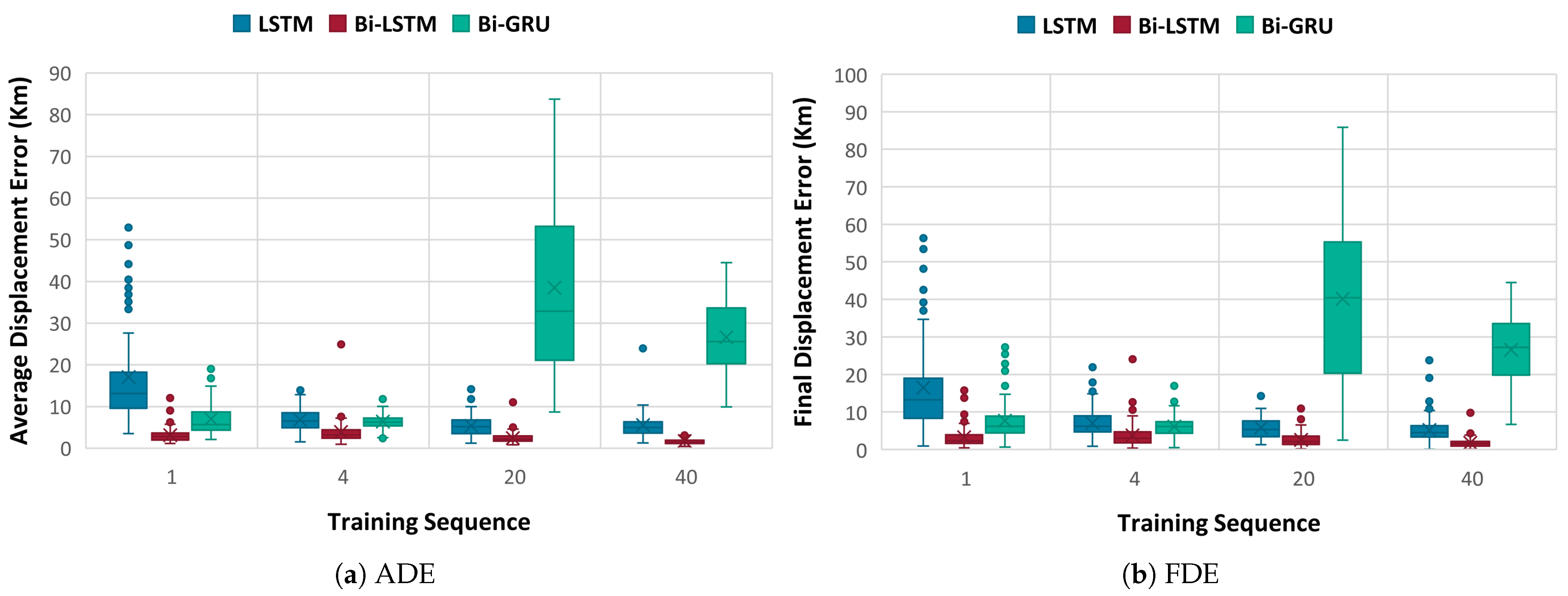
Figure 2 visualizes the ADE and FDE distributions using box and whisker plots for the short-term prediction of the three models across the four training sequences. Across all models and configurations, Bi-LSTM with longer sequence lengths demonstrated the most robust and accurate short-term forecasting. LSTM models performed well overall but experienced the most outliers, i.e., the trajectory predictions for some routes are very inaccurate with very high ADEs and FDEs. While LSTM models benefit from increased sequence length (up to a point), their capacity to capture bidirectional dependencies and mitigate error propagation remains limited in comparison to Bi-LSTM. In contrast, Bi-GRU models struggled to maintain performance at higher sequence lengths, raising concerns about their scalability and stability for short-term vessel trajectory forecasting. This performance divergence underscores the relative fragility of the Bi-GRU architecture in deep sequence modeling compared to the Bi-LSTM and LSTM counterparts. These findings underscore the critical role of architectural design and temporal depth in achieving reliable short-horizon predictions.

In addition to predictive accuracy, we evaluated the computational performance of the models to better understand their suitability for real-world deployment. Specifically, we measured training time (in minutes per epoch) and inference time (in milliseconds per prediction) across varying input sequence lengths, as shown in

Table 6. Training and inference times for models with different training sequence sizes.

Model	Training Sequence	Training Time (min/Epoch)	Inference Time (ms/Prediction)
LSTM	1	28.75	52.88
LSTM	4	38.91	52.96
LSTM	20	103.58	56.01
LSTM	40	193.53	59.43
Bi-LSTM	1	51.04	53.70
Bi-LSTM	4	75.15	54.49
Bi-LSTM	20	236.73	58.67
Bi-LSTM	40	418.18	62.83
Bi-GRU	1	46.14	53.60
Bi-GRU	4	63.22	54.16
Bi-GRU	20	180.15	58.38
Bi-GRU	40	296.40	62.01

. As expected, increasing the input training sequence from 1 to 40 data points led to a rise in training time for all models from approximately 30 min per epoch for LSTM to 400 min for Bi-LSTM. Inference time also increased but very modestly: from 52 ms to 62 ms per prediction for all models. While training time scales significantly with sequence length due to increased model complexity and temporal depth, the relatively low inference latency indicates that the models remain suitable for near-real-time trajectory prediction applications.

4.2. Long-Term Prediction Analysis Across Horizons

In trajectory forecasting tasks, the prediction horizon plays a critical role in determining model performance. While short-term prediction assumes access to ground-truth inputs at each time step, long-term prediction presents a more realistic and challenging scenario. In this setting, the model recursively uses its own previous outputs as inputs for future steps, potentially introducing cumulative error propagation.

In this section, we evaluate long-term prediction performance using the Bi-LSTM architecture trained on 40-point input sequences, since it exhibited the best predictive performance for single-point predictions. The evaluation is conducted across three prediction horizons: 20 points (10 min), 60 points (30 min), and 120 points (60 min). These configurations allow us to systematically assess how prediction accuracy behaves as the forecasting window increases, thereby providing insight into the model’s ability to maintain reliable performance over time.

Table 7. Long-term prediction metrics when using Bi-LSTM with a 40-point training sequence across multiple prediction horizons.

Prediction Sequence	20 Points (10 min)	60 Points (30 min)	120 Points (60 min)
ADE	5.3052	11.1432	18.6331
FDE	8.5026	19.0673	32.7800
DFD	8.7431	19.6947	33.5118
MAE
Latitude	0.0226	0.0462	0.0771
Longitude	0.0448	0.0953	0.1602
SoG	0.8982	1.7570	2.4021
CoG	12.6513	30.6923	46.0783
MSE
Latitude	0.0027	0.0062	0.0143
Longitude	0.0048	0.0187	0.0507
SoG	8.6617	22.5692	39.0892
CoG	644.5075	2406.9327	4742.5689
RMSE
Latitude	0.0517	0.0786	0.1197
Longitude	0.0695	0.1367	0.2252
SoG	2.9431	4.7507	6.2517
CoG	25.3866	49.0604	68.8845
SMAPE
Latitude	0.0675	0.1379	0.2302
Longitude	0.1499	0.3207	0.5389
SoG	24.1447	35.9006	44.4687
CoG	8.7546	21.3748	32.1960

shows the long-term prediction results across the multiple prediction horizons. As expected, even high-performing models such as Bi-LSTM experience performance degradation under long-term prediction scenarios as the horizon length increases. Predictions for the next 20 points (i.e., next 10 min) yield satisfactory results with ADE = 5.3 Km and FDE = 8.5. The DFD of 8.7 km suggests the worst-case trajectory deviation occurs early or stabilizes, leading the predicted path to remain within a rough spatial corridor, even if points are farther off on average. As the forecast horizon extends beyond the initial 40-point training sequence, errors accumulate due to the model’s recursive reliance on its own previous outputs, resulting in compounded inaccuracies. This deterioration is evident across displacement-based metrics as ADE and FDE increase to 18.6 Km and 32.8 Km, respectively, reflecting diminished spatial precision. Similarly, trajectory shape divergence, as measured by DFD, intensifies with longer horizons up to 33.5 Km. Further, point-based error metrics for key dynamic features (i.e., latitude, longitude, SoG, and CoG) exhibit pronounced growth, with angular variables such as CoG showing particularly steep error escalations.

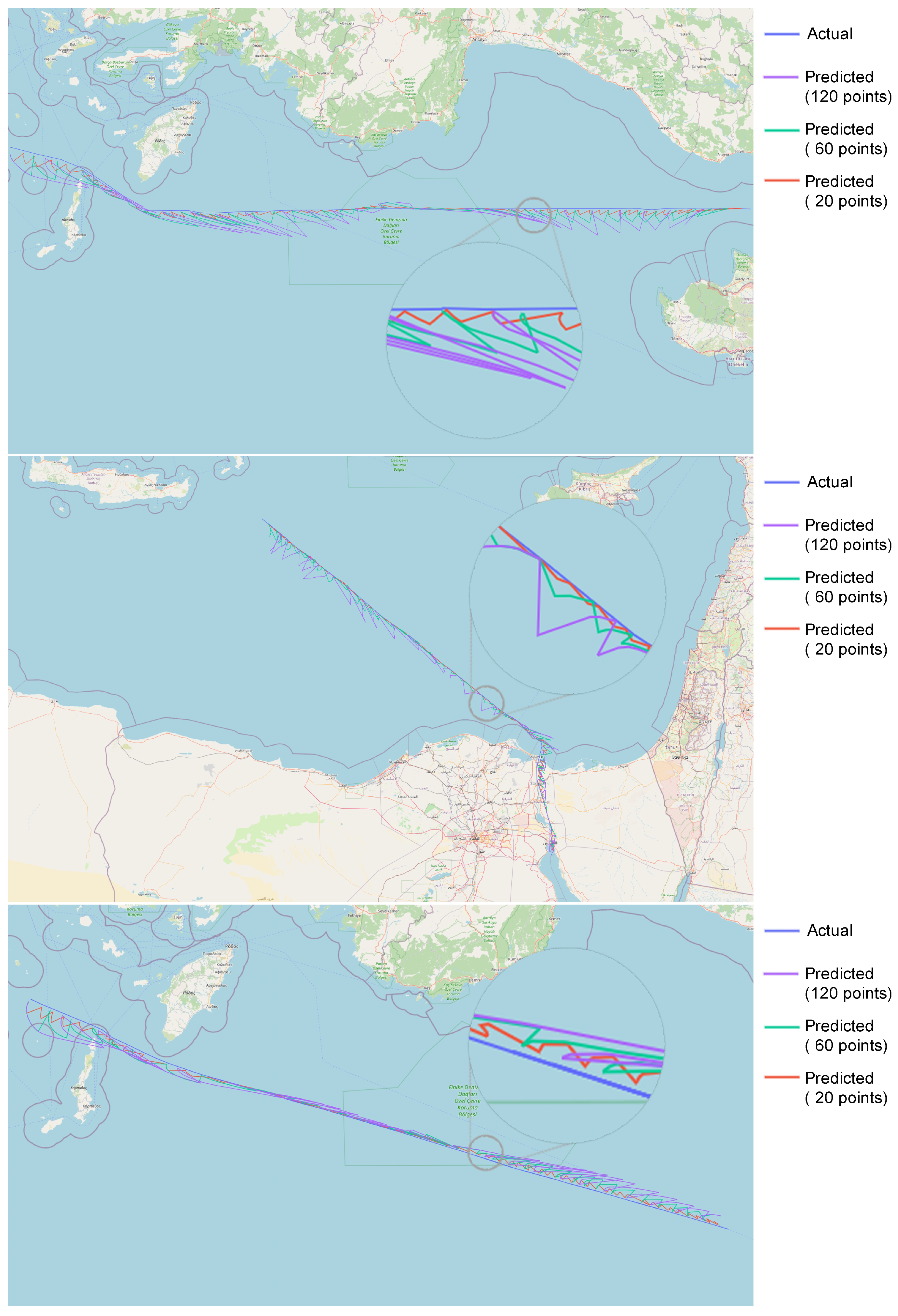
To qualitatively illustrate this behavior, Figure 3 presents visual comparisons between the ground-truth routes and Bi-LSTM predictions at 20-, 60-, and 120-point horizons for three representative vessel trajectories. The figures highlight the increasing divergence between predicted and actual paths as the forecast horizon lengthens, particularly in terms of directional drift and spatial displacement. The highest prediction errors in long-term vessel trajectory forecasting typically occur near regions where the vessel undergoes significant changes in direction. These directional transitions are often associated with navigational decisions, environmental responses (e.g., wind, current), or operational constraints, which introduce abrupt changes in movement patterns. Predictive models, especially those that rely heavily on short-term temporal dependencies, tend to struggle in capturing such nonlinear dynamics. As a result, prediction accuracy degrades in these regions, as evidenced by localized spikes in displacement error.

These findings underscore the inherent limitations of autoregressive sequence models in maintaining directional and spatial stability over extended predictions, highlighting the importance of evaluating models across both short- and long-term horizons to fully assess their practical viability in real-world applications. Moreover, they call attention to the necessity of developing strategies aimed at mitigating error propagation to enhance long-range forecasting reliability.

4.3. Long-Term Horizon to Threshold Analysis

In our final experiment, we evaluated the Bi-LSTM model’s long-term predictive performance in an open-loop setting, where the model generates the vessel’s future trajectory continuously from a single initial input sequence. Unlike segmented approaches, this setup does not introduce new observational inputs during inference; instead, the model relies entirely on its own recursive predictions to progress along the route. The initial input consists of a 40-point sequence, and the model proceeds without interruption for as many steps as required to reach the end of the actual route, enabling a realistic and unbounded assessment of long-term forecasting behavior.

To further assess the robustness of the Bi-LSTM model over extended prediction horizons, we conducted a time-to-threshold analysis, where we analyzed how quickly prediction errors surpass predefined spatial thresholds during recursive inference. Specifically, we measured the average number of minutes required for the prediction error to surpass a set of predefined spatial thresholds (5, 10, 20, 50, and 100 Km). The results, summarized in

Table 8. Time-to-threshold analysis results for long-term vessel trajectory predictions. The table reports the average number of minutes required for the prediction error to exceed each distance threshold, along with the number of routes (out of 100) where the threshold was eventually exceeded.

Distance Threshold (km)	Average Time to Threshold (min)	Number of Routes Exceeding the Threshold
5	10.60	98
10	20.78	96
20	43.72	92
50	112.58	82
100	296.51	75

, show that on average, it takes around 10 min for the error to exceed 5 km and 20 min to exceed 10 km, while exceeding 100 km takes nearly 297 min (around 5 h). In addition, we tracked the proportion of routes that ever crossed each threshold. We observed that almost all routes (98) exceeded the 5 km threshold eventually, whereas only 75 reached an error exceeding 100 km.

This trend illustrates the compounding nature of predictive error in long-term autoregressive forecasting. While most routes maintain a relatively low spatial error in the early stages of prediction, sustained accuracy becomes increasingly challenging to uphold over time. The decrease in the number of routes exceeding larger thresholds reflects either the natural capping of some route lengths or improved long-term performance on a subset of routes. This analysis provides a quantitative view of trajectory stability, helping identify thresholds of operational acceptability for different maritime applications. Finally, these findings reinforce the necessity of incorporating error mitigation strategies or hybrid correction mechanisms in real-world deployments where prolonged accuracy is critical.

5. Discussion

This study rigorously evaluates the predictive capabilities of three recurrent neural network architectures (i.e., LSTM, Bi-LSTM, and Bi-GRU) for vessel trajectory forecasting, with an emphasis on both short-term (single-step) and long-term (multi-step) prediction horizons. By systematically varying the input sequence length and employing both ground-truth-driven and autoregressive inference strategies, the analysis offers several key insights for the development of robust data-driven maritime trajectory forecasting models.

Among the tested architectures, the Bi-LSTM consistently delivered the highest overall performance. Notably, when trained with longer input sequences (e.g., 40 points), the Bi-LSTM demonstrated strong accuracy in predicting spatial (latitude, longitude) and dynamic (SoG, CoG) vessel attributes. Its ability to model bidirectional temporal dependencies allows it to extract richer contextual information from sequence data, leading to more coherent and temporally stable predictions. This finding corroborates previous studies underscoring the strength of bidirectional architectures in complex sequential tasks [12,14,34].

While the LSTM model achieved generally good results, it did not match the Bi-LSTM in terms of consistency or precision, particularly at longer input lengths. The Bi-GRU model exhibited highly unstable behavior when trained on extended sequences, with significant degradation in prediction quality. This may be attributed to its simpler gating mechanism, which, while faster to train, is potentially more vulnerable to gradient instability or overfitting in long-horizon contexts.

The shift to a multi-step long-term prediction framework, where vessel positions are predicted recursively for 10, 30, and 60 min into the future, provides a more realistic and operationally relevant assessment of model performance. The results indicate a clear pattern of error accumulation: while predictions at 10 min remain spatially close to the ground truth, performance deteriorates at 30 and 60 min, particularly in directional metrics such as CoG. This is a known limitation of autoregressive models, where small prediction errors compound over successive recursive inputs [15].

This trend is visualized in Figure 3, which depicts model predictions at all three horizons across representative vessel trajectories. The 10-min predictions align closely with actual routes, while the 30- and 60-min forecasts progressively diverge, though still maintaining the general route structure and directional intent. Such visualizations reinforce the model’s practical potential: despite increased uncertainty, Bi-LSTM preserves usable trajectory information over extended intervals without further AIS input.

Our final experiment assessed the Bi-LSTM model’s ability to predict long-term trajectory from a single 40-point input without additional observational updates. While the model demonstrated a strong short-term to mid-term accuracy, its performance declined steadily over time due to cumulative error propagation. Deviations became more pronounced beyond 30 min, particularly in directional and spatial metrics. Threshold-based analysis further revealed that although many routes remained accurate within short ranges, fewer sustained performance as the horizon extended. These results highlight the model’s effectiveness in short-range forecasting and its limitations over extended predictions, underscoring the need for strategies to mitigate long-term drift.

The time-to-threshold analysis in Section 4.3 provides critical insights into how prediction accuracy evolves over time and its potential alignment with real-world maritime operational requirements. In port approach scenarios [38], such as entering a port or navigating confined harbor channels, maintaining sub-5 km accuracy is essential for safe maneuvering, pilotage coordination, and berth planning. The result that a 5 km prediction error is typically not exceeded until approximately 10 min (in 98 out of 100 test routes) indicates that the model can reliably support near-term decisions such as assigning pilots or initiating tugboat dispatch with sufficient lead time.

For vessel traffic service (VTS) operations in controlled waterways, such as the Bosporus Strait or Dover TSS, accurate medium-term predictions with errors below 10–20 km are crucial for maintaining safe separation between vessels and preventing conflicts [39]. The model’s ability to remain within a 10 km error margin for roughly 21 min and within 20 km for over 43 min suggests practical utility for VTS centers’ monitoring vessel flows and issuing advisories. This could also support early conflict detection in dense traffic scenarios under COLREGS (the International Regulations for Preventing Collisions at Sea) Rule 7 (Risk of Collision) [40].

At the strategic level, the longer thresholds (50 km exceeded after 112 min and 100 km after nearly 5 h) are more relevant for autonomous navigation systems and voyage optimization platforms [41]. These applications require coarse long-range situational awareness for path planning, fuel consumption forecasting, or dynamic ETA estimation. The delayed breach of larger thresholds suggests the model can contribute meaningfully to route-level decisions, even without frequent retraining or reinitialization.

These findings underscore both the promise and limitations of current recurrent approaches in long-range trajectory forecasting. To address these challenges, future work should focus on improving the model’s sensitivity to context-dependent maneuvers, potentially by integrating auxiliary inputs such as heading change rates, sea state conditions, or proximity to navigational turning points. Additionally, hybrid models that blend data-driven learning with rule-based maneuver detection may offer better robustness in handling abrupt course changes.

While this study focuses on the eastern Mediterranean region, the dataset encompasses a wide range of vessel types and operational scenarios, supporting the broader applicability of the findings. This diversity enhances the robustness of the evaluation and suggests that the insights gained from this study are relevant to a broad set of maritime forecasting scenarios. Nonetheless, future work could extend this analysis to other geographic regions and incorporate additional contextual factors such as weather, traffic density, and regulatory constraints to further assess model generalizability.

To further extend long-term predictions, future work should explore model architectures explicitly designed to mitigate recursive error propagation. Approaches such as scheduled sampling, noise-aware training, or sequence-level loss functions could improve predictive stability over extended horizons and further enhance the practical applicability of deep learning-based trajectory forecasting systems. In addition, attention-based architectures like the Transformer [42] show promise in this domain. Unlike recurrent models, Transformers can attend selectively to relevant temporal contexts without relying on iterative state updates, offering a pathway to more stable and accurate long-term predictions.

6. Conclusions

This work contributes to the understanding of recurrent architectures for vessel trajectory prediction by providing empirical evidence and practical insights for model design and deployment. Bi-LSTM models outperform LSTM and Bi-GRU, particularly with longer input sequences, highlighting the strength of bidirectional architectures in capturing complex spatiotemporal dependencies. While longer input sequences improve predictive accuracy, they also increase model complexity and training challenges, especially for Bi-GRU, underscoring the importance of careful model selection and tuning. Our findings also show that short-term prediction evaluations can overestimate real-world performance, while long-term recursive forecasting can lead to error accumulation and reduced accuracy over time. Despite these challenges, Bi-LSTM maintains reasonable trajectory coherence over extended horizons, supporting its applicability for operational maritime applications within defined spatial and temporal bounds. Future research should explore architectures like Transformers and training strategies that mitigate recursive errors to enhance long-term forecasting capabilities.